跳到论文正文
W Papers独立论文阅读器 arXiv:1801.09884 论文正文 计算阅读时间 · 0%
引用这篇论文根据当前论文元数据生成,正式投稿前建议核对。


License: arXiv.org perpetual non-exclusive license
arXiv:1801.09884v2 [math.ST] 25 Jul 2018

Estimation of conditional extreme risk measures from heavy-tailed elliptical random vectors

A. Usseglio-Carleve Address: Université de Lyon, Université Lyon 1, Institut Camille Jordan ICJ UMR 5208 CNRS Email address: usseglio@math.univ-lyon1.fr
Abstract.

In this work, we focus on some conditional extreme risk measures estimation for elliptical random vectors. In a previous paper, we proposed a methodology to approximate extreme quantiles, based on two extremal parameters. We thus propose some estimators for these parameters, and study their consistency and asymptotic normality in the case of heavy-tailed distributions. Thereafter, from these parameters, we construct extreme conditional quantiles estimators, and give some conditions that ensure consistency and asymptotic normality. Using recent results on the asymptotic relationship between quantiles and other risk measures, we deduce estimators for extreme conditional Lp−L_{p}-quantiles and Haezendonck-Goovaerts risk measures. Under similar conditions, consistency and asymptotic normality are provided. In order to test the effectiveness of our estimators, we propose a simulation study. A financial data example is also proposed.

Key words and phrases:
Elliptical distribution; Extreme quantiles; Extreme value theory; Haezendonck-Goovaerts risk measures; Heavy-tailed distributions; Lp−L_{p}-quantiles.

Keywords:

1. Introduction

In many fields such as finance or actuarial science, quantile, or Value-at-Risk (see Linsmeier and Pearson, (2000)) is a recognized tool for risk measurement. In Koenker and Bassett, (1978), quantile is seen as minimum of an asymmetric loss function. However, Value-at-Risk, or VaR, has some disadvantages, such as that of not being a coherent measure in the sense of Artzner et al., (1999). These limits have led many authors to use alternative risk measures.
On the basis of Koenker’s approach, Newey and Powell, (1987) proposed another measure called expectile, which has since been widely studied (see for example Sobotka and Kneib, (2012) or more recently Daouia et al., 2017a ()) and applied (Taylor, (2008) and Cai and Weng, (2016)). Later, Breckling and Chambers, (1988) introduced M-quantiles, a family of measures minimizing an asymmetric loss function, and Chen, (1996) focused on asymmetric power functions to define Lp−L_{p}-quantiles. The cases p=1p=1 and p=2p=2 correspond respectively to the quantile and expectile. Recently, Bernardi et al., (2017) provided some results concerning Lp−L_{p}-quantiles for Student distributions, and have shown that closed formula are difficult to obtain in the general case.
In parallel, Artzner et al., (1999) introduced the Tail-Value-at-Risk as an alternative to Value-at-Risk, and this risk measure subsequently had many applications (see e.g. Bargès et al., (2009)). Moreover, TVaR belongs to a larger family of risk measures called Haezendonck-Goovaerts risk measures and introduced in Haezendonck and Goovaerts, (1982), Goovaerts et al., (2004) and Tang and Yang, (2012). In the same way as Lp−L_{p}-quantiles, we do not have an explicit formula in the general case.
However, for a heavy-tailed random variable, Daouia et al., 2017b () proved that Lp−L_{p}-quantile and L1−L_{1}-quantile (or quantile) are asymptotically proportional. Then, as proposed in Daouia et al., 2017a (), an estimator of a Lp−L_{p}-quantile may be deduced from a suitable estimator of the quantile, for extreme levels. In the same spirit, Tang and Yang, (2012) provided a similar asymptotic relationship between a subclass of Haezendonck-Goovaerts risk measures and quantiles. Finally, all these risk measures we introduced may be estimated through a quantile estimation in an asymptotic setting.
Extreme quantiles estimation is a very active area of research. In recent years, we can give many examples : Gardes and Girard, (2005) focused on Weibull tail distributions, El Methni et al., (2012) proposed a study for heavy and light tailed distributions, Gong et al., (2015) was interested in functions of dependent variables, and de Valk, (2016) provided a methodology for high quantiles estimation. The question of extreme conditional quantiles estimation has also been explored in Wang et al., (2012) in a regression framework. However, Maume-Deschamps et al., (2017) and Maume-Deschamps et al., (2018) have shown that the regression setting may lead to a poor estimation of extreme measures in the case of elliptical distributions. Elliptical distributions, introduced in Kelker, (1970), aim to generalize the gaussian distribution, i.e to define symmetric distributions with different properties, such as a heavy tail. This is why elliptical distributions are more and more used in finance (see for example Owen and Rabinovitch, (1983) or Xiao and Valdez, (2015)).
For all these reasons, we consider, in this paper, an elliptical random vector 𝒁=(𝑿,Y){\boldsymbol{Z}}=({\boldsymbol{X}},Y) with the consistency property (in the sense of Kano, (1994)), where 𝑿∈ℝN{\boldsymbol{X}}\in\mathbb{R}^{N}, Y∈ℝY\in\mathbb{R}, and propose to estimate some extreme quantiles (and deduce Lp−L_{p}-quantiles and Haezendonck-Goovaerts risk measures) of Y|𝑿=𝒙Y|{\boldsymbol{X}}={\boldsymbol{x}}, i.e. of a component conditionnally to the others. In order to improve the conditional quantile estimation, we proposed in Maume-Deschamps et al., (2017) a methodology based on two extremal parameters, and the unconditional quantile of YY. Indeed, if we denote FY|𝒙−1​(α)F_{Y|{\boldsymbol{x}}}^{-1}(\alpha) the quantile of level α\alpha of Y|𝑿=𝒙Y|{\boldsymbol{X}}={\boldsymbol{x}}, the latter is asymptotically equivalent to a quantile of YY (FY−1F_{Y}^{-1} will be the quantile function of YY), in the following manner :

(1.1) FY|𝒙−1​(α)​∼α→1​FY−1​(δ⁡(α,η,ℓ)),F_{Y|{\boldsymbol{x}}}^{-1}(\alpha)\underset{\alpha\rightarrow 1}{\sim}F_{Y}^{-1}\left(\delta(\alpha,\eta,\ell)\right),

where δ\delta is a known function (detailed later) depending on α\alpha and two parameters η\eta and ℓ\ell called extremal parameters. One can notice that Equation (1.1) may only holds under the consistency property of 𝒁{\boldsymbol{Z}}. Maume-Deschamps et al., (2017) has also shown that extremal parameters do not exist for some consistent elliptical distributions (see e.g. the Laplace distribution).
In this paper, the goal will be in a first time to give a sufficient condition on 𝒁{\boldsymbol{Z}} that ensures the existence of η\eta and ℓ\ell. This is why a regularly varying assumption is done. After having proved their existence, estimators for the parameters η\eta and ℓ\ell are proposed, and therefore for extreme conditional quantiles.
The paper is organized as follows. Section 2 provides some definitions and properties of elliptical distributions, including the extremal parameters introduced in Maume-Deschamps et al., (2017). A particular interest is given to consistent elliptical distributions. Section 3 is devoted to extremal parameters η\eta and ℓ\ell. Under a regularly varying assumption, their existence is proved, and estimators are proposed. By adding some conditions, consistency and asymptotic normality results are given. In Section 4, we use the results of Section 3 to introduce some estimators of extreme quantiles, and give consistency and asymptotic normality results. The asymptotic relationships between Lp−L_{p}-quantiles and quantiles recalled in Section 5 allow us to give extreme Lp−L_{p}-quantiles estimators. The same approach is proposed for extreme Haezendonck-Goovaerts risk measures. In order to analyze the efficiency of our estimators, we propose a simulation study in Section 6, and a real data example in Section 7.

2. Preliminaries

In this section, we first recall some classical results on elliptical distributions. We consider a d−d-dimensional vector 𝒁{\boldsymbol{Z}} from an elliptical distribution with parameters 𝝁∈ℝd{\boldsymbol{\mu}}\in\mathbb{R}^{d} and 𝚺∈ℝd×d{\boldsymbol{\Sigma}}\in\mathbb{R}^{d\times d}. Then the density of 𝒁{\boldsymbol{Z}}, if it exists, is given by :

(2.1) cd|𝚺|12​gd​((𝒛−𝝁)T​𝚺−1​(𝒛−𝝁)).\frac{c_{d}}{|{\boldsymbol{\Sigma}}|^{\frac{1}{2}}}g_{d}\left(\left({\boldsymbol{z}}-{\boldsymbol{\mu}}\right)^{T}{\boldsymbol{\Sigma}}^{-1}\left({\boldsymbol{z}}-{\boldsymbol{\mu}}\right)\right).

cdc_{d} and gdg_{d} will respectively be called normalization coefficient and generator of 𝒁{\boldsymbol{Z}}. Cambanis et al., (1981) gives another way to characterize an elliptical distribution, through the following stochastic representation :

(2.2) 𝒁​=𝑑​𝝁+R​𝚲​𝑼(d),{\boldsymbol{Z}}\overset{d}{=}{\boldsymbol{\mu}}+R{\boldsymbol{\Lambda}}{\boldsymbol{U}}^{(d)},

where 𝚲​𝚲T=𝚺{\boldsymbol{\Lambda}}{\boldsymbol{\Lambda}}^{T}={\boldsymbol{\Sigma}}, 𝑼(d){\boldsymbol{U}}^{(d)} is a d−d-dimensional random vector uniformly distributed on the unit sphere of dimension dd, and RR is a non-negative random variable independent of 𝑼(d){\boldsymbol{U}}^{(d)}. RR is called radius of 𝒁{\boldsymbol{Z}}. In the following, the radius must have a particular shape. Indeed, Huang and Cambanis, (1979) and Kano, (1994) propose a representation for some particular elliptical distributions. Let us consider (𝒁d)d∈ℕ∗\left({\boldsymbol{Z}}_{d}\right)_{d\in\mathbb{N}^{*}} a family of elliptical distributions of dimension dd. Then (𝒁d)d∈ℕ∗\left({\boldsymbol{Z}}_{d}\right)_{d\in\mathbb{N}^{*}} possesses the consistency property if it admits the following representation for all d∈ℕ∗d\in\mathbb{N}^{*} :

(2.3) 𝒁d​=𝑑​𝝁+χd​ξ​𝚲​𝑼(d),{\boldsymbol{Z}}_{d}\overset{d}{=}{\boldsymbol{\mu}}+\chi_{d}\xi{\boldsymbol{\Lambda}}{\boldsymbol{U}}^{(d)},

where χd\chi_{d} is the square root of a χ2\chi^{2} distribution with dd degrees of freedom, ξ\xi is a non-negative random variable which does not depend on dd, and χd\chi_{d}, ξ\xi and 𝑼(d){\boldsymbol{U}}^{(d)} are mutually independent. In Kano, (1994), such elliptical distributions are said consistent, have the advantage of being stable by linear combinations (combining Theorem 2.16 of Fang et al., (1990) and Theorem 1 in Kano, (1994)), and allow us to define elliptical random fields (see, e.g., Opitz, (2016)). In the following, we focus on consistent elliptical distributions, and take the notation

(2.4) Rd=χd​ξ.R_{d}=\chi_{d}\xi.

For the sake of clarity, we will say that a random variable with stochastic representation (2.3) is (ξ,d)−(\xi,d)-elliptical with parameters 𝝁{\boldsymbol{\mu}} and 𝚺{\boldsymbol{\Sigma}}. Using this terminology, the purpose of the paper is as follows. Let 𝒁=(𝑿,Y)∈ℝN+1{\boldsymbol{Z}}=({\boldsymbol{X}},Y)\in\mathbb{R}^{N+1} be a (ξ,N+1)−(\xi,N+1)-elliptical random vector with parameters 𝝁{\boldsymbol{\mu}} and 𝚺{\boldsymbol{\Sigma}}, where 𝑿∈ℝN{\boldsymbol{X}}\in\mathbb{R}^{N} and Y∈ℝY\in\mathbb{R}. Consistency property of 𝒁{\boldsymbol{Z}} implies that 𝑿{\boldsymbol{X}} and YY are respectively (ξ,N)−(\xi,N)- and (ξ,1)−(\xi,1)-elliptical distributions with parameters 𝝁𝑿∈ℝN{\boldsymbol{\mu_{X}}}\in\mathbb{R}^{N}, 𝚺𝑿∈ℝN×N{\boldsymbol{\Sigma_{X}}}\in\mathbb{R}^{N\times N} and μY∈ℝ\mu_{Y}\in\mathbb{R}, ΣY∈ℝ\Sigma_{Y}\in\mathbb{R}. We also denote 𝚺𝑿​Y{\boldsymbol{\Sigma}}_{{\boldsymbol{X}}Y} the covariance vector between 𝑿{\boldsymbol{X}} and YY. The aim is thus to provide a predictor for the quantile of the conditional distribution Y|𝑿=𝒙Y|{\boldsymbol{X}}={\boldsymbol{x}}. According to Theorem 7 of Frahm, (2004), such a distribution is still elliptical, with a radius R∗R^{*} different from RR in the general case. In particular, we have :

(2.5) {Y|𝑿=𝒙}​=𝑑​μY|𝑿+σY|𝑿​R∗​U(1),\{Y|{\boldsymbol{X}}={\boldsymbol{x}}\}\overset{d}{=}\mu_{Y|{\boldsymbol{X}}}+\sigma_{Y|{\boldsymbol{X}}}R^{*}U^{(1)},

where μY|𝑿=μY+𝚺𝑿​YT​𝚺𝑿−1​(𝒙−𝝁𝑿)\mu_{Y|{\boldsymbol{X}}}=\mu_{Y}+{\boldsymbol{\Sigma}}_{{\boldsymbol{X}}Y}^{T}{\boldsymbol{\Sigma_{X}}}^{-1}({\boldsymbol{x}}-{\boldsymbol{\mu_{X}}}) and σY|𝑿2=ΣY−𝚺𝑿​YT​𝚺𝑿−1​𝚺𝑿​Y\sigma_{Y|{\boldsymbol{X}}}^{2}=\Sigma_{Y}-{\boldsymbol{\Sigma}}_{{\boldsymbol{X}}Y}^{T}{\boldsymbol{\Sigma_{X}}}^{-1}{\boldsymbol{\Sigma}}_{{\boldsymbol{X}}Y}. Then, denoting ΦR∗​(t)=ℙ⁡(R∗​U(1)≤t)\Phi_{R^{*}}(t)=\mathbb{P}\left(R^{*}U^{(1)}\leq t\right), and using the translation equivariance and positive homogeneity of elliptical quantiles (see McNeil et al., (2015)), conditional quantiles of Y|𝑿=𝒙Y|{\boldsymbol{X}}={\boldsymbol{x}} may be expressed as :

(2.6) qα​(Y|𝑿=𝒙)=μY|𝑿+σY|𝑿​ΦR∗−1​(α),q_{\alpha}(Y|{\boldsymbol{X}}={\boldsymbol{x}})=\mu_{Y|{\boldsymbol{X}}}+\sigma_{Y|{\boldsymbol{X}}}\Phi_{R^{*}}^{-1}(\alpha),

where α∈]0,1[\alpha\in]0,1[. Thus, in order to give a good prediction of qα​(Y|𝑿=𝒙)q_{\alpha}(Y|{\boldsymbol{X}}={\boldsymbol{x}}), we need to estimate the conditional function ΦR∗−1\Phi_{R^{*}}^{-1}. Unfortunately, when we have a data set 𝑿1,…,𝑿n{\boldsymbol{X}}_{1},...,{\boldsymbol{X}}_{n}, we only observe the unconditional distribution of 𝑿{\boldsymbol{X}}. This is why, in Maume-Deschamps et al., (2017), we have given a predictor for conditional quantiles, based solely on the unconditional c.d.f ΦR​(t)=ℙ⁡(R1​U(1)≤t)\Phi_{R}(t)=\mathbb{P}\left(R_{1}U^{(1)}\leq t\right). This approximation is based on two parameters η∈ℝ\eta\in\mathbb{R} and 0<ℓ<+∞0<\ell<+\infty such that :

(2.7) limt→∞ Φ¯R∗​(t)Φ¯R​(tη)=ℓ.\underset{t\rightarrow\infty}{\lim}\text{ }\frac{\bar{\Phi}_{R^{*}}(t)}{\bar{\Phi}_{R}(t^{\eta})}=\ell.

Table 1 gives some examples of coefficients η\eta and ℓ\ell for classical elliptical distributions.

Distribution η\eta ℓ\ell
Gaussian 11 11
Student, ν>0\nu>0 Nν+1\frac{N}{\nu}+1 Γ⁡(ν+N+12)​Γ​(ν2)Γ⁡(ν+N2)​Γ​(ν+12)​(1+M⁡(𝒙)ν)N+ν2​νN2+1ν+N\frac{\Gamma\left(\frac{\nu+N+1}{2}\right)\Gamma\left(\frac{\nu}{2}\right)}{\Gamma\left(\frac{\nu+N}{2}\right)\Gamma\left(\frac{\nu+1}{2}\right)}\left(1+\frac{M({\boldsymbol{x}})}{\nu}\right)^{\frac{N+\nu}{2}}\frac{\nu^{\frac{N}{2}+1}}{\nu+N}
UGM 11 min⁡(θ1,…,θn)N​exp​{−min⁡(θ1,…,θn)22​M​(𝐱)}∑k=1nπk​θkN​exp⁡(−θk22​M​(𝒙))\frac{\rm\min(\theta_{1},\ldots,\theta_{n})^{N}\exp\left\{-\frac{\rm\min(\theta_{1},\ldots,\theta_{n})^{2}}{2}M({\boldsymbol{x}})\right\}}{\sum\limits_{k=1}^{n}\pi_{k}\theta_{k}^{N}\exp\left(-\frac{\theta_{k}^{2}}{2}M({\boldsymbol{x}})\right)}
Slash, a>0a>0 Na+1\frac{N}{a}+1 Γ⁡(N+1+a2)​M​(𝒙)N+a2Γ⁡(N+a2)​(N+a)​χN+a2​(M⁡(𝒙))​2a2−1​Γ​(1+a2)\frac{\Gamma\left(\frac{N+1+a}{2}\right)M({\boldsymbol{x}})^{\frac{N+a}{2}}}{\Gamma\left(\frac{N+a}{2}\right)(N+a)\chi_{N+a}^{2}\left(M({\boldsymbol{x}})\right)2^{\frac{a}{2}-1}\Gamma\left(\frac{1+a}{2}\right)}
Table 1. Coefficients η\eta and ℓ\ell for classical distributions, where M⁡(𝒙)=(𝒙−𝝁𝑿)⊤​𝚺𝑿−1​(𝒙−𝝁𝑿)M({\boldsymbol{x}})=({\boldsymbol{x}}-{\boldsymbol{\mu_{X}}})^{\top}{\boldsymbol{\Sigma_{X}}}^{-1}({\boldsymbol{x}}-{\boldsymbol{\mu_{X}}}).

However, we have shown in Maume-Deschamps et al., (2017) that such parameters not always exist for all elliptical distribution (see, e.g, Laplace distribution). In a first time, we can wonder in which setting these parameters exist. We thus consider the following assumption, that will ensures the existence of η\eta and ℓ\ell.

Assumption 1 (Second order regular variations).

We assume that there exist a function AA such that A⁡(t)→0A(t)\rightarrow 0 as t→+∞t\rightarrow+\infty, and

(2.8) limt→+∞​ΦR−1​(1−1ω​t)ΦR−1​(1−1t)−ωγA⁡(t)=ωγ​ωρ−1ρ,\underset{t\rightarrow+\infty}{\lim}\frac{\frac{\Phi_{R}^{-1}\left(1-\frac{1}{\omega t}\right)}{\Phi_{R}^{-1}\left(1-\frac{1}{t}\right)}-\omega^{\gamma}}{A(t)}=\omega^{\gamma}\frac{\omega^{\rho}-1}{\rho},

where γ>0\gamma>0 and ρ<0\rho<0.

This assumption is widespread in literature of extreme quantiles (see, e.g, Daouia et al., 2017a ()). A first consequence is that ΦR\Phi_{R}, or equivalently FR1F_{R_{1}} is attracted to the maximum domain of Pareto-type distributions with tail index γ\gamma. Furthermore, it entails ΦR−1​(1−1/t)∼c1​tγ\Phi_{R}^{-1}(1-1/t)\sim c_{1}t^{\gamma}, or equivalently Φ¯R​(t)∼c2​t−1γ\bar{\Phi}_{R}(t)\sim c_{2}t^{-\frac{1}{\gamma}} as t→+∞t\rightarrow+\infty (see de Haan and Ferreira, (2006)). As example, Student distribution satisfies Assumption 1. The following lemma provides some results concerning asymptotic equivalences.

Lemma 2.1 (Regular variation properties).

Under Assumption 1, we get the following regular variations properties :

  1. (i)

    The random variable ξ\xi satisfies

    (2.9) F¯ξ​(t)​∼t→+∞​λ​t−1γ,λ∈ℝ.\bar{F}_{\xi}(t)\underset{t\rightarrow+\infty}{\sim}\lambda t^{-\frac{1}{\gamma}},\lambda\in\mathbb{R}.
  2. (ii)

    For all d∈ℕ∗d\in\mathbb{N}^{*}, the random variable Rd=χd​ξR_{d}=\chi_{d}\xi is attracted to the maximum domain of Pareto-type distribution with tail index γ\gamma, and

    (2.10) F¯Rd​(t)​∼t→+∞​212​γ​Γ⁡(d+γ−12)Γ⁡(d2)​F¯ξ​(t)​∼t→+∞​212​γ​Γ⁡(d+γ−12)Γ⁡(d2)​λ​t−1γ,λ∈ℝ.\bar{F}_{R_{d}}(t)\underset{t\rightarrow+\infty}{\sim}2^{\frac{1}{2\gamma}}\frac{\Gamma\left(\frac{d+\gamma^{-1}}{2}\right)}{\Gamma\left(\frac{d}{2}\right)}\bar{F}_{\xi}(t)\underset{t\rightarrow+\infty}{\sim}2^{\frac{1}{2\gamma}}\frac{\Gamma\left(\frac{d+\gamma^{-1}}{2}\right)}{\Gamma\left(\frac{d}{2}\right)}\lambda t^{-\frac{1}{\gamma}},\lambda\in\mathbb{R}.
  3. (iii)

    For all η>0\eta>0, d∈ℕ∗d\in\mathbb{N}^{*},

    (2.11) fRd​(t)fR1​(tη)​∼t→+∞​π​Γ​(d+γ−12)Γ⁡(d2)​Γ​(1+γ−12)​t(η−1)​(γ−1+1).\frac{f_{R_{d}}(t)}{f_{R_{1}}(t^{\eta})}\underset{t\rightarrow+\infty}{\sim}\frac{\sqrt{\pi}\Gamma\left(\frac{d+\gamma^{-1}}{2}\right)}{\Gamma\left(\frac{d}{2}\right)\Gamma\left(\frac{1+\gamma^{-1}}{2}\right)}t^{(\eta-1)(\gamma^{-1}+1)}.

These results will be usefull throughout the paper, and especially in the following result which proves the existence of our parameters.

Proposition 2.2 (Existence of extremal parameters).

Under Assumption 1, parameters η\eta and ℓ\ell exist, and are expressed :

(2.12) {η=1+γ​Nℓ=Γ⁡(N+γ−1+12)Γ⁡(γ−1+12)​γ−1​π−N2(N+γ−1)​cN​gN​(M⁡(𝒙)).\left\{\begin{array}[]{cc}\eta=&1+\gamma N\\ \ell=&\frac{\Gamma\left(\frac{N+\gamma^{-1}+1}{2}\right)}{\Gamma\left(\frac{\gamma^{-1}+1}{2}\right)}\frac{\gamma^{-1}\pi^{-\frac{N}{2}}}{(N+\gamma^{-1})c_{N}g_{N}\left(M({\boldsymbol{x}})\right)}\\ \end{array}\right..

One can notice that η\eta is only related to the tail index γ\gamma, and not to the covariate vector 𝒙{\boldsymbol{x}}, while ℓ\ell is depending on cN​gN​(M⁡(𝒙))c_{N}g_{N}\left(M({\boldsymbol{x}})\right). In the next, we thus denote rather ℓ⁡(𝒙)\ell({\boldsymbol{x}}), in order to emphasize the role played by the covariate vector 𝒙{\boldsymbol{x}}. We can now give the following predictor for qα​(Y|𝑿=𝒙)q_{\alpha}\left(Y|{\boldsymbol{X}}={\boldsymbol{x}}\right) :

(2.13) qα↑​(Y|𝑿=𝒙)=μY|𝑿+σY|𝑿​[ΦR−1​{1−1ℓ⁡(𝒙)1−α+2​(1−ℓ​(𝒙))}]1/η.q_{\alpha\uparrow}(Y|{\boldsymbol{X}}={\boldsymbol{x}})=\mu_{Y|{\boldsymbol{X}}}+\sigma_{Y|{\boldsymbol{X}}}\left[\Phi_{R}^{-1}\left\{1-\frac{1}{\frac{\ell({\boldsymbol{x}})}{1-\alpha}+2(1-\ell({\boldsymbol{x}}))}\right\}\right]^{{1}/{\eta}}.

From there, we have proved in Theorem 7 of Maume-Deschamps et al., (2017) that qα↑​(Y|𝑿=𝒙)q_{\alpha\uparrow}(Y|{\boldsymbol{X}}={\boldsymbol{x}}) and qα​(Y|𝑿=𝒙)q_{\alpha}(Y|{\boldsymbol{X}}={\boldsymbol{x}}) were asymptoticaly equivalent as α→1\alpha\rightarrow 1, i.e

(2.14) qα↑​(Y|𝑿=𝒙)​∼α→1​qα​(Y|𝑿=𝒙).q_{\alpha\uparrow}(Y|{\boldsymbol{X}}={\boldsymbol{x}})\underset{\alpha\rightarrow 1}{\sim}q_{\alpha}(Y|{\boldsymbol{X}}={\boldsymbol{x}}).

A similar equivalence has been easily deduced for α→0\alpha\rightarrow 0, using the symmetry properties of elliptical distributions. In this paper, we focus on the case α→1\alpha\rightarrow 1, case α→0\alpha\rightarrow 0 being easily deduced. In Section 3, we propose some estimators for extremal parameters η\eta and ℓ⁡(𝒙)\ell({\boldsymbol{x}}). Before that, we need to do a little simplification. Indeed, Equation (2.13) shows that the extreme quantile estimation requires the prior estimation of quantities μY|𝑿\mu_{Y|{\boldsymbol{X}}} and σY|𝑿\sigma_{Y|{\boldsymbol{X}}}. These quantities may be easily estimated by the method of moments or fixed-point algorithm (c.f p.66 of Frahm, (2004)). In a spatial setting, even if the variable YY is not observed, a stationarity assumption on the random field makes it possible to estimate these values (see Cressie, (1988)). Furthermore, the speed of convergence of these methods is higher than those of the estimators we propose in this paper, and therefore do not interfere in the asymptotic results. This is why, in the following, we suppose that μY|𝑿\mu_{Y|{\boldsymbol{X}}}, σY|𝑿\sigma_{Y|{\boldsymbol{X}}}, and therefore 𝝁𝑿{\boldsymbol{\mu_{X}}}, 𝚺𝑿{\boldsymbol{\Sigma_{X}}} are known. Then, it remains to estimate η\eta, ℓ⁡(𝒙)\ell({\boldsymbol{x}}) and ΦR∗−1\Phi_{R^{*}}^{-1}. Section 3 focuses on η\eta and ℓ⁡(𝒙)\ell({\boldsymbol{x}}), while Section 4 deals with ΦR∗−1\Phi_{R^{*}}^{-1}.

3. Extremal coefficients estimation

In this section, the aim is to estimate the extremal parameters η\eta and ℓ⁡(𝒙)\ell({\boldsymbol{x}}) conditionaly to the covariates vector 𝑿=𝒙{\boldsymbol{X}}={\boldsymbol{x}}. For that purpose, we consider a random sample 𝑿1,…,𝑿n{\boldsymbol{X}}_{1},...,{\boldsymbol{X}}_{n} independent and identically distributed from an (ξ,N)−(\xi,N)-elliptical vector with the same distribution as 𝑿{\boldsymbol{X}}, and denote M⁡(𝒙)=(𝒙−𝝁𝑿)T​𝚺𝑿−1​(𝒙−𝝁𝑿)M({\boldsymbol{x}})=\left({\boldsymbol{x}}-{\boldsymbol{\mu_{X}}}\right)^{T}{\boldsymbol{\Sigma_{X}}}^{-1}\left({\boldsymbol{x}}-{\boldsymbol{\mu_{X}}}\right). The aim is then to give two suitable estimator η^\hat{\eta} and ℓ^​(𝒙)\hat{\ell}({\boldsymbol{x}}), respectively for η\eta and ℓ⁡(𝒙)\ell({\boldsymbol{x}}).

3.1. Estimation of η\eta

We notice that coefficient η\eta is directly related on the tail index γ\gamma. Then, using a suitable estimator of γ\gamma, we easily deduce η\eta. There are several estimators widespread in the literature. As examples, Pickands, (1975), Schultze and Steinebach, (1996) or Kratz and Resnick, (1996) provide some estimators for γ\gamma. In the following, we use the Hill estimator, introduced in Hill, (1975) :

(3.1) γ^kn=1kn​∑i=1knln⁡(W[i]W[kn+1]),\hat{\gamma}_{k_{n}}=\frac{1}{k_{n}}\sum\limits_{i=1}^{k_{n}}\ln\left(\frac{W_{[i]}}{W_{[k_{n}+1]}}\right),

where W[1]≥…≥W[kn+1]≥…≥W[n]W_{[1]}\geq\ldots\geq W_{[k_{n}+1]}\geq\ldots\geq W_{[n]} and kn=o⁡(n)k_{n}=o(n) such that kn→+∞k_{n}\rightarrow+\infty as n→+∞n\rightarrow+\infty. In this context, the statistic WW may be :

  • •

    The first (or indifferently any) component of the reduced centered covariate vector 𝚲𝑿−1​(𝑿−𝝁𝑿){\boldsymbol{\Lambda_{X}}}^{-1}\left({\boldsymbol{X}}-{\boldsymbol{\mu_{X}}}\right), where 𝚲𝑿T​𝚲𝑿=𝚺𝑿{\boldsymbol{\Lambda_{X}}}^{T}{\boldsymbol{\Lambda_{X}}}={\boldsymbol{\Sigma_{X}}}. This approach works well, but we do not use all available data.

  • •

    The Mahalanobis norm (𝑿−𝝁𝑿)T​𝚺𝑿−1​(𝑿−𝝁𝑿)\sqrt{({\boldsymbol{X}}-{\boldsymbol{\mu_{X}}})^{T}{\boldsymbol{\Sigma_{X}}}^{-1}({\boldsymbol{X}}-{\boldsymbol{\mu_{X}}})}. This approach has the advantage of using all available data.

Indeed, according to Theorem 2 of Hashorva, 2007b (), the two last quantities both admit γ\gamma as tail index.
In the following we will use the one-component approach, since the asymptotic results we give are valid under Assumption 1, applied to the univariate c.d.f ΦR\Phi_{R}. Moreover, numerical comparisons seem show that the second approach does not significantly improve the estimation of the parameters. Main properties of γ^kn\hat{\gamma}_{k_{n}} may be found in de Haan and Resnick, (1998). Under second order condition given in Assumption 1, de Haan and Ferreira, (2006) proved the following asymptotic normality for γ^kn\hat{\gamma}_{k_{n}}.

(3.2) kn​(γ^kn−γ)​→n→+∞​𝒩​(λ1−ρ,γ2),\sqrt{k_{n}}\left(\hat{\gamma}_{k_{n}}-\gamma\right)\underset{n\rightarrow+\infty}{\rightarrow}\mathcal{N}\left(\frac{\lambda}{1-\rho},\gamma^{2}\right),

where λ=limn→+∞​kn​A​(nkn)\lambda=\underset{n\rightarrow+\infty}{\lim}\sqrt{k_{n}}A\left(\frac{n}{k_{n}}\right) and kn=o⁡(n)k_{n}=o(n) such that kn→+∞k_{n}\rightarrow+\infty as n→+∞n\rightarrow+\infty. Then, using Proposition 2.12 and Equation (3.1), we define the following estimator for η\eta.

Definition 3.1 (Estimator of η\eta).

We define η^kn\hat{\eta}_{k_{n}} as

(3.3) η^kn=Nkn​∑i=1knln⁡(W[i]W[kn+1])+1.\hat{\eta}_{k_{n}}=\frac{N}{k_{n}}\sum\limits_{i=1}^{k_{n}}\ln\left(\frac{W_{[i]}}{W_{[k_{n}+1]}}\right)+1.

As an affine transformation of Hill estimator, asymptotic normality of η^kn\hat{\eta}_{k_{n}} is obvious. In order to simplify the next results, we suppose λ=0\lambda=0 in what follows.

Proposition 3.1 (Asymptotic normality of η^kn\hat{\eta}_{k_{n}}).

Under Assumption 1, and if limn→+∞​kn​A​(nkn)=0\underset{n\rightarrow+\infty}{\lim}\sqrt{k_{n}}A\left(\frac{n}{k_{n}}\right)=0, then

(3.4) kn​(η^kn−η)​→n→+∞​𝒩​(0,N2​γ2).\sqrt{k_{n}}\left(\hat{\eta}_{k_{n}}-\eta\right)\underset{n\rightarrow+\infty}{\rightarrow}\mathcal{N}\left(0,N^{2}\gamma^{2}\right).

3.2. Estimation of ℓ⁡(𝒙)\ell({\boldsymbol{x}})

The form of ℓ⁡(𝒙)\ell({\boldsymbol{x}}), given in Proposition 2.12, leads to a more complicated estimation. Indeed, ℓ⁡(𝒙)\ell({\boldsymbol{x}}) is related on both γ\gamma and cN​gN​(M⁡(𝒙))c_{N}g_{N}\left(M({\boldsymbol{x}})\right). Our estimator for γ\gamma is given in Equation (3.1). Concerning cN​gN​(M⁡(𝒙))c_{N}g_{N}\left(M({\boldsymbol{x}})\right), we propose a kernel estimator. Class of kernel estimators, introduced in Parzen, (1962), makes it possible to estimate probability densities. Then, the following lemma will be usefull for the construction of our estimator. This result comes from p.108 of Johnson, (1987).

Lemma 3.2.

The Mahalanobis distance M⁡(𝐗)=(𝐗−𝛍𝐗)T​𝚺𝐗−1​(𝐗−𝛍𝐗)M({\boldsymbol{X}})=\left({\boldsymbol{X}}-{\boldsymbol{\mu_{X}}}\right)^{T}{\boldsymbol{\Sigma_{X}}}^{-1}\left({\boldsymbol{X}}-{\boldsymbol{\mu_{X}}}\right) has density :

(3.5) fM⁡(𝑿)​(t)=πN2Γ⁡(N2)​xN2−1​cN​gN​(t).f_{M({\boldsymbol{X}})}(t)=\frac{\pi^{\frac{N}{2}}}{\Gamma\left(\frac{N}{2}\right)}x^{\frac{N}{2}-1}c_{N}g_{N}(t).

Using Lemma 3.5, we introduced a kernel estimator g^hn\hat{g}_{h_{n}} for cN​gN​(M⁡(𝒙))c_{N}g_{N}\left(M({\boldsymbol{x}})\right).

Definition 3.2 (Generator estimator).

We define g^hn\hat{g}_{h_{n}} as

(3.6) g^hn=M​(𝒙)1−N2​Γ​(N2)πN2​f^M⁡(𝑿)​(M⁡(𝒙))=M​(𝒙)1−N2​Γ​(N2)πN2​n​hn​∑i=1nK⁡(M⁡(𝒙)−(𝑿i−𝝁𝑿)T​𝚺𝑿−1​(𝑿i−𝝁𝑿)hn),\hat{g}_{h_{n}}=\frac{M({\boldsymbol{x}})^{1-\frac{N}{2}}\Gamma\left(\frac{N}{2}\right)}{\pi^{\frac{N}{2}}}\hat{f}_{M({\boldsymbol{X}})}(M({\boldsymbol{x}}))=\frac{M({\boldsymbol{x}})^{1-\frac{N}{2}}\Gamma\left(\frac{N}{2}\right)}{\pi^{\frac{N}{2}}nh_{n}}\sum\limits_{i=1}^{n}K\left(\frac{M({\boldsymbol{x}})-\left({\boldsymbol{X}}_{i}-{\boldsymbol{\mu_{X}}}\right)^{T}{\boldsymbol{\Sigma_{X}}}^{-1}\left({\boldsymbol{X}}_{i}-{\boldsymbol{\mu_{X}}}\right)}{h_{n}}\right),

where the kernel KK fills some conditions given in Parzen, (1962) and bandwith hnh_{n} verifies hn→0h_{n}\rightarrow 0 and n​hn→+∞nh_{n}\rightarrow+\infty as n→+∞n\rightarrow+\infty.

Parzen, (1962) provided the asymptotic normality for kernel estimators. We first define some assumptions concerning KK and gNg_{N} needed for the next results.

  • •

    (K​1)(K1) : KK is compactly supported on [−1,1][-1,1] and bounded. In addition, ∫ℝK⁡(u)​𝑑u=1\int_{\mathbb{R}}K(u)du=1, K(u)=K(−u) ∀u∈ℝK(u)=K(-u)\text{ }\forall u\in\mathbb{R} and ∫ℝu2​K​(u)​𝑑u≠0\int_{\mathbb{R}}u^{2}K(u)du\neq 0.

  • •

    (K​2)(K2) : In the neighborhood of M⁡(𝒙)M({\boldsymbol{x}}), gNg_{N} is bounded and twice continuously differentiable with bounded derivatives.

The following results may be found in Li and Racine, (2007). Under conditions (K​1)−(K​2)(K1)-(K2), it may be proved that :

(3.7) {𝔼⁡[f^M⁡(𝑿)​(M⁡(𝒙))]−fM⁡(𝑿)​(M⁡(𝒙))=O⁡(hn2)𝕍​a​r​[f^M⁡(𝑿)​(M⁡(𝒙))]=O⁡(1n​hn).\left\{\begin{array}[]{cc}\mathbb{E}\left[\hat{f}_{M({\boldsymbol{X}})}(M({\boldsymbol{x}}))\right]-f_{M({\boldsymbol{X}})}(M({\boldsymbol{x}}))&=O(h_{n}^{2})\\ \mathbb{V}ar\left[\hat{f}_{M({\boldsymbol{X}})}(M({\boldsymbol{x}}))\right]&=O\left(\frac{1}{nh_{n}}\right)\\ \end{array}\right..

By adding the condition n​hn5→0nh_{n}^{5}\rightarrow 0 as n→+∞n\rightarrow+\infty, we also obtain the asymptotic normality :

(3.8) n​hn​(f^M⁡(𝑿)​(M⁡(𝒙))−fM⁡(𝑿)​(M⁡(𝒙)))​→n→+∞​𝒩​(0,fM⁡(𝑿)​(M⁡(𝒙))​∫K​(u)2​𝑑u).\sqrt{nh_{n}}\left(\hat{f}_{M({\boldsymbol{X}})}(M({\boldsymbol{x}}))-f_{M({\boldsymbol{X}})}(M({\boldsymbol{x}}))\right)\underset{n\rightarrow+\infty}{\rightarrow}\mathcal{N}\left(0,f_{M({\boldsymbol{X}})}(M({\boldsymbol{x}}))\int K(u)^{2}du\right).

Using the previous results given above, the following asymptotic normality for g^hn\hat{g}_{h_{n}} is easily deduced.

Proposition 3.3 (Asymptotic normality of generator estimator).

Under conditions (K​1)−(K​2)(K1)-(K2), and taking a sequence hnh_{n} such that hn→0h_{n}\rightarrow 0, n​hn→+∞nh_{n}\rightarrow+\infty and n​hn5→0nh_{n}^{5}\rightarrow 0 as n→+∞n\rightarrow+\infty, then the following relationship holds :

(3.9) n​hn​(g^hn−cN​gN​(M⁡(𝒙)))​→n→+∞​𝒩​(0,M​(𝒙)1−N2​Γ​(N2)πN2​cN​gN​(M⁡(𝒙))​∫K​(u)2​𝑑u).\sqrt{nh_{n}}\left(\hat{g}_{h_{n}}-c_{N}g_{N}\left(M({\boldsymbol{x}})\right)\right)\underset{n\rightarrow+\infty}{\rightarrow}\mathcal{N}\left(0,\frac{M({\boldsymbol{x}})^{1-\frac{N}{2}}\Gamma\left(\frac{N}{2}\right)}{\pi^{\frac{N}{2}}}c_{N}g_{N}\left(M({\boldsymbol{x}})\right)\int K(u)^{2}du\right).

Replacing γ\gamma by γ^\hat{\gamma} and cN​gN​(M⁡(𝒙))c_{N}g_{N}\left(M({\boldsymbol{x}})\right) by g^hn\hat{g}_{h_{n}} in Equation (2.12), we are now able to provide an estimator ℓ^​(𝒙)\hat{\ell}({\boldsymbol{x}}) for ℓ⁡(𝒙)\ell({\boldsymbol{x}}), in the following definition. Furthermore, under Assumption 1, we give the asymptotic normality of ℓ^​(𝒙)\hat{\ell}({\boldsymbol{x}}).

Definition 3.3 (Estimator of ℓ⁡(𝒙)\ell({\boldsymbol{x}})).

We define ℓ^kn,hn​(𝐱)\hat{\ell}_{k_{n},h_{n}}({\boldsymbol{x}}) as :

(3.10) ℓ^kn,hn​(𝒙)=Γ⁡(N+γ^kn−1+12)Γ⁡(γ^kn−1+12)​γ^kn−1​π−N2(N+γ^kn−1)​g^hn.\hat{\ell}_{k_{n},h_{n}}({\boldsymbol{x}})=\frac{\Gamma\left(\frac{N+\hat{\gamma}_{k_{n}}^{-1}+1}{2}\right)}{\Gamma\left(\frac{\hat{\gamma}_{k_{n}}^{-1}+1}{2}\right)}\frac{\hat{\gamma}_{k_{n}}^{-1}\pi^{-\frac{N}{2}}}{\left(N+\hat{\gamma}_{k_{n}}^{-1}\right)\hat{g}_{h_{n}}}.

where γ^kn\hat{\gamma}_{k_{n}} and g^hn\hat{g}_{h_{n}} are respectively given in Equations (3.1) and (3.6).

Proposition 3.4.

Under Assumption 1, conditions (K​1)−(K​2)(K1)-(K2) and if limn→+∞​kn​A​(nkn)=0\underset{n\rightarrow+\infty}{\lim}\sqrt{k_{n}}A\left(\frac{n}{k_{n}}\right)=0, the following asymptotic relationships hold :

  1. (i)

    If n​hn/kn​→n→+∞+∞nh_{n}/k_{n}\underset{n\rightarrow+\infty}{\rightarrow}+\infty and kn​hn2​→n→+∞​0\sqrt{k_{n}}h_{n}^{2}\underset{n\rightarrow+\infty}{\rightarrow}0, then

    (3.11) kn​(ℓ^kn,hn​(𝒙)−ℓ⁡(𝒙))​→n→+∞​𝒩​(0,V1​(γ,cN​gN​(M⁡(𝒙)))).\sqrt{k_{n}}\left(\hat{\ell}_{k_{n},h_{n}}({\boldsymbol{x}})-\ell({\boldsymbol{x}})\right)\underset{n\rightarrow+\infty}{\rightarrow}\mathcal{N}\left(0,V_{1}\left(\gamma,c_{N}g_{N}\left(M({\boldsymbol{x}})\right)\right)\right).
  2. (ii)

    If n​hn/kn​→n→+∞​0nh_{n}/k_{n}\underset{n\rightarrow+\infty}{\rightarrow}0 and n​hn5​→n→+∞​0nh_{n}^{5}\underset{n\rightarrow+\infty}{\rightarrow}0, then

    (3.12) n​hn​(ℓ^kn,hn​(𝒙)−ℓ⁡(𝒙))​→n→+∞​𝒩​(0,V2​(γ,cN​gN​(M⁡(𝒙)))),\sqrt{nh_{n}}\left(\hat{\ell}_{k_{n},h_{n}}({\boldsymbol{x}})-\ell({\boldsymbol{x}})\right)\underset{n\rightarrow+\infty}{\rightarrow}\mathcal{N}\left(0,V_{2}\left(\gamma,c_{N}g_{N}\left(M({\boldsymbol{x}})\right)\right)\right),

where (Ψ\Psi is the digamma function (see p.258 of Abramowitz et al., (1966)))

(3.13) {V1​(γ,cN​gN​(M⁡(𝒙)))=π−N​γ2cN2​gN​(M⁡(𝒙))2​Γ​(N+γ−1+12)2Γ​(γ−1+12)2​[Ψ⁡(γ−1+12)−Ψ⁡(N+γ−1+12)2​γ2​(N​γ+1)−N(N​γ+1)2]2V2​(γ,cN​gN​(M⁡(𝒙)))=Γ⁡(N2)M​(𝒙)N2−1​πN2​cN​gN​(M⁡(𝒙))​∫K​(u)2​du​[Γ⁡(N+γ−1+12)Γ⁡(γ−1+12)​γ−1​π−N2(N+γ−1)​cN2​gN​(M⁡(𝒙))2]2.\left\{\begin{array}[]{cc}V_{1}(\gamma,c_{N}g_{N}\left(M({\boldsymbol{x}})\right))=&\frac{\pi^{-N}\gamma^{2}}{c_{N}^{2}g_{N}\left(M({\boldsymbol{x}})\right)^{2}}\frac{\Gamma\left(\frac{N+\gamma^{-1}+1}{2}\right)^{2}}{\Gamma\left(\frac{\gamma^{-1}+1}{2}\right)^{2}}\left[\frac{\Psi\left(\frac{\gamma^{-1}+1}{2}\right)-\Psi\left(\frac{N+\gamma^{-1}+1}{2}\right)}{2\gamma^{2}\left(N\gamma+1\right)}-\frac{N}{\left(N\gamma+1\right)^{2}}\right]^{2}\\ V_{2}(\gamma,c_{N}g_{N}\left(M({\boldsymbol{x}})\right))=&\frac{\Gamma\left(\frac{N}{2}\right)}{M({\boldsymbol{x}})^{\frac{N}{2}-1}\pi^{\frac{N}{2}}}c_{N}g_{N}\left(M({\boldsymbol{x}})\right)\int K(u)^{2}du\left[\frac{\Gamma\left(\frac{N+\gamma^{-1}+1}{2}\right)}{\Gamma\left(\frac{\gamma^{-1}+1}{2}\right)}\frac{\gamma^{-1}\pi^{-\frac{N}{2}}}{\left(N+\gamma^{-1}\right)c_{N}^{2}g_{N}\left(M({\boldsymbol{x}})\right)^{2}}\right]^{2}\\ \end{array}\right..

We have the asymptotic normality for our estimators ηkn^\hat{\eta_{k_{n}}} and ℓ^kn,hn​(𝒙)\hat{\ell}_{k_{n},h_{n}}({\boldsymbol{x}}). The next proposition gives the joint distribution according to the asymptotic relations between knk_{n} and hnh_{n}. The proof derives from delta method.

Proposition 3.5.

Under Assumption 1, conditions (K​1)−(K​2)(K1)-(K2) and if kn​A​(nkn)→0\sqrt{k_{n}}A\left(\frac{n}{k_{n}}\right)\rightarrow 0 as n→+∞n\rightarrow+\infty, then the following asymptotic relationships hold :

  1. (i)

    If n​hn/kn​→n→+∞​0nh_{n}/k_{n}\underset{n\rightarrow+\infty}{\rightarrow}0 and n​hn5​→n→+∞​0nh_{n}^{5}\underset{n\rightarrow+\infty}{\rightarrow}0, then

    (3.14) n​hn​(ℓ^kn,hn​(𝒙)−ℓ​(𝒙)η^kn−η)​→n→+∞​𝒩​((00),(V2​(γ,cN​gN​(M⁡(𝒙)))000)),\sqrt{nh_{n}}\begin{pmatrix}\hat{\ell}_{k_{n},h_{n}}({\boldsymbol{x}})-\ell({\boldsymbol{x}})\\ \hat{\eta}_{k_{n}}-\eta\end{pmatrix}\underset{n\rightarrow+\infty}{\rightarrow}\mathcal{N}\left(\begin{pmatrix}0\\ 0\end{pmatrix},\begin{pmatrix}V_{2}(\gamma,c_{N}g_{N}\left(M({\boldsymbol{x}})\right))&0\\ 0&0\end{pmatrix}\right),

    where V2​(γ,cN​gN​(M⁡(𝒙)))V_{2}(\gamma,c_{N}g_{N}\left(M({\boldsymbol{x}})\right)) is given in Equation (3.13).

  2. (ii)

    If n​hn/kn​→n→+∞+∞nh_{n}/k_{n}\underset{n\rightarrow+\infty}{\rightarrow}+\infty and kn​hn2​→n→+∞​0\sqrt{k_{n}}h_{n}^{2}\underset{n\rightarrow+\infty}{\rightarrow}0, then

    (3.15) kn​(ℓ^kn,hn​(𝒙)−ℓ​(𝒙)η^kn−η)​→n→+∞​𝒩​((00),(V1​(γ,cN​gN​(M⁡(𝒙)))−N​γ​V1​(γ,cN​gN​(M⁡(𝒙)))−N​γ​V1​(γ,cN​gN​(M⁡(𝒙)))N2​γ2)),\sqrt{k_{n}}\begin{pmatrix}\hat{\ell}_{k_{n},h_{n}}({\boldsymbol{x}})-\ell({\boldsymbol{x}})\\ \hat{\eta}_{k_{n}}-\eta\end{pmatrix}\underset{n\rightarrow+\infty}{\rightarrow}\mathcal{N}\left(\begin{pmatrix}0\\ 0\end{pmatrix},\begin{pmatrix}V_{1}(\gamma,c_{N}g_{N}\left(M({\boldsymbol{x}})\right))&-N\gamma\sqrt{V_{1}(\gamma,c_{N}g_{N}\left(M({\boldsymbol{x}})\right))}\\ -N\gamma\sqrt{V_{1}(\gamma,c_{N}g_{N}\left(M({\boldsymbol{x}})\right))}&N^{2}\gamma^{2}\end{pmatrix}\right),

    where V1​(γ,cN​gN​(M⁡(𝒙)))V_{1}(\gamma,c_{N}g_{N}\left(M({\boldsymbol{x}})\right)) is given in Equation (3.13).

Using the previous results, we propose, in Section 4, some estimators of extreme conditional quantiles based on ℓ^kn,hn​(𝒙)\hat{\ell}_{k_{n},h_{n}}({\boldsymbol{x}}) and η^kn\hat{\eta}_{k_{n}}.

4. Extreme quantiles estimation

In this section, we propose some estimators of extreme quantiles qαn​(Y|𝑿=𝒙)q_{\alpha_{n}}\left(Y|{\boldsymbol{X}}={\boldsymbol{x}}\right), for a sequence αn→1\alpha_{n}\rightarrow 1 as n→+∞n\rightarrow+\infty. For that purpose, we divide the study in two cases :

  • •

    Intermediate quantiles, i.e we suppose n⁡(1−αn)→+∞n(1-\alpha_{n})\rightarrow+\infty. It entails that the estimation of the αn−\alpha_{n}-quantile leads to an interpolation of sample results.

  • •

    High quantiles. According to de Haan and Rootzén, (1993), we suppose n⁡(1−αn)→0n(1-\alpha_{n})\rightarrow 0, i.e we need to extrapolate sample results to areas where no data are observed.

In both cases, the asymptotic results require some conditions we will provide throughout the section. The first one brings together the assumptions of Proposition 3.5.

  • •

    (C)(C) : Kernel conditions (K​1)−(K​2)(K1)-(K2) hold. In addition, kn→+∞k_{n}\rightarrow+\infty, hn→0h_{n}\rightarrow 0, kn=o⁡(n​hn)k_{n}=o(nh_{n}), kn​hn2→0\sqrt{k_{n}}h_{n}^{2}\rightarrow 0 and kn​A​(nkn)→0\sqrt{k_{n}}A\left(\frac{n}{k_{n}}\right)\rightarrow 0 as n→+∞n\rightarrow+\infty.

Condition (C)(C) will be common to both approaches, and ensures in a first time that Hill estimator is unbiased, according to Equation (3.2). Moreover, kn=o⁡(n​hn)k_{n}=o(nh_{n}) means that g^hn\hat{g}_{h_{n}} converges to cN​gN​(M⁡(𝒙))c_{N}g_{N}\left(M({\boldsymbol{x}})\right) faster than γ^kn\hat{\gamma}_{k_{n}} to γ\gamma. In practice, this condition seems appropriate, because knk_{n} must not be too large for the Hill estimator to be unbiased, and hnh_{n} must be tall enough to provide a good estimation of ℓ⁡(𝒙)\ell({\boldsymbol{x}}).

4.1. Intermediate quantiles

We consider the case where n⁡(1−αn)→+∞n(1-\alpha_{n})\rightarrow+\infty with αn→1\alpha_{n}\rightarrow 1 as n→+∞n\rightarrow+\infty. We recall qαn​(Y|𝑿=𝒙)=μY|𝑿+σY|𝑿​ΦR∗−1​(αn)q_{\alpha_{n}}\left(Y|{\boldsymbol{X}}={\boldsymbol{x}}\right)=\mu_{Y|{\boldsymbol{X}}}+\sigma_{Y|{\boldsymbol{X}}}\Phi_{R^{*}}^{-1}(\alpha_{n}). According to Equation (2.14), we can approximate ΦR∗−1​(αn)\Phi_{R^{*}}^{-1}(\alpha_{n}) by ΦR−1​(1−(2+ℓ⁡(𝒙)​((1−αn)−1−2))−1)\Phi_{R}^{-1}\left(1-\left(2+\ell({\boldsymbol{x}})\left((1-\alpha_{n})^{-1}-2\right)\right)^{-1}\right). The idea is then to estimate a quantile of level 1−vn=1−(2+ℓ⁡(𝒙)​((1−αn)−1−2))−11-v_{n}=1-\left(2+\ell({\boldsymbol{x}})\left((1-\alpha_{n})^{-1}-2\right)\right)^{-1} on the unconditional radius RR, easier to deal with. By noticing that n​vn∼ℓ​(𝒙)−1​n​(1−αn)→+∞nv_{n}\sim\ell({\boldsymbol{x}})^{-1}n(1-\alpha_{n})\rightarrow+\infty as n→+∞n\rightarrow+\infty, we introduce the following statistic order based estimator q^αn​(Y|𝑿=𝒙)\hat{q}_{\alpha_{n}}\left(Y|{\boldsymbol{X}}={\boldsymbol{x}}\right) for qαn​(Y|𝑿=𝒙)q_{\alpha_{n}}\left(Y|{\boldsymbol{X}}={\boldsymbol{x}}\right), inspired by Theorem 2.4.1 in de Haan and Ferreira, (2006).

Definition 4.1 (Intermediate quantile estimator).

We define (q^αn​(Y|𝐗=𝐱))n∈ℕ\left(\hat{q}_{\alpha_{n}}\left(Y|{\boldsymbol{X}}={\boldsymbol{x}}\right)\right)_{n\in\mathbb{N}} as :

(4.1) q^αn​(Y|𝑿=𝒙)=μY|𝑿+σY|𝑿​(W[n​v~n+1])1η^kn,\hat{q}_{\alpha_{n}}\left(Y|{\boldsymbol{X}}={\boldsymbol{x}}\right)=\mu_{Y|{\boldsymbol{X}}}+\sigma_{Y|{\boldsymbol{X}}}\left(W_{\left[n\tilde{v}_{n}+1\right]}\right)^{\frac{1}{\hat{\eta}_{k_{n}}}},

where v~n=(2+ℓ^kn,hn​(𝐱)​(11−αn−2))−1\tilde{v}_{n}=\left(2+\hat{\ell}_{k_{n},h_{n}}({\boldsymbol{x}})\left(\frac{1}{1-\alpha_{n}}-2\right)\right)^{-1}, η^kn\hat{\eta}_{k_{n}} and ℓ^kn,hn​(𝐱)\hat{\ell}_{k_{n},h_{n}}({\boldsymbol{x}}) are respectively given in Definitions 3.3 and 3.3, and WW is the first (or indifferently any) component of the vector 𝚲𝐗−1​(𝐗−𝛍𝐗){\boldsymbol{\Lambda_{X}}}^{-1}({\boldsymbol{X}}-{\boldsymbol{\mu_{X}}}).

In order to prove the consistency of our estimator, we need a further condition (Ci​n​t)(C_{int}) concerning the sequences αn\alpha_{n} and knk_{n}, usefull in the proof.

  • •

    (Ci​n​t)(C_{int}) : n⁡(1−αn)→+∞n(1-\alpha_{n})\rightarrow+\infty, ln⁡(1−αn)=o⁡(kn)\ln(1-\alpha_{n})=o(\sqrt{k_{n}}) and knln⁡(1−αn)=o⁡(n⁡(1−αn))\frac{\sqrt{k_{n}}}{\ln(1-\alpha_{n})}=o\left(\sqrt{n(1-\alpha_{n})}\right) as n→+∞n\rightarrow+\infty.

Obviously, (Ci​n​t)(C_{int}) contains n⁡(1−αn)→+∞n(1-\alpha_{n})\rightarrow+\infty, as mentioned above. Furthermore, ln⁡(1−αn)=o⁡(kn)\ln(1-\alpha_{n})=o(\sqrt{k_{n}}) ensures that the rate of convergence in Theorem 4.3 goes to infinity (see below) and the last relationship allows us to eliminate a term in the proof. In order to make this condition more meaningful, let us propose a simple example: we choose our sequences in polynomial forms kn=nbk_{n}=n^{b}, 0<b<10<b<1 and αn=1−n−a,a>0\alpha_{n}=1-n^{-a},a>0. It is straightforward to see that ln⁡(1−αn)=o⁡(kn)\ln(1-\alpha_{n})=o(k_{n}) and ln⁡(n⁡(1−αn))=o⁡(kn)\ln(n(1-\alpha_{n}))=o(k_{n}) ,∀a>0,0<b<1,\forall a>0,0<b<1. However, knln⁡(1−αn)=o⁡(n⁡(1−αn))\frac{\sqrt{k_{n}}}{\ln(1-\alpha_{n})}=o\left(\sqrt{n(1-\alpha_{n})}\right) if and only if a<1a<1, i.e n⁡(1−αn)→+∞n(1-\alpha_{n})\rightarrow+\infty as n→+∞n\rightarrow+\infty.
In a first time, we give a result concerning the asymptotic behavior of q^αn​(Y|𝑿=𝒙)\hat{q}_{\alpha_{n}}\left(Y|{\boldsymbol{X}}={\boldsymbol{x}}\right) with respect to qαn↑​(Y|𝑿=𝒙)q_{\alpha_{n}\uparrow}\left(Y|{\boldsymbol{X}}={\boldsymbol{x}}\right). Then, with Equation (2.14), we easily deduce a consistency result for q^αn​(Y|𝑿=𝒙)\hat{q}_{\alpha_{n}}\left(Y|{\boldsymbol{X}}={\boldsymbol{x}}\right).

Theorem 4.1 (Consistency of q^αn​(Y|𝑿=𝒙)\hat{q}_{\alpha_{n}}\left(Y|{\boldsymbol{X}}={\boldsymbol{x}}\right)).

Let us denote vn=(2+ℓ⁡(𝐱)​((1−αn)−1−2))−1v_{n}=\left(2+\ell({\boldsymbol{x}})\left((1-\alpha_{n})^{-1}-2\right)\right)^{-1} and v~n=(2+ℓ^kn,hn​(𝐱)​((1−αn)−1−2))−1\tilde{v}_{n}=\left(2+\hat{\ell}_{k_{n},h_{n}}({\boldsymbol{x}})\left((1-\alpha_{n})^{-1}-2\right)\right)^{-1}. Under Assumption 1, and conditions (C),(Ci​n​t)(C),(C_{int}) :

(4.2) knln⁡(1−αn)​(q^αn​(Y|𝑿=𝒙)qαn↑​(Y|𝑿=𝒙)−1)​→n→+∞​𝒩​(0,N2​γ4(γ​N+1)4).\frac{\sqrt{k_{n}}}{\ln\left(1-\alpha_{n}\right)}\left(\frac{\hat{q}_{\alpha_{n}}\left(Y|{\boldsymbol{X}}={\boldsymbol{x}}\right)}{q_{\alpha_{n}\uparrow}\left(Y|{\boldsymbol{X}}={\boldsymbol{x}}\right)}-1\right)\underset{n\rightarrow+\infty}{\rightarrow}\mathcal{N}\left(0,\frac{N^{2}\gamma^{4}}{\left(\gamma N+1\right)^{4}}\right).

And therefore :

(4.3) q^αn​(Y|𝑿=𝒙)qαn​(Y|𝑿=𝒙)​→ℙ​1.\frac{\hat{q}_{\alpha_{n}}\left(Y|{\boldsymbol{X}}={\boldsymbol{x}}\right)}{q_{\alpha_{n}}\left(Y|{\boldsymbol{X}}={\boldsymbol{x}}\right)}\overset{\mathbb{P}}{\rightarrow}1.

The same asymptotic normality with ΦR∗−1​(αn)\Phi_{R^{*}}^{-1}(\alpha_{n}) instead of ΦR−1​(1−vn)1η\Phi_{R}^{-1}\left(1-v_{n}\right)^{\frac{1}{\eta}} may be deduced from Proposition 4.3 under the condition

limn→+∞ knln⁡(1−αn)ln(ΦR−1​(1−vn)1ηΦR∗−1​(αn))=0.\underset{n\rightarrow+\infty}{\lim}\text{ }\frac{\sqrt{k_{n}}}{\ln\left(1-\alpha_{n}\right)}\ln\left(\frac{\Phi_{R}^{-1}\left(1-v_{n}\right)^{\frac{1}{\eta}}}{\Phi_{R^{*}}^{-1}(\alpha_{n})}\right)=0.

This condition, which seems quite simple, is difficult to prove in a general context. Indeed, we need a second order expansion of Equation (2.14). But the second order properties of the unconditional quantile ΦR−1\Phi_{R}^{-1} given by Assumption 1 are not necessarily the same as those of the conditional quantile ΦR∗−1\Phi_{R^{*}}^{-1}, which makes the study complicated. However, in some simple cases, we are able to solve the problem. We thus give another assumption, stronger that Assumption 1. In the following, we refer to this assumption for results of asymptotic normality.

Assumption 2.

∀d∈ℕ∗\forall d\in\mathbb{N}^{*}, there exists λ1,λ2∈ℝ\lambda_{1},\lambda_{2}\in\mathbb{R} such that :

(4.4) cd​gd​(t)=λ1​t−d+γ−12​[1+λ2​tρ2​γ+o⁡(tρ2​γ)].c_{d}g_{d}(t)=\lambda_{1}t^{-\frac{d+\gamma^{-1}}{2}}\left[1+\lambda_{2}t^{\frac{\rho}{2\gamma}}+o\left(t^{\frac{\rho}{2\gamma}}\right)\right].

It is obvious that Assumption 4.4 implies Assumption 1. Indeed, according to Hua and Joe, (2011), Equation (4.4) is equivalent to say that c1​g1​(t2)c_{1}g_{1}(t^{2}) is regularly varying of second order with indices −1−γ−1-1-\gamma^{-1}, ρ/γ\rho/\gamma and an auxiliary function proportional to tργt^{\frac{\rho}{\gamma}}. Then, Proposition 6 in Hua and Joe, (2011) entails Φ¯R​(t)\bar{\Phi}_{R}(t) is second order regularly varying with −γ−1-\gamma^{-1}, ρ/γ\rho/\gamma and the same kind of auxiliary function. Finally, this is equivalent (see de Haan and Ferreira, (2006)) to Assumption 1 with indicated γ\gamma and ρ\rho, and an auxiliary function A⁡(t)A(t) proportional to tρt^{\rho}.
Furthermore, according to Kano, (1994), the dependance on dd in Equation (4.4) remains coherent with the assumption of consistent elliptical distributions, the latter having to have a function gdg_{d} depending on dd. As an example, the Student distribution fills Assumption 4.4. The latter allows us to provide a second order expansion for Equation (2.14).
In order to prove the asymptotic normality of q^αn​(Y|𝑿=𝒙)\hat{q}_{\alpha_{n}}\left(Y|{\boldsymbol{X}}={\boldsymbol{x}}\right), we add a technical condition (Ci​n​tH​G)\left(C_{int}^{HG}\right) that involves tail indices γ\gamma and ρ\rho.

  • •

    (Ci​n​tH​G)\left(C_{int}^{HG}\right) : (Ci​n​t)(C_{int}) holds. In addition, kn​(1−αn)=o⁡(ln⁡(1−αn))\sqrt{k_{n}}(1-\alpha_{n})=o\left(\ln(1-\alpha_{n})\right), and :

    (4.5) limn→+∞ knln⁡(1−αn)(1−αn)min⁡(−ρ,2​γ)γ​N+1=0.\underset{n\rightarrow+\infty}{\lim}\text{ }\frac{\sqrt{k_{n}}}{\ln\left(1-\alpha_{n}\right)}\left(1-\alpha_{n}\right)^{\frac{\min(-\rho,2\gamma)}{\gamma N+1}}=0.

Condition (Ci​n​tH​G)\left(C_{int}^{HG}\right) means that sequence knk_{n} must not be too large. In view of Equation (4.5), it is obvious that if NN or γ\gamma goes to infinity, (Ci​n​tH​G)\left(C_{int}^{HG}\right) is not filled. The tail of the underlying distribution may thus not be too heavy, and the size NN of the covariate not too large. Similarly, they no longer hold if γ\gamma or ρ\rho goes to 0, i.e. if the underlying distribution is either too lightly varying, or its c.d.f. takes too long to behave like λt−1/γ\lambda t^{-1/\gamma}.

Proposition 4.2 (Asymptotic normality of q^αn​(Y|𝑿=𝒙)\hat{q}_{\alpha_{n}}\left(Y|{\boldsymbol{X}}={\boldsymbol{x}}\right)).

Assume that Assumption 4.4 and conditions (C),(Ci​n​tH​G)(C),\left(C_{int}^{HG}\right) hold. Then :

(4.6) knln⁡(1−αn)​(q^αn​(Y|𝑿=𝒙)qαn​(Y|𝑿=𝒙)−1)​→n→+∞​𝒩​(0,N2​γ4(γ​N+1)4).\frac{\sqrt{k_{n}}}{\ln\left(1-\alpha_{n}\right)}\left(\frac{\hat{q}_{\alpha_{n}}\left(Y|{\boldsymbol{X}}={\boldsymbol{x}}\right)}{q_{\alpha_{n}}\left(Y|{\boldsymbol{X}}={\boldsymbol{x}}\right)}-1\right)\underset{n\rightarrow+\infty}{\rightarrow}\mathcal{N}\left(0,\frac{N^{2}\gamma^{4}}{\left(\gamma N+1\right)^{4}}\right).

We notice that asymptotic variance in Equation (4.2) tends to 0 as the number of covariates NN goes to +∞+\infty. Indeed, we observe a fast convergence of q^αn\hat{q}_{\alpha_{n}} to qαn↑q_{\alpha_{n}\uparrow} when NN is large. However, (Ci​n​tH​G)\left(C_{int}^{HG}\right) is not filled if NN is tall. Then asymptotic normality (4.6) no longer holds. This is explained by the fact that more NN is tall, more qαn​(Y|𝑿=𝒙)/qαn↑​(Y|𝑿=𝒙)q_{\alpha_{n}}\left(Y|{\boldsymbol{X}}={\boldsymbol{x}}\right)/q_{\alpha_{n}\uparrow}\left(Y|{\boldsymbol{X}}={\boldsymbol{x}}\right) (see Equation (2.14)) tends to 1 slowly.

4.2. High quantiles

We now consider n⁡(1−αn)→0n(1-\alpha_{n})\rightarrow 0 as n→+∞n\rightarrow+\infty. In the following definition, we introduce another quantile estimator q^^αn​(Y|𝑿=𝒙)\hat{\hat{q}}_{\alpha_{n}}\left(Y|{\boldsymbol{X}}={\boldsymbol{x}}\right) for qαn​(Y|𝑿=𝒙)q_{\alpha_{n}}\left(Y|{\boldsymbol{X}}={\boldsymbol{x}}\right). We first recall that the idea is to estimate an unconditional quantile of level 1−vn=1−(2+ℓ⁡(𝒙)​((1−αn)−1−2))−11-v_{n}=1-\left(2+\ell({\boldsymbol{x}})\left((1-\alpha_{n})^{-1}-2\right)\right)^{-1}. A quick calculation proves that vnv_{n} is asymptotically equivalent to ℓ​(𝒙)−1​(1−αn)\ell({\boldsymbol{x}})^{-1}(1-\alpha_{n}), and therefore n​vn→0nv_{n}\rightarrow 0 as n→+∞n\rightarrow+\infty. The use of statistic order (at level n​vnnv_{n}) is then impossible in that case. According to Theorem 4.3.8 in de Haan and Ferreira, (2006), a way to estimate such a quantile may be to take the statistic order at the intermediate level knk_{n} (we recall kn→+∞k_{n}\rightarrow+\infty), and apply an extrapolation coefficient (kn/(n​vn))γ\left(k_{n}/(nv_{n})\right)^{\gamma}. This approach inspired the following estimator.

Definition 4.2 (High quantile estimator).

We define (q^^αn​(Y|𝐗=𝐱))n∈ℕ\left(\hat{\hat{q}}_{\alpha_{n}}\left(Y|{\boldsymbol{X}}={\boldsymbol{x}}\right)\right)_{n\in\mathbb{N}} as :

(4.7) q^^αn​(Y|𝑿=𝒙)=μY|𝑿+σY|𝑿​[W[kn+1]​(knn​(2+ℓ^kn,hn​(𝒙)​(11−αn−2)))γ^kn]1η^kn.\hat{\hat{q}}_{\alpha_{n}}\left(Y|{\boldsymbol{X}}={\boldsymbol{x}}\right)=\mu_{Y|{\boldsymbol{X}}}+\sigma_{Y|{\boldsymbol{X}}}\left[W_{[k_{n}+1]}\left(\frac{k_{n}}{n}\left(2+\hat{\ell}_{k_{n},h_{n}}({\boldsymbol{x}})\left(\frac{1}{1-\alpha_{n}}-2\right)\right)\right)^{\hat{\gamma}_{k_{n}}}\right]^{\frac{1}{\hat{\eta}_{k_{n}}}}.

The aim is now to study the asymptotic properties of q^^αn​(Y|𝑿=𝒙)\hat{\hat{q}}_{\alpha_{n}}\left(Y|{\boldsymbol{X}}={\boldsymbol{x}}\right). As for the intermediate quantile estimator, we propose a result of asymptotic normality, under a condition (Ch​i​g​h)(C_{high}) (given below) which we then refine under Assumption 4.4.

  • •

    (Ch​i​g​h)(C_{high}) : n⁡(1−αn)→0n(1-\alpha_{n})\rightarrow 0, ln⁡(n⁡(1−αn))=o⁡(kn)\ln\left(n(1-\alpha_{n})\right)=o(\sqrt{k_{n}}) and ln⁡(1−αn)ln⁡(nkn​(1−αn))→θ∈[0,+∞[\frac{\ln\left(1-\alpha_{n}\right)}{\ln\left(\frac{n}{k_{n}}(1-\alpha_{n})\right)}\rightarrow\theta\in[0,+\infty[ as n→+∞n\rightarrow+\infty.

The second statement is added in order to apply Theorem 4.3.8 in de Haan and Ferreira, (2006), and the third one is a notation used in the following. Let us propose a simple example: if we choose our sequences in polynomial forms kn=nbk_{n}=n^{b}, 0<b<10<b<1 and αn=1−n−a,a>0\alpha_{n}=1-n^{-a},a>0, the first condition is filled if and only if a>1a>1, ln⁡(n⁡(1−αn))=o⁡(kn)\ln(n(1-\alpha_{n}))=o(\sqrt{k_{n}}) and the last assertion holds with a particular θ\theta given later.
The consistency result that follows immediatly is given just below.

Theorem 4.3 (Consistency of high quantile estimator).

Let us denote vn=(2+ℓ⁡(𝐱)​((1−αn)−1−2))−1v_{n}=\left(2+\ell({\boldsymbol{x}})\left((1-\alpha_{n})^{-1}-2\right)\right)^{-1} and v~n=(2+ℓ^kn,hn​(𝐱)​((1−αn)−1−2))−1\tilde{v}_{n}=\left(2+\hat{\ell}_{k_{n},h_{n}}({\boldsymbol{x}})\left((1-\alpha_{n})^{-1}-2\right)\right)^{-1}. Under Assumption 1, and conditions (C),(Ch​i​g​h)(C),(C_{high}) :

(4.8) knln⁡(knn⁡(1−αn))​(q^^αn​(Y|𝑿=𝒙)qαn↑​(Y|𝑿=𝒙)−1)​→n→+∞​𝒩​(0,(γγ​N+1−θ​N​γ2(γ​N+1)2)2).\frac{\sqrt{k_{n}}}{\ln\left(\frac{k_{n}}{n(1-\alpha_{n})}\right)}\left(\frac{\hat{\hat{q}}_{\alpha_{n}}\left(Y|{\boldsymbol{X}}={\boldsymbol{x}}\right)}{q_{\alpha_{n}\uparrow}\left(Y|{\boldsymbol{X}}={\boldsymbol{x}}\right)}-1\right)\underset{n\rightarrow+\infty}{\rightarrow}\mathcal{N}\left(0,\left(\frac{\gamma}{\gamma N+1}-\theta\frac{N\gamma^{2}}{(\gamma N+1)^{2}}\right)^{2}\right).

And therefore :

(4.9) q^^αn​(Y|𝑿=𝒙)qαn​(Y|𝑿=𝒙)​→ℙ​1​ as ​n→+∞.\frac{\hat{\hat{q}}_{\alpha_{n}}\left(Y|{\boldsymbol{X}}={\boldsymbol{x}}\right)}{q_{\alpha_{n}}\left(Y|{\boldsymbol{X}}={\boldsymbol{x}}\right)}\overset{\mathbb{P}}{\rightarrow}1\text{ as }n\rightarrow+\infty.

We can emphasize that condition (Ch​i​g​h)(C_{high}) is filled in most of the common cases. Indeed, the simple examples to find that do not satisfy (ii) are of the form αn=1−n−1​ln⁡(n)−κ,κ>0\alpha_{n}=1-n^{-1}\ln(n)^{-\kappa},\kappa>0 and kn=ln⁡(n)k_{n}=\ln(n). But such a choice of sequences would lead to a poor estimation of γ^kn\hat{\gamma}_{k_{n}} and η^kn\hat{\eta}_{k_{n}}, since kn→+∞k_{n}\rightarrow+\infty very slowly, and moreover a poor estimation of the quantile, the level αn\alpha_{n} tending to 1 slowly. These sequences are therefore not recommanded in practice. Next corollary gives the value of θ\theta when sequences knk_{n} and αn\alpha_{n} have a polynomial form.

Corollary 4.4.

Under Assumption 1, conditions (C),(Ch​i​g​h)(C),(C_{high}), and taking kn=nb,0<b<1k_{n}=n^{b},0<b<1 and αn=1−n−a,a>1\alpha_{n}=1-n^{-a},a>1, asymptotic relationship (4.8) holds with θ=aa+b−1\theta=\frac{a}{a+b-1}.

As for the intermediate quantile estimator, asymptotic normality (4.8) may be improved under the condition

limn→+∞ knln⁡(knn⁡(1−αn))ln(ΦR−1​(1−vn)1ηΦR∗−1​(αn))=0\underset{n\rightarrow+\infty}{\lim}\text{ }\frac{\sqrt{k_{n}}}{\ln\left(\frac{k_{n}}{n(1-\alpha_{n})}\right)}\ln\left(\frac{\Phi_{R}^{-1}\left(1-v_{n}\right)^{\frac{1}{\eta}}}{\Phi_{R^{*}}^{-1}(\alpha_{n})}\right)=0

Assumption 4.4 places us in a framework where it is quite simple to prove it, if we add the following condition :

  • •

    (Ch​i​g​hH​G)\left(C_{high}^{HG}\right) : (Ch​i​g​h)(C_{high}) holds. In addition,

    (4.10) limn→+∞ knln⁡(knn⁡(1−αn))(1−αn)min⁡(−ρ,2​γ)γ​N+1=0.\underset{n\rightarrow+\infty}{\lim}\text{ }\frac{\sqrt{k_{n}}}{\ln\left(\frac{k_{n}}{n(1-\alpha_{n})}\right)}\left(1-\alpha_{n}\right)^{\frac{\min(-\rho,2\gamma)}{\gamma N+1}}=0.

As (Ci​n​tH​G)\left(C_{int}^{HG}\right), condition (Ch​i​g​hH​G)\left(C_{high}^{HG}\right) means that sequence knk_{n} must be small enough. In view of Equation (4.10), we deduce that if NN or γ\gamma goes to infinity, (Ch​i​g​hH​G)\left(C_{high}^{HG}\right) is not filled. The tail of the underlying distribution may thus not be too heavy, and the size NN of the covariate not too large. Similarly, they no longer hold if γ\gamma or ρ\rho goes to 0.
By combining Assumption 4.4 and (Ch​i​g​hH​G)\left(C_{high}^{HG}\right), the following result is obtained.

Proposition 4.5 (Asymptotic normality of high quantile estimator).

Assume that Assumption 4.4 and conditions (C),(Ch​i​g​hH​G)(C),\left(C_{high}^{HG}\right) hold. Then :

(4.11) knln⁡(knn⁡(1−αn))​(q^^αn​(Y|𝑿=𝒙)qαn​(Y|𝑿=𝒙)−1)​→n→+∞​𝒩​(0,(γγ​N+1−θ​N​γ2(γ​N+1)2)2).\frac{\sqrt{k_{n}}}{\ln\left(\frac{k_{n}}{n(1-\alpha_{n})}\right)}\left(\frac{\hat{\hat{q}}_{\alpha_{n}}\left(Y|{\boldsymbol{X}}={\boldsymbol{x}}\right)}{q_{\alpha_{n}}\left(Y|{\boldsymbol{X}}={\boldsymbol{x}}\right)}-1\right)\underset{n\rightarrow+\infty}{\rightarrow}\mathcal{N}\left(0,\left(\frac{\gamma}{\gamma N+1}-\theta\frac{N\gamma^{2}}{(\gamma N+1)^{2}}\right)^{2}\right).

We can make the same kind of remark as in the previous subsection when NN is large. In the following, we give estimators for two other classes of extreme risk measures, based on the estimators given in Equations (4.1) and (4.7). The first one generalizes quantiles.

5. Some extreme risk measures estimators

5.1. Lp−L_{p}-quantiles

Let ZZ be a real random variable. The Lp−L_{p}-quantiles of ZZ with level α∈]0,1[\alpha\in]0,1[ and p>0p>0, denoted qp,α​(Z)q_{p,\alpha}(Z), is solution of the minimization problem (see Chen, (1996)) :

(5.1) qp,α(Z)=arg⁡minz∈ℝ 𝔼[(1−α)(z−Z)+p+α(Z−z)+p],q_{p,\alpha}(Z)=\underset{z\in\mathbb{R}}{\arg\min}\text{ }\mathbb{E}\left[(1-\alpha)\left(z-Z\right)_{+}^{p}+\alpha\left(Z-z\right)_{+}^{p}\right],

where Z+=Z𝟙{Z>0}Z_{+}=Z\mathds{1}_{\{Z>0\}}. According to Koenker and Bassett, (1978), the case p=1p=1 leads to the quantile q1,α​(Z)=FZ−1​(α)q_{1,\alpha}(Z)=F_{Z}^{-1}(\alpha), where FZF_{Z} is the c.d.f of ZZ. The case p=2p=2, formalized in Newey and Powell, (1987), leads to more complicated calculations, and admits, with the exception of some particular cases (see, e.g., Koenker, (1992)), no general formula. The general case p≥1p\geq 1 has seen some recent advances. Bellini et al., (2014) has shown that Lp−L_{p}-quantiles get the translation equivariance and positively homogeneity properties for p>1p>1. More recently, the particular case of Student distributions has, for example, been explored in Bernardi et al., (2017). However, it seems difficult to obtain a general formula. On the other hand, in the case of extreme levels α\alpha, i.e. when α\alpha tends to 1, Daouia et al., 2017b () proved that the following relationship holds, for a heavy-tailed random variable with tail index γ\gamma.

(5.2) qp,α​(Z)qα​(Z)​→α→1​[γB⁡(p,γ−1−p+1)]−γ:=fL​(γ,p),\frac{q_{p,\alpha}\left(Z\right)}{q_{\alpha}(Z)}\underset{\alpha\rightarrow 1}{\rightarrow}\left[\frac{\gamma}{B\left(p,\gamma^{-1}-p+1\right)}\right]^{-\gamma}:=f_{L}\left(\gamma,p\right),

where B(.,.)B(.,.) is the beta function. We add that for a Pareto-type distribution with tail index γ\gamma, the Lp−L_{p}-quantile exists if and the only if the moment of order p−1p-1 exists, i.e. if γ<1/p\gamma<1/p. The expectile case p=2p=2 leads to the result of Bellini et al., (2014). Using this result, we can estimate the conditional Lp−L_{p}-quantiles from the quantile estimated in Section 4. For that purpose, we need to know the tail index of the conditional radius R∗R^{*}, given in the following lemma.

Lemma 5.1.

The conditional distribution Y|𝐗=𝐱Y|{\boldsymbol{X}}={\boldsymbol{x}} is attracted to a maximum domain of Pareto-type distribution with tail index (γ−1+N)−1(\gamma^{-1}+N)^{-1}, i.e

(5.3) limt→+∞​Φ¯R∗​(ω​t)Φ¯R∗​(t)=ω−1γ−N.\underset{t\rightarrow+\infty}{\lim}\frac{\bar{\Phi}_{R^{*}}(\omega t)}{\bar{\Phi}_{R^{*}}(t)}=\omega^{-\frac{1}{\gamma}-N}.

With Lemma 5.3 and Equation (5.2), we define the following estimators for the Lp−L_{p}-quantile of Y|𝑿=𝒙Y|{\boldsymbol{X}}={\boldsymbol{x}}, according to whether if n⁡(1−αn)n(1-\alpha_{n}) tends to 00 or +∞+\infty.

Definition 5.1.

Let (αn)n∈ℕ(\alpha_{n})_{n\in\mathbb{N}} be a sequence such that αn→1\alpha_{n}\rightarrow 1 as n→+∞n\rightarrow+\infty. If either p≤Np\leq N or γ<1p−N\gamma<\frac{1}{p-N}, we define:

(5.4) {q^p,αn​(Y|𝑿=𝒙)=μY|𝑿+σY|𝑿​(W[n​v~n+1])1/η^kn​fL​((γ^kn−1+N)−1,p)q^^p,αn​(Y|𝑿=𝒙)=μY|𝑿+σY|𝑿​[W[kn+1]​(knn​v~n)γ^kn]1/η^kn​fL​((γ^kn−1+N)−1,p).\left\{\begin{array}[]{cc}\hat{q}_{p,\alpha_{n}}\left(Y|{\boldsymbol{X}}={\boldsymbol{x}}\right)=&\mu_{Y|{\boldsymbol{X}}}+\sigma_{Y|{\boldsymbol{X}}}\left(W_{\left[n\tilde{v}_{n}+1\right]}\right)^{1/\hat{\eta}_{k_{n}}}f_{L}\left(\left(\hat{\gamma}_{k_{n}}^{-1}+N\right)^{-1},p\right)\\ \hat{\hat{q}}_{p,\alpha_{n}}\left(Y|{\boldsymbol{X}}={\boldsymbol{x}}\right)=&\mu_{Y|{\boldsymbol{X}}}+\sigma_{Y|{\boldsymbol{X}}}\left[W_{[k_{n}+1]}\left(\frac{k_{n}}{n\tilde{v}_{n}}\right)^{\hat{\gamma}_{k_{n}}}\right]^{1/\hat{\eta}_{k_{n}}}f_{L}\left(\left(\hat{\gamma}_{k_{n}}^{-1}+N\right)^{-1},p\right)\\ \end{array}.\right.

where γ^kn\hat{\gamma}_{k_{n}} and v~n\tilde{v}_{n} are respectively given in Equation (3.1) and Theorem 4.3.

We have proved the convergence in probability of q^αn​(Y|𝑿=𝒙)\hat{q}_{\alpha_{n}}\left(Y|{\boldsymbol{X}}={\boldsymbol{x}}\right) and q^^αn​(Y|𝑿=𝒙)\hat{\hat{q}}_{\alpha_{n}}\left(Y|{\boldsymbol{X}}={\boldsymbol{x}}\right). Furthermore, the convergence in probability of the asymptotic term, and consequently the empirical Lp−L_{p}-quantile is not difficult to get, this is why we omit the proof.

Proposition 5.2 (Consistency of Lp−L_{p}-quantile estimators).

Assume that Assumption 1 and condition (C)(C) hold. Under conditions (Ci​n​t)(C_{int}) and (Ch​i​g​h)(C_{high}) respectively, q^p,αn​(Y|𝐗=𝐱)\hat{q}_{p,\alpha_{n}}\left(Y|{\boldsymbol{X}}={\boldsymbol{x}}\right) and q^^p,αn​(Y|𝐗=𝐱)\hat{\hat{q}}_{p,\alpha_{n}}\left(Y|{\boldsymbol{X}}={\boldsymbol{x}}\right) are consistent, i.e. :

(5.5) {q^p,αn​(Y|𝑿=𝒙)qp,αn​(Y|𝑿=𝒙)​→ℙ1q^^p,αn​(Y|𝑿=𝒙)qp,αn​(Y|𝑿=𝒙)​→ℙ1.\left\{\begin{array}[]{cc}\frac{\hat{q}_{p,\alpha_{n}}\left(Y|{\boldsymbol{X}}={\boldsymbol{x}}\right)}{q_{p,\alpha_{n}}\left(Y|{\boldsymbol{X}}={\boldsymbol{x}}\right)}\overset{\mathbb{P}}{\rightarrow}&1\\ \frac{\hat{\hat{q}}_{p,\alpha_{n}}\left(Y|{\boldsymbol{X}}={\boldsymbol{x}}\right)}{q_{p,\alpha_{n}}\left(Y|{\boldsymbol{X}}={\boldsymbol{x}}\right)}\overset{\mathbb{P}}{\rightarrow}&1\\ \end{array}.\right.

Using the second order expansion of Equation (5.2) given in Daouia et al., 2017b (), and doing some stronger assumptions, we can deduce the following asymptotic normality results. For that purpose, let us add two conditions.

  • •

    (Ci​n​tLp)\left(C_{int}^{L_{p}}\right) : (Ci​n​t)(C_{int}) holds. In addition, kn​(1−αn)=o⁡(ln⁡(1−αn))\sqrt{k_{n}}(1-\alpha_{n})=o\left(\ln(1-\alpha_{n})\right), and :

    (5.6) limn→+∞ knln⁡(1−αn)(1−αn)min⁡(−ρ,γ)γ​N+1=0.\underset{n\rightarrow+\infty}{\lim}\text{ }\frac{\sqrt{k_{n}}}{\ln\left(1-\alpha_{n}\right)}\left(1-\alpha_{n}\right)^{\frac{\min(-\rho,\gamma)}{\gamma N+1}}=0.
  • •

    (Ch​i​g​hLp)\left(C_{high}^{L_{p}}\right) : (Ch​i​g​h)(C_{high}) holds. In addition,

    (5.7) limn→+∞ knln⁡(knn⁡(1−αn))(1−αn)min⁡(−ρ,γ)γ​N+1=0.\underset{n\rightarrow+\infty}{\lim}\text{ }\frac{\sqrt{k_{n}}}{\ln\left(\frac{k_{n}}{n(1-\alpha_{n})}\right)}\left(1-\alpha_{n}\right)^{\frac{\min(-\rho,\gamma)}{\gamma N+1}}=0.

These conditions will be used below. If we compare (Ci​n​tLp)\left(C_{int}^{L_{p}}\right) and (Ci​n​tLp)\left(C_{int}^{L_{p}}\right) with (Ci​n​tH​G)\left(C_{int}^{HG}\right) and (Ci​n​tH​G)\left(C_{int}^{HG}\right) respectively, sequence knk_{n} must be chosen smaller. Finally, we can draw the same conclusions than above, i.e. these conditions are applicable for regularly varying distributions with an intermediate level γ\gamma, and a small number of covariates NN.
To sum up, among all these conditions, we can deduce the following ordering :

{(Ci​n​tLp)⇒(Ci​n​tH​G)⇒(Ci​n​t)(Ch​i​g​hLp)⇒(Ch​i​g​hH​G)⇒(Ch​i​g​h).\left\{\begin{array}[]{cc}\left(C_{int}^{L_{p}}\right)\Rightarrow\left(C_{int}^{HG}\right)\Rightarrow\left(C_{int}\right)\\ \left(C_{high}^{L_{p}}\right)\Rightarrow\left(C_{high}^{HG}\right)\Rightarrow\left(C_{high}\right)\\ \end{array}.\right.
Proposition 5.3 (Asymptotic normality of Lp−L_{p}-quantile estimators).

Assume that Assumption 4.4 and condition (C)(C) hold. Under conditions (Ci​n​tLp)\left(C_{int}^{L_{p}}\right) and (Ch​i​g​hLp)\left(C_{high}^{L_{p}}\right) respectively, and if p>1p>1, then :

(5.8) {knln⁡(1−αn)​(q^p,αn​(Y|𝑿=𝒙)qp,αn​(Y|𝑿=𝒙)−1)​→n→+∞𝒩⁡(0,N2​γ4(γ​N+1)4)knln⁡(knn⁡(1−αn))​(q^^p,αn​(Y|𝑿=𝒙)qp,αn​(Y|𝑿=𝒙)−1)​→n→+∞𝒩⁡(0,(γγ​N+1−θ​N​γ2(γ​N+1)2)2).\left\{\begin{array}[]{cc}\frac{\sqrt{k_{n}}}{\ln\left(1-\alpha_{n}\right)}\left(\frac{\hat{q}_{p,\alpha_{n}}\left(Y|{\boldsymbol{X}}={\boldsymbol{x}}\right)}{q_{p,\alpha_{n}}\left(Y|{\boldsymbol{X}}={\boldsymbol{x}}\right)}-1\right)\underset{n\rightarrow+\infty}{\rightarrow}&\mathcal{N}\left(0,\frac{N^{2}\gamma^{4}}{\left(\gamma N+1\right)^{4}}\right)\\ \frac{\sqrt{k_{n}}}{\ln\left(\frac{k_{n}}{n(1-\alpha_{n})}\right)}\left(\frac{\hat{\hat{q}}_{p,\alpha_{n}}\left(Y|{\boldsymbol{X}}={\boldsymbol{x}}\right)}{q_{p,\alpha_{n}}\left(Y|{\boldsymbol{X}}={\boldsymbol{x}}\right)}-1\right)\underset{n\rightarrow+\infty}{\rightarrow}&\mathcal{N}\left(0,\left(\frac{\gamma}{\gamma N+1}-\theta\frac{N\gamma^{2}}{(\gamma N+1)^{2}}\right)^{2}\right)\\ \end{array}.\right.

An example of L2−L_{2}-quantile, or expectile, is provided in Section 6. The second risk measure we focus on is called Haezendonck-Goovaerts risk measure.

5.2. Haezendonck-Goovaerts risk measures

Let ZZ be a real random variable, and φ\varphi a non negative and convex function with φ⁡(0)=0\varphi(0)=0, φ⁡(1)=1\varphi(1)=1 and φ⁡(+∞)=+∞\varphi(+\infty)=+\infty. The Haezendonck-Goovaerts risk measure of ZZ with level α∈]0,1[\alpha\in]0,1[ associated to φ\varphi, is given by the following (see Tang and Yang, (2012)) :

(5.9) Hα​(Z)=infz∈ℝ​{z+Hα​(Z,z)},H_{\alpha}(Z)=\underset{z\in\mathbb{R}}{\inf}\left\{z+H_{\alpha}(Z,z)\right\},

where Hα​(Z,z)H_{\alpha}(Z,z) is the unique solution hh to the equation :

(5.10) 𝔼⁡[φ⁡((Z−z)+h)]=1−α.\mathbb{E}\left[\varphi\left(\frac{(Z-z)_{+}}{h}\right)\right]=1-\alpha.

φ\varphi is called Young function. This family of risk measures has been firstly introduced as Orlicz risk measure in Haezendonck and Goovaerts, (1982), then Haezendonck risk measure in Goovaerts et al., (2004), and finally Haezendonck-Goovaerts risk measure in Tang and Yang, (2012). According to Bellini and Rosazza Gianin, (2008), such a risk measure is coherent, and therefore translation equivariant and positively homogeneous. The particular case φ⁡(t)=t\varphi(t)=t leads to the Tail Value at Risk with level α\alpha TVaR(X)α{}_{\alpha}(X), introduced in Artzner et al., (1999). In the following, we denote Hp,α​(Z)H_{p,\alpha}(Z) the Haezendonck-Goovaerts risk measure of ZZ with a power Young function tp,p≥1t^{p},p\geq 1. In Tang and Yang, (2012), the authors provided the following result.

Proposition 5.4 (Tang and Yang, (2012)).

If ZZ fills Assumption 1, and taking a Young function φ⁡(t)=tp,p≥1\varphi(t)=t^{p},p\geq 1, then the following relationship holds :

(5.11) Hp,α​(Z)qα​(Z)​→α→1​γ−1​(γ−1−p)p​γ−1pγ⁡(p−1)​B​(γ−1−p,p)γ:=fH​(γ,p).\frac{H_{p,\alpha}(Z)}{q_{\alpha}(Z)}\underset{\alpha\rightarrow 1}{\rightarrow}\frac{\gamma^{-1}\left(\gamma^{-1}-p\right)^{p\gamma-1}}{p^{\gamma(p-1)}}B\left(\gamma^{-1}-p,p\right)^{\gamma}:=f_{H}\left(\gamma,p\right).

In particular, taking p=1p=1 leads to TVaR(Z)α∼(1−γ)−1{}_{\alpha}(Z)\sim(1-\gamma)^{-1} qα​(Z)q_{\alpha}(Z) as α→1\alpha\rightarrow 1. Using Lemma 5.3, extreme quantiles estimators in Definitions 4.1, 4.7 and Proposition 5.11, we can deduce estimators for extreme Haezendonck-Goovaerts risk measure Hp,α​(Y|𝑿=𝒙)H_{p,\alpha}\left(Y|{\boldsymbol{X}}={\boldsymbol{x}}\right) (with power Young function φ⁡(t)=tp,p≥1\varphi(t)=t^{p},p\geq 1) of Y|𝑿=𝒙Y|{\boldsymbol{X}}={\boldsymbol{x}}.

Definition 5.2.

Let (αn)n∈ℕ(\alpha_{n})_{n\in\mathbb{N}} be a sequence such that αn→1\alpha_{n}\rightarrow 1 as n→+∞n\rightarrow+\infty. If either p≤Np\leq N or γ<1p−N\gamma<\frac{1}{p-N}, we define :

(5.12) {H^p,αn​(Y|𝑿=𝒙)=μY|𝑿+σY|𝑿​(W[n​v~n+1])1/η^kn​fH​((γ^kn−1+N)−1,p)H^^p,αn​(Y|𝑿=𝒙)=μY|𝑿+σY|𝑿​[W[kn+1]​(knn​v~n)γ^kn]1/η^kn​fH​((γ^kn−1+N)−1,p).\left\{\begin{array}[]{cc}\hat{H}_{p,\alpha_{n}}\left(Y|{\boldsymbol{X}}={\boldsymbol{x}}\right)=&\mu_{Y|{\boldsymbol{X}}}+\sigma_{Y|{\boldsymbol{X}}}\left(W_{\left[n\tilde{v}_{n}+1\right]}\right)^{1/\hat{\eta}_{k_{n}}}f_{H}\left(\left(\hat{\gamma}_{k_{n}}^{-1}+N\right)^{-1},p\right)\\ \hat{\hat{H}}_{p,\alpha_{n}}\left(Y|{\boldsymbol{X}}={\boldsymbol{x}}\right)=&\mu_{Y|{\boldsymbol{X}}}+\sigma_{Y|{\boldsymbol{X}}}\left[W_{[k_{n}+1]}\left(\frac{k_{n}}{n\tilde{v}_{n}}\right)^{\hat{\gamma}_{k_{n}}}\right]^{1/\hat{\eta}_{k_{n}}}f_{H}\left(\left(\hat{\gamma}_{k_{n}}^{-1}+N\right)^{-1},p\right)\\ \end{array}.\right.

The condition p≤Np\leq N or γ<1p−N\gamma<\frac{1}{p-N} simply ensures the existence of Hp,αn​(Y|𝑿=𝒙)H_{p,\alpha_{n}}\left(Y|{\boldsymbol{X}}={\boldsymbol{x}}\right). Using the consistency results given in Propositions 4.3 and 4.9, the consistency of these estimators is immediate. The proof is also omitted from the appendix.

Proposition 5.5 (Consistency of H-G estimators).

Assume that Assumption 1 and condition (C)(C) hold. Under conditions (Ci​n​t)(C_{int}) and (Ch​i​g​h)(C_{high}) respectively, H^p,αn​(Y|𝐗=𝐱)\hat{H}_{p,\alpha_{n}}\left(Y|{\boldsymbol{X}}={\boldsymbol{x}}\right) and H^^p,αn​(Y|𝐗=𝐱)\hat{\hat{H}}_{p,\alpha_{n}}\left(Y|{\boldsymbol{X}}={\boldsymbol{x}}\right) are consistent, i.e. :

(5.13) {H^p,αn​(Y|𝑿=𝒙)Hp,αn​(Y|𝑿=𝒙)​→ℙ1H^^p,αn​(Y|𝑿=𝒙)Hp,αn​(Y|𝑿=𝒙)​→ℙ1.\left\{\begin{array}[]{cc}\frac{\hat{H}_{p,\alpha_{n}}\left(Y|{\boldsymbol{X}}={\boldsymbol{x}}\right)}{H_{p,\alpha_{n}}\left(Y|{\boldsymbol{X}}={\boldsymbol{x}}\right)}\overset{\mathbb{P}}{\rightarrow}&1\\ \frac{\hat{\hat{H}}_{p,\alpha_{n}}\left(Y|{\boldsymbol{X}}={\boldsymbol{x}}\right)}{H_{p,\alpha_{n}}\left(Y|{\boldsymbol{X}}={\boldsymbol{x}}\right)}\overset{\mathbb{P}}{\rightarrow}&1\\ \end{array}.\right.
Proposition 5.6 (Asymptotic normality of H-G estimators).

Assume that Assumption 4.4 and condition (C)(C) hold. Under conditions (Ci​n​tH​G)\left(C_{int}^{HG}\right) and (Ch​i​g​hH​G)\left(C_{high}^{HG}\right) respectively, we have :

(5.14) {knln⁡(1−αn)​(H^p,αn​(Y|𝑿=𝒙)Hp,αn​(Y|𝑿=𝒙)−1)​→n→+∞𝒩⁡(0,N2​γ4(γ​N+1)4)knln⁡(knn⁡(1−αn))​(H^^p,αn​(Y|𝑿=𝒙)Hp,αn​(Y|𝑿=𝒙)−1)​→n→+∞𝒩⁡(0,(γγ​N+1−θ​N​γ2(γ​N+1)2)2).\left\{\begin{array}[]{cc}\frac{\sqrt{k_{n}}}{\ln\left(1-\alpha_{n}\right)}\left(\frac{\hat{H}_{p,\alpha_{n}}\left(Y|{\boldsymbol{X}}={\boldsymbol{x}}\right)}{H_{p,\alpha_{n}}\left(Y|{\boldsymbol{X}}={\boldsymbol{x}}\right)}-1\right)\underset{n\rightarrow+\infty}{\rightarrow}&\mathcal{N}\left(0,\frac{N^{2}\gamma^{4}}{\left(\gamma N+1\right)^{4}}\right)\\ \frac{\sqrt{k_{n}}}{\ln\left(\frac{k_{n}}{n(1-\alpha_{n})}\right)}\left(\frac{\hat{\hat{H}}_{p,\alpha_{n}}\left(Y|{\boldsymbol{X}}={\boldsymbol{x}}\right)}{H_{p,\alpha_{n}}\left(Y|{\boldsymbol{X}}={\boldsymbol{x}}\right)}-1\right)\underset{n\rightarrow+\infty}{\rightarrow}&\mathcal{N}\left(0,\left(\frac{\gamma}{\gamma N+1}-\theta\frac{N\gamma^{2}}{(\gamma N+1)^{2}}\right)^{2}\right)\\ \end{array}.\right.

We can emphasize that conditions for asymptotic normality are less strong in the case of Haezendonck-Goovaerts risk measures. We propose some examples (with p=1p=1, i.e TVaR) in Sections 6 and 7.

6. Simulation study

In this section, we apply our estimators to 100 samples of nn simulations of a Student vector 𝒁=(𝑿,Y)∈ℝ4{\boldsymbol{Z}}=({\boldsymbol{X}},Y)\in\mathbb{R}^{4} (𝑿∈ℝ3{\boldsymbol{X}}\in\mathbb{R}^{3} and Y∈ℝY\in\mathbb{R}) with ν=2\nu=2 degrees of freedom, and compare with theoretical results. According to de Haan and Ferreira, (2006), the Student distribution with ν\nu degrees of freedom fills Assumption 1 with indices γ=1/ν\gamma=1/\nu, ρ=−2/ν\rho=-2/\nu, and an auxiliary function A⁡(t)A(t) proportional to t−2/νt^{-2/\nu}. The latter even fills Assumption 4.4, and is the only heavy-tailed elliptical distribution (to our knowledge) where we can obtain closed formula for conditional quantiles. In addition, such a degree of freedom makes the tail of the distribution sufficiently heavy to easily observe the asymptotic results. We can notice that the unconditional distribution YY has tail index 1/21/2, then, using Lemma 5.3, the conditional distribution Y|𝑿=𝒙Y|{\boldsymbol{X}}={\boldsymbol{x}} has tail index 2/7<1/22/7<1/2, and admits quantile, expectile (L2−L_{2}-quantile) and TVaR. This section beeing uniquely devoted to the performance of our estimators, we take for conveniance 𝝁=𝟎ℝ4{\boldsymbol{\mu}}={\boldsymbol{0}}_{\mathbb{R}^{4}} and 𝚺=𝑰4{\boldsymbol{\Sigma}}={\boldsymbol{I}}_{4}. Let us now estimate the extreme quantiles of Y|𝑿=𝒙Y|{\boldsymbol{X}}={\boldsymbol{x}}. For that purpose, we have to chose an arbitrary value of 𝒙{\boldsymbol{x}}. We thus suppose for example that the observed covariates 𝒙{\boldsymbol{x}} satisfy M⁡(𝒙)=1M({\boldsymbol{x}})=1.

6.1. Choice of parameters

As mentioned in Sections 3 and 4, the asymptotic results obtained are sensitive to the choice of sequences knk_{n}, hnh_{n}, αn\alpha_{n}, and to a lesser extent to the kernel KK. The latter will be the gaussian p.d.f in the following. Concerning the sequences, we propose in this section to consider the polynomial forms αn=1−n−a\alpha_{n}=1-n^{-a}, a>0a>0, kn=nbk_{n}=n^{b}, b>0b>0 and hn=n−ch_{n}=n^{-c}, c>0c>0. In order to deal with high quantiles, we fix in a first time a=1.25a=1.25. We now have to chose carefully the parameters bb and cc, fulfilling the conditions (C)(C), (Ch​i​g​h)\left(C_{high}\right) and (Ch​i​g​hH​G)\left(C_{high}^{HG}\right). (C)(C) imposes b<1−cb<1-c, b<4​cb<4c and b<4/(ν+4)=2/3b<4/(\nu+4)=2/3, (Ch​i​g​h)\left(C_{high}\right) is satisfied with θ=a/(a+b−1)\theta=a/(a+b-1) (see Corollary 4.4), (Ch​i​g​hH​G)\left(C_{high}^{HG}\right) entails b≤2​a=2.5b\leq 2a=2.5 and b≤4​a/(N+ν)=1b\leq 4a/(N+\nu)=1. Finally, it seems reasonable to chose bb (respectively cc) as tall (respectively small) as possible. The choices b=0.6b=0.6 and c=0.2c=0.2 seem to be a good compromise.

6.2. Extremal parameters estimation

The next step is to estimate the quantities η\eta and ℓ⁡(𝒙)\ell({\boldsymbol{x}}). For that purpose, we use our estimators η^kn\hat{\eta}_{k_{n}} and ℓ^kn,hn​(𝒙)\hat{\ell}_{k_{n},h_{n}}({\boldsymbol{x}}) respectively introduced in Equations (3.3) and (3.10). These two estimators are related to the Hill estimator γ^kn\hat{\gamma}_{k_{n}}, and asymptotic results of Section 3 hold only if the data is independent. This is why we do the estimation of γ\gamma only with the nn realizations of the first component from the vector 𝒁{\boldsymbol{Z}}.

Refer to caption
Figure 1. From left to right: boxplots of 100 estimators η^kn\hat{\eta}_{k_{n}} and ℓ^kn,hn​(𝒙)\hat{\ell}_{k_{n},h_{n}}({\boldsymbol{x}}), for different sample sizes nn. Theoretical values are in red. The chosen sequences are kn=n0.6k_{n}=n^{0.6}, hn=n−0.2h_{n}=n^{-0.2} and αn=1−n−1.25\alpha_{n}=1-n^{-1.25}.

Figure 1 shows the boxplots of our estimators η^kn\hat{\eta}_{k_{n}} and ℓ^kn,hn​(𝒙)\hat{\ell}_{k_{n},h_{n}}({\boldsymbol{x}}). In this example, the theoretical value of η\eta is 3/2+1=2.53/2+1=2.5, and ℓ⁡(𝒙)\ell({\boldsymbol{x}}) is equal to 5.2927575.292757 (cf. Table 1).

6.3. Extreme risk measures estimation

It remains to estimate the conditional quantiles, expectiles and TVaRs of Y|𝑿=𝒙Y|{\boldsymbol{X}}={\boldsymbol{x}}. Theoretical formulas (or algorithm) for conditional quantiles and expectiles may be found in (Maume-Deschamps et al.,, 2017) and Maume-Deschamps et al., (2018). Furthermore, using straightforward calculations, formulas for Tail-Value-at-Risk may be obtained.

(6.1) {qα​(Y|𝑿=𝒙)=ν+M⁡(𝒙)ν+N​Φν+N−1​(α)TVaRα​(Y|𝑿=𝒙)=11−α​Γ⁡(N+1+ν2)Γ⁡(N+ν2)​ν+M⁡(𝒙)π​(ν+N−1)​(1+Φν+N−1​(α)2ν+N)1−N−ν2,\left\{\begin{array}[]{cc}q_{\alpha}\left(Y|{\boldsymbol{X}}={\boldsymbol{x}}\right)=&\sqrt{\frac{\nu+M({\boldsymbol{x}})}{\nu+N}}\Phi_{\nu+N}^{-1}(\alpha)\\ \text{TVaR}_{\alpha}\left(Y|{\boldsymbol{X}}={\boldsymbol{x}}\right)=&\frac{1}{1-\alpha}\frac{\Gamma\left(\frac{N+1+\nu}{2}\right)}{\Gamma\left(\frac{N+\nu}{2}\right)}\frac{\sqrt{\nu+M({\boldsymbol{x}})}}{\sqrt{\pi}(\nu+N-1)}\left(1+\frac{\Phi_{\nu+N}^{-1}(\alpha)^{2}}{\nu+N}\right)^{\frac{1-N-\nu}{2}}\\ \end{array},\right.

where Φν\Phi_{\nu} is the c.d.f of a Student distribution with ν\nu degrees of freedom. In order to give an idea of the performance of our estimator, we propose in Figure 2 some box plots representing 100100 relative errors (based on sample sizes nn from 1 000 to 10 000 000) of our quantile estimator (4.7) with αn=1−n−1.25\alpha_{n}=1-n^{-1.25}.
Finally, we would like to compare these results with other estimators already used. The most common and widespread methods for estimating conditional quantiles and expectiles are respectively quantile and expectile regression, introduced in Koenker and Bassett, (1978) and Newey and Powell, (1987). In Maume-Deschamps et al., (2017) and Maume-Deschamps et al., (2018), we have shown that such approach leads to a poor estimation in case of extreme levels. Indeed, in this example, a quantile regression estimator will converge to Φν−1​(αn)=1530.15\Phi_{\nu}^{-1}(\alpha_{n})=1530.15, very far from 7.317.31, the theoretical result. Obviously, since the quantile regression estimator does not assume any structure on the underlying distribution, the latter is clearly less efficient than the tailored extreme quantile estimators introduced in this paper.

Refer to caption
Figure 2. Box plots representing 100100 relative errors q^^αn​(Y|𝑿=𝒙)qαn​(Y|𝑿=𝒙)−1\frac{\hat{\hat{q}}_{\alpha_{n}}\left(Y|{\boldsymbol{X}}={\boldsymbol{x}}\right)}{q_{\alpha_{n}}\left(Y|{\boldsymbol{X}}={\boldsymbol{x}}\right)}-1 (based on sample sizes nn from 1 000 to 10 000 000) with αn=1−n−1.25\alpha_{n}=1-n^{-1.25}, kn=n0.6k_{n}=n^{0.6} and hn=n−0.2h_{n}=n^{-0.2}.

It may also be interesting to compare the empirical variance of our estimator with our asymptotic result given in Proposition 4.11. Furthermore, the latter allow us to provide confidence intervals for qαn​(Y|𝑿=𝒙)q_{\alpha_{n}}\left(Y|{\boldsymbol{X}}={\boldsymbol{x}}\right). We thus introduce the notation ζ^n\hat{\zeta}_{n} the empirical variance of knln⁡(knn⁡(1−αn))​(q^^αn​(Y|𝑿=𝒙)qαn​(Y|𝑿=𝒙)−1)\frac{\sqrt{k_{n}}}{\ln\left(\frac{k_{n}}{n(1-\alpha_{n})}\right)}\left(\frac{\hat{\hat{q}}_{\alpha_{n}}\left(Y|{\boldsymbol{X}}={\boldsymbol{x}}\right)}{q_{\alpha_{n}}\left(Y|{\boldsymbol{X}}={\boldsymbol{x}}\right)}-1\right), while ζ=(γγ​N+1−θ​N​γ2(γ​N+1)2)2=0.0005536332\zeta=\left(\frac{\gamma}{\gamma N+1}-\theta\frac{N\gamma^{2}}{(\gamma N+1)^{2}}\right)^{2}=0.0005536332 in this section. In addition, we denote mnm_{n} the number of times the theoretical value qαn​(Y|𝑿=𝒙)q_{\alpha_{n}}\left(Y|{\boldsymbol{X}}={\boldsymbol{x}}\right) is in the 95%95\% confidence interval. Table 2 gives an overview of the behavior of these quantities according to nn.

nn αn\alpha_{n} ζ^n\hat{\zeta}_{n} mnm_{n}
1 000 0.9998222 0.001839654 44
10 000 0.99999 0.001110249 76
100 000 0.9999994 0.0006940025 90
1 000 000 0.99999996837 0.0005534661 94
10 000 000 0.99999999822 0.0005695426 91
+∞+\infty 1 0.0005536332 95
Table 2. Empirical variance ζ^n\hat{\zeta}_{n}, number of confidence intervals containing the theoretical value mnm_{n} for 100 estimations q^^αn​(Y|𝑿=𝒙)\hat{\hat{q}}_{\alpha_{n}}\left(Y|{\boldsymbol{X}}={\boldsymbol{x}}\right) of qαn​(Y|𝑿=𝒙)q_{\alpha_{n}}\left(Y|{\boldsymbol{X}}={\boldsymbol{x}}\right), with nn ranging from 1 000 to 10 000 000. Chosen sequences are αn=1−n−1.25\alpha_{n}=1-n^{-1.25}, kn=n0.6k_{n}=n^{0.6} and hn=n−0.2h_{n}=n^{-0.2}.

Finally, based on these quantile estimates, we deduce, using Definitions 5.1 and 5.12, L2−L_{2}-quantile (or expectile) and Tail-Value-at-Risk estimates. Figure 3 provides relative errors for estimators q^^2,αn\hat{\hat{q}}_{2,\alpha_{n}} and H^^1,αn\hat{\hat{H}}_{1,\alpha_{n}}.

Refer to caption
Figure 3. From left to right : Box plots representing 100100 relative errors q^^2,αn​(Y|𝑿=𝒙)q2,αn​(Y|𝑿=𝒙)−1\frac{\hat{\hat{q}}_{2,\alpha_{n}}\left(Y|{\boldsymbol{X}}={\boldsymbol{x}}\right)}{q_{2,\alpha_{n}}\left(Y|{\boldsymbol{X}}={\boldsymbol{x}}\right)}-1 and H^^1,αn​(Y|𝑿=𝒙)H1,αn​(Y|𝑿=𝒙)−1\frac{\hat{\hat{H}}_{1,\alpha_{n}}\left(Y|{\boldsymbol{X}}={\boldsymbol{x}}\right)}{H_{1,\alpha_{n}}\left(Y|{\boldsymbol{X}}={\boldsymbol{x}}\right)}-1 (based on sample sizes nn from 1 000 to 10 000 000) with αn=1−n−1.25\alpha_{n}=1-n^{-1.25}, kn=n0.6k_{n}=n^{0.6} and hn=n−0.2h_{n}=n^{-0.2}.

In the previous figures, only the first component of the vector is used to estimate the tail index. There is therefore some loss of information. We have suggested in Section 3 another approach. Furthermore, Resnick and Stărică, (1995) or Hsing, (1991) proved that the Hill estimator may also work with dependent data. Thus it would be possible to improve the estimation of γ^kn\hat{\gamma}_{k_{n}} by adding the other components of the vector in Equation (3.1), but in that case the asymptotic results of Propositions 3.4 or 3.3 would not hold anymore.

7. Real data example

As an application, we use the daily market returns (computed from the closing prices) of financial assets from 2006 to 2016, available at http://stanford.edu/class/ee103/portfolio.html. We focus on the first four assets, i.e iShares Core U.S. Aggregate Bond ETF, PowerShares DB Commodity Index Tracking Fund, WisdomTree Europe SmallCap Dividend Fund and SPDR Dow Jones Industrial Average ETF which will be our covariate 𝑿{\boldsymbol{X}}. Figure 4 represents the daily return for each day.
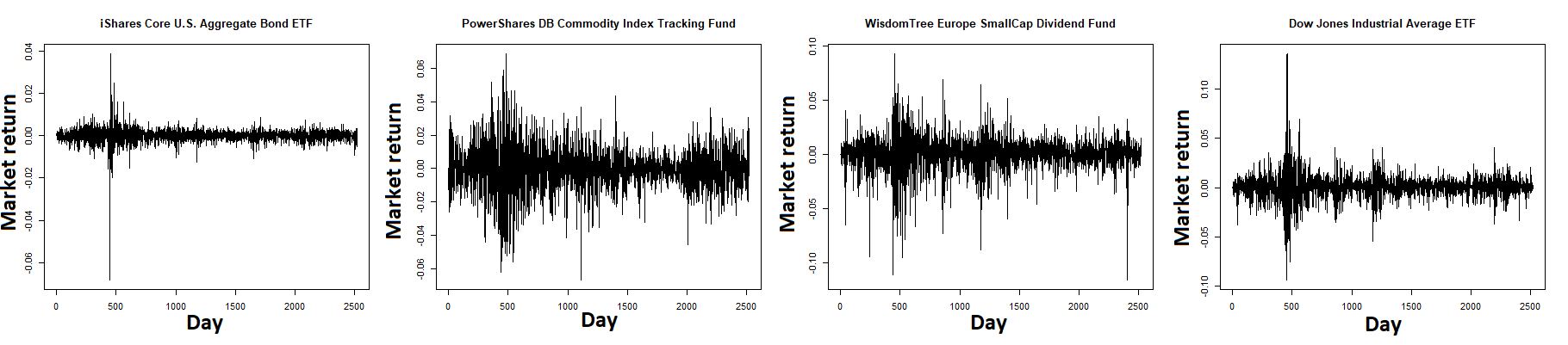
Refer to caption
Figure 4. Daily market returns of 4 different assets.

The reason for focusing solely on the value of these assets could be, for example, that they are the first available every day. The aim would be to anticipate the behavior of another asset on another market. We thus consider the return of WisdomTree Japan Hedged Equity Fund as random variable YY. The size of the sample is 2520. The first 2519 days (from January 3, 2007 to December 5, 2016) will be our learning sample, and we focus on the 2520th day, when the covariate 𝑿{\boldsymbol{X}} is 𝒙=(−0.0185%,−0.4464%,0.9614%,0.1405%){\boldsymbol{x}}=\left(-0.0185\%,-0.4464\%,0.9614\%,0.1405\%\right). Pending the opening of the second market, let us estimate the quantile of the return YY given 𝑿=𝒙{\boldsymbol{X}}={\boldsymbol{x}}.
After a brief study of the autocorrelation functions, we consider that the daily returns can be considered as independent. Concerning the shape of the data, histograms of the marginals seem symmetrical. Furthermore, the measured tail index is approximately the same for the 4 marginals. This is why suppose that the data is elliptical. After having estimated 𝝁{\boldsymbol{\mu}} and 𝚺{\boldsymbol{\Sigma}} by the method of moments, we get M⁡(𝒙)=1.072952M({\boldsymbol{x}})=1.072952. We apply our estimators η^kn\hat{\eta}_{k_{n}} and ℓ^kn,hn​(𝒙)\hat{\ell}_{k_{n},h_{n}}({\boldsymbol{x}}) given in Equations (3.3) and (3.10). We take as sequences kn=n0.6k_{n}=n^{0.6} (b=0.6b=0.6) and hn=n−0.2h_{n}=n^{-0.2} (c=0.2c=0.2), and as kernel KK the gaussian p.d.f, hence we deduce the asymptotic confidence bounds from Equation (3.14). We then obtain η^kn=2.617846\hat{\eta}_{k_{n}}=2.617846 and ℓ^kn,hn​(𝒙)=6.44334\hat{\ell}_{k_{n},h_{n}}({\boldsymbol{x}})=6.44334. Let us now estimate the high quantile qαn​(Y|𝑿=𝒙)q_{\alpha_{n}}\left(Y|{\boldsymbol{X}}={\boldsymbol{x}}\right) with level αn=1−n−a\alpha_{n}=1-n^{-a}, a>1a>1. In order to minimize the asymptotic variance of Equation (4.11), we chose a=(1−b)​(γ^kn+1)=1.047146a=(1-b)\left(\hat{\gamma}_{k_{n}}+1\right)=1.047146. By applying estimator (4.7), we get a quantile of level 0.99972560.9997256 close to 3.744985%3.744985\% for Y|𝑿=𝒙Y|{\boldsymbol{X}}={\boldsymbol{x}}. In other words, before the opening of the second market, we consider that given the returns of our first four assets, that of WisdomTree Japan Hedged Equity Fund has a probability 0.99972560.9997256 of beeing less than 3.744985%3.744985\%. For information, the true return that day was 0.7141%0.7141\%.

8. Conclusion

In this paper, we propose two estimators ℓ^kn,hn​(𝒙)\hat{\ell}_{k_{n},h_{n}}({\boldsymbol{x}}) and η^kn\hat{\eta}_{k_{n}} respectively for extremal parameters ℓ⁡(𝒙)\ell({\boldsymbol{x}}) and η\eta introduced in Equation (2.13). We have proved their consistency and asymptotic normality according to the asymptotic relationships between the sequences knk_{n} and hnh_{n}. Using these estimators, we have defined estimators for intermediate and high quantiles, proved their consistency, given their asymptotic normality under stronger conditions, and deduced estimators for extreme Lp−L_{p}-quantiles and Haezendonck-Goovaerts risk measures. Consistency and asymptotic normality are also provided for these estimators, under conditions. We have also illustrated with a numerical example the performance of our estimators, and applied them to real data set.
As working perspectives, we intend to propose a method of optimal choice of the sequences knk_{n} and hnh_{n}, which is not totally discussed in this paper. Furthermore, the shape of ℓ⁡(𝒙)\ell({\boldsymbol{x}}) and η\eta leaving Assumption 1 is a current research topic. More generally, the asymptotic relationships between conditional and unconditional quantile in other maximum domains of attraction, using for example the results of Hashorva, 2007a (), may be developed. However, we need a second-order refinement, as we need a second-order refinement of Equation (2.14) to propose asymptotic normalities 4.6 and 4.11 under weaker assumptions than Assumption 4.4. Finally, it seems that the ratio of the two terms in Equation (2.14) tends to 1 more and more slowly when the covariate vector size NN becomes large. Then, our estimation approach may perform poorly if NN is tall. This is why it might be wise to propose another method when the covariate vector size NN is large.

Appendix

Proof of Lemma 2.1

  1. (i)

    Since R1​=𝑑​χ1​ξR_{1}\overset{d}{=}\chi_{1}\xi, where χ1\chi_{1} has a Lebesgue density 2π​e−x22\sqrt{\frac{2}{\pi}}e^{-\frac{x^{2}}{2}}. According to Lemma 4.3 in Jessen and Mikosch, (2006), ξ\xi satisfies F¯ξ​(t​ω)/F¯ξ​(t)→ω−1γ\bar{F}_{\xi}(t\omega)/\bar{F}_{\xi}(t)\rightarrow\omega^{-\frac{1}{\gamma}} as t→+∞t\rightarrow+\infty. Furthermore, Lemma 4.2 in Jessen and Mikosch, (2006) entails

    ℙ⁡(ξ>t)​∼t→+∞​𝔼​[χ11γ]−1​ℙ​(R1>t).\mathbb{P}\left(\xi>t\right)\underset{t\rightarrow+\infty}{\sim}\mathbb{E}\left[\chi_{1}^{\frac{1}{\gamma}}\right]^{-1}\mathbb{P}\left(R_{1}>t\right).

    Assumption 1 provides ℙ⁡(R1>t)∼λ​t−1γ\mathbb{P}(R_{1}>t)\sim\lambda t^{-\frac{1}{\gamma}}, hence the result.

  2. (ii)

    Using again Lemma 4.2 in Jessen and Mikosch, (2006) for Rd​=𝑑​χd​ξR_{d}\overset{d}{=}\chi_{d}\xi, it comes immediatly

    ℙ⁡(Rd>t)​∼t→+∞​𝔼​[χd1γ]​ℙ​(ξ>t).\mathbb{P}\left(R_{d}>t\right)\underset{t\rightarrow+\infty}{\sim}\mathbb{E}\left[\chi_{d}^{\frac{1}{\gamma}}\right]\mathbb{P}\left(\xi>t\right).

    Some straightforward calculations provide 𝔼⁡[χd1γ]=21γ​Γ⁡(d+γ−12)Γ⁡(d2)\mathbb{E}\left[\chi_{d}^{\frac{1}{\gamma}}\right]=2^{\frac{1}{\gamma}}\frac{\Gamma\left(\frac{d+\gamma^{-1}}{2}\right)}{\Gamma\left(\frac{d}{2}\right)}.

  3. (iii)

    From (ii), we have, for all d∈ℕd\in\mathbb{N}, fRd​(t)​∼t→+∞​21γ​Γ⁡(d+γ−12)Γ⁡(d2)​λ′​t−1γ−1f_{R_{d}}(t)\underset{t\rightarrow+\infty}{\sim}2^{\frac{1}{\gamma}}\frac{\Gamma\left(\frac{d+\gamma^{-1}}{2}\right)}{\Gamma\left(\frac{d}{2}\right)}\lambda^{\prime}t^{-\frac{1}{\gamma}-1}, where λ′∈ℝ\lambda^{\prime}\in\mathbb{R} is not related to dd. The result is immediate with this expression. □\Box

Proof of Proposition 2.12

The conditional density (Proposition 3 in Maume-Deschamps et al., (2017)) leads to :

limt→∞​Φ¯R∗​(t)Φ¯R​(tη)=limt→∞​cN+1​gN+1​(M⁡(𝒙)+t2)cN​gN​(M⁡(𝒙))​η​tη−1​c1​g1​(t2​η)=limt→∞​Γ⁡(N+12)​(M⁡(𝒙)+t2)−N2πN+12​cN​gN​(M⁡(𝒙))​η​tη−1​fRN+1​(M⁡(𝒙)+t2)fR1​(tη).\underset{t\rightarrow\infty}{\lim}\frac{\bar{\Phi}_{R^{*}}(t)}{\bar{\Phi}_{R}(t^{\eta})}=\underset{t\rightarrow\infty}{\lim}\frac{c_{N+1}g_{N+1}(M({\boldsymbol{x}})+t^{2})}{c_{N}g_{N}\left(M({\boldsymbol{x}})\right)\eta t^{\eta-1}c_{1}g_{1}(t^{2\eta})}=\underset{t\rightarrow\infty}{\lim}\frac{\Gamma\left(\frac{N+1}{2}\right)(M({\boldsymbol{x}})+t^{2})^{-\frac{N}{2}}}{\pi^{\frac{N+1}{2}}c_{N}g_{N}\left(M({\boldsymbol{x}})\right)\eta t^{\eta-1}}\frac{f_{R_{N+1}}\left(\sqrt{M({\boldsymbol{x}})+t^{2}}\right)}{f_{R_{1}}(t^{\eta})}.

Using Equation (2.11) of Lemma 2.1, it comes

Φ¯R∗​(t)Φ¯R​(tη)​∼t→+∞​1πN2​cN​gN​(M⁡(𝒙))​η​Γ⁡(N+1+γ−12)Γ⁡(1+γ−12)​t(η−1)​(γ−1+1)+1−η−N.\frac{\bar{\Phi}_{R^{*}}(t)}{\bar{\Phi}_{R}(t^{\eta})}\underset{t\rightarrow+\infty}{\sim}\frac{1}{\pi^{\frac{N}{2}}c_{N}g_{N}\left(M({\boldsymbol{x}})\right)\eta}\frac{\Gamma\left(\frac{N+1+\gamma^{-1}}{2}\right)}{\Gamma\left(\frac{1+\gamma^{-1}}{2}\right)}t^{(\eta-1)(\gamma^{-1}+1)+1-\eta-N}.

Obviously, we impose 0<ℓ⁡(𝒙)<+∞0<\ell({\boldsymbol{x}})<+\infty, then 1−η−N+(η−1)​(γ−1+1)=01-\eta-N+(\eta-1)(\gamma^{-1}+1)=0, hence η=N​γ+1\eta=N\gamma+1. Replacing η\eta in the previous equation, ℓ⁡(𝒙)\ell({\boldsymbol{x}}) is easily deduced :

ℓ(𝒙)=1πN2​cN​gN​(M⁡(𝒙))​ηΓ⁡(N+1+γ−12)Γ⁡(1+γ−12). □\ell({\boldsymbol{x}})=\frac{1}{\pi^{\frac{N}{2}}c_{N}g_{N}\left(M({\boldsymbol{x}})\right)\eta}\frac{\Gamma\left(\frac{N+1+\gamma^{-1}}{2}\right)}{\Gamma\left(\frac{1+\gamma^{-1}}{2}\right)}.\text{ }\Box

Proof of Proposition 3.13

It is obvious that under conditions (K​1)−(K​2)(K1)-(K2), kn​(g^hn−cN​gN​(M⁡(𝒙)))​→ℙ​0\sqrt{k_{n}}\left(\hat{g}_{h_{n}}-c_{N}g_{N}\left(M({\boldsymbol{x}})\right)\right)\overset{\mathbb{P}}{\rightarrow}0 as n→+∞n\rightarrow+\infty if kn=o⁡(n​hn)k_{n}=o(nh_{n}) and kn​hn2→0\sqrt{k_{n}}h_{n}^{2}\rightarrow 0. Then we get the following asymptotic normality :

kn​(γ^kn−γg^hn−cN​gN​(M⁡(𝒙)))​→n→+∞​𝒩​((00),(γ2000)).\sqrt{k_{n}}\begin{pmatrix}\hat{\gamma}_{k_{n}}-\gamma\\ \hat{g}_{h_{n}}-c_{N}g_{N}\left(M({\boldsymbol{x}})\right)\end{pmatrix}\underset{n\rightarrow+\infty}{\rightarrow}\mathcal{N}\left(\begin{pmatrix}0\\ 0\end{pmatrix},\begin{pmatrix}\gamma^{2}&0\\ 0&0\end{pmatrix}\right).

Since ℓ⁡(𝒙)=u⁡(γ)\ell({\boldsymbol{x}})=u(\gamma), the delta method entails

kn​(ℓ^kn,hn​(𝒙)−ℓ⁡(𝒙))​→n→+∞​𝒩​(0,u′​(γ)2​γ2).\sqrt{k_{n}}\left(\hat{\ell}_{k_{n},h_{n}}({\boldsymbol{x}})-\ell({\boldsymbol{x}})\right)\underset{n\rightarrow+\infty}{\rightarrow}\mathcal{N}\left(0,u^{\prime}(\gamma)^{2}\gamma^{2}\right).

A quick calculation of u′u^{\prime}, using Equation (2.12), gives the first result. The second part of the proof is similar. Indeed, if n​hn=o⁡(kn)nh_{n}=o(k_{n}) and n​hn5→0nh_{n}^{5}\rightarrow 0 as n→+∞n\rightarrow+\infty, then

n​hn​(γ^kn−γg^hn−cN​gN​(M⁡(𝒙)))​→n→+∞​𝒩​((00),(000M​(𝒙)1−N2​Γ​(N2)πN2​cN​gN​(M⁡(𝒙))​∫K​(u)2​𝑑u)).\sqrt{nh_{n}}\begin{pmatrix}\hat{\gamma}_{k_{n}}-\gamma\\ \hat{g}_{h_{n}}-c_{N}g_{N}\left(M({\boldsymbol{x}})\right)\end{pmatrix}\underset{n\rightarrow+\infty}{\rightarrow}\mathcal{N}\left(\begin{pmatrix}0\\ 0\end{pmatrix},\begin{pmatrix}0&0\\ 0&\frac{M({\boldsymbol{x}})^{1-\frac{N}{2}}\Gamma\left(\frac{N}{2}\right)}{\pi^{\frac{N}{2}}}c_{N}g_{N}\left(M({\boldsymbol{x}})\right)\int K(u)^{2}du\end{pmatrix}\right).

The delta method completes the proof. □\Box

In order to make the proof of Theorem 4.3 easier to read, we give the following lemma, which provides the asymptotic behavior of a statistic order under Assumption 1.

Lemma 8.1.

Under Assumption 1 and condition (C)(C),

(8.1) n​vn​((W[n​vn+1])ΦR−1​(1−vn)−1)​→n→+∞​𝒩​(0,γ2).\sqrt{nv_{n}}\left(\frac{\left(W_{[nv_{n}+1]}\right)}{\Phi_{R}^{-1}\left(1-v_{n}\right)}-1\right)\underset{n\rightarrow+\infty}{\rightarrow}\mathcal{N}\left(0,\gamma^{2}\right).

Proof of Lemma 8.1

The proof is inspired by Theorem 2.4.1 in de Haan and Ferreira, (2006). Let Y1,Y2,…Y_{1},Y_{2},\ldots be independant and identically distributed random variables with c.d.f. 1−y−1,y>11-y^{-1},y>1. We denote in addition Y[n]≤…≤Y[1]Y_{[n]}\leq\ldots\leq Y_{[1]}. We thus have

n​vn​(vn​Y[n​vn+1]−1)​→n→+∞​𝒩​(0,1).\sqrt{nv_{n}}\left(v_{n}Y_{[nv_{n}+1]}-1\right)\underset{n\rightarrow+\infty}{\rightarrow}\mathcal{N}(0,1).

By noticing that W[n​vn+1]​=𝑑​ΦR−1​(1−1/Y[n​vn+1])W_{[nv_{n}+1]}\overset{d}{=}\Phi_{R}^{-1}\left(1-1/Y_{[nv_{n}+1]}\right), it comes

n​vn​((W[n​vn+1])ΦR−1​(1−vn)−1)​=𝑑​n​vn​(ΦR−1​(1−1/Y[n​vn+1])ΦR−1​(1−vn)−(vn​Y[n​vn+1])γ)+n​vn​((vn​Y[n​vn+1])γ−1).\sqrt{nv_{n}}\left(\frac{\left(W_{[nv_{n}+1]}\right)}{\Phi_{R}^{-1}\left(1-v_{n}\right)}-1\right)\overset{d}{=}\sqrt{nv_{n}}\left(\frac{\Phi_{R}^{-1}\left(1-1/Y_{[nv_{n}+1]}\right)}{\Phi_{R}^{-1}\left(1-v_{n}\right)}-\left(v_{n}Y_{[nv_{n}+1]}\right)^{\gamma}\right)+\sqrt{nv_{n}}\left(\left(v_{n}Y_{[nv_{n}+1]}\right)^{\gamma}-1\right).

The delta method entails that the second term tends to 𝒩⁡(0,γ2)\mathcal{N}(0,\gamma^{2}). Moreover, Assumption 1 and kn​A​(nkn)→0\sqrt{k_{n}}A\left(\frac{n}{k_{n}}\right)\rightarrow 0 as n→+∞n\rightarrow+\infty ensure the asymptotic nullity of the first term.

Proof of Theorem 4.3

In a first time, we can notice v~n\tilde{v}_{n} is related to ℓ^kn,hn​(𝒙)\hat{\ell}_{k_{n},h_{n}}({\boldsymbol{x}}). Then, according to Proposition 3.13, (i) entails that we can deal with vnv_{n} instead of v~n\tilde{v}_{n} in Equation (4.2). Furthermore, we give the decomposition :

(8.2) knln⁡(1−αn)​(q^αn​(Y|𝑿=𝒙)qαn↑​(Y|𝑿=𝒙)−1)​∼n→+∞​knln⁡(1−αn)​((W[n​vn+1])1/η^knΦR−1​(1−vn)1/η−1)=knln⁡(1−αn)​((W[n​vn+1])1/η^knΦR−1​(1−vn)1/η^kn−1)​ΦR−1​(1−vn)1/η^kn−1/η+knln⁡(1−αn)​(ΦR−1​(1−vn)1/η^kn−1/η−1).\frac{\sqrt{k_{n}}}{\ln\left(1-\alpha_{n}\right)}\left(\frac{\hat{q}_{\alpha_{n}}\left(Y|{\boldsymbol{X}}={\boldsymbol{x}}\right)}{q_{\alpha_{n}\uparrow}\left(Y|{\boldsymbol{X}}={\boldsymbol{x}}\right)}-1\right)\underset{n\rightarrow+\infty}{\sim}\frac{\sqrt{k_{n}}}{\ln\left(1-\alpha_{n}\right)}\left(\frac{\left(W_{[nv_{n}+1]}\right)^{1/\hat{\eta}_{k_{n}}}}{\Phi_{R}^{-1}\left(1-v_{n}\right)^{1/\eta}}-1\right)=\\ \frac{\sqrt{k_{n}}}{\ln\left(1-\alpha_{n}\right)}\left(\frac{\left(W_{[nv_{n}+1]}\right)^{1/\hat{\eta}_{k_{n}}}}{\Phi_{R}^{-1}\left(1-v_{n}\right)^{1/\hat{\eta}_{k_{n}}}}-1\right)\Phi_{R}^{-1}\left(1-v_{n}\right)^{1/\hat{\eta}_{k_{n}}-1/\eta}+\frac{\sqrt{k_{n}}}{\ln\left(1-\alpha_{n}\right)}\left(\Phi_{R}^{-1}\left(1-v_{n}\right)^{1/\hat{\eta}_{k_{n}}-1/\eta}-1\right).

Under Assumption 1, and according to Proposition 3.4 and Theorem 2.4.1 in de Haan and Ferreira, (2006) (with (C)(C)), we have :

{kn​(1η^kn−1η)→n→+∞​𝒩​(0,N2​γ2(γ​N+1)4)n​vn​((W[n​vn+1])ΦR−1​(1−vn)−1)→n→+∞​𝒩​(0,γ2),\left\{\begin{array}[]{cc}\sqrt{k_{n}}\left(\frac{1}{\hat{\eta}_{k_{n}}}-\frac{1}{\eta}\right)&\underset{n\rightarrow+\infty}{\rightarrow}\mathcal{N}\left(0,\frac{N^{2}\gamma^{2}}{\left(\gamma N+1\right)^{4}}\right)\\ \sqrt{nv_{n}}\left(\frac{\left(W_{[nv_{n}+1]}\right)}{\Phi_{R}^{-1}\left(1-v_{n}\right)}-1\right)&\underset{n\rightarrow+\infty}{\rightarrow}\mathcal{N}\left(0,\gamma^{2}\right)\\ \end{array}\right.,

By noticing that vnv_{n} is equivalent to ℓ​(𝒙)−1​(1−αn)\ell({\boldsymbol{x}})^{-1}(1-\alpha_{n}) as n→+∞n\rightarrow+\infty, and using condition kn=o⁡(ln⁡(1−αn)​n⁡(1−αn))\sqrt{k_{n}}=o\left(\ln(1-\alpha_{n})\sqrt{n(1-\alpha_{n})}\right) in (Ci​n​t)(C_{int}), it comes

knln⁡(1−αn)​((W[n​vn+1])1/η^knΦR−1​(1−vn)1/η^kn−1)→0​ as ​n→+∞.\frac{\sqrt{k_{n}}}{\ln\left(1-\alpha_{n}\right)}\left(\frac{\left(W_{[nv_{n}+1]}\right)^{1/\hat{\eta}_{k_{n}}}}{\Phi_{R}^{-1}\left(1-v_{n}\right)^{1/\hat{\eta}_{k_{n}}}}-1\right)\rightarrow 0\text{ as }n\rightarrow+\infty.

Furthermore, under Assumption 1, ln⁡(ΦR−1​(1−vn))\ln\left(\Phi_{R}^{-1}(1-v_{n})\right) is cleary equivalent to −γ​ln⁡(vn)-\gamma\ln(v_{n}), or −γ​ln⁡(1−αn)-\gamma\ln(1-\alpha_{n}). Then (Ci​n​t)(C_{int}) ensures ΦR−1​(1−vn)1/η^kn−1/η→1\Phi_{R}^{-1}\left(1-v_{n}\right)^{1/\hat{\eta}_{k_{n}}-1/\eta}\rightarrow 1 as n→+∞n\rightarrow+\infty, and therefore the first term of the decomposition tends to 0. It thus remains to calculate the limit of the second term. It is not complicated to notice that

knln⁡(ΦR−1​(1−vn))​(ΦR−1​(1−vn)1/η^kn−1/η−1)​→n→+∞​𝒩​(0,N2​γ2(γ​N+1)4).\frac{\sqrt{k_{n}}}{\ln\left(\Phi_{R}^{-1}\left(1-v_{n}\right)\right)}\left(\Phi_{R}^{-1}\left(1-v_{n}\right)^{1/\hat{\eta}_{k_{n}}-1/\eta}-1\right)\underset{n\rightarrow+\infty}{\rightarrow}\mathcal{N}\left(0,\frac{N^{2}\gamma^{2}}{\left(\gamma N+1\right)^{4}}\right).

Using the equivalence ln⁡(ΦR−1​(1−vn))∼−γ​ln⁡(vn)∼−γ​ln⁡(1−αn)\ln\left(\Phi_{R}^{-1}(1-v_{n})\right)\sim-\gamma\ln(v_{n})\sim-\gamma\ln(1-\alpha_{n}), we get the result (4.2). Using asymptotic relationship (2.14), the consistency 4.3 is obvious. □\Box

Proof of Proposition 4.6

We recall that density of ΦR∗\Phi_{R^{*}} is proportional to cN+1​gN+1​(M⁡(𝒙)+t2)c_{N+1}g_{N+1}\left(M({\boldsymbol{x}})+t^{2}\right), and, from Assumption 4.4, there exist λ1,λ2∈ℝ\lambda_{1},\lambda_{2}\in\mathbb{R} such that :

cN+1​gN+1​(M⁡(𝒙)+t2)=λ1​(M⁡(𝒙)+t2)−N+1+γ−12​[1+λ2​(M⁡(𝒙)+t2)ρ2​γ+o⁡(tργ)]c_{N+1}g_{N+1}\left(M({\boldsymbol{x}})+t^{2}\right)=\lambda_{1}\left(M({\boldsymbol{x}})+t^{2}\right)^{-\frac{N+1+\gamma^{-1}}{2}}\left[1+\lambda_{2}\left(M({\boldsymbol{x}})+t^{2}\right)^{\frac{\rho}{2\gamma}}+o\left(t^{\frac{\rho}{\gamma}}\right)\right]

The previous expression may be rewritten as follows, where λ1,λ2,λ3∈ℝ\lambda_{1},\lambda_{2},\lambda_{3}\in\mathbb{R} :

cN+1​gN+1​(M⁡(𝒙)+t2)=λ1​t−(N+1+γ−1)​[1+λ2​(M⁡(𝒙)+t2)ρ2​γ+λ3​t−2+o⁡(tργ)]c_{N+1}g_{N+1}\left(M({\boldsymbol{x}})+t^{2}\right)=\lambda_{1}t^{-(N+1+\gamma^{-1})}\left[1+\lambda_{2}\left(M({\boldsymbol{x}})+t^{2}\right)^{\frac{\rho}{2\gamma}}+\lambda_{3}t^{-2}+o\left(t^{\frac{\rho}{\gamma}}\right)\right]

In order to make the proof more readable, we do not specify the values of constants λi\lambda_{i}, because they are not essential. Then, in the case, ρ/γ≤−2\rho/\gamma\leq-2, we get

cN+1​gN+1​(M⁡(𝒙)+t2)=λ1​t−(N+1+γ−1)​[1+λ2​t−2+o⁡(t−2)],λ1,λ2∈ℝc_{N+1}g_{N+1}\left(M({\boldsymbol{x}})+t^{2}\right)=\lambda_{1}t^{-(N+1+\gamma^{-1})}\left[1+\lambda_{2}t^{-2}+o\left(t^{-2}\right)\right],\lambda_{1},\lambda_{2}\in\mathbb{R}

In other terms, cN+1​gN+1​(M⁡(𝒙)+t2)c_{N+1}g_{N+1}\left(M({\boldsymbol{x}})+t^{2}\right) is regularly varying of second order with indices −N−1−γ−1-N-1-\gamma^{-1}, −2-2, and an auxiliary function propotional to t−2t^{-2}. According to Proposition 6 of Hua and Joe, (2011), Φ¯R∗​(t)=∫t+∞cN+1​gN+1​(M⁡(𝒙)+u2)​𝑑u∈2​R​V−N−γ−1,−2\bar{\Phi}_{R^{*}}(t)=\int_{t}^{+\infty}c_{N+1}g_{N+1}\left(M({\boldsymbol{x}})+u^{2}\right)du\in 2RV_{-N-\gamma^{-1},-2} with an auxiliary function proportional to t−2t^{-2}. Equivalently, there exists λ1,λ2∈ℝ\lambda_{1},\lambda_{2}\in\mathbb{R} such that

ΦR∗−1​(1−1t)=λ1​tγγ​N+1​[1+λ2​t−2​γγ​N+1+o⁡(t−2​γγ​N+1)].\Phi_{R^{*}}^{-1}\left(1-\frac{1}{t}\right)=\lambda_{1}t^{\frac{\gamma}{\gamma N+1}}\left[1+\lambda_{2}t^{-\frac{2\gamma}{\gamma N+1}}+o\left(t^{-\frac{2\gamma}{\gamma N+1}}\right)\right].

Since Assumption 1 and Assumption 4.4 provide ΦR−1​(1−1/t)=λ3​tγ​[1+λ4​tρ+o⁡(tρ)]\Phi_{R}^{-1}(1-1/t)=\lambda_{3}t^{\gamma}\left[1+\lambda_{4}t^{\rho}+o\left(t^{\rho}\right)\right], it comes

ΦR−1​(1−vn)1ηΦR∗−1​(αn)=ℓ​(𝒙)−γγ​N+1​(1−αnvn)γγ​N+1​1+λ1​vn−ρ+o⁡(vn−ρ)1+λ2​(1−αn)2​γγ​N+1+o⁡((1−αn)2​γγ​N+1),\frac{\Phi_{R}^{-1}\left(1-v_{n}\right)^{\frac{1}{\eta}}}{\Phi_{R^{*}}^{-1}(\alpha_{n})}=\ell({\boldsymbol{x}})^{-\frac{\gamma}{\gamma N+1}}\left(\frac{1-\alpha_{n}}{v_{n}}\right)^{\frac{\gamma}{\gamma N+1}}\frac{1+\lambda_{1}v_{n}^{-\rho}+o\left(v_{n}^{-\rho}\right)}{1+\lambda_{2}(1-\alpha_{n})^{\frac{2\gamma}{\gamma N+1}}+o\left((1-\alpha_{n})^{\frac{2\gamma}{\gamma N+1}}\right)},

for some constants λ1,λ2∈ℝ\lambda_{1},\lambda_{2}\in\mathbb{R}. In that case, we considered ρ≤−2​γ\rho\leq-2\gamma, hence −ρ>2​γ/(γ​N+1)-\rho>2\gamma/(\gamma N+1). We then deduce the following expansion :

ΦR−1​(1−vn)1ηΦR∗−1​(αn)=ℓ​(𝒙)−γγ​N+1​(1−αnvn)γγ​N+1​[1+λ​(1−αn)2​γγ​N+1+o⁡((1−αn)2​γγ​N+1)],\frac{\Phi_{R}^{-1}\left(1-v_{n}\right)^{\frac{1}{\eta}}}{\Phi_{R^{*}}^{-1}(\alpha_{n})}=\ell({\boldsymbol{x}})^{-\frac{\gamma}{\gamma N+1}}\left(\frac{1-\alpha_{n}}{v_{n}}\right)^{\frac{\gamma}{\gamma N+1}}\left[1+\lambda(1-\alpha_{n})^{\frac{2\gamma}{\gamma N+1}}+o\left((1-\alpha_{n})^{\frac{2\gamma}{\gamma N+1}}\right)\right],

for a certain constant λ∈ℝ\lambda\in\mathbb{R}. We can notice that (1−αn)/vn=2​(1−ℓ⁡(𝒙))​(1−αn)+ℓ⁡(𝒙)(1-\alpha_{n})/v_{n}=2(1-\ell({\boldsymbol{x}}))(1-\alpha_{n})+\ell({\boldsymbol{x}}), and let us now focus on the limit :

(8.3) limn→+∞ knln⁡(1−αn)ln(ΦR−1​(1−vn)1ηΦR∗−1​(αn))=γγ​N+1limn→+∞ knln⁡(1−αn)ln(21−ℓ⁡(𝒙)ℓ⁡(𝒙)(1−αn)+1)+limn→+∞ knln⁡(1−αn)ln(1+λ(1−αn)2​γγ​N+1+o((1−αn)2​γγ​N+1)).\underset{n\rightarrow+\infty}{\lim}\text{ }\frac{\sqrt{k_{n}}}{\ln\left(1-\alpha_{n}\right)}\ln\left(\frac{\Phi_{R}^{-1}\left(1-v_{n}\right)^{\frac{1}{\eta}}}{\Phi_{R^{*}}^{-1}(\alpha_{n})}\right)=\frac{\gamma}{\gamma N+1}\underset{n\rightarrow+\infty}{\lim}\text{ }\frac{\sqrt{k_{n}}}{\ln\left(1-\alpha_{n}\right)}\ln\left(2\frac{1-\ell({\boldsymbol{x}})}{\ell({\boldsymbol{x}})}(1-\alpha_{n})+1\right)\\ +\underset{n\rightarrow+\infty}{\lim}\text{ }\frac{\sqrt{k_{n}}}{\ln\left(1-\alpha_{n}\right)}\ln\left(1+\lambda(1-\alpha_{n})^{\frac{2\gamma}{\gamma N+1}}+o\left((1-\alpha_{n})^{\frac{2\gamma}{\gamma N+1}}\right)\right).

The first term gives is easy to calculate. Indeed, since kn​(1−αn)/ln⁡(1−αn)→0\sqrt{k_{n}}(1-\alpha_{n})/\ln\left(1-\alpha_{n}\right)\rightarrow 0 as n→+∞n\rightarrow+\infty, we deduce

limn→+∞ knln⁡(1−αn)ln(21−ℓ⁡(𝒙)ℓ⁡(𝒙)(1−αn)+1)=21−ℓ⁡(𝒙)ℓ⁡(𝒙)limn→+∞ knln⁡(1−αn)(1−αn)=0.\underset{n\rightarrow+\infty}{\lim}\text{ }\frac{\sqrt{k_{n}}}{\ln\left(1-\alpha_{n}\right)}\ln\left(2\frac{1-\ell({\boldsymbol{x}})}{\ell({\boldsymbol{x}})}(1-\alpha_{n})+1\right)=2\frac{1-\ell({\boldsymbol{x}})}{\ell({\boldsymbol{x}})}\underset{n\rightarrow+\infty}{\lim}\text{ }\frac{\sqrt{k_{n}}}{\ln\left(1-\alpha_{n}\right)}(1-\alpha_{n})=0.

By a similar calculation, the second term also tends to 0, supposing knln⁡(1−αn)​(1−αn)2​γγ​N+1→0\frac{\sqrt{k_{n}}}{\ln\left(1-\alpha_{n}\right)}\left(1-\alpha_{n}\right)^{\frac{2\gamma}{\gamma N+1}}\rightarrow 0 as n→+∞n\rightarrow+\infty. Then, we deduce, using Proposition 4.3 :

(8.4) knln⁡(1−αn)​(q^αn​(Y|𝑿=𝒙)qαn​(Y|𝑿=𝒙)−1)∼knln⁡(1−αn)​((W[n​vn+1])1/η^knΦR∗−1​(αn)−1)=knln⁡(1−αn)​(q^αn​(R∗​U(1))ΦR−1​(1−vn)1η−1)​ΦR−1​(1−vn)1ηΦR∗−1​(αn)+knln⁡(1−αn)​(ΦR−1​(1−vn)1ηΦR∗−1​(αn)−1)​→n→+∞​𝒩​(0,N2​γ4(γ​N+1)4).\frac{\sqrt{k_{n}}}{\ln\left(1-\alpha_{n}\right)}\left(\frac{\hat{q}_{\alpha_{n}}\left(Y|{\boldsymbol{X}}={\boldsymbol{x}}\right)}{q_{\alpha_{n}}\left(Y|{\boldsymbol{X}}={\boldsymbol{x}}\right)}-1\right)\sim\frac{\sqrt{k_{n}}}{\ln\left(1-\alpha_{n}\right)}\left(\frac{\left(W_{[nv_{n}+1]}\right)^{1/\hat{\eta}_{k_{n}}}}{\Phi_{R^{*}}^{-1}\left(\alpha_{n}\right)}-1\right)=\\ \frac{\sqrt{k_{n}}}{\ln\left(1-\alpha_{n}\right)}\left(\frac{\hat{q}_{\alpha_{n}}\left(R^{*}U^{(1)}\right)}{\Phi_{R}^{-1}\left(1-v_{n}\right)^{\frac{1}{\eta}}}-1\right)\frac{\Phi_{R}^{-1}\left(1-v_{n}\right)^{\frac{1}{\eta}}}{\Phi_{R^{*}}^{-1}(\alpha_{n})}+\frac{\sqrt{k_{n}}}{\ln\left(1-\alpha_{n}\right)}\left(\frac{\Phi_{R}^{-1}\left(1-v_{n}\right)^{\frac{1}{\eta}}}{\Phi_{R^{*}}^{-1}(\alpha_{n})}-1\right)\underset{n\rightarrow+\infty}{\rightarrow}\mathcal{N}\left(0,\frac{N^{2}\gamma^{4}}{\left(\gamma N+1\right)^{4}}\right).

Now, let us focus on the case ρ/γ>−2\rho/\gamma>-2. The proof is exactly the same, with

cN+1​gN+1​(M⁡(𝒙)+t2)=λ1​t−(N+1+γ−1)​[1+λ2​tργ+o⁡(tργ)],λ1,λ2∈ℝ.c_{N+1}g_{N+1}\left(M({\boldsymbol{x}})+t^{2}\right)=\lambda_{1}t^{-(N+1+\gamma^{-1})}\left[1+\lambda_{2}t^{\frac{\rho}{\gamma}}+o\left(t^{\frac{\rho}{\gamma}}\right)\right],\lambda_{1},\lambda_{2}\in\mathbb{R}.

Using the same calculations and doing the further assumption limn→+∞​knln⁡(1−αn)​(1−αn)−ργ​N+1=0\underset{n\rightarrow+\infty}{\lim}\frac{\sqrt{k_{n}}}{\ln\left(1-\alpha_{n}\right)}\left(1-\alpha_{n}\right)^{-\frac{\rho}{\gamma N+1}}=0 leads to the result. □\Box

Proof of Theorem 4.9

Firstly, we can notice that

(8.5) q^^αn​(Y|𝑿=𝒙)qαn↑​(Y|𝑿=𝒙)−1​∼n→+∞​[W[kn+1]​(knn​v~n)γ^kn]1η^knΦR−1​(1−vn)1η−1=([W[kn+1]​(knn​vn)γ^kn]1η^knΦR−1​(1−vn)1η−1)​(vnv~n)γ^knη^kn+(vnv~n)γ^knη^kn−1.\frac{\hat{\hat{q}}_{\alpha_{n}}\left(Y|{\boldsymbol{X}}={\boldsymbol{x}}\right)}{q_{\alpha_{n}\uparrow}\left(Y|{\boldsymbol{X}}={\boldsymbol{x}}\right)}-1\underset{n\rightarrow+\infty}{\sim}\frac{\left[W_{[k_{n}+1]}\left(\frac{k_{n}}{n\tilde{v}_{n}}\right)^{\hat{\gamma}_{k_{n}}}\right]^{\frac{1}{\hat{\eta}_{k_{n}}}}}{\Phi_{R}^{-1}\left(1-v_{n}\right)^{\frac{1}{\eta}}}-1=\\ \left(\frac{\left[W_{[k_{n}+1]}\left(\frac{k_{n}}{nv_{n}}\right)^{\hat{\gamma}_{k_{n}}}\right]^{\frac{1}{\hat{\eta}_{k_{n}}}}}{\Phi_{R}^{-1}\left(1-v_{n}\right)^{\frac{1}{\eta}}}-1\right)\left(\frac{v_{n}}{\tilde{v}_{n}}\right)^{\frac{\hat{\gamma}_{k_{n}}}{\hat{\eta}_{k_{n}}}}+\left(\frac{v_{n}}{\tilde{v}_{n}}\right)^{\frac{\hat{\gamma}_{k_{n}}}{\hat{\eta}_{k_{n}}}}-1.

Since kn=o⁡(n​hn)k_{n}=o(nh_{n}), we deduce

knln⁡(knn​vn)​([W[kn+1]​(knn​v~n)γ^kn]1η^knΦR−1​(1−vn)1η−1)​∼n→+∞​knln⁡(knn​vn)​([W[kn+1]​(knn​vn)γ^kn]1η^knΦR−1​(1−vn)1η−1).\frac{\sqrt{k_{n}}}{\ln\left(\frac{k_{n}}{nv_{n}}\right)}\left(\frac{\left[W_{[k_{n}+1]}\left(\frac{k_{n}}{n\tilde{v}_{n}}\right)^{\hat{\gamma}_{k_{n}}}\right]^{\frac{1}{\hat{\eta}_{k_{n}}}}}{\Phi_{R}^{-1}\left(1-v_{n}\right)^{\frac{1}{\eta}}}-1\right)\underset{n\rightarrow+\infty}{\sim}\frac{\sqrt{k_{n}}}{\ln\left(\frac{k_{n}}{nv_{n}}\right)}\left(\frac{\left[W_{[k_{n}+1]}\left(\frac{k_{n}}{nv_{n}}\right)^{\hat{\gamma}_{k_{n}}}\right]^{\frac{1}{\hat{\eta}_{k_{n}}}}}{\Phi_{R}^{-1}\left(1-v_{n}\right)^{\frac{1}{\eta}}}-1\right).

Furthermore, according to Theorem 4.3.8 in de Haan and Ferreira, (2006), (C)(C) and (Ch​i​g​h)(C_{high}) lead to

knln⁡(knn​vn)​(W[kn+1]​(knn​vn)γ^knΦR−1​(1−vn)−1)​∼n→+∞​knln⁡(knn​vn)​((knn​vn)γ^kn−γ−1).\frac{\sqrt{k_{n}}}{\ln\left(\frac{k_{n}}{nv_{n}}\right)}\left(\frac{W_{[k_{n}+1]}\left(\frac{k_{n}}{nv_{n}}\right)^{\hat{\gamma}_{k_{n}}}}{\Phi_{R}^{-1}\left(1-v_{n}\right)}-1\right)\underset{n\rightarrow+\infty}{\sim}\frac{\sqrt{k_{n}}}{\ln\left(\frac{k_{n}}{nv_{n}}\right)}\left(\left(\frac{k_{n}}{nv_{n}}\right)^{\hat{\gamma}_{k_{n}}-\gamma}-1\right).

From Assumption 1, it is not difficult to prove that ln⁡(ΦR−1​(1−vn))/ln⁡(kn/(n​vn))\ln\left(\Phi_{R}^{-1}(1-v_{n})\right)/\ln\left(k_{n}/(nv_{n})\right) is asymptotically equivalent to γ​ln⁡(1−αn)/ln⁡(n⁡(1−αn)/kn)\gamma\ln(1-\alpha_{n})/\ln\left(n(1-\alpha_{n})/k_{n}\right). Then, if we focus on the second term, it comes, using the limit given in (Ch​i​g​h)(C_{high}) :

knln⁡(knn​vn)​((knn​vn)γ^kn−γ−1ΦR​(1−vn)1η^kn−1η−1)​→n→+∞​𝒩​((00),(γ2−θ​N​γ3(γ​N+1)2−θ​N​γ3(γ​N+1)2θ2​N2​γ4(γ​N+1)4)).\frac{\sqrt{k_{n}}}{\ln\left(\frac{k_{n}}{nv_{n}}\right)}\begin{pmatrix}\left(\frac{k_{n}}{nv_{n}}\right)^{\hat{\gamma}_{k_{n}}-\gamma}-1\\ \Phi_{R}\left(1-v_{n}\right)^{\frac{1}{\hat{\eta}_{k_{n}}}-\frac{1}{\eta}}-1\end{pmatrix}\underset{n\rightarrow+\infty}{\rightarrow}\mathcal{N}\left(\begin{pmatrix}0\\ 0\end{pmatrix},\begin{pmatrix}\gamma^{2}&-\theta\frac{N\gamma^{3}}{(\gamma N+1)^{2}}\\ -\theta\frac{N\gamma^{3}}{(\gamma N+1)^{2}}&\theta^{2}\frac{N^{2}\gamma^{4}}{(\gamma N+1)^{4}}\end{pmatrix}\right).

Finally,

(8.6) knln⁡(knn​vn)​([W[kn+1]​(knn​v~n)γ^kn]1η^knΦR−1​(1−vn)1η−1)=knln⁡(knn​vn)​(ΦR−1​(1−vn)1η^kn−1η−1)+knln⁡(knn​vn)​([W[kn+1]​(knn​v~n)γ^kn]1η^knΦR−1​(1−vn)1η^kn−1)​ΦR−1​(1−vn)1η^kn−1η.\frac{\sqrt{k_{n}}}{\ln\left(\frac{k_{n}}{nv_{n}}\right)}\left(\frac{\left[W_{[k_{n}+1]}\left(\frac{k_{n}}{n\tilde{v}_{n}}\right)^{\hat{\gamma}_{k_{n}}}\right]^{\frac{1}{\hat{\eta}_{k_{n}}}}}{\Phi_{R}^{-1}\left(1-v_{n}\right)^{\frac{1}{\eta}}}-1\right)=\frac{\sqrt{k_{n}}}{\ln\left(\frac{k_{n}}{nv_{n}}\right)}\left(\Phi_{R}^{-1}\left(1-v_{n}\right)^{\frac{1}{\hat{\eta}_{k_{n}}}-\frac{1}{\eta}}-1\right)\\ +\frac{\sqrt{k_{n}}}{\ln\left(\frac{k_{n}}{nv_{n}}\right)}\left(\frac{\left[W_{[k_{n}+1]}\left(\frac{k_{n}}{n\tilde{v}_{n}}\right)^{\hat{\gamma}_{k_{n}}}\right]^{\frac{1}{\hat{\eta}_{k_{n}}}}}{\Phi_{R}^{-1}\left(1-v_{n}\right)^{\frac{1}{\hat{\eta}_{k_{n}}}}}-1\right)\Phi_{R}^{-1}\left(1-v_{n}\right)^{\frac{1}{\hat{\eta}_{k_{n}}}-\frac{1}{\eta}}.

When n→∞n\rightarrow\infty, this expression is the sum of the following bivariate normal distribution :

knln⁡(knn​vn)​([W[kn+1]​(knn​v~n)γ^kn]1η^knΦR−1​(1−vn)1η^kn−1ΦR​(1−vn)1η^kn−1η−1)​→n→+∞​𝒩​((00),(γ2(γ​N+1)2−θ​N​γ3(γ​N+1)3−θ​N​γ3(γ​N+1)3θ2​N2​γ4(γ​N+1)4)),\frac{\sqrt{k_{n}}}{\ln\left(\frac{k_{n}}{nv_{n}}\right)}\begin{pmatrix}\frac{\left[W_{[k_{n}+1]}\left(\frac{k_{n}}{n\tilde{v}_{n}}\right)^{\hat{\gamma}_{k_{n}}}\right]^{\frac{1}{\hat{\eta}_{k_{n}}}}}{\Phi_{R}^{-1}\left(1-v_{n}\right)^{\frac{1}{\hat{\eta}_{k_{n}}}}}-1\\ \Phi_{R}\left(1-v_{n}\right)^{\frac{1}{\hat{\eta}_{k_{n}}}-\frac{1}{\eta}}-1\end{pmatrix}\underset{n\rightarrow+\infty}{\rightarrow}\mathcal{N}\left(\begin{pmatrix}0\\ 0\end{pmatrix},\begin{pmatrix}\frac{\gamma^{2}}{(\gamma N+1)^{2}}&-\theta\frac{N\gamma^{3}}{(\gamma N+1)^{3}}\\ -\theta\frac{N\gamma^{3}}{(\gamma N+1)^{3}}&\theta^{2}\frac{N^{2}\gamma^{4}}{(\gamma N+1)^{4}}\end{pmatrix}\right),

To conclude, ln⁡(knn​vn)∼ln⁡(knn⁡(1−αn))\ln\left(\frac{k_{n}}{nv_{n}}\right)\sim\ln\left(\frac{k_{n}}{n(1-\alpha_{n})}\right) as n→+∞n\rightarrow+\infty, hence the result. The consistency is immediate. □\Box

Proof of Proposition 4.11

The proof is similar to that of Proposition 4.6. Indeed, we have given, in the case ρ/γ≤−2\rho/\gamma\leq-2 :

ΦR−1​(1−vn)1ηΦR∗−1​(αn)=ℓ​(𝒙)−γγ​N+1​(2​(1−ℓ⁡(𝒙))​(1−αn)+ℓ⁡(𝒙))γγ​N+1​[1+λ​(1−αn)2​γγ​N+1+o⁡((1−αn)2​γγ​N+1)],\frac{\Phi_{R}^{-1}\left(1-v_{n}\right)^{\frac{1}{\eta}}}{\Phi_{R^{*}}^{-1}(\alpha_{n})}=\ell({\boldsymbol{x}})^{-\frac{\gamma}{\gamma N+1}}\left(2(1-\ell({\boldsymbol{x}}))(1-\alpha_{n})+\ell({\boldsymbol{x}})\right)^{\frac{\gamma}{\gamma N+1}}\left[1+\lambda(1-\alpha_{n})^{\frac{2\gamma}{\gamma N+1}}+o\left((1-\alpha_{n})^{\frac{2\gamma}{\gamma N+1}}\right)\right],

for a certain constant λ∈ℝ\lambda\in\mathbb{R}. It thus remains to calculate

(8.7) limn→+∞ knln⁡(knn⁡(1−αn))ln(ΦR−1​(1−vn)1ηΦR∗−1​(αn))=γγ​N+1limn→+∞ knln⁡(knn⁡(1−αn))ln(21−ℓ⁡(𝒙)ℓ⁡(𝒙)(1−αn)+1)+limn→+∞ knln⁡(knn⁡(1−αn))ln(1+λ(1−αn)2​γγ​N+1+o((1−αn)2​γγ​N+1)).\underset{n\rightarrow+\infty}{\lim}\text{ }\frac{\sqrt{k_{n}}}{\ln\left(\frac{k_{n}}{n(1-\alpha_{n})}\right)}\ln\left(\frac{\Phi_{R}^{-1}\left(1-v_{n}\right)^{\frac{1}{\eta}}}{\Phi_{R^{*}}^{-1}(\alpha_{n})}\right)=\frac{\gamma}{\gamma N+1}\underset{n\rightarrow+\infty}{\lim}\text{ }\frac{\sqrt{k_{n}}}{\ln\left(\frac{k_{n}}{n(1-\alpha_{n})}\right)}\ln\left(2\frac{1-\ell({\boldsymbol{x}})}{\ell({\boldsymbol{x}})}(1-\alpha_{n})+1\right)\\ +\underset{n\rightarrow+\infty}{\lim}\text{ }\frac{\sqrt{k_{n}}}{\ln\left(\frac{k_{n}}{n(1-\alpha_{n})}\right)}\ln\left(1+\lambda(1-\alpha_{n})^{\frac{2\gamma}{\gamma N+1}}+o\left((1-\alpha_{n})^{\frac{2\gamma}{\gamma N+1}}\right)\right).

The first term is easy to calculate. Indeed, since n⁡(1−αn)→0n(1-\alpha_{n})\rightarrow 0 and kn=o⁡(n)k_{n}=o(n) as n→+∞n\rightarrow+\infty, we deduce

limn→+∞ knln⁡(knn⁡(1−αn))ln(21−ℓ⁡(𝒙)ℓ⁡(𝒙)(1−αn)+1)=21−ℓ⁡(𝒙)ℓ⁡(𝒙)limn→+∞ knln⁡(knn⁡(1−αn))(1−αn)=0.\underset{n\rightarrow+\infty}{\lim}\text{ }\frac{\sqrt{k_{n}}}{\ln\left(\frac{k_{n}}{n(1-\alpha_{n})}\right)}\ln\left(2\frac{1-\ell({\boldsymbol{x}})}{\ell({\boldsymbol{x}})}(1-\alpha_{n})+1\right)=2\frac{1-\ell({\boldsymbol{x}})}{\ell({\boldsymbol{x}})}\underset{n\rightarrow+\infty}{\lim}\text{ }\frac{\sqrt{k_{n}}}{\ln\left(\frac{k_{n}}{n(1-\alpha_{n})}\right)}(1-\alpha_{n})=0.

By a similar calculation, the second term also tends to 0, supposing knln⁡(knn⁡(1−αn))​(1−αn)2​γγ​N+1→0\frac{\sqrt{k_{n}}}{\ln\left(\frac{k_{n}}{n(1-\alpha_{n})}\right)}\left(1-\alpha_{n}\right)^{\frac{2\gamma}{\gamma N+1}}\rightarrow 0 as n→+∞n\rightarrow+\infty. Then, we deduce, using Proposition 4.9 :

(8.8) knln⁡(knn⁡(1−αn))​([W[kn+1]​(knn​v~n)γ^kn]1η^knΦR∗−1​(αn)−1)=knln⁡(knn⁡(1−αn))​([W[kn+1]​(knn​v~n)γ^kn]1η^knΦR−1​(1−vn)1η−1)​ΦR−1​(1−vn)1ηΦR∗−1​(αn)+knln⁡(knn⁡(1−αn))​(ΦR−1​(1−vn)1ηΦR∗−1​(αn)−1)​→n→+∞​𝒩​(0,γ2(γ​N+1)2−2​θ​N​γ3(γ​N+1)3+θ2​N2​γ4(γ​N+1)4).\frac{\sqrt{k_{n}}}{\ln\left(\frac{k_{n}}{n(1-\alpha_{n})}\right)}\left(\frac{\left[W_{[k_{n}+1]}\left(\frac{k_{n}}{n\tilde{v}_{n}}\right)^{\hat{\gamma}_{k_{n}}}\right]^{\frac{1}{\hat{\eta}_{k_{n}}}}}{\Phi_{R^{*}}^{-1}\left(\alpha_{n}\right)}-1\right)=\frac{\sqrt{k_{n}}}{\ln\left(\frac{k_{n}}{n(1-\alpha_{n})}\right)}\left(\frac{\left[W_{[k_{n}+1]}\left(\frac{k_{n}}{n\tilde{v}_{n}}\right)^{\hat{\gamma}_{k_{n}}}\right]^{\frac{1}{\hat{\eta}_{k_{n}}}}}{\Phi_{R}^{-1}\left(1-v_{n}\right)^{\frac{1}{\eta}}}-1\right)\frac{\Phi_{R}^{-1}\left(1-v_{n}\right)^{\frac{1}{\eta}}}{\Phi_{R^{*}}^{-1}(\alpha_{n})}\\ +\frac{\sqrt{k_{n}}}{\ln\left(\frac{k_{n}}{n(1-\alpha_{n})}\right)}\left(\frac{\Phi_{R}^{-1}\left(1-v_{n}\right)^{\frac{1}{\eta}}}{\Phi_{R^{*}}^{-1}(\alpha_{n})}-1\right)\underset{n\rightarrow+\infty}{\rightarrow}\mathcal{N}\left(0,\frac{\gamma^{2}}{(\gamma N+1)^{2}}-2\theta\frac{N\gamma^{3}}{(\gamma N+1)^{3}}+\theta^{2}\frac{N^{2}\gamma^{4}}{(\gamma N+1)^{4}}\right).

Now, let us focus on the case ρ/γ>−2\rho/\gamma>-2. The proof is exactly the same, with

ΦR−1​(1−vn)1ηΦR∗−1​(αn)=ℓ​(𝒙)−γγ​N+1​(2​(1−ℓ⁡(𝒙))​(1−αn)+ℓ⁡(𝒙))γγ​N+1​[1+λ​(1−αn)−ργ​N+1+o⁡((1−αn)−ργ​N+1)],λ∈ℝ.\frac{\Phi_{R}^{-1}\left(1-v_{n}\right)^{\frac{1}{\eta}}}{\Phi_{R^{*}}^{-1}(\alpha_{n})}=\ell({\boldsymbol{x}})^{-\frac{\gamma}{\gamma N+1}}\left(2(1-\ell({\boldsymbol{x}}))(1-\alpha_{n})+\ell({\boldsymbol{x}})\right)^{\frac{\gamma}{\gamma N+1}}\left[1+\lambda(1-\alpha_{n})^{\frac{-\rho}{\gamma N+1}}+o\left((1-\alpha_{n})^{\frac{-\rho}{\gamma N+1}}\right)\right],\lambda\in\mathbb{R}.

Using the same calculations and doing the further assumption limn→+∞​knln⁡(knn⁡(1−αn))​(1−αn)−ργ​N+1=0\underset{n\rightarrow+\infty}{\lim}\frac{\sqrt{k_{n}}}{\ln\left(\frac{k_{n}}{n(1-\alpha_{n})}\right)}\left(1-\alpha_{n}\right)^{-\frac{\rho}{\gamma N+1}}=0 leads to the result. □\Box

Proof of Lemma 5.3

The density of Y|𝑿=𝒙Y|{\boldsymbol{X}}={\boldsymbol{x}} is given by

cN+1​gN+1​(M⁡(𝒙)+(t−μY|𝑿)2​σY|𝑿−2)​(cN​gN​(M⁡(𝒙)))−1,c_{N+1}g_{N+1}\left(M({\boldsymbol{x}})+(t-\mu_{Y|{\boldsymbol{X}}})^{2}\sigma_{Y|{\boldsymbol{X}}}^{-2}\right)\left(c_{N}g_{N}\left(M({\boldsymbol{x}})\right)\right)^{-1},

where M⁡(𝒙)=(𝒙−𝝁𝑿)⊤​𝚺𝑿−1​(𝒙−𝝁𝑿)M({\boldsymbol{x}})=({\boldsymbol{x}}-{\boldsymbol{\mu}}_{{\boldsymbol{X}}})^{\top}{\boldsymbol{\Sigma}}_{{\boldsymbol{X}}}^{-1}({\boldsymbol{x}}-{\boldsymbol{\mu}}_{{\boldsymbol{X}}}). In order to simplify, we consider the case reduced and centered, i.e μY|𝑿=0\mu_{Y|{\boldsymbol{X}}}=0 and σY|𝑿=1\sigma_{Y|{\boldsymbol{X}}}=1. A quick calculation gives

limt→+∞ Φ¯R∗​(ω​t)Φ¯R∗​(t)=ωlimt→+∞ gN+1​(M⁡(𝒙)+ω2​t2)gN+1​(M⁡(𝒙)+t2)=ωlimt→+∞ (M⁡(𝒙)+ω2​t2)−N2(M⁡(𝒙)+t2)−N2fRN+1​(M⁡(𝒙)+ω2​t2)fRN+1​(M⁡(𝒙)+t2).\underset{t\rightarrow+\infty}{\lim}\text{ }\frac{\bar{\Phi}_{R^{*}}(\omega t)}{\bar{\Phi}_{R^{*}}(t)}=\omega\underset{t\rightarrow+\infty}{\lim}\text{ }\frac{g_{N+1}(M({\boldsymbol{x}})+\omega^{2}t^{2})}{g_{N+1}(M({\boldsymbol{x}})+t^{2})}=\omega\underset{t\rightarrow+\infty}{\lim}\text{ }\frac{(M({\boldsymbol{x}})+\omega^{2}t^{2})^{-\frac{N}{2}}}{(M({\boldsymbol{x}})+t^{2})^{-\frac{N}{2}}}\frac{f_{R_{N+1}}\left(\sqrt{M({\boldsymbol{x}})+\omega^{2}t^{2}}\right)}{f_{R_{N+1}}\left(\sqrt{M({\boldsymbol{x}})+t^{2}}\right)}.

Equation (2.10) leads to

limt→+∞Φ¯R∗​(ω​t)Φ¯R∗​(t)=ωω−Nω−1γ−1=ω−1γ−N. □\underset{t\rightarrow+\infty}{\lim}\frac{\bar{\Phi}_{R^{*}}(\omega t)}{\bar{\Phi}_{R^{*}}(t)}=\omega\omega^{-N}\omega^{-\frac{1}{\gamma}-1}=\omega^{-\frac{1}{\gamma}-N}.\text{ }\Box

Proof of Proposition 5.8

We recall in a first time that condition (Ci​n​tLp)\left(C_{int}^{L_{p}}\right) entails (Ci​n​tH​G)\left(C_{int}^{HG}\right). We have the following decomposition :

(8.9) knln⁡(1−αn)​(q^p,αn​(Y|𝑿=𝒙)qp,αn​(Y|𝑿=𝒙)−1)​∼n→+∞​knln⁡(1−αn)​((W[n​v~n+1])1/η^kn​fL​((γ^kn−1+N)−1,p)qp,αn​(R∗​U(1))−1)=knln⁡(1−αn)​(fL​((γ^kn−1+N)−1,p)fL​((γ−1+N)−1,p)−1)​(W[n​v~n+1])1/η^knΦR∗−1​(αn)​fL​((γ−1+N)−1,p)​ΦR∗−1​(αn)qp,αn​(R∗​U(1))+knln⁡(1−αn)​((W[n​v~n+1])1/η^knΦR∗−1​(αn)−1)​fL​((γ−1+N)−1,p)​ΦR∗−1​(αn)qp,αn​(R∗​U(1))+knln⁡(1−αn)​(fL​((γ−1+N)−1,p)​ΦR∗−1​(αn)qp,αn​(R∗​U(1))−1).\frac{\sqrt{k_{n}}}{\ln\left(1-\alpha_{n}\right)}\left(\frac{\hat{q}_{p,\alpha_{n}}\left(Y|{\boldsymbol{X}}={\boldsymbol{x}}\right)}{q_{p,\alpha_{n}}\left(Y|{\boldsymbol{X}}={\boldsymbol{x}}\right)}-1\right)\underset{n\rightarrow+\infty}{\sim}\frac{\sqrt{k_{n}}}{\ln\left(1-\alpha_{n}\right)}\left(\frac{\left(W_{\left[n\tilde{v}_{n}+1\right]}\right)^{1/\hat{\eta}_{k_{n}}}f_{L}\left(\left(\hat{\gamma}_{k_{n}}^{-1}+N\right)^{-1},p\right)}{q_{p,\alpha_{n}}\left(R^{*}U^{(1)}\right)}-1\right)=\\ \frac{\sqrt{k_{n}}}{\ln\left(1-\alpha_{n}\right)}\left(\frac{f_{L}\left(\left(\hat{\gamma}_{k_{n}}^{-1}+N\right)^{-1},p\right)}{f_{L}\left(\left(\gamma^{-1}+N\right)^{-1},p\right)}-1\right)\frac{\left(W_{\left[n\tilde{v}_{n}+1\right]}\right)^{1/\hat{\eta}_{k_{n}}}}{\Phi_{R^{*}}^{-1}(\alpha_{n})}\frac{f_{L}\left(\left(\gamma^{-1}+N\right)^{-1},p\right)\Phi_{R^{*}}^{-1}(\alpha_{n})}{q_{p,\alpha_{n}}\left(R^{*}U^{(1)}\right)}+\\ \frac{\sqrt{k_{n}}}{\ln\left(1-\alpha_{n}\right)}\left(\frac{\left(W_{\left[n\tilde{v}_{n}+1\right]}\right)^{1/\hat{\eta}_{k_{n}}}}{\Phi_{R^{*}}^{-1}(\alpha_{n})}-1\right)\frac{f_{L}\left(\left(\gamma^{-1}+N\right)^{-1},p\right)\Phi_{R^{*}}^{-1}(\alpha_{n})}{q_{p,\alpha_{n}}\left(R^{*}U^{(1)}\right)}+\\ \frac{\sqrt{k_{n}}}{\ln\left(1-\alpha_{n}\right)}\left(\frac{f_{L}\left(\left(\gamma^{-1}+N\right)^{-1},p\right)\Phi_{R^{*}}^{-1}(\alpha_{n})}{q_{p,\alpha_{n}}\left(R^{*}U^{(1)}\right)}-1\right).

We know that fL​((γ^kn−1+N)−1,p)f_{L}\left(\left(\hat{\gamma}_{k_{n}}^{-1}+N\right)^{-1},p\right), as a function of γ^kn\hat{\gamma}_{k_{n}}, is asymptotically normal with rate kn\sqrt{k_{n}} (see Equation (3.2)). Then, the first term in the sum clearly tends to 0 as n→+∞n\rightarrow+\infty. Using Proposition 4.6, the second term tends to the normal distribution given in (4.6). Finally, we have to check that the third term tends to 0. For that purpose, we use the second order expansion given in Daouia et al., 2017b ():

qp,αn​(R∗​U(1))fL​((γ−1+N)−1,p)​qαn​(R∗​U(1))=1−(γ−1+N)−1​r​(αn,p)+(λ+o⁡(1))​A∗​(11−αn),\frac{q_{p,\alpha_{n}}\left(R^{*}U^{(1)}\right)}{f_{L}\left(\left(\gamma^{-1}+N\right)^{-1},p\right)q_{\alpha_{n}}\left(R^{*}U^{(1)}\right)}=1-(\gamma^{-1}+N)^{-1}r(\alpha_{n},p)+\left(\lambda+o(1)\right)A^{*}\left(\frac{1}{1-\alpha_{n}}\right),

where r⁡(αn,p)=λ1​1qαn​(R∗​U(1))​(𝔼⁡[R∗​U(1)]+o⁡(1))+λ2​A∗​(11−αn)​(1+o⁡(1))r(\alpha_{n},p)=\lambda_{1}\frac{1}{q_{\alpha_{n}}\left(R^{*}U^{(1)}\right)}\left(\mathbb{E}\left[R^{*}U^{(1)}\right]+o(1)\right)+\lambda_{2}A^{*}\left(\frac{1}{1-\alpha_{n}}\right)(1+o(1)), λ,λ1,λ2∈ℝ\lambda,\lambda_{1},\lambda_{2}\in\mathbb{R} are not related to nn and A∗​(t)A^{*}(t) is the auxiliary function of ΦR∗​(1−1t)\Phi_{R^{*}}\left(1-\frac{1}{t}\right). It seems important to precise that the conditional distribution R∗​U(1)R^{*}U^{(1)} is regularly varying with tail index γ−1+N>1\gamma^{-1}+N>1, then 𝔼⁡[R∗​U(1)]\mathbb{E}\left[R^{*}U^{(1)}\right] exists and, R∗​U(1)R^{*}U^{(1)} being symmetric, equals 0. Then, a sufficient condition for asymptotic normality may be

{limn→+∞ knln⁡(1−αn)​qαn​(R∗​U(1))=0limn→+∞ knln⁡(1−αn)A∗(11−αn)=0.\left\{\begin{array}[]{cc}\underset{n\rightarrow+\infty}{\lim}\text{ }\frac{\sqrt{k_{n}}}{\ln\left(1-\alpha_{n}\right)q_{\alpha_{n}}\left(R^{*}U^{(1)}\right)}=&0\\ \underset{n\rightarrow+\infty}{\lim}\text{ }\frac{\sqrt{k_{n}}}{\ln\left(1-\alpha_{n}\right)}A^{*}\left(\frac{1}{1-\alpha_{n}}\right)=&0\\ \end{array}\right..

We know, using Assumption 4.4 and the proof of Proposition 4.11, that qαn​(R∗​U(1))=ΦR∗−1​(αn)q_{\alpha_{n}}\left(R^{*}U^{(1)}\right)=\Phi_{R^{*}}^{-1}(\alpha_{n}) is asymptotically proportional to (1−αn)−γγ​N+1(1-\alpha_{n})^{-\frac{\gamma}{\gamma N+1}}, while A∗​(11−αn)A^{*}\left(\frac{1}{1-\alpha_{n}}\right) is asymptotically proportional to (1−αn)−ργ​N+1\left(1-\alpha_{n}\right)^{-\frac{\rho}{\gamma N+1}} if ρ>−2​γ\rho>-2\gamma and (1−αn)2​γγ​N+1\left(1-\alpha_{n}\right)^{\frac{2\gamma}{\gamma N+1}} otherwise. Finally, it is not difficult to check that (Ci​n​tLp)\left(C_{int}^{L_{p}}\right) leads to the nullity of the two limits, and therefore to the third term of the decomposition, hence the result. The proof is exactly the same for the second normality, replacing q^p,αn​(Y|𝑿=𝒙)\hat{q}_{p,\alpha_{n}}\left(Y|{\boldsymbol{X}}={\boldsymbol{x}}\right) by q^^p,αn​(Y|𝑿=𝒙)\hat{\hat{q}}_{p,\alpha_{n}}\left(Y|{\boldsymbol{X}}={\boldsymbol{x}}\right), ln⁡(1−αn)\ln\left(1-\alpha_{n}\right) by ln⁡(knn⁡(1−αn))\ln\left(\frac{k_{n}}{n(1-\alpha_{n})}\right) and using Proposition 4.11 instead of 4.6. □\Box

Proof of Proposition 5.14

We have the following decomposition :

(8.10) knln⁡(1−αn)​(H^p,αn​(Y|𝑿=𝒙)Hp,αn​(Y|𝑿=𝒙)−1)​∼n→+∞​knln⁡(1−αn)​((W[n​v~n+1])1/η^kn​fH​((γ^kn−1+N)−1,p)Hp,αn​(R∗​U(1))−1)=knln⁡(1−αn)​(fH​((γ^kn−1+N)−1,p)fH​((γ−1+N)−1,p)−1)​(W[n​v~n+1])1/η^knΦR∗−1​(αn)​fH​((γ−1+N)−1,p)​ΦR∗−1​(αn)Hp,αn​(R∗​U(1))+knln⁡(1−αn)​((W[n​v~n+1])1/η^knΦR∗−1​(αn)−1)​fH​((γ−1+N)−1,p)​ΦR∗−1​(αn)Hαn​(R∗​U(1))+knln⁡(1−αn)​(fH​((γ−1+N)−1,p)​ΦR∗−1​(αn)Hp,αn​(R∗​U(1))−1).\frac{\sqrt{k_{n}}}{\ln\left(1-\alpha_{n}\right)}\left(\frac{\hat{H}_{p,\alpha_{n}}\left(Y|{\boldsymbol{X}}={\boldsymbol{x}}\right)}{H_{p,\alpha_{n}}\left(Y|{\boldsymbol{X}}={\boldsymbol{x}}\right)}-1\right)\underset{n\rightarrow+\infty}{\sim}\frac{\sqrt{k_{n}}}{\ln\left(1-\alpha_{n}\right)}\left(\frac{\left(W_{\left[n\tilde{v}_{n}+1\right]}\right)^{1/\hat{\eta}_{k_{n}}}f_{H}\left(\left(\hat{\gamma}_{k_{n}}^{-1}+N\right)^{-1},p\right)}{H_{p,\alpha_{n}}\left(R^{*}U^{(1)}\right)}-1\right)=\\ \frac{\sqrt{k_{n}}}{\ln\left(1-\alpha_{n}\right)}\left(\frac{f_{H}\left(\left(\hat{\gamma}_{k_{n}}^{-1}+N\right)^{-1},p\right)}{f_{H}\left(\left(\gamma^{-1}+N\right)^{-1},p\right)}-1\right)\frac{\left(W_{\left[n\tilde{v}_{n}+1\right]}\right)^{1/\hat{\eta}_{k_{n}}}}{\Phi_{R^{*}}^{-1}(\alpha_{n})}\frac{f_{H}\left(\left(\gamma^{-1}+N\right)^{-1},p\right)\Phi_{R^{*}}^{-1}(\alpha_{n})}{H_{p,\alpha_{n}}\left(R^{*}U^{(1)}\right)}+\\ \frac{\sqrt{k_{n}}}{\ln\left(1-\alpha_{n}\right)}\left(\frac{\left(W_{\left[n\tilde{v}_{n}+1\right]}\right)^{1/\hat{\eta}_{k_{n}}}}{\Phi_{R^{*}}^{-1}(\alpha_{n})}-1\right)\frac{f_{H}\left(\left(\gamma^{-1}+N\right)^{-1},p\right)\Phi_{R^{*}}^{-1}(\alpha_{n})}{H_{\alpha_{n}}\left(R^{*}U^{(1)}\right)}+\\ \frac{\sqrt{k_{n}}}{\ln\left(1-\alpha_{n}\right)}\left(\frac{f_{H}\left(\left(\gamma^{-1}+N\right)^{-1},p\right)\Phi_{R^{*}}^{-1}(\alpha_{n})}{H_{p,\alpha_{n}}\left(R^{*}U^{(1)}\right)}-1\right).

We know that fH​((γ^kn−1+N)−1,p)f_{H}\left(\left(\hat{\gamma}_{k_{n}}^{-1}+N\right)^{-1},p\right), as a function of γ^kn\hat{\gamma}_{k_{n}}, is asymptotically normal with rate kn\sqrt{k_{n}} (see Equation (3.2)). Then, the first term in the sum clearly tends to 0 as n→+∞n\rightarrow+\infty. Using Proposition 4.6, the second term tends to the normal distribution given in (4.6). Finally, we have to check that the third term tends to 0. For that purpose, we use the result of Theorem 4.5 in Mao and Hu, (2012), which ensures that there exists λ∈ℝ\lambda\in\mathbb{R} such that :

Hp,αn​(R∗​U(1))fH​((γ−1+N)−1,p)​ΦR∗−1​(αn)=1+λ​A∗​(11−αn)​(1+o⁡(1)),\frac{H_{p,\alpha_{n}}\left(R^{*}U^{(1)}\right)}{f_{H}\left(\left(\gamma^{-1}+N\right)^{-1},p\right)\Phi_{R^{*}}^{-1}(\alpha_{n})}=1+\lambda A^{*}\left(\frac{1}{1-\alpha_{n}}\right)(1+o(1)),

where A∗A^{*} is the auxiliary function of ΦR∗−1​(1−1t)\Phi_{R^{*}}^{-1}\left(1-\frac{1}{t}\right). In the proof of Proposition 4.6, we have seen that A∗​(t)A^{*}(t) was proportional either to t−2​γγ​N+1t^{-\frac{2\gamma}{\gamma N+1}} if ρ≤−2​γ\rho\leq-2\gamma or tργ​N+1t^{\frac{\rho}{\gamma N+1}} otherwise. Then condition (Ci​n​tH​G)\left(C_{int}^{HG}\right) ensures

limn→+∞ knln⁡(1−αn)ln(Hαn​(R∗​U(1))fH​((γ−1+N)−1,p)​ΦR∗−1​(αn))=0.\underset{n\rightarrow+\infty}{\lim}\text{ }\frac{\sqrt{k_{n}}}{\ln\left(1-\alpha_{n}\right)}\ln\left(\frac{H_{\alpha_{n}}\left(R^{*}U^{(1)}\right)}{f_{H}\left(\left(\gamma^{-1}+N\right)^{-1},p\right)\Phi_{R^{*}}^{-1}(\alpha_{n})}\right)=0.

Hence the third term in the sum tends to 0, and the first result of (5.14) is proved. The proof is exactly the same for the second one, with rate knln⁡(knn⁡(1−αn))\frac{\sqrt{k_{n}}}{\ln\left(\frac{k_{n}}{n(1-\alpha_{n})}\right)} instead of knln⁡(1−αn)\frac{\sqrt{k_{n}}}{\ln\left(1-\alpha_{n}\right)}. Then condition (Ch​i​g​hH​G)\left(C_{high}^{HG}\right) gives the expected result. □\Box

Acknowledgements

The author would like to thank the Editor-in-Chief, the Associate Editor and the referees, who did an extremely detailed and relevant report that widely helped to improve the paper. This work was partially supported by the MultiRisk LEFE-INSU Program, and by the LABEX MILYON (ANR-10-LABX-0070) of Université de Lyon, within the program “Investissements d’Avenir” (ANR-11-IDEX-0007) operated by the French National Research Agency (ANR).

References

  • Abramowitz et al., (1966) Abramowitz, M., Stegun, I. A., et al. (1966). Handbook of mathematical functions. Applied mathematics series, 55(62):39.
  • Artzner et al., (1999) Artzner, P., Delbaen, F., Eber, J., and Heath, D. (1999). Coherent measures of risk. Mathematical Finance, 9(3):203–228.
  • Bargès et al., (2009) Bargès, M., Cossette, H., and Marceau, E. (2009). TVaR-based capital allocation with copulas. Insurance: Mathematics and Economics, 45(3):348–361.
  • Bellini et al., (2014) Bellini, F., Klar, B., Muller, A., and Gianin, E. R. (2014). Generalized quantiles as risk measures. Insurance: Mathematics and Economics, 54:41–48.
  • Bellini and Rosazza Gianin, (2008) Bellini, F. and Rosazza Gianin, E. (2008). On Haezendonck risk measures. Journal of Banking & Finance, 32:986–994.
  • Bernardi et al., (2017) Bernardi, M., Bignozzi, V., and Petrella, L. (2017). On the Lp-quantiles for the Student t distribution. Statistics &\& Probability Letters.
  • Breckling and Chambers, (1988) Breckling, J. and Chambers, R. (1988). M-quantiles. Biometrika, 75(4).
  • Cai and Weng, (2016) Cai, J. and Weng, C. (2016). Optimal reinsurance with expectile. Scandinavian Actuarial Journal, 2016(7):624–645.
  • Cambanis et al., (1981) Cambanis, S., Huang, S., and Simons, G. (1981). On the theory of elliptically contoured distributions. Journal of Multivariate Analysis, 11:368–385.
  • Chen, (1996) Chen, Z. (1996). Conditional Lp-quantiles and their application to the testing of symmetry in non-parametric regression. Statistics &\& Probability Letters, 29(2):107 – 115.
  • Cressie, (1988) Cressie, N. (1988). Spatial prediction and ordinary kriging. Mathematical Geology, 20(4):405–421.
  • (12) Daouia, A., Girard, S., and Stupfler, G. (2017a). Estimation of tail risk based on Extreme Expectiles. Journal of the Royal Statistical Society: Series B.
  • (13) Daouia, A., Girard, S., and Stupfler, G. (2017b). Extreme M-quantiles as risk measures: from L1 to Lp optimization. Bernoulli.
  • de Haan and Ferreira, (2006) de Haan, L. and Ferreira, A. (2006). Extreme value theory: an introduction. Springer Science & Business Media.
  • de Haan and Resnick, (1998) de Haan, L. and Resnick, S. (1998). On asymptotic normality of the hill estimator. Communications in Statistics, 14(4):849–866.
  • de Haan and Rootzén, (1993) de Haan, L. and Rootzén, H. (1993). On the estimation of high quantiles. Journal of Statistical Planning and Inference, 35(1):1–13.
  • de Valk, (2016) de Valk, C. (2016). Approximation of high quantiles from intermediate quantiles. Extremes, 19:661–686.
  • El Methni et al., (2012) El Methni, J., Gardes, L., Girard, S., and Guillou, A. (2012). Estimation of extreme quantiles from heavy and light tailed distributions. Journal of Statistical Planning and Inference, 142(10):2735–2747.
  • Fang et al., (1990) Fang, K.-T., Kotz, S., and Ng, K. W. (1990). Symmetric multivariate and related distributions. Chapman and Hall.
  • Frahm, (2004) Frahm, G. (2004). Generalized Elliptical Distributions: Theory and Applications. PhD thesis, Universität zu Köln.
  • Gardes and Girard, (2005) Gardes, L. and Girard, S. (2005). Estimating extreme quantiles of weibull tail distributions. Communications in Statistics-Theory and Methods, 34:1065–1080.
  • Gong et al., (2015) Gong, J., Li, Y., Peng, L., and Yao, Q. (2015). Estimation of extreme quantiles for functions of dependent random variables. Journal of the Royal Statistical Society: Series B (Statistical Methodology), 77(5):1001–1024.
  • Goovaerts et al., (2004) Goovaerts, M., Kaas, R., Dhaene, J., and Tang, Q. (2004). Some new classes of consistent risk measures. Insurance: Mathematics and Economics, 34:505–516.
  • Haezendonck and Goovaerts, (1982) Haezendonck, J. and Goovaerts, M. (1982). A new premium calculation principle based on Orlicz norms. Insurance: Mathematics and Economics, 1:41–53.
  • (25) Hashorva, E. (2007a). Extremes of conditioned elliptical random vectors. Journal of Multivariate Analysis, 98(8):1583–1591.
  • (26) Hashorva, E. (2007b). Sample extremes of lpl_{p}-norm asymptotically spherical distributions. Albanian Journal of Mathematics, 1(3):157–172.
  • Hill, (1975) Hill, B. M. (1975). A simple general approach to inference about the tail of a distribution. The Annals of Statistics, 3.
  • Hsing, (1991) Hsing, T. (1991). On Tail Index Estimation Using Dependant Data. The Annals of Statistics, 19(3):1547–1569.
  • Hua and Joe, (2011) Hua, L. and Joe, H. (2011). Second order regular variation and conditional tail expectation of multiple risks. Insurance: Mathematics and Economics, 49:537–546.
  • Huang and Cambanis, (1979) Huang, S. T. and Cambanis, S. (1979). Spherically invariant processes: Their nonlinear structure, discrimination, and estimation. Journal of Multivariate Analysis, 9(1):59–83.
  • Jessen and Mikosch, (2006) Jessen, H. A. and Mikosch, T. (2006). Regularly varying functions. Publications de l’Institut Mathematique, 80(94):171–192.
  • Johnson, (1987) Johnson, M. (1987). Multivariate Statistical Simulation. Wiley &\& Sons.
  • Kano, (1994) Kano, Y. (1994). Consistency property of elliptical probability density functions. Journal of Multivariate Analysis, 51:139–147.
  • Kelker, (1970) Kelker, D. (1970). Distribution theory of spherical distributions and a location-scale parameter generalization. Sankhya: The Indian Journal of Statistics, Series A, 32(4):419–430.
  • Koenker, (1992) Koenker, R. (1992). When are expectiles percentiles? Econometric Theory, 8:423–424.
  • Koenker and Bassett, (1978) Koenker, R. and Bassett, G. J. (1978). Regression quantiles. Econometrica, 46(1):33–50.
  • Kratz and Resnick, (1996) Kratz, M. and Resnick, S. I. (1996). The qq-estimator and heavy tails. Stochastic Models, 12(4):699–724.
  • Li and Racine, (2007) Li, Q. and Racine, J. S. (2007). Nonparametric econometrics: theory and practice. Princeton University Press.
  • Linsmeier and Pearson, (2000) Linsmeier, T. J. and Pearson, N. D. (2000). Value at risk. Financial Analysts Journal, 56(2):47–67.
  • Mao and Hu, (2012) Mao, T. and Hu, T. (2012). Second-order properties of the haezendonck-goovaerts risk measure for extreme risks. Insurance: Mathematics and Economics, 51:333–343.
  • Maume-Deschamps et al., (2017) Maume-Deschamps, V., Rullière, D., and Usseglio-Carleve, A. (2017). Quantile predictions for elliptical random fields. Journal of Multivariate Analysis, 159:1 – 17.
  • Maume-Deschamps et al., (2018) Maume-Deschamps, V., Rullière, D., and Usseglio-Carleve, A. (2018). Spatial expectile predictions for elliptical random fields. Methodology and Computing in Applied Probability, 20(2):643–671.
  • McNeil et al., (2015) McNeil, A. J., Frey, R., and Embrechts, P. (2015). Quantitative risk management : Concepts, techniques and tools. Princeton university press.
  • Newey and Powell, (1987) Newey, W. and Powell, J. (1987). Asymmetric least squares estimation and testing. Econometrica, (55):819–847.
  • Opitz, (2016) Opitz, T. (2016). Modeling asymptotically independent spatial extremes based on Laplace random fields. Spatial Statistics, 16:1–18.
  • Owen and Rabinovitch, (1983) Owen, J. and Rabinovitch, R. (1983). On the class of elliptical distributions and their applications to the theory of portfolio choice. The Journal of Finance, 38(3):745–752.
  • Parzen, (1962) Parzen, E. (1962). On estimation of a probability density function and mode. Annals of Mathematical Statistics, 33(3):1065–1076.
  • Pickands, (1975) Pickands, J. (1975). Statistical inference using extreme order statistics. The Annals of Statistics, 3(1):119–131.
  • Resnick and Stărică, (1995) Resnick, S. and Stărică, C. (1995). Consistency of Hill’s Estimator for Dependent Data. Journal of Applied Probability, 32(1):139–167.
  • Schultze and Steinebach, (1996) Schultze, J. and Steinebach, J. (1996). On least squares estimates of an exponential tail coefficient. Statistics &\& Decisions, 14(3):353–372.
  • Sobotka and Kneib, (2012) Sobotka, F. and Kneib, T. (2012). Geoadditive expectile regression. Computational Statistics &\& Data Analysis, 56(4):755–767.
  • Tang and Yang, (2012) Tang, Q. and Yang, F. (2012). On the Haezendonck-Goovaerts risk measure for extreme risks. Insurance: Mathematics and Economics, 50:217–227.
  • Taylor, (2008) Taylor, J. W. (2008). Estimating Value at Risk and Expected Shortfall Using Expectiles. Journal of Financial Econometrics, 6(2):231–252.
  • Wang et al., (2012) Wang, H. J., Li, D., and He, X. (2012). Estimation of high conditional quantiles for heavy-tailed distributions. Journal of the American Statistical Association, 107(500):1453–1464.
  • Xiao and Valdez, (2015) Xiao, Y. and Valdez, E. (2015). A Black-Litterman asset allocation under Elliptical distributions. Quantitative Finance, 15(3):509–519.