跳到论文正文
W Papers独立论文阅读器 arXiv:1801.09736 论文正文 计算阅读时间 · 0%
引用这篇论文根据当前论文元数据生成,正式投稿前建议核对。


License: arXiv.org perpetual non-exclusive license
arXiv:1801.09736v1 [math.NA] 29 Jan 2018

Boundary elements with mesh refinements for the wave equation

Heiko Gimperlein ††thanks: Maxwell Institute for Mathematical Sciences and Department of Mathematics, Heriot–Watt University, Edinburgh, EH14 4AS, United Kingdom, email: h.gimperlein@hw.ac.uk.††thanks: Institute for Mathematics, University of Paderborn, Warburger Str.˜100, 33098 Paderborn, Germany.    Fabian Meyer ††thanks: Institute of Applied Analysis and Numerical Simulation, Universität Stuttgart, Pfaffenwaldring 57, 70569 Stuttgart, Germany.    Ceyhun Özdemir ††thanks: Institute of Applied Mathematics, Leibniz University Hannover, 30167 Hannover, Germany.
H.˜G.˜acknowledges support by ERC Advanced Grant HARG 268105 and the EPSRC Impact Acceleration Account. C.˜Ö.˜is supported by a scholarship of the Avicenna Foundation.
   David Stark∗    Ernst P. Stephan§
Abstract

The solution of the wave equation in a polyhedral domain in ℝ3\mathbb{R}^{3} admits an asymptotic singular expansion in a neighborhood of the corners and edges. In this article we formulate boundary and screen problems for the wave equation as equivalent boundary integral equations in time domain, study the regularity properties of their solutions and the numerical approximation. Guided by the theory for elliptic equations, graded meshes are shown to recover the optimal approximation rates known for smooth solutions. Numerical experiments illustrate the theory for screen problems. In particular, we discuss the Dirichlet and Neumann problems, as well as the Dirichlet-to-Neumann operator and applications to the sound emission of tires.

Key words: boundary element method; screen problems; singular expansion; graded meshes; wave equation.

1 Introduction

For solutions to elliptic or parabolic equations in a polyhedral domain, the asymptotic behavior near the edges and corners has been studied for several decades [31]. Numerically, the explicit singular expansions allow to recover optimal convergence rates for finite [1, 2] and boundary element methods [36, 37].

In the case of the wave equation in domains with conical or wedge singularities, a similar asymptotic behavior has been obtained by Plamenevskii and collaborators since the late 1990’s [24, 26, 30, 33]. Their results imply that at a fixed time tt, the solution to the wave equation admits an explicit singular expansion with the same exponents as for elliptic equations. Recently, Müller and Schwab have used these results to obtain optimal convergence rates for a finite element method in polygonal domains in ℝ2\mathbb{R}^{2} [32].

The realistic scattering and diffraction of waves in ℝ3\mathbb{R}^{3} is crucially affected by geometric singularities of the scatterer, with significant new challenges for both the singular and numerical analysis. This article studies the solution of the wave equation in the most singular case, outside a screen Γ\Gamma in ℝ3\mathbb{R}^{3} or, equivalently, for an opening crack. From the singular expansion we obtain optimal convergence rates for piecewise polynomial approximations on graded meshes. Numerical experiments using a time domain boundary element method confirm the theoretical predictions and show their use for a real-world application in traffic noise.

To be specific, for a polyhedral screen Γ⊂ℝ3\Gamma\subset\mathbb{R}^{3} with connected complement Ω=ℝ3∖Γ¯\Omega=\mathbb{R}^{3}\setminus\overline{\Gamma} this article considers the wave equation

c−2​∂t2u⁡(t,x)−Δ​u​(t,x)\displaystyle c^{-2}\partial_{t}^{2}u(t,x)-\Delta u(t,x) =0\displaystyle=0 in ​ℝt+×Ωx\displaystyle\text{in }\mathbb{R}^{+}_{t}\times\Omega_{x} (1a)
B​u\displaystyle Bu =g\displaystyle=g on ​Γ=∂Ω\displaystyle\text{on }\Gamma=\partial\Omega (1b)
u⁡(0,x)=∂tu⁡(0,x)\displaystyle{u}(0,x)=\partial_{t}u(0,x) =0\displaystyle=0 in ​Ω\displaystyle\text{in }\Omega (1c)

where either inhomogeneous Dirichlet boundary conditions B​u=u|ΓBu=u|_{\Gamma} or Neumann boundary conditions B​u=∂νu|ΓBu=\partial_{\nu}u|_{\Gamma} are considered on Γ\Gamma. Here, cc denotes the speed of sound and for simplicity, in most of the article we choose units such that c=1c=1.

Based on the above-mentioned results of Plamenevskii and coauthors, we obtain a precise description of the singularities of the solution near edges and corners. The solution uu and its normal derivative on Γ\Gamma admit an asymptotic expansion with the same singular exponents as in the elliptic case.

As in the elliptic case, the precise asymptotic description of the solution has implications for the approximation by time domain boundary elements. We formulate (1) as a time dependent integral equation on Γ\Gamma, with either the single layer, the hypersingular or the Dirichlet-to-Neumann operator. The Dirichlet trace u|Γu|_{\Gamma} is approximated by tensor products of piecewise polynomial functions V~Δ​t,hp,q\widetilde{V}^{p,q}_{\Delta t,h} on a β\beta-graded mesh in space and a uniform mesh in time of step size Δ​t\Delta t. V~Δ​t,hp,q\tilde{V}^{p,q}_{\Delta t,h} is defined in (17), and its analogue VΔ​t,hp,qV^{p,q}_{\Delta t,h} for the approximation of the Neumann trace ∂νu|Γ\partial_{\nu}u|_{\Gamma} in (16). See the bottom of page 8 for the definition of the β\beta-graded meshes. Our main result for the approximation of the solutions to the boundary integral equations in space-time anisotropic Sobolev spaces (Definition 2) is a consequence of:

Theorem A. Let ε>0\varepsilon>0.
a) Let uu be a strong solution to the homogeneous wave equation with inhomogeneous Neumann boundary conditions ∂νu|Γ=g\partial_{\nu}u|_{\Gamma}=g, with gg smooth. Further, let ϕh,Δ​tβ\phi_{h,\Delta t}^{\beta} be the best approximation in the norm of Hσr​(ℝ+,H~12−s​(Γ)){H}^{r}_{\sigma}(\R^{+},\widetilde{H}^{\frac{1}{2}-s}(\Gamma)) to the Dirichlet trace u|Γu|_{\Gamma} in V~Δ​t,hp,1\widetilde{V}^{p,1}_{\Delta t,h} on a β\beta-graded spatial mesh with Δ​t≲hβ\Delta t\lesssim h^{\beta}. Then ‖u−ϕh,Δ​tβ‖r,12−s,Γ,∗≤Cβ,ε​hmin⁡{β⁡(12+s),32+s}−ε\|u-\phi_{h,\Delta t}^{\beta}\|_{r,\frac{1}{2}-s,\Gamma,\ast}\leq C_{\beta,\varepsilon}h^{\min\{\beta(\frac{1}{2}+s),\frac{3}{2}+s\}{-\varepsilon}}, where s∈[0,12]s\in[0,\frac{1}{2}] and r∈[0,p)r\in[0,p).

b) Let uu be a strong solution to the homogeneous wave equation with inhomogeneous Dirichlet boundary conditions u|Γ=gu|_{\Gamma}=g, with gg smooth. Further, let ψh,Δ​tβ\psi_{h,\Delta t}^{\beta} be the best approximation in the norm of Hσr​(ℝ+,H~−12​(Γ)){H}^{r}_{\sigma}(\R^{+},\widetilde{H}^{-\frac{1}{2}}(\Gamma)) to the Neumann trace ∂νu|Γ\partial_{\nu}u|_{\Gamma} in VΔ​t,hp,0{V}^{p,0}_{\Delta t,h} on a β\beta-graded spatial mesh with Δ​t≲hβ\Delta t\lesssim h^{\beta}. Then ‖∂νu−ψh,Δ​tβ‖r,−12,Γ,∗≤Cβ,ε​hmin⁡{β2,32}−ε\|\partial_{\nu}u-\psi_{h,\Delta t}^{\beta}\|_{r,-\frac{1}{2},\Gamma,\ast}\leq C_{\beta,\varepsilon}h^{\min\{\frac{\beta}{2},\frac{3}{2}\}{-\varepsilon}}, where r∈[0,p+1)r\in[0,p+1).

For the circular screen this result may be found in Theorem 15, while for the polygonal screen it is Theorem 20 (assuming β\beta is sufficiently large). It implies an approximation result for the solution to the boundary integral formulations, see Corollary 16 for the circular screen, respectively Corollary 21 for the polygonal screen:

Corollary B. Let ε>0\varepsilon>0.
a) Let ϕ\phi be the solution to the hypersingular integral equation W​ϕ=gW\phi=g and ϕh,Δ​tβ\phi_{h,\Delta t}^{\beta} the best approximation in the norm of Hσr​(ℝ+,H~12−s​(Γ)){H}^{r}_{\sigma}(\R^{+},\widetilde{H}^{\frac{1}{2}-s}(\Gamma)) to ϕ\phi in V~Δ​t,hp,1\widetilde{V}^{p,1}_{\Delta t,h} on a β\beta-graded spatial mesh with Δ​t≲hβ\Delta t\lesssim h^{\beta}. Then ‖ϕ−ϕh,Δ​tβ‖r,12−s,Γ,∗≤Cβ,ε​hmin⁡{β⁡(12+s),32+s}−ε\|\phi-\phi_{h,\Delta t}^{\beta}\|_{r,\frac{1}{2}-s,\Gamma,\ast}\leq C_{\beta,\varepsilon}h^{\min\{\beta(\frac{1}{2}+s),\frac{3}{2}+s\}{-\varepsilon}}, where s∈[0,12]s\in[0,\frac{1}{2}] and r∈[0,p)r\in[0,p).

b) Let ψ\psi be the solution to the single layer integral equation V​ψ=fV\psi=f and ψh,Δ​tβ\psi_{h,\Delta t}^{\beta} the best approximation in the norm of Hσr​(ℝ+,H~−12​(Γ)){H}^{r}_{\sigma}(\R^{+},\widetilde{H}^{-\frac{1}{2}}(\Gamma)) to ψ\psi in VΔ​t,hp,0{V}^{p,0}_{\Delta t,h} on a β\beta-graded spatial mesh with Δ​t≲hβ\Delta t\lesssim h^{\beta}. Then ‖ψ−ψh,Δ​tβ‖r,−12,Γ,∗≤Cβ,ε​hmin⁡{β2,32}−ε\|\psi-\psi_{h,\Delta t}^{\beta}\|_{r,-\frac{1}{2},\Gamma,\ast}\leq C_{\beta,\varepsilon}h^{\min\{\frac{\beta}{2},\frac{3}{2}\}{-\varepsilon}}, where r∈[0,p+1)r\in[0,p+1).

Indeed, on the flat screen the solutions to the integral equations are given by ϕ=[u]|Γ\phi=\left[u\right]|_{\Gamma} in terms of the solution uu which satisfies Neumann conditions B​u=∂νu|Γ=gBu=\partial_{\nu}u|_{\Gamma}=g, respectively ψ=[∂νu]|Γ\psi=\left[\partial_{\nu}u\right]|_{\Gamma} in terms of the solution uu which satisfies Dirichlet conditions B​u=u|Γ=fBu=u|_{\Gamma}=f.

Note that the energy norm associated to the weak form of the single layer integral equation (7) is weaker than the norm of Hσ1​(ℝ+,H−12​(Γ)){H}^{1}_{\sigma}(\R^{+},{H}^{-\frac{1}{2}}(\Gamma)) and stronger than the norm of Hσ0​(ℝ+,H−12​(Γ)){H}^{0}_{\sigma}(\R^{+},{H}^{-\frac{1}{2}}(\Gamma)), according to the coercivity and continuity properties of VV on screens [13]. Similarly, for the weak form of the hypersingular integral equation (10), the energy norm is weaker than the norm of Hσ1​(ℝ+,H12​(Γ)){H}^{1}_{\sigma}(\R^{+},{H}^{\frac{1}{2}}(\Gamma)) and stronger than the norm of Hσ0​(ℝ+,H12​(Γ)){H}^{0}_{\sigma}(\R^{+},{H}^{\frac{1}{2}}(\Gamma)) [15].

Remark C. Together with the a priori estimates for the time domain boundary element methods on screens [13, 15], Corollary B implies convergence rates for the Galerkin approximations, which recover those for smooth solutions (up to an arbitrarily small ε>0\varepsilon>0) provided the grading parameter β\beta is chosen sufficiently large.

We prove the approximation properties in detail on the circular screen, without corners, and discuss the approximation of the corner singularity on polygonal screens. On the square, the convergence rate is determined by the singularities at the edges, in spite of the smaller singular exponents in a corner. In all cases, we show that time independent algebraically graded meshes adapted to the singularities recover the optimal approximation rates expected for smooth solutions.

Numerical experiments confirm the theoretical results for the singular exponents and achieve the predicted convergence rates. Furthermore, they indicate the efficiency of our approach. For the Dirichlet problem on a circular or square screen, reduced to an equation for the single layer operator, the convergence rate in the energy norm is doubled when the uniform mesh is replaced by a 22-graded one. Similar results are obtained for the sound pressure, which is often the crucial quantity in applications. Even the singular exponents of the numerical solution near the edges and corners agree with those of the exact solution. The results generalize to the formulation of the Neumann problem as a hypersingular integral equation, where the predicted convergence rates and singular exponents at the edges are obtained. The main difference to the Dirichlet problem is that the numerically computed singular exponents in the corner are in qualitative, though no longer quantitative agreement. Beyond these model problems, we study the Dirichlet-to-Neumann operator on screens, as relevant for dynamic interface and contact problems. The results reflect those for the hypersingular integral equation, and the errors due to the numerical approximation of the operator are seen to be negligible.

Finally, we show the relevance of graded meshes for a real-world question from traffic noise, where graded meshes allow to accurately resolve the sound amplification around resonance frequencies.

Graded meshes thus lead to optimal algorithms to resolve geometric singularities of the computational domain. They provide a key example for efficient approximations of the solution of transient wave equations by time-independent, adapted meshes. Such meshes also arise in adaptive algorithms based on time-integrated a posteriori error estimates [14].

The article is organized as follows: Section 2 recalls the boundary integral operators associated to the wave equation as well as their mapping properties between suitable space-time anisotropic Sobolev spaces. It concludes by reformulating the Dirichlet and Neumann problems for the wave equation (1) as boundary integral equations in the time domain. The following Section 3 introduces graded meshes on Γ\Gamma, corresponding space-time discretizations and a time domain boundary element method to solve the integral equations. The asymptotic expansions of solutions to the wave equation and their approximation are the content of Section 4, for circular and polygonal screens. Section 5 discusses some algorithmic properties of the implementation, before numerical experiments are used to confirm the theoretical predictions in Section 6. The article concludes with a real-world application to traffic noise and computes the amplification of noise in the singular horn geometry between a tire and the road surface.

2 Boundary integral operators and Sobolev spaces

To be specific, in ℝ3\mathbb{R}^{3} let Γ\Gamma be the boundary of a polyhedral domain, consisting of curved, polygonal boundary faces, or an open polyhedral surface (screen). In ℝ2\mathbb{R}^{2}, Γ\Gamma is the boundary of a curved polygon, or Γ\Gamma is an open polygonal curve.

We make an ansatz for the solution to (1) using the single layer potential in time domain,

u⁡(t,x)=∫ℝ+×ΓG⁡(t−τ,x,y)​ψ​(τ,y)​𝑑τ​d​sy,u(t,x)=\int_{\mathbb{R}^{+}\times\Gamma}G(t-\tau,x,y)\ {\psi}(\tau,y)\ d\tau\ ds_{y}\ , (2)

where GG is a fundamental solution to the wave equation and ψ⁡(τ,y)=0\psi(\tau,y)=0 for τ<0\tau<0. Specifically in 3 dimensions, we may choose

u⁡(t,x)\displaystyle u(t,x) =14​π​∫Γψ⁡(t−|x−y|,y)|x−y|​d​sy,\displaystyle=\frac{1}{{4}\pi}\int_{\Gamma}\frac{\psi(t-|x-y|,y)}{|x-y|}\ ds_{y}\ ,

but for applications to traffic noise also different choices are relevant, see (37). Taking the Dirichlet boundary values on Γ\Gamma of the integral (2), we obtain the single layer operator,

V​ψ​(t,x)=∫ℝ+×ΓG⁡(t−τ,x,y)​ψ​(τ,y)​𝑑τ​d​sy,V\psi(t,x)={\int_{\mathbb{R}^{+}\times\Gamma}G(t-\tau,x,y)\ \psi(\tau,y)\ d\tau\ ds_{y}\,,}

It allows to reduce the wave equation (1) with Dirichlet boundary conditions, u=fu=f on Γ\Gamma, to an equivalent integral equation

V​ψ=u|Γ=f.V\psi=u|_{\Gamma}=f\ . (3)

After solving equation (3) for the density ψ\psi, the solution to the wave equation is obtained using equation (2).

We also require the adjoint double layer operator K′K^{\prime}, as obtained from the Neumann boundary values, as well as the double layer operator KK and the hypersingular operator WW on Γ\Gamma:

K​ϕ​(t,x)\displaystyle K\phi(t,x) =∫ℝ+×Γ∂G∂ny​(t−τ,x,y)​ϕ​(τ,y)​𝑑τ​d​sy,\displaystyle=\int_{\mathbb{R}^{+}\times\Gamma}\frac{\partial G}{\partial n_{y}}(t-\tau,x,y)\ \phi(\tau,y)\ d\tau\ ds_{y},
K′​ϕ​(t,x)\displaystyle K^{\prime}\phi(t,x) =∫ℝ+×Γ∂G∂nx​(t−τ,x,y)​ϕ​(τ,y)​𝑑τ​d​sy,\displaystyle=\int_{\mathbb{R}^{+}\times\Gamma}\frac{\partial G}{\partial n_{x}}(t-\tau,x,y)\ \phi(\tau,y)\ d\tau\ ds_{y}\,, (4)
W​ϕ​(t,x)\displaystyle W\phi(t,x) =∫ℝ+×Γ∂2G∂nx​∂ny​(t−τ,x,y)​ϕ​(τ,y)​𝑑τ​d​sy.\displaystyle=\int_{\mathbb{R}^{+}\times\Gamma}\frac{\partial^{2}G}{\partial n_{x}\partial n_{y}}(t-\tau,x,y)\ \phi(\tau,y)\ d\tau\ ds_{y}\ .
Remark 1.

For a flat screen Γ⊂ℝ2×{0}\Gamma\subset\mathbb{R}^{2}\times\{0\}, the normal derivative of GG vanishes, and K​ϕ=K′​ϕ=0K\phi=K^{\prime}\phi=0 in this case.

The boundary integral operators are considered between space-time anisotropic Sobolev spaces Hσr​(ℝ+,H~s​(Γ))H_{\sigma}^{{r}}(\mathbb{R}^{+},\widetilde{H}^{{s}}(\Gamma)), see [13] or [19]. To define them, if ∂Γ≠∅\partial\Gamma\neq\emptyset, first extend Γ\Gamma to a closed, orientable Lipschitz manifold Γ~\widetilde{\Gamma}.

On Γ\Gamma one defines the usual Sobolev spaces of supported distributions:

H~s​(Γ)={u∈Hs​(Γ~):supp​u⊂Γ¯},s∈ℝ.\widetilde{H}^{{s}}(\Gamma)=\{u\in H^{{s}}(\widetilde{\Gamma}):\mathrm{supp}\ u\subset{\overline{\Gamma}}\}\ ,\quad\ {{s}}\in\mathbb{R}\ .

Furthermore, Hs​(Γ){H}^{{s}}(\Gamma) is the quotient space Hs​(Γ~)/H~s​(Γ~∖Γ¯)H^{{s}}(\widetilde{\Gamma})/\widetilde{H}^{{s}}({\widetilde{\Gamma}\setminus\overline{\Gamma}}).
To write down an explicit family of Sobolev norms, introduce a partition of unity αi\alpha_{i} subordinate to a covering of Γ~\widetilde{\Gamma} by open sets BiB_{i}. For diffeomorphisms ϕi\phi_{i} mapping each BiB_{i} into the unit cube ⊂ℝn\subset\mathbb{R}^{n}, a family of Sobolev norms is induced from ℝd\mathbb{R}^{d}:

‖u‖s,ω,Γ~=(∑i=1p∫ℝn(|ω|2+|ξ|2)s​|ℱ​{(αi​u)∘ϕi−1}​(ξ)|2​𝑑ξ)12.||u||_{{{s}},\omega,{\widetilde{\Gamma}}}=\left(\sum_{i=1}^{p}\int_{\mathbb{R}^{n}}(|\omega|^{2}+|\xi|^{2})^{{s}}|\mathcal{F}\left\{(\alpha_{i}u)\circ\phi_{i}^{-1}\right\}(\xi)|^{2}d\xi\right)^{\frac{1}{2}}\ .

The norms for different ω∈ℂ∖{0}\omega\in\mathbb{C}\setminus\{0\} are equivalent, and ℱ\mathcal{F} denotes the Fourier transform. They induce norms on Hs​(Γ)H^{{s}}(\Gamma), ‖u‖s,ω,Γ=infv∈H~s​(Γ~∖Γ¯)‖u+v‖s,ω,Γ~||u||_{{{s}},\omega,\Gamma}=\inf_{v\in\widetilde{H}^{{s}}(\widetilde{\Gamma}\setminus\overline{\Gamma})}\ ||u+v||_{{{s}},\omega,\widetilde{\Gamma}}, and on H~s​(Γ)\widetilde{H}^{{s}}(\Gamma), ‖u‖s,ω,Γ,∗=‖e+​u‖s,ω,Γ~||u||_{{{s}},\omega,\Gamma,\ast}=||e_{+}u||_{{{s}},\omega,\widetilde{\Gamma}}. e+e_{+} extends the distribution uu by 00 from Γ\Gamma to Γ~\widetilde{\Gamma}. It is stronger than ‖u‖s,ω,Γ||u||_{{{s}},\omega,\Gamma} whenever s∈12+ℤ{{s}}\in\frac{1}{2}+\mathbb{Z}.

We now define a class of space-time anisotropic Sobolev spaces:

Definition 2.

For r,s∈ℝ{{r,s}}\in\mathbb{R} and σ>0\sigma>0 define

Hσr​(ℝ+,Hs​(Γ))\displaystyle H^{{r}}_{\sigma}(\mathbb{R}^{+},{H}^{{s}}(\Gamma)) ={u∈𝒟+′(Hs(Γ)):e−σ​tu∈𝒮+′(Hs(Γ)) and ||u||r,s,Γ<∞},\displaystyle=\{u\in\mathcal{D}^{{}^{\prime}}_{+}(H^{{s}}(\Gamma)):e^{-\sigma t}u\in\mathcal{S}^{{}^{\prime}}_{+}(H^{{s}}(\Gamma))\textrm{ and }||u||_{{{r,s}},\Gamma}<\infty\}\ ,
Hσr​(ℝ+,H~s​(Γ))\displaystyle H^{{r}}_{\sigma}(\mathbb{R}^{+},\widetilde{H}^{{s}}({\Gamma})) ={u∈𝒟+′(H~s(Γ)):e−σ​tu∈𝒮+′(H~s(Γ)) and ||u||r,s,Γ,∗<∞}.\displaystyle=\{u\in\mathcal{D}^{{}^{\prime}}_{+}(\widetilde{H}^{{s}}({\Gamma})):e^{-\sigma t}u\in\mathcal{S}^{{}^{\prime}}_{+}(\widetilde{H}^{{s}}({\Gamma}))\textrm{ and }||u||_{{{r,s}},\Gamma,\ast}<\infty\}\ .

𝒟+′(E)\mathcal{D}^{{}^{\prime}}_{+}(E) resp. 𝒮+′(E)\mathcal{S}^{{}^{\prime}}_{+}(E) denote the spaces of distributions, resp. tempered distributions, on ℝ\mathbb{R} with support in [0,∞)[0,\infty), taking values in E=Hs​(Γ),H~s​(Γ)E={H}^{{s}}({\Gamma}),\widetilde{H}^{{s}}({\Gamma}). The relevant norms are given by

‖u‖r,s,Γ\displaystyle\|u\|_{{{r,s}},\Gamma} =(∫−∞+i​σ+∞+i​σ|ω|2​r​‖u^​(ω)‖s,ω,Γ2​𝑑ω)12,\displaystyle=\left(\int_{-\infty+i\sigma}^{+\infty+i\sigma}|\omega|^{2{{r}}}\ \|\hat{u}(\omega)\|^{2}_{{{s}},\omega,\Gamma}\ d\omega\right)^{\frac{1}{2}}\ ,
‖u‖r,s,Γ,∗\displaystyle\|u\|_{{{r,s}},\Gamma,\ast} =(∫−∞+i​σ+∞+i​σ|ω|2​r​‖u^​(ω)‖s,ω,Γ,∗2​𝑑ω)12.\displaystyle=\left(\int_{-\infty+i\sigma}^{+\infty+i\sigma}|\omega|^{2{{r}}}\ \|\hat{u}(\omega)\|^{2}_{{{s}},\omega,\Gamma,\ast}\ d\omega\right)^{\frac{1}{2}}\,.

For |s|≤1|{{s}}|\leq 1 the spaces are independent of the choice of αi\alpha_{i} and ϕi\phi_{i}.

A useful technical result localizes estimates for fractional Sobolev norms, extending [36, Lemma 3.2] to space-time:

Lemma 3.

Let Γ,Γj​(j=1,…,N)\Gamma,\,\Gamma_{j}\;(j=1,\dots,N) be Lipschitz domains with Γ¯=⋃j=1NΓ¯j\overline{\Gamma}=\bigcup\limits_{j=1}^{N}\overline{\Gamma}_{j}, u~∈Hσr​(ℝ+,H~s​(Γ)),u∈Hσr​(ℝ+,Hs​(Γ)),s∈ℝ.\tilde{u}\in{H^{r}_{\sigma}(\mathbb{R}^{+}},\widetilde{H}^{s}(\Gamma)),\;u\in{H^{r}_{\sigma}(\mathbb{R}^{+}},H^{s}(\Gamma)),\;s\in\mathbb{R}. Then for all s∈[−1,1]s\in[-1,1], r∈ℝr\in\mathbb{R} and σ>0\sigma>0

∑j=1N‖u‖r,s,Γj2\displaystyle\sum\limits_{j=1}^{N}\|u\|^{2}_{r,s,\Gamma_{j}} ≤‖u‖r,s,Γ2,\displaystyle\leq\|u\|^{2}_{r,s,\Gamma}\ , (5)
‖u~‖r,s,Γ,∗2\displaystyle\|\tilde{u}\|^{2}_{r,s,\Gamma,\ast} ≤∑j=1N‖u~‖r,s,Γj,∗2.\displaystyle\leq\sum\limits_{j=1}^{N}\|\tilde{u}\|^{2}_{r,s,\Gamma_{j},\ast}\ . (6)

The proof is an immediate extension of the time-independent case.

The boundary integral operators obey the following mapping properties between the space-time Sobolev spaces:

Theorem 4 ([13]).

The following operators are continuous for r∈ℝr\in\R, σ>0{{\sigma>0}}:

V:Hσr+1​(ℝ+,H~−12​(Γ))→Hσr​(ℝ+,H12​(Γ)),\displaystyle V:{H}^{r+1}_{\sigma}(\R^{+},\tilde{H}^{-\frac{1}{2}}(\Gamma))\to{H}^{r}_{\sigma}(\R^{+},{H}^{\frac{1}{2}}(\Gamma))\ ,
K′:Hσr+1​(ℝ+,H~−12​(Γ))→Hσr​(ℝ+,H−12​(Γ)),\displaystyle K^{\prime}:{H}^{r+1}_{\sigma}(\R^{+},\tilde{H}^{-\frac{1}{2}}(\Gamma))\to{H}^{r}_{\sigma}(\R^{+},{H}^{-\frac{1}{2}}(\Gamma))\ ,
K:Hσr+1​(ℝ+,H~12​(Γ))→Hσr​(ℝ+,H12​(Γ)),\displaystyle K:{H}^{r+1}_{\sigma}(\R^{+},\tilde{H}^{\frac{1}{2}}(\Gamma))\to{H}^{r}_{\sigma}(\R^{+},{H}^{\frac{1}{2}}(\Gamma))\ ,
OPENW:Hσr+1​(ℝ+,H~12​(Γ)))→Hσr​(ℝ+,H−12​(Γ)).\displaystyle W:{H}^{r+1}_{\sigma}(\R^{+},\tilde{H}^{\frac{1}{2}}(\Gamma)))\to{H}^{r}_{\sigma}(\R^{+},{H}^{-\frac{1}{2}}(\Gamma))\ .

When Γ=ℝ+n−1\Gamma=\mathbb{R}^{n-1}_{+}, Fourier methods yield improved estimates for VV and WW:

Theorem 5 ([20], pp. 503-506).

The following operators are continuous for r,s∈ℝr,s\in\mathbb{R}, σ>0{{\sigma>0}}:

V:Hσr+12​(ℝ+,H~s​(Γ))→Hσr​(ℝ+,Hs+1​(Γ)),\displaystyle V:{H}^{r+\frac{1}{2}}_{\sigma}(\R^{+},\tilde{H}^{s}(\Gamma))\to{H}^{r}_{\sigma}(\R^{+},{H}^{s+1}(\Gamma))\ ,
W:Hσr​(ℝ+,H~s​(Γ))→Hσr​(ℝ+,Hs−1​(Γ)).\displaystyle W:{H}^{r}_{\sigma}(\R^{+},\tilde{H}^{s}(\Gamma))\to{H}^{r}_{\sigma}(\R^{+},{H}^{s-1}(\Gamma))\ .

The space-time Sobolev spaces allow a precise statement and analysis of the weak formulation for the Dirichlet problem (3): Find ψ∈Hσ1​(ℝ+,H~−12​(Γ))\psi\in H^{1}_{\sigma}(\mathbb{R}^{+},\widetilde{H}^{-\frac{1}{2}}(\Gamma)) such that for all Ψ∈Hσ1​(ℝ+,H~−12​(Γ))\Psi\in H^{1}_{\sigma}(\mathbb{R}^{+},\widetilde{H}^{-\frac{1}{2}}(\Gamma))

∫0∞∫Γ(V​ψ​(t,𝐱))​∂tΨ⁡(t,𝐱)​d​sx​dσ​t=∫0∞∫Γf⁡(t,𝐱)​∂tΨ⁡(t,𝐱)​d​sx​dσ​t,\int_{0}^{\infty}\int_{\Gamma}(V\psi(t,{\bf x}))\partial_{t}\Psi(t,{\bf x})\ ds_{x}\ d_{\sigma}t=\int_{0}^{\infty}\int_{\Gamma}f(t,{\bf x})\partial_{t}\Psi(t,{\bf x})\ ds_{x}\ d_{\sigma}t\ , (7)

where dσ​t=e−2​σ​t​d​td_{\sigma}t=e^{-2\sigma t}dt.

To obtain an analogous weak formulation for the Neumann problem, one starts from a double layer potential ansatz for uu:

u⁡(t,x)\displaystyle u(t,x) =∫ℝ+×Γ∂G∂ny​(t−τ,x,y)​ϕ​(τ,y)​𝑑τ​d​sy\displaystyle=\int_{\mathbb{R}^{+}\times\Gamma}\frac{\partial G}{\partial n_{y}}(t-\tau,x,y)\ \phi(\tau,y)\ d\tau\ ds_{y} (8)

with ϕ⁡(s,y)=0\phi(s,y)=0 for s≤0s\leq 0. The corresponding integral formulation is the hypersingular equation

W​ϕ=∂u∂n|Γ=g.\displaystyle W\phi=\frac{\partial u}{\partial n}\Big|_{\Gamma}=g\ . (9)

Find ϕ∈Hσ1​(ℝ+,H~12​(Γ))\phi\in H^{1}_{\sigma}(\mathbb{R}^{+},\widetilde{H}^{\frac{1}{2}}(\Gamma)) such that for all Φ∈Hσ1​(ℝ+,H~12​(Γ))\Phi\in H^{1}_{\sigma}(\mathbb{R}^{+},\widetilde{H}^{\frac{1}{2}}(\Gamma)) there holds:

∫ℝ+×Γ(W​ϕ​(t,𝐱))​∂tΦ⁡(t,𝐱)​dσ​t​d​sx=∫ℝ+×Γg⁡(t,𝐱)​∂tΦ⁡(t,𝐱)​𝑑t​d​sx.\displaystyle\int_{\mathbb{R}^{+}\times\Gamma}(W\phi(t,{\bf x}))\ {\partial_{t}}\Phi(t,{\bf x})\,d_{\sigma}t\,ds_{x}\ =\int_{\mathbb{R}^{+}\times\Gamma}g(t,{\bf x})\ {\partial_{t}}\Phi(t,{\bf x})\,dt\,ds_{x}\ . (10)

The weak formulations (7), respectively (10), for the Dirichlet and Neumann problems are well-posed [13, 15]:

Theorem 6.

Let σ>0\sigma>0.
a) Assume that f∈Hσ2​(ℝ+,H12​(Γ))f\in H^{2}_{\sigma}(\mathbb{R}^{+},H^{\frac{1}{2}}(\Gamma)). Then there exists a unique solution ψ∈Hσ1​(ℝ+,H~−12​(Γ))\psi\in H^{1}_{\sigma}(\mathbb{R}^{+},\widetilde{H}^{-\frac{1}{2}}(\Gamma)) of (7) and

∥ψ∥1,−12,Γ,∗≲σ∥f∥2,12,Γ.\|\psi\|_{1,-\frac{1}{2},\Gamma,\ast}\lesssim_{\sigma}\|f\|_{2,\frac{1}{2},\Gamma}\ . (11)

b) Assume that g∈Hσ2​(ℝ+,H−12​(Γ))g\in H^{2}_{\sigma}(\mathbb{R}^{+},H^{-\frac{1}{2}}(\Gamma)). Then there exists a unique solution ϕ∈Hσ1​(ℝ+,H~12​(Γ))\phi\in H^{1}_{\sigma}(\mathbb{R}^{+},\widetilde{H}^{\frac{1}{2}}(\Gamma)) of (10) and

‖ϕ‖1,12,Γ,∗≤C​‖g‖2,−12,Γ.\|\phi\|_{1,\frac{1}{2},\Gamma,\ast}\leq C\|g\|_{2,-\frac{1}{2},\Gamma}\ . (12)

While a theoretical analysis requires σ>0\sigma>0, practical computations use σ=0\sigma=0 [3, 11].

With a view towards contact problems [12], we also consider an equation for the Dirichlet-to-Neumann operator 𝒮σ\mathcal{S}_{\sigma}. For σ>0\sigma>0 and given boundary data uσu_{\sigma}, we consider

{(∂∂t+σ)2wσ−Δwσ=0,for​(t,x)∈ℝ×Ω,wσ=uσ,for​(t,x)∈ℝ×Γ,wσ=0,for​(t,x)∈(−∞,0)×Ω.\displaystyle\begin{cases}\left(\frac{\partial}{\partial t}+\sigma\right)^{2}w_{\sigma}-\Delta w_{\sigma}=0\ ,\hskip 28.45274pt&\text{for}\ (t,x)\in\mathbb{R}\times\Omega\ ,\\ w_{\sigma}=u_{\sigma}\ ,\hskip 28.45274pt&\text{for}\ (t,x)\in\mathbb{R}\times\Gamma\ ,\\ w_{\sigma}=0,&\text{for}\ (t,x)\in(-\infty,0)\times\Omega\ .\end{cases} (13)

The Dirichlet-to-Neumann operator is defined as

𝒮σ​uσ|Γ:=∂wσ∂ν|Γ,\displaystyle\mathcal{S}_{\sigma}u_{\sigma}|_{\Gamma}:=\frac{\partial w_{\sigma}}{\partial\nu}\Big|_{\Gamma}\ , (14)

We recall from [40], p. 48:

Theorem 7.

Let h∈Hσ32​(ℝ+,H−12​(Γ))h\in H^{\frac{3}{2}}_{\sigma}(\mathbb{R}^{+},{H}^{-\frac{1}{2}}(\Gamma)). Then there exists a unique uσ∈Hσ12​(ℝ+,H~12​(Γ))u_{\sigma}\in{H}^{\frac{1}{2}}_{\sigma}(\R^{+},\tilde{H}^{\frac{1}{2}}(\Gamma)) such that for all v∈Hσ−12​(ℝ+,H~12​(Γ))v\in{H}^{-\frac{1}{2}}_{\sigma}(\R^{+},\tilde{H}^{\frac{1}{2}}(\Gamma)):

⟨𝒮σ​uσ,v⟩=⟨h,v⟩.\displaystyle\langle\mathcal{S}_{\sigma}u_{\sigma},v\rangle=\langle h,v\rangle\ . (15)

3 Discretization

For the time discretization we consider a uniform decomposition of the time interval [0,∞)[0,\infty) into subintervals [tn−1,tn)[t_{n-1},t_{n}) with time step Δ​t\Delta t, such that tn=n​Δ​t​(n=0,1,…)t_{n}=n\Delta t\;(n=0,1,\dots).

In ℝ3\mathbb{R}^{3}, we may assume that Γ\Gamma consists of closed triangular faces Γi\Gamma_{i} such that Γ=∪iΓi\Gamma=\cup_{i}\Gamma_{i}. In ℝ2\mathbb{R}^{2}, Γ=∪iΓi\Gamma=\cup_{i}\Gamma_{i} is partitioned into line segments Γi\Gamma_{i}.

We choose a basis {ξh1,⋯,ξhNs}\{\xi_{h}^{1},\cdots,\xi_{h}^{N_{s}}\} of the space Vhq​(Γ)V_{h}^{q}(\Gamma) of piecewise polynomial functions of degree qq in space. Moreover we define V~hq​(Γ)\widetilde{V}_{h}^{q}(\Gamma) as the space Vhq​(Γ)V_{h}^{q}(\Gamma), where the polynomials vanish on ∂Γ\partial\Gamma for q≥1q\geq 1. For the time discretization we choose a basis {βΔ​t1,⋯,βΔ​tNt}\{\beta_{\Delta t}^{1},\cdots,\beta_{\Delta t}^{N_{t}}\} of the space VtpV^{p}_{t} of piecewise polynomial functions of degree of pp in time (continuous and vanishing at t=0t=0 if p≥1p\geq 1).
Let 𝒯S={Δ1,⋯,ΔN}\mathcal{T}_{S}={\{\Delta_{1},\cdots,\Delta_{N}\}} be a quasi-uniform triangulation of Γ\Gamma and 𝒯T={[0,t1),[t1,t2),⋯,\mathcal{T}_{T}=\{[0,t_{1}),[t_{1},t_{2}),\cdots, [tM−1,T)}[t_{M-1},T)\} the time mesh for a finite subinterval [0,T)[0,T).

We consider the tensor product of the approximation spaces in space and time, VhqV_{h}^{q} and VΔ​tpV^{p}_{\Delta t}, associated to the space-time mesh 𝒯S,T=𝒯S×𝒯T\mathcal{T}_{S,T}=\mathcal{T}_{S}\times\mathcal{T}_{T}, and we write

VΔ​t,hp,q:=VΔ​tp⊗Vhq.\displaystyle V_{\Delta t,h}^{p,q}:=V_{\Delta t}^{p}\otimes V_{h}^{q}\ . (16)

We analogously define

V~Δ​t,hp,q:=VΔ​tp⊗V~hq.\displaystyle\tilde{V}_{\Delta t,h}^{p,q}:=V_{\Delta t}^{p}\otimes\tilde{V}_{h}^{q}\ . (17)

For uΔ​t,h∈VΔ​t,hp,qu_{\Delta t,h}\in V_{\Delta t,h}^{p,q} we thus may write

uΔ​t,h​(t,x)=∑i=0Nt∑j=0Nscji​βΔ​ti​(t)​ξhj​(x).\displaystyle u_{\Delta t,h}(t,x)=\sum\limits_{i=0}^{N_{t}}\sum\limits_{j=0}^{N_{s}}c_{j}^{i}\beta_{\Delta t}^{i}(t)\xi_{h}^{j}(x)\ .

In the following we use the notation

  • •

    γΔ​tn​(t)\gamma_{\Delta t}^{n}(t) for the basis of piecewise constant functions in time,

  • •

    βΔ​tn​(t)\beta_{\Delta t}^{n}(t) for the basis of piecewise linear functions in time,

  • •

    ψhi​(x)\psi_{h}^{i}(x) for the basis of piecewise constant functions in space,

  • •

    ξhi​(x)\xi_{h}^{i}(x) for the basis of piecewise linear functions in space.

The Galerkin discretization of the Dirichlet problem (7) is then given by:

Find ψΔ​t,h∈VΔ​t,hp,q\psi_{\Delta t,h}\in V_{\Delta t,h}^{p,q} such that for all ΨΔ​t,h∈VΔ​t,hp,q\Psi_{\Delta t,h}\in V_{\Delta t,h}^{p,q}

∫0∞∫Γ(V​ψΔ​t,h​(t,𝐱))​∂tΨΔ​t,h​(t,𝐱)​d​sx​dσ​t=∫0∞∫Γf⁡(t,𝐱)​∂tΨΔ​t,h​(t,𝐱)​d​sx​dσ​t.\int_{0}^{\infty}\int_{\Gamma}(V\psi_{\Delta t,h}(t,{\bf x}))\partial_{t}\Psi_{\Delta t,h}(t,{\bf x})\ ds_{x}\ d_{\sigma}t=\int_{0}^{\infty}\int_{\Gamma}f(t,{\bf x})\partial_{t}\Psi_{\Delta t,h}(t,{\bf x})\ ds_{x}\ d_{\sigma}t\ . (18)

For the Neumann problem (10), we have:

Find ϕΔ​t,h∈V~t,hp,q\phi_{\Delta t,h}\in\widetilde{V}_{t,h}^{p,q} such that for all ΦΔ​t,h∈V~t,hp,q\Phi_{\Delta t,h}\in\widetilde{V}_{t,h}^{p,q}

∫0∞∫Γ(W​ϕΔ​t,h​(t,𝐱))​∂tΦΔ​t,h​(t,𝐱)​d​sx​dσ​t=∫0∞∫Γg⁡(t,𝐱)​∂tΦΔ​t,h​(t,𝐱)​d​sx​dσ​t.\int_{0}^{\infty}\int_{\Gamma}(W\phi_{\Delta t,h}(t,{\bf x}))\partial_{t}\Phi_{\Delta t,h}(t,{\bf x})\ ds_{x}\ d_{\sigma}t=\int_{0}^{\infty}\int_{\Gamma}g(t,{\bf x})\partial_{t}\Phi_{\Delta t,h}(t,{\bf x})\ ds_{x}\ d_{\sigma}t\ . (19)

From the weak coercivity of VV, respectively WW, the discretized problems (18) and (19) admit unique solutions.

Our computations are mainly conducted on graded meshes on the square [−1,1]2-1,1]^{2}, respectively on the circular screen {(x,y,0):x2+y2≤1}\{(x,y,0):\sqrt{x^{2}+y^{2}}\leq 1\}. To define β\beta-graded meshes on the square, due to symmetry, it suffices to consider a β\beta-graded mesh on [−1,0][-1,0]. We define yk=xk=−1+(kNl)βy_{k}=x_{k}=-1+(\frac{k}{N_{l}})^{\beta} for k=1,…,Nlk=1,\ldots,N_{l} and for a constant β≥0\beta\geq 0. The nodes of the β\beta-graded mesh on the square are therefore (xk,yl),k,l=1,…,Nl(x_{k},y_{l}),~k,l=1,\ldots,N_{l}. We note that for β=1\beta=1 we would have a uniform mesh.

In a general convex, polyhedral geometry graded meshes are locally modeled on this example. In particular, on the circular screen of radius 11, for β=1\beta=1 we take a uniform mesh with nodes on concentric circles of radius rk=1−kNlr_{k}=1-\frac{k}{N_{l}} for k=0,…,Nl−1k=0,\ldots,N_{l}-1. For the β\beta-graded mesh, the radii are moved to rk=1−(kNl)βr_{k}=1-(\frac{k}{N_{l}})^{\beta} for k=0,…,Nl−1k=0,\ldots,N_{l}-1. While the triangles become increasingly flat near the boundary, their total number remains proportional to Nl2N_{l}^{2}.

Examples of the resulting 22-graded meshes on the square and the circular screens are depicted in Figure 1.

Refer to caption
Refer to caption
Figure 1: β\beta-graded meshes for (a) square and (b) circular screens, with β=2\beta=2

While we use triangular meshes in our computations, for the ease of presentation we first discuss the approximation properties of graded meshes with rectangular elements. Reference [36] shows how to deduce approximation results on triangular meshes from the rectangular case.

Key ingredients in our analysis are projections from L2​(Γ)L^{2}(\Gamma) onto VhpV_{h}^{p} on the graded mesh. We collect some key approximation properties used below:

An analogon of [36, Lemma 3.3] reads:

Lemma 8.

Let r≥0r\geq 0, 0≤s1,s2≤10\leq s_{1},s_{2}\leq 1, Ij=[0,hj],f2∈H~−s2​(I2)I_{j}=[0,h_{j}],\;f_{2}\in\widetilde{H}^{-s_{2}}(I_{2}), f1∈H~σr​(ℝ+,H−s1​(I1))f_{1}\in\widetilde{H}^{r}_{\sigma}(\mathbb{R}^{+},H^{-s_{1}}(I_{1})). Then there holds

‖f1​(t,x)​f2​(y)‖r,−s1−s2,I1×I2,∗≤‖f1‖r,−s1,I1,∗​‖f2‖H~−s2​(I2).\|f_{1}(t,x)f_{2}(y)\|_{r,-s_{1}-s_{2},I_{1}\times I_{2},\ast}\leq\|f_{1}\|_{r,-s_{1},I_{1},\ast}\|f_{2}\|_{\tilde{H}^{-s_{2}}(I_{2})}\ .
Proof.

This is a consequence of the estimate

(σ2+|ω|2+ξ12+ξ22)−(s1+s2)/2≲(σ2+|ω|2+ξ12)−s1/2(1+ξ22)−s2/2(\sigma^{2}+|\omega|^{2}+\xi_{1}^{2}+\xi_{2}^{2})^{-(s_{1}+s_{2})/2}\lesssim(\sigma^{2}+|\omega|^{2}+\xi_{1}^{2})^{-s_{1}/2}(1+\xi_{2}^{2})^{-s_{2}/2}\

in Fourier space. ∎

We have a similar result for positive Sobolev indices:

Lemma 9.

Let r≥0r\geq 0, 0≤s≤10\leq s\leq 1, Ij=[0,hj],f2∈H~s​(I2)I_{j}=[0,h_{j}],\;f_{2}\in\widetilde{H}^{s}(I_{2}), f1∈Hσr​(ℝ+,H~s​(I1))f_{1}\in{H}^{r}_{\sigma}(\mathbb{R}^{+},\widetilde{H}^{s}(I_{1})). Then there holds

‖f1​(t,x)​f2​(y)‖r,s,I1×I2,∗≤‖f1‖r,s,I1,∗​‖f2‖H~s​(I2).\|f_{1}(t,x)f_{2}(y)\|_{r,s,I_{1}\times I_{2},\ast}\leq\|f_{1}\|_{r,s,I_{1},\ast}\|f_{2}\|_{\tilde{H}^{s}(I_{2})}\ .
Proof.

This is a consequence of the estimate

(σ2+|ω|2+ξ12+ξ22)s/2≲(σ2+|ω|2+ξ12)s/2​(1+ξ22)s/2(\sigma^{2}+|\omega|^{2}+\xi_{1}^{2}+\xi_{2}^{2})^{s/2}\lesssim(\sigma^{2}+|\omega|^{2}+\xi_{1}^{2})^{s/2}(1+\xi_{2}^{2})^{s/2}

in Fourier space. ∎

Next we approximate H~s\tilde{H}^{s}-functions on rectangles by constants, as in [36, Lemma 3.4]. The proof is a combination with [16, Proposition 3.54 and 3.57], see also [13] for screens. The formulation localizes from ℝ+\mathbb{R}^{+} to a single time interval [0,Δ​t][0,\Delta t], and uses the restriction Hσr​([0,Δ​t],Hs​(R))H^{r}_{\sigma}([0,\Delta t],H^{s}(R)) of Hσr​(ℝ+,Hs​(R))H^{r}_{\sigma}(\mathbb{R}^{+},H^{s}(R)).

Lemma 10.

Let −1≤s≤0, 0≤r≤ρ≤p+1,R=[0,h1]×[0,h2],u∈Hσρ​([0,Δ​t],H1​(R))-1\leq s\leq 0,\;{0\leq r\leq\rho\leq p+1},\;R=[0,h_{1}]\times[0,h_{2}],\;u\in H^{\rho}_{\sigma}([0,\Delta t],H^{1}(R)), Πtp​u\Pi_{t}^{{p}}u the orthogonal projection onto piecewise polynomials in tt of order pp, Πx,y0​u=1h1​h2​∫Ru⁡(t,x,y)​𝑑y​𝑑x\Pi_{x,y}^{0}u=\frac{1}{h_{1}h_{2}}\int\limits_{R}u(t,x,y)dy\,dx. Then for U=Πtp​Πx,y0​u{U}=\Pi_{t}^{{p}}\Pi^{0}_{x,y}u we have

‖u−U‖r,s,R,∗\displaystyle\|u-{U}\|_{r,s,R,\ast} ≲(Δ​t)ρ−r​max⁡{h1,h2,Δ​t}−s​‖∂tρu‖L2​([0,Δ​t]×R)\displaystyle\lesssim(\Delta t)^{\rho-r}{\max\{h_{1},h_{2},\Delta t\}^{-s}}\|\partial_{t}^{\rho}u\|_{L^{2}([0,\Delta t]\times R)} (20)
+max⁡{h1,h2,Δ​t}−s​(h1​‖ux‖L2​([0,Δ​t]×R)+h2​‖uy‖L2​([0,Δ​t]×R)).\displaystyle+\qquad\max\{h_{1},h_{2},\Delta t\}^{-s}\left(h_{1}\|u_{x}\|_{L^{2}([0,\Delta t]\times R)}+h_{2}\|u_{y}\|_{L^{2}([0,\Delta t]\times R)}\right)\ .

If u⁡(t,x,y)=u1​(t,x)​u2​(y),u1∈Hσρ​([0,Δ​t],H1​([0,h1])),u2∈H1​([0,h2])u(t,x,y)=u_{1}(t,x)u_{2}(y),\;u_{1}\in H^{\rho}_{\sigma}([0,\Delta t],H^{1}([0,h_{1}])),\;u_{2}\in H^{1}([0,h_{2}]) then

‖u−U‖r,s,R,∗\displaystyle\|u-{U}\|_{r,s,R,\ast} ≲(Δ​t)ρ−r​max⁡{h1,Δ​t}−s​‖∂tρu‖L2​([0,Δ​t]×R)\displaystyle\lesssim(\Delta t)^{\rho-r}{\max\{h_{1},\Delta t\}^{-s}}\|\partial_{t}^{\rho}u\|_{L^{2}([0,\Delta t]\times R)}
+(h11−s​‖ux‖L2​([0,Δ​t]×R)+h21−s​‖uy‖L2​([0,Δ​t]×R)).\displaystyle\qquad+\left(h_{1}^{1-s}\|u_{x}\|_{{L^{2}}([0,\Delta t]\times R)}+h_{2}^{1-s}\|u_{y}\|_{{L^{2}}([0,\Delta t]\times R)}\right)\ .
Proof.

As the proof is similar to the time-independent case, [36, Lemma 3.4], we only show (20) for r=0r=0, s=−1s=-1. First note that

‖u−U‖0,0,R,∗≲(Δ​t)​‖∂tu‖0,0,R+h1​‖ux‖0,0,R+h2​‖uy‖0,0,R.\|u-{U}\|_{0,0,R,\ast}\lesssim(\Delta t)\|\partial_{t}u\|_{0,0,R}+h_{1}\|u_{x}\|_{0,0,R}+h_{2}\|u_{y}\|_{0,0,R}\ . (21)

By the Hahn-Banach theorem we have

‖u−U‖0,−1,R,∗\displaystyle\|u-{U}\|_{0,-1,R,\ast} =supv∈Hσ0​([0,Δ​t],H1​(R))|⟨u−U,v⟩|‖v‖0,1,R\displaystyle=\sup_{v\in H^{0}_{\sigma}([0,\Delta t],H^{1}(R))}\frac{|\langle u-U,v\rangle|}{\|v\|_{0,1,R}}
=supv∈Hσ0​([0,Δ​t],H1​(R))|⟨u−U,v−Z⟩|‖v‖0,1,R\displaystyle=\sup_{v\in H^{0}_{\sigma}([0,\Delta t],H^{1}(R))}\frac{|\langle u-U,v-Z\rangle|}{\|v\|_{0,1,R}}
≤‖u−U‖0,0,R​supv∈Hσ0​([0,Δ​t],H1​(R))‖v−Z‖0,0,R‖v‖0,1,R,\displaystyle\leq\|u-U\|_{0,0,R}\sup_{v\in H^{0}_{\sigma}([0,\Delta t],H^{1}(R))}\frac{\|v-Z\|_{0,0,R}}{\|v\|_{0,1,R}}\ ,

for any constant ZZ. Using (21) on the right hand side, we obtain

‖u−U‖0,−1,R,∗\displaystyle\|u-{U}\|_{0,-1,R,\ast} ≲((Δ​t)​‖∂tu‖0,0,R+h1​‖ux‖0,0,R+h2​‖uy‖0,0,R)\displaystyle\lesssim\left((\Delta t)\|\partial_{t}u\|_{0,0,R}+h_{1}\|u_{x}\|_{0,0,R}+h_{2}\|u_{y}\|_{0,0,R}\right)
supv∈Hσ0​([0,Δ​t],H1​(R))(Δ​t)​‖∂tv‖0,0,R+h1​‖vx‖0,0,R+h2​‖vy‖0,0,R‖v‖0,1,R\displaystyle\qquad\ \ \ \sup_{v\in H^{0}_{\sigma}([0,\Delta t],H^{1}(R))}\frac{(\Delta t)\|\partial_{t}v\|_{0,0,R}+h_{1}\|v_{x}\|_{0,0,R}+h_{2}\|v_{y}\|_{0,0,R}}{\|v\|_{0,1,R}}
≲((Δ​t)​‖∂tu‖0,0,R+h1​‖ux‖0,0,R+h2​‖uy‖0,0,R)​max⁡{h1,h2,Δ​t}.\displaystyle\lesssim\left((\Delta t)\|\partial_{t}u\|_{0,0,R}+h_{1}\|u_{x}\|_{0,0,R}+h_{2}\|u_{y}\|_{0,0,R}\right)\max\{h_{1},h_{2},\Delta t\}\ .

The general case of (20) follows by interpolation and by using the higher smoothness in tt.
The proof of the second inequality applies these arguments and Lemma 8 to the factorization u−U=(u1−U1)​(u2−U2)u-U=(u_{1}-U_{1})(u_{2}-U_{2}). Here U=U1​U2U=U_{1}U_{2}, with U1=Πtp​Πx0​u1U_{1}=\Pi_{t}^{p}\Pi_{x}^{0}u_{1} and U2=Πy0​u2U_{2}=\Pi_{y}^{0}u_{2}. ∎

An analogous result holds for bilinear interpolants on rectangles, as in [36, Lemma 3.14].

Lemma 11.

Let Q=[0,h1]×[0,h2],u∈Hσ3​([0,Δ​t]×Q)Q=[0,h_{1}]\times[0,h_{2}],u\in H^{3}_{\sigma}([0,\Delta t]\times Q), U{U} the bilinear interpolant of uu at the vertices of QQ. Then there holds for r≥0r\geq 0

‖u−U‖r,0,[0,Δ​t)×Q\displaystyle\|u-{U}\|_{r,0,[0,\Delta t)\times Q} ≲max⁡{h1,Δ​t}2​‖ux​x‖r,0,[0,Δ​t)×Q+max⁡{h2,Δ​t}2​‖uy​y‖r,0,[0,Δ​t)×Q\displaystyle\lesssim\max\{h_{1},\Delta t\}^{2}\|u_{xx}\|_{r,0,[0,\Delta t)\times Q}+\max\{h_{2},\Delta t\}^{2}\|u_{yy}\|_{r,0,[0,\Delta t)\times Q}
+(max⁡{h1,Δ​t}2+max⁡{h2,Δ​t}2)​‖ut​t‖r,0,[0,Δ​t)×Q\displaystyle\qquad+(\max\{h_{1},\Delta t\}^{2}+\max\{h_{2},\Delta t\}^{2})\|u_{tt}\|_{r,0,[0,\Delta t)\times Q}
+max⁡{h1,Δ​t}2​max​{h2,Δ​t}​‖ux​x​y‖r,0,[0,Δ​t)×Q,\displaystyle\qquad+\max\{h_{1},\Delta t\}^{2}\max\{h_{2},\Delta t\}\|u_{xxy}\|_{r,0,[0,\Delta t)\times Q}\ , (22)
‖(u−U)x‖r,0,[0,Δ​t)×Q\displaystyle\|(u-{U})_{x}\|_{r,0,[0,\Delta t)\times Q} ≲max⁡{h1,Δ​t}​‖ux​x‖r,0,[0,Δ​t)×Q+max⁡{h1,Δ​t}​‖ux​t‖r,0,[0,Δ​t)×Q\displaystyle\lesssim\max\{h_{1},\Delta t\}\|u_{xx}\|_{r,0,[0,\Delta t)\times Q}+\max\{h_{1},\Delta t\}\|u_{xt}\|_{r,0,[0,\Delta t)\times Q}
+max⁡{h2,Δ​t}2​‖ux​y​y‖L2​(Q).\displaystyle\qquad+\max\{h_{2},\Delta t\}^{2}\|u_{xyy}\|_{L^{2}(Q)}\ . (23)

The proofs of the following results are given in [36, Satz 3.7, Satz 3.10].

Lemma 12.

For a>0a>0 and s∈[−1,−a+12)s\in[-1,-a+\frac{1}{2}) there holds with the piecewise constant interpolant Πy0​y−a\Pi_{y}^{0}y^{-a} of y−ay^{-a} on the β\beta-graded mesh

‖y−a−Πy0​y−a‖H~s​([0,1])≲hmin⁡{β⁡(−a−s+12),1−s}−ε.\|y^{-a}-\Pi_{y}^{0}y^{-a}\|_{\widetilde{H}^{s}([0,1])}\lesssim h^{\min\{\beta(-a-s+\frac{1}{2}),{1}-s\}{-\varepsilon}}.

Lemma 13.

For a>0a>0 and s∈[0,a+12)s\in[0,a+\frac{1}{2}) there holds with the linear interpolant Πy1​ya\Pi_{y}^{1}y^{a} of yay^{a} on the β\beta-graded mesh

‖ya−Πy1​ya‖H~s​([0,1])≲hmin⁡{β⁡(a−s+12),2−s}−ε.\|y^{a}-\Pi_{y}^{1}y^{a}\|_{\widetilde{H}^{s}([0,1])}\lesssim h^{\min\{\beta(a-s+\frac{1}{2}),2-s\}{-\varepsilon}}.

4 Asymptotic expansions and numerical approximation

4.1 Asymptotic expansion of solutions to the wave equation in a wedge

Solutions of the Laplace and Helmholtz equations exhibit well-known singularities at non-smooth boundary points of the domain. In this section we describe a similar decomposition of the solution to the wave equation with Dirichlet or Neumann boundary conditions near an edge or a corner, into a leading part given by explicit singular functions plus less singular terms. The strategy of translating the results from the Helmholtz equation to the time-dependent wave or Lamé equations has been studied in a series of papers by Plamenevskii and coauthors [24, 26, 30, 33]. We here recall their key result for a wedge.

To be specific, let 0≤d≤n−20\leq d\leq n-2 and K⊂ℝn−dK\subset\mathbb{R}^{n-d} an open cone with vertex at 00, smooth outside the vertex. We denote by 𝒦=K×ℝd\mathcal{K}=K\times\mathbb{R}^{d} the wedge over KK and consider the wave equation in 𝒦\mathcal{K}:

∂t2u⁡(t,x)−Δ​u​(t,x)\displaystyle\partial_{t}^{2}u(t,x)-\Delta u(t,x) =0\displaystyle=0 in ​ℝt+×𝒦x,\displaystyle\text{in }\mathbb{R}^{+}_{t}\times\mathcal{K}_{x}\ , (24a)
B​u\displaystyle Bu =g\displaystyle=g on ​Γ=∂𝒦,\displaystyle\text{on }\Gamma=\partial\mathcal{K}\ , (24b)
u⁡(0,x)=∂tu⁡(0,x)\displaystyle{u}(0,x)=\partial_{t}u(0,x) =0\displaystyle=0 in ​𝒦,\displaystyle\text{in }\mathcal{K}, (24c)

where either inhomogeneous Dirichlet boundary conditions B​u=u|ΓBu=u|_{\Gamma} or Neumann boundary conditions B​u=∂νu|ΓBu=\partial_{\nu}u|_{\Gamma} are considered on Γ\Gamma. We will describe the asymptotic behavior of a solution to the wave equation with Dirichlet or Neumann boundary conditions in 𝒦\mathcal{K} near {0}×ℝd\{0\}\times\mathbb{R}^{d}. Locally, the edge of a screen in ℝ3\mathbb{R}^{3} corresponds to d=1d=1, a cone point to d=0d=0.

The analysis uses the Fourier-Laplace transformation in time to reduce the time dependent problem to the Helmholtz equation with frequency ω\omega. Then a Fourier transform is applied changing z∈ℝdz\in\mathbb{R}^{d} into ζ∈ℝd\zeta\in\mathbb{R}^{d}. Using polar coordinates, the conical variable y∈Ky\in K is transformed into the radius rr and the spherical variable θ\theta. A series expansion is applied, where the eigenfunctions are determined by separation of variables.

More concretely, the Fourier-Laplace transform leads to the Helmholtz equation:

ω2​u^​(ω,x)+Δ​u^​(ω,x)\displaystyle\omega^{2}\hat{u}(\omega,x)+\Delta\hat{u}(\omega,x) =0,x∈𝒦,\displaystyle=0,~x\in\mathcal{K}\ ,
B​u^\displaystyle B\hat{u} =g^on Γ.\displaystyle=\hat{g}\quad\text{on }\Gamma\ . (25)

In this case a singular decomposition of the solution is known for every complex frequency ω\omega.

Doing a separation of variables near the edge of 𝒦\mathcal{K}, we consider the operator 𝔄B​(λ)=(i​λ)2+i⁡(n−d−2)​λ−ΔS\mathfrak{A}_{B}(\lambda)=(i\lambda)^{2}+i(n-d-2)\lambda-\Delta_{S} with B=DB=D for Dirichlet and B=NB=N for Neumann boundary conditions in the subset Ξ=K∩Sn−d−1\Xi=K\cap S^{n-d-1} of the sphere. Here ΔS\Delta_{S} denotes the Laplace operator on Sn−d−1S^{n-d-1}. Denoting the eigenvalues of ΔS\Delta_{S} in Ξ\Xi by {μk,B}k=0∞\{\mu_{k,B}\}_{k=0}^{\infty}, the eigenvalues of 𝔄B​(λ)\mathfrak{A}_{B}(\lambda) are given by λ±k,B=i⁡(n−d−2)2∓i​νk,B\lambda_{\pm k,B}=\frac{i(n-d-2)}{2}\mp i\nu_{k,B} with νk,B=((n−d−2)2+4​μk,B)1/22\nu_{k,B}=\frac{((n-d-2)^{2}+4\mu_{k,B})^{1/2}}{2}. The associated orthogonal eigenfunctions Φk,B\Phi_{k,B} of the angular variables θ\theta are normalized as ‖Φk,B‖L2​(Ξ)2=νk,B−1\|\Phi_{k,B}\|^{2}_{L^{2}(\Xi)}=\nu_{k,B}^{-1}.

For d=1d=1, n=3n=3, the nonzero eigenvalues λ±k,B=∓k​πα\lambda_{\pm k,B}=\mp\frac{k\pi}{\alpha} are simple if k​πα∉ℕ\frac{k\pi}{\alpha}\not\in\mathbb{N}, and have multiplicity 22 otherwise. For k>0k>0 Φk,N​(θ)=(k​π)−12​cos⁡(k​π​θ/α)\Phi_{k,N}(\theta)=(k\pi)^{-\frac{1}{2}}\cos(k\pi\theta/\alpha), Φk,D​(θ)=(k​π)−12​sin⁡(k​π​θ/α)\Phi_{k,D}(\theta)=(k\pi)^{-\frac{1}{2}}\sin(k\pi\theta/\alpha). For Neumann boundary conditions, the eigenvalue λ0,N=0\lambda_{0,N}=0 has multiplicity 22. Here, α\alpha denotes the opening angle of K⊂ℝ2K\subset\mathbb{R}^{2}.

We recover a screen with flat boundary as α\alpha tends to 2​π−2\pi^{-}, and the discussion can be adapted to circular edges as in [39]. In this case λ±k,B=∓k​πα\lambda_{\pm k,B}=\mp\frac{k\pi}{\alpha}.

The asymptotic expansion involves special solutions of the Dirichlet or Neumann problem in KK, see [25, (3.5)], respectively [24, (4.4)]:

w−k,B​(y,ω,ζ)=21−νk,BΓ⁡(νk,B)​(i​|y|​−|ζ|2+ω2)νk,B​Kνk,B​(i​|y|​−|ζ|2+ω2)​|y|i​λ−k,B​Φk,B​(y/|y|).w_{-k,B}(y,\omega,\zeta)=\frac{2^{1-\nu_{k,B}}}{\Gamma(\nu_{k,B})}(i|y|\sqrt{-|\zeta|^{2}+\omega^{2}})^{\nu_{k,B}}K_{\nu_{k,B}}(i|y|\sqrt{-|\zeta|^{2}+\omega^{2}})|y|^{i\lambda_{{-k,B}}}\Phi_{k,B}(y/|y|)\ .

Here KνK_{\nu} is the modified Bessel function of the third kind.

One then transforms back into the time domain. Explicit formulas for the inverse Fourier transform ℱ(ω,ζ)→(t,z)−1​w−k,B​(y,ω¯,ζ)\mathcal{F}^{-1}_{{(\omega,\zeta)}\to(t,z)}w_{-k,B}(y,\overline{\omega},\zeta) can be found in Lemma 8.1 of [24].

The main theorem for the inhomogeneous wave equation involves an expansion in terms of singular functions. We refer to [24, Theorem 7.4 and Remark 7.5] for the details in the case of the Neumann problem in a wedge, respectively [25, Theorem 4.1] for the Dirichlet problem in a cone.

Theorem 14.

Let β≤1\beta\leq 1 and assume that the line Im​λ=β−1+n−d−22\mathrm{Im}\ \lambda=\beta-1+\frac{n-d-2}{2} does not intersect the spectrum of 𝔄B\mathfrak{A}_{B}. Further, define

Jβ,B={j:n−d−22>Im​λj,B>β−1+n−d−22},J_{\beta,{B}}=\left\{{j}:\frac{n-d-2}{2}>\mathrm{Im}\ \lambda_{{j,B}}>\beta-1+\frac{n-d-2}{2}\right\}\ ,

if n−d>2n-d>2, and

Jβ,B={j:0>Im​λj,B>β−1}∪A,J_{\beta,{B}}=\left\{{j}:0>\mathrm{Im}\ \lambda_{{j},B}>\beta-1\right\}\cup A\ ,

with A={0}A=\{0\} for β≤0\beta\leq 0 and A=∅A=\emptyset otherwise.
If uu is a strong solution to the inhomogeneous wave equation with right hand side ff and homogeneous Dirichlet or Neumann boundary conditions (B=DB=D, resp. NN) in 𝒦\mathcal{K} near {0}×ℝd\{0\}\times\mathbb{R}^{d}, then uu is of the form

∑j∈Jβ,BΓ⁡(1+νj,B)​|y|i​λj,B​Φj,B​(θ)​∑m=0Nj(∂t2−Δz)m(i|y|)2​m22​m​m!​Γ​(m+νj,B+1)​ℱ(ω,ζ)→(t,z)−1​cj,B+vˇ​(y,t,z),\sum_{j\in J_{\beta,B}}\Gamma(1+\nu_{j,B})|y|^{i\lambda_{j,B}}\Phi_{j,B}(\theta)\sum_{m=0}^{N_{j}}\frac{(\partial_{t}^{2}-\Delta_{z})^{m}(i|y|)^{2m}}{2^{2m}m!\Gamma(m+\nu_{j,B}+1)}{\mathcal{F}^{-1}_{(\omega,\zeta)\to(t,z)}{c}_{j,B}}+\check{v}(y,t,z)\ ,

assuming that i​λj,B∉ℕi\lambda_{j,B}\not\in\mathbb{N}. Here NjN_{j} is sufficiently large, and cj,B​(ω,ζ)=⟨f^​(⋅,ω,ζ),w−j,B​(⋅,ω¯,ζ)⟩L2​(K)c_{j,B}(\omega,\zeta)=\langle\hat{f}(\cdot,\omega,\zeta),w_{-j,B}(\cdot,\overline{\omega},\zeta)\rangle_{L^{2}(K)}; its regularity is determined by the right hand side. The remainder vˇ\check{v} is less singular, in the sense that ‖vˇ‖D​Vβ,q​(K×ℝ,γ)≲‖f‖R​Hβ,q​(K×ℝ,γ)\|\check{v}\|_{DV_{\beta,q}(K\times\mathbb{R};\gamma)}\lesssim\|f\|_{RH_{\beta,q}(K\times\mathbb{R},\gamma)}, γ>0\gamma>0, q∈ℕ0q\in\mathbb{N}_{0}. We refer to [24] for the definition of the weighted spaces D​Vβ​(K×ℝ,γ),R​Hβ,q​(K×ℝ,γ)DV_{\beta}(K\times\mathbb{R},\gamma),RH_{\beta,q}(K\times\mathbb{R},\gamma), γ>0\gamma>0, q∈ℕ0q\in\mathbb{N}_{0}.
If i​λj,B∈ℕi\lambda_{j,B}\in\mathbb{N} additional terms |y|i​λj,B​log⁡(|y|)|y|^{i\lambda_{j,B}}\log(|y|) appear.

Further information can be obtained from the singular functions W−j,B​(y,t,z)=ℱ(ζ,ω)→(t,z)−1​w−j,BW_{-{j},B}(y,t,z)=\mathcal{F}^{-1}_{(\zeta,\omega)\to(t,z)}w_{-{j},B}, using the convolution representation

ℱ(ω,ζ)→(t,z)−1​cj,B=∫ℝdd​z1​∫ℝd​t1​∫Kd​y​f​(y,z1,t1)​W−j,B​(y,t−t1,z−z1){\mathcal{F}^{-1}_{(\omega,\zeta)\to(t,z)}{c}_{j,B}}=\int_{\mathbb{R}^{d}}dz_{1}\int_{\mathbb{R}}dt_{1}\int_{K}dyf(y,z_{1},t_{1})W_{-j,B}(y,{t-t_{1},z-z_{1}})

of the asymptotic expansion in Theorem 14. Because the singular support of W−j,BW_{-j,B} lies on the lightcone {(y,t,z)∈ℝn+1:t=|y|2+|z|2}\{(y,t,z)\in\mathbb{R}^{n+1}:t=\sqrt{|y|^{2}+|z|^{2}}\} emanating from the edge, we note that ℱ(ω,ζ)→(t,z)−1​cj,B\mathcal{F}^{-1}_{(\omega,\zeta)\to(t,z)}{c}_{j,B} is smooth in

{(t,z)∈ℝd+1:t>sup{t1+|y|2+|z−z1|2:(y,z1,t1)∈singsupp​f}}.\{(t,z)\in\mathbb{R}^{d+1}:t>\sup\{t_{1}+\sqrt{|y|^{2}+|z-z_{1}|^{2}}:(y,z_{1},t_{1})\in\mathrm{singsupp}\ f\}\}\ .

In particular, if ff is smooth, singsupp​f=∅\mathrm{singsupp}\ f=\emptyset and ℱ(ω,ζ)→(t,z)−1​cj,B\mathcal{F}^{-1}_{(\omega,\zeta)\to(t,z)}{c}_{j,B} is smooth everywhere.

Theorem 14 can be translated into a result for inhomogeneous boundary conditions, as for elliptic problems [38, Section 5]. If B​u=gBu=g on ℝt+×∂𝒦{\mathbb{R}^{+}_{t}\times}\partial\mathcal{K}, choose a function g~\widetilde{g} in ℝt+×𝒦{\mathbb{R}^{+}_{t}\times}\mathcal{K} such that B​g~=gB\widetilde{g}=g on ℝt+×∂𝒦{\mathbb{R}^{+}_{t}\times}\partial\mathcal{K}. The function U=u−g~U=u-\widetilde{g} satisfies homogeneous boundary conditions B​U=0BU=0, and ∂t2U−Δ​U=f−∂t2g~+Δ​g~\partial_{t}^{2}U-\Delta U={f}-\partial_{t}^{2}\widetilde{g}+\Delta\widetilde{g}. According to Theorem 14, UU admits an asymptotic expansion, and therefore so does u=U+g~u=U+\widetilde{g}.

For the analysis of the solutions to the boundary integral formulations of the wave equation, the resulting asymptotic expansions of the boundary values u|Γu|_{\Gamma} and ∂νu|Γ\partial_{\nu}u|_{\Gamma} will be crucial. They are directly obtained from the expansion in the interior. In particular, for i​λj,B∉ℕi\lambda_{j,B}\not\in\mathbb{N} the singularities of u|Γu|_{\Gamma} are proportional to |y|i​λj,B+2​m|y|^{i\lambda_{j,B}+2m}, and the singularities of ∂νu|Γ\partial_{\nu}u|_{\Gamma} are proportional to |y|i​λj,B+2​m−1|y|^{i\lambda_{j,B}+2m-1}. When i​λj,B∈ℕi\lambda_{j,B}\in\mathbb{N}, additional terms |y|i​λj,B+2​m​log⁡(|y|)|y|^{i\lambda_{j,B}+2m}\log(|y|), respectively |y|i​λj,B+2​m−1​log⁡(|y|)|y|^{i\lambda_{j,B}+2m-1}\log(|y|) appear.

4.2 Singularities for circular screens and approximation

We first illustrate the above results for the exterior of a circular wedge with exterior opening angle α\alpha. For α→2​π−\alpha\to 2\pi^{-}, the wedge degenerates into the circular screen {(x1,x2,0)∈ℝ3:x12+x22≤1}\{(x_{1},x_{2},0)\in\mathbb{R}^{3}:{x_{1}^{2}+x_{2}^{2}}\leq 1\}. Near the edge {(x1,x2,0)∈ℝ3:x12+x22=1}\{(x_{1},x_{2},0)\in\mathbb{R}^{3}:{x_{1}^{2}+x_{2}^{2}}=1\} we use the coordinates (y,z,θ)(y,z,\theta), where in polar coordinates in the x1−x2x_{1}-x_{2}-plane y=r−1y=r-1, z=θz=\theta. Using [39], an analogous expansion to Theorem 14 also holds in this curved geometry, with the same leading singular term |y|i​λ|y|^{i\lambda}, where λ→−i2\lambda\to-\frac{i}{2} as α→2​π−\alpha\to 2\pi^{-}:

u⁡(y,t,z)|Γ\displaystyle u(y,t,z)|_{\Gamma} =a⁡(t,z)​|y|1/2+vˇ​(y,t,z),\displaystyle=a(t,z)|y|^{1/2}+\check{v}(y,t,z)\ , (26)
∂νu⁡(y,t,z)|Γ\displaystyle\partial_{\nu}u(y,t,z)|_{\Gamma} =b⁡(t,z)​|y|−12+v~​(y,z,t).\displaystyle=b(t,z)|y|^{-\frac{1}{2}}+{\tilde{v}}(y,z,t)\ . (27)

Here aa and bb are smooth for smooth data.

From these decompositions we obtain optimal approximation properties on the graded mesh. Here we show how the analysis performed by T. von Petersdorff in [36] may be extended to the hyperbolic case. The results are derived for the h-version on graded meshes and contain automatically the case of a quasi-uniform mesh by setting the grading parameter β=1\beta=1.

Theorem 15.

Let ε>0\varepsilon>0. a) Let uu be a strong solution to the homogeneous wave equation with inhomogeneous Neumann boundary conditions ∂νu|Γ=g\partial_{\nu}u|_{\Gamma}=g, with gg smooth. Further, let ϕh,Δ​tβ\phi_{h,\Delta t}^{\beta} be the best approximation in the norm of Hσr​(ℝ+,H~12−s​(Γ)){H}^{r}_{\sigma}(\R^{+},\widetilde{H}^{\frac{1}{2}-s}(\Gamma)) to the Dirichlet trace u|Γu|_{\Gamma} in V~Δ​t,hp,1\widetilde{V}^{p,1}_{\Delta t,h} on a β\beta-graded spatial mesh with Δ​t≲hβ\Delta t\lesssim h^{\beta}. Then ‖u−ϕh,Δ​tβ‖r,12−s,Γ,∗≤Cβ,ε​hmin⁡{β⁡(12+s),32+s}−ε\|u-\phi_{h,\Delta t}^{\beta}\|_{r,\frac{1}{2}-s,\Gamma,\ast}\leq C_{\beta,\varepsilon}h^{\min\{\beta(\frac{1}{2}+s),\frac{3}{2}+s\}{-\varepsilon}}, where s∈[0,12]s\in[0,\frac{1}{2}] and r∈[0,p)r\in[0,p).

b) Let uu be a strong solution to the homogeneous wave equation with inhomogeneous Dirichlet boundary conditions u|Γ=gu|_{\Gamma}=g, with gg smooth. Further, let ψh,Δ​tβ\psi_{h,\Delta t}^{\beta} be the best approximation in the norm of Hσr​(ℝ+,H~−12​(Γ)){H}^{r}_{\sigma}(\R^{+},\widetilde{H}^{-\frac{1}{2}}(\Gamma)) to the Neumann trace ∂νu|Γ\partial_{\nu}u|_{\Gamma} in VΔ​t,hp,0{V}^{p,0}_{\Delta t,h} on a β\beta-graded spatial mesh with Δ​t≲hβ\Delta t\lesssim h^{\beta}. Then ‖∂νu−ψh,Δ​tβ‖r,−12,Γ,∗≤Cβ,ε​hmin⁡{β2,32}−ε\|\partial_{\nu}u-\psi_{h,\Delta t}^{\beta}\|_{r,-\frac{1}{2},\Gamma,\ast}\leq C_{\beta,\varepsilon}h^{\min\{\frac{\beta}{2},\frac{3}{2}\}{-\varepsilon}}, where r∈[0,p+1)r\in[0,p+1).

Theorem 15 implies a corresponding result for the solutions of the single layer and hypersingular integral equations on the screen:

Corollary 16.

Let ε>0\varepsilon>0. a) Let ϕ\phi be the solution to the hypersingular integral equation (9) and ϕh,Δ​tβ\phi_{h,\Delta t}^{\beta} the best approximation in the norm of Hσr​(ℝ+,H~12−s​(Γ)){H}^{r}_{\sigma}(\R^{+},\widetilde{H}^{\frac{1}{2}-s}(\Gamma)) to ϕ\phi in V~Δ​t,hp,1\widetilde{V}^{p,1}_{\Delta t,h} on a β\beta-graded spatial mesh with Δ​t≲hβ\Delta t\lesssim h^{\beta}. Then ‖ϕ−ϕh,Δ​tβ‖r,12−s,Γ,∗≤Cβ,ε​hmin⁡{β⁡(12+s),32+s}−ε\|\phi-\phi_{h,\Delta t}^{\beta}\|_{r,\frac{1}{2}-s,\Gamma,\ast}\leq C_{\beta,\varepsilon}h^{\min\{\beta(\frac{1}{2}+s),\frac{3}{2}+s\}{-\varepsilon}}, where s∈[0,12]s\in[0,\frac{1}{2}] and r∈[0,p)r\in[0,p).

b) Let ψ\psi be the solution to the single layer integral equation (3) and ψh,Δ​tβ\psi_{h,\Delta t}^{\beta} the best approximation in the norm of Hσr​(ℝ+,H~−12​(Γ)){H}^{r}_{\sigma}(\R^{+},\widetilde{H}^{-\frac{1}{2}}(\Gamma)) to ψ\psi in VΔ​t,hp,0{V}^{p,0}_{\Delta t,h} on a β\beta-graded spatial mesh with Δ​t≲hβ\Delta t\lesssim h^{\beta}. Then ‖ψ−ψh,Δ​tβ‖r,−12,Γ,∗≤Cβ,ε​hmin⁡{β2,32}−ε\|\psi-\psi_{h,\Delta t}^{\beta}\|_{r,-\frac{1}{2},\Gamma,\ast}\leq C_{\beta,\varepsilon}h^{\min\{\frac{\beta}{2},\frac{3}{2}\}{-\varepsilon}}, where r∈[0,p+1)r\in[0,p+1).

Indeed, on the flat screen the solutions to the integral equations are given by ϕ=[u]|Γ\phi=\left[u\right]|_{\Gamma} in terms of the solution uu which satisfies Neumann conditions B​u=∂νu|Γ=gBu=\partial_{\nu}u|_{\Gamma}=g, respectively ψ=[∂νu]|Γ\psi=\left[\partial_{\nu}u\right]|_{\Gamma} in terms of the solution uu which satisfies Dirichlet conditions B​u=u|Γ=fBu=u|_{\Gamma}=f.

The proof of Theorem 15 relies on the auxiliary results in Section 3. We first consider the approximation of the Neumann trace.

Theorem 17.

Under the assumptions of Theorem 15, there holds ‖∂νu−Πx0​Πtp​∂νu‖r,−12,Γ,∗≲hmin⁡{β/2,32}−ε\|\partial_{\nu}u-\Pi_{x}^{{0}}\Pi_{t}^{{p}}\partial_{\nu}u\|_{r,-\frac{1}{2},\Gamma,\ast}\lesssim h^{\min\{\beta/2,\frac{3}{2}\}{-\varepsilon}}.

As before, our results extend from rectangular to triangular elements as in reference [36].

Proof.

Using the decomposition (27) for ∂νu\partial_{\nu}u, we can separate the singular and regular parts on the rectangular mesh:

‖∂νu−Πx0​Πtp​∂νu‖r,−12,Γ,∗≤‖b⁡(t,z)​|y|−12−Πtp​Πx0​b​(t,z)​|y|−12‖r,−12,Γ,∗+‖v~−Πtp​Πx0​v~‖r,−12,Γ,∗\displaystyle\|\partial_{\nu}u-\Pi_{x}^{{0}}\Pi_{t}^{{p}}\partial_{\nu}u\|_{r,-\frac{1}{2},\Gamma,\ast}\leq\|b(t,z)|y|^{-\frac{1}{2}}-\Pi_{t}^{{p}}\Pi_{x}^{{0}}b(t,z)|y|^{-\frac{1}{2}}\|_{r,-\frac{1}{2},\Gamma,\ast}+\|\tilde{v}-\Pi_{t}^{{p}}\Pi_{x}^{{0}}{\tilde{v}}\|_{r,-\frac{1}{2},\Gamma,\ast}
≤‖b⁡(t,z)​|y|−12−Πtp​b​(t,z)​|y|−12‖r,−12,Γ,∗+‖Πtp​b​(t,z)​|y|−12−Πtp​Πx0​b​(t,z)​|y|−12‖r,−12,Γ,∗\displaystyle\leq\|b(t,z)|y|^{-\frac{1}{2}}-\Pi_{t}^{{p}}b(t,z)|y|^{-\frac{1}{2}}\|_{r,-\frac{1}{2},\Gamma,\ast}+\|\Pi_{t}^{{p}}b(t,z)|y|^{-\frac{1}{2}}-\Pi_{t}^{{p}}\Pi_{x}^{{0}}b(t,z)|y|^{-\frac{1}{2}}\|_{r,-\frac{1}{2},\Gamma,\ast}
+‖v~−Πtp​Πx0​v~‖r,−12,Γ,∗\displaystyle\qquad+\|\tilde{v}-\Pi_{t}^{{p}}\Pi_{x}^{{0}}{\tilde{v}}\|_{r,-\frac{1}{2},\Gamma,\ast}
≤‖b⁡(t,z)−Πtp​b​(t,z)‖r,ϵ−12​‖|y|−12‖H~−ε​(I)+‖Πtp​b​(t,z)​|y|−12−Πtp​Πz0​b​(t,z)​|y|−12‖r,−12,Γ,∗\displaystyle\leq\|b(t,z)-\Pi_{t}^{{p}}b(t,z)\|_{r,\epsilon-\frac{1}{2}}\||y|^{-\frac{1}{2}}\|_{\widetilde{H}^{-\varepsilon}(I)}+\|\Pi_{t}^{{p}}b(t,z)|y|^{-\frac{1}{2}}-\Pi_{t}^{{p}}\Pi_{z}^{{0}}b(t,z)|y|^{-\frac{1}{2}}\|_{r,-\frac{1}{2},\Gamma,\ast}
+‖Πtp​Πz0​b​(t,z)​|y|−12−Πtp​Πz0​b​(t,z)​Πy0​|y|−12‖r,−12,Γ,∗+‖v~−Πtp​Πx0​v~‖r,−12,Γ,∗.\displaystyle\qquad+\|\Pi_{t}^{{p}}\Pi_{z}^{{0}}b(t,z)|y|^{-\frac{1}{2}}-\Pi_{t}^{{p}}\Pi_{z}^{{0}}b(t,z)\Pi_{y}^{{0}}|y|^{-\frac{1}{2}}\|_{r,-\frac{1}{2},\Gamma,\ast}+\|\tilde{v}-\Pi_{t}^{{p}}\Pi_{x}^{{0}}{\tilde{v}}\|_{r,-\frac{1}{2},\Gamma,\ast}\ .

Here, for the first term we have used Lemma 8, and for the second Πx0=Πz0​Πy0\Pi_{x}^{{0}}=\Pi_{z}^{{0}}\Pi_{y}^{{0}}. We note that the first term is bounded by

‖b⁡(t,z)−Πtp​b​(t,z)‖r,ϵ−12≲(Δ​t)p+1−r​max⁡{h1,Δ​t}12−ϵ​‖b⁡(t,z)‖p+1,0.\|b(t,z)-\Pi_{t}^{{p}}b(t,z)\|_{r,\epsilon-\frac{1}{2}}\lesssim(\Delta t)^{p+1-r}\max\{h_{1},\Delta t\}^{\frac{1}{2}-\epsilon}\|b(t,z)\|_{p+1,0}\ .

The second and third terms we obtain with Lemma 8:

‖Πtp​b​(t,z)​|y|−12−Πtp​Πz0​b​(t,z)​|y|−12‖r,−12,Γ,∗+‖Πtp​Πz0​b​(t,z)​|y|−12−Πtp​Πz0​b​(t,z)​Πy0​|y|−12‖r,−12,Γ,∗\displaystyle\|\Pi_{t}^{{p}}b(t,z)|y|^{-\frac{1}{2}}-\Pi_{t}^{{p}}\Pi_{z}^{{0}}b(t,z)|y|^{-\frac{1}{2}}\|_{r,-\frac{1}{2},\Gamma,\ast}+\|\Pi_{t}^{{p}}\Pi_{z}^{{0}}b(t,z)|y|^{-\frac{1}{2}}-\Pi_{t}^{{p}}\Pi_{z}^{{0}}b(t,z)\Pi_{y}^{{0}}|y|^{-\frac{1}{2}}\|_{r,-\frac{1}{2},\Gamma,\ast}
≲‖Πtp​b​(t,z)−Πtp​Πz0​b​(t,z)‖r,ε−12​‖|y|−12‖H~−ε​(I)+‖Πtp​Πz0​b​(t,z)‖r,0​‖|y|−12−Πy0​|y|−12‖H~−12​(I).\displaystyle\lesssim\|\Pi_{t}^{{p}}b(t,z)-\Pi_{t}^{{p}}\Pi_{z}^{{0}}b(t,z)\|_{r,\varepsilon-\frac{1}{2}}\||y|^{-\frac{1}{2}}\|_{\widetilde{H}^{-\varepsilon}(I)}+\|\Pi_{t}^{{p}}\Pi_{z}^{{0}}b(t,z)\|_{r,0}\||y|^{-\frac{1}{2}}-\Pi_{y}^{{0}}|y|^{-\frac{1}{2}}\|_{\widetilde{H}^{-\frac{1}{2}}(I)}\ .

From Lemma 12 we have ‖|y|−12−Πy0​|y|−12‖H~−12​(I)≲hmin⁡{β2,32}−ε\||y|^{-\frac{1}{2}}-\Pi_{y}^{{0}}|y|^{-\frac{1}{2}}\|_{\widetilde{H}^{-\frac{1}{2}}(I)}\lesssim h^{\min\{\frac{\beta}{2},\frac{3}{2}\}-\varepsilon} and ‖Πtp​b​(t,z)−Πtp​Πz0​b​(t,z)‖r,ε−12≲h3/2​‖Πtp​b‖r,1+ε\|\Pi_{t}^{{p}}b(t,z)-\Pi_{t}^{{p}}\Pi_{z}^{{0}}b(t,z)\|_{r,\varepsilon-\frac{1}{2}}\lesssim h^{3/2}\|\Pi_{t}^{{p}}b\|_{r,1+\varepsilon}.

After possibly expanding finitely many terms, which may be treated as above, we may assume that the regular part v~\tilde{v} in (27) is H1H^{1} in space. Localizing in space and time to the space-time elements (tj,tj+1]×Rk​l(t_{j},t_{j+1}]\times R_{kl}, as in Figure 2,

‖v~−Πtp​Πx0​v~‖r,−12,Γ,∗≲∑j∑k,l‖v~−Πtp​Πx0​v~‖r,−12,(tj,tj+1]×Rk​l,∗\|\tilde{v}-\Pi_{t}^{{p}}\Pi_{x}^{{0}}{\tilde{v}}\|_{r,-\frac{1}{2},\Gamma,\ast}\lesssim\sum_{j}\sum_{k,l}\|\tilde{v}-\Pi_{t}^{{p}}\Pi_{x}^{{0}}{\tilde{v}}\|_{r,-\frac{1}{2},(t_{j},t_{j+1}]\times R_{kl},\ast}

and using Lemma 10 for v~\tilde{v} and Lemma 3,

‖v~−Πx0​Πtp​v~‖r,−12,(tj,tj+1]×Rk​l,∗\displaystyle\|\tilde{v}-\Pi_{x}^{{0}}\Pi_{t}^{{p}}{\tilde{v}}\|_{r,-\frac{1}{2},(t_{j},t_{j+1}]\times R_{kl},\ast} ≲σ(Δt)p+1−rmax{h1,h2,Δt}1/2∥∂tp+1v~∥L2​([tj,tj+1]×Rk​l)\displaystyle\lesssim_{\sigma}(\Delta t)^{p+1-r}\max\{h_{1},h_{2},\Delta t\}^{1/2}\|\partial_{t}^{p+1}\tilde{v}\|_{L^{2}([t_{j},t_{j+1}]\times R_{kl})}
+max⁡{h1,h2,Δ​t}12​(h1​‖v~x‖L2​([tj,tj+1]×Rk​l)+h2​‖v~y‖L2​([tj,tj+1]×Rk​l)).\displaystyle+\max\{h_{1},h_{2},\Delta t\}^{\frac{1}{2}}\left(h_{1}\|\tilde{v}_{x}\|_{L^{2}([t_{j},t_{j+1}]\times R_{kl})}+h_{2}\|\tilde{v}_{y}\|_{L^{2}([t_{j},t_{j+1}]\times R_{kl})}\right)\ .

By summing over all rectangles Rk​lR_{kl} of the mesh of the screen and noting the exponential weight e−2​σ​te^{-2\sigma t}, we conclude that for Δ​t≲min⁡{h1,h2}\Delta t\lesssim\min\{h_{1},h_{2}\} we have ‖∂νu−Πx​Πt​∂νu‖r,−12,Γ,∗≲hmin⁡{β/2,32}−ε\|\partial_{\nu}u-\Pi_{x}\Pi_{t}\partial_{\nu}u\|_{r,-\frac{1}{2},\Gamma,\ast}\lesssim h^{\min\{\beta/2,\frac{3}{2}\}-\varepsilon}. ∎

4.2.1 Approximation of the trace

We now consider the approximation of the solution uu to the wave equation on the screen, with expansion (26), or equivalently the solution to the hypersingular integral equation. Apart from the energy norm, here the L2L^{2}-norm is of interest, and we state the result for general Sobolev indices:

Theorem 18.

For r∈[0,p)r\in[0,p) and s∈[0,12]s\in[0,\frac{1}{2}] there holds ‖u−Πx1​Πtp​u‖r,12−s,Γ,∗≲hmin⁡{β⁡(12+s),32+s}−ε\|u-\Pi_{x}^{{1}}\Pi_{t}^{{p}}u\|_{r,\frac{1}{2}-s,\Gamma,\ast}\lesssim h^{\min\{\beta(\frac{1}{2}+s),\frac{3}{2}+s\}{-\varepsilon}}.

Proof.

Similarly to above, one estimates on every rectangle RR of the mesh:

‖Πtp​u−Πx1​Πtp​u‖r,12,(tk,tk+1]×R,∗\displaystyle\|\Pi_{t}^{{p}}u-\Pi_{x}^{{1}}\Pi_{t}^{{p}}u\|_{r,\frac{1}{2},(t_{k},t_{k+1}]\times R,\ast} ≤‖Πtp​a​(t,z)​|y|1/2−Πtp​Πx1​a​(t,z)​|y|1/2‖r,12,(tk,tk+1]×R,∗\displaystyle\leq\|\Pi_{t}^{{p}}a(t,z)|y|^{1/2}-\Pi_{t}^{{p}}\Pi_{x}^{{1}}a(t,z)|y|^{1/2}\|_{r,\frac{1}{2},(t_{k},t_{k+1}]\times R,\ast}
+‖Πtp​vˇ−Πx1​Πtp​vˇ‖r,12,(tk,tk+1]×R,∗.\displaystyle\qquad+\|\Pi_{t}^{{p}}{\check{v}}-\Pi_{x}^{{1}}\Pi_{t}^{{p}}{\check{v}}\|_{r,\frac{1}{2},(t_{k},t_{k+1}]\times R,\ast}\ .

For the first term we note with Lemma 9:

‖Πtp​a​(t,z)​|y|1/2−Πtp​Πx1​a​(t,z)​|y|1/2‖r,12,(tk,tk+1]×R,∗\displaystyle\|\Pi_{t}^{{p}}a(t,z)|y|^{1/2}-\Pi_{t}^{{p}}\Pi_{x}^{{1}}a(t,z)|y|^{1/2}\|_{r,\frac{1}{2},(t_{k},t_{k+1}]\times R,\ast}
≤‖Πtp​a​(t,z)​|y|1/2−Πtp​Πz1​a​(t,z)​|y|12+Πtp​Πz1​a​(t,z)​|y|12−Πtp​Πz1​a​(t,z)​Πy1​|y|1/2‖r,12,(tk,tk+1]×R,∗\displaystyle\leq\|\Pi_{t}^{{p}}a(t,z)|y|^{1/2}-\Pi_{t}^{{p}}\Pi_{z}^{{1}}a(t,z)|y|^{\frac{1}{2}}+\Pi_{t}^{{p}}\Pi_{z}^{{1}}a(t,z)|y|^{\frac{1}{2}}-\Pi_{t}^{{p}}\Pi_{z}^{{1}}a(t,z)\Pi_{y}^{{1}}|y|^{1/2}\|_{r,\frac{1}{2},(t_{k},t_{k+1}]\times R,\ast}
≤‖Πtp​a​(t,z)−Πtp​Πz1​a​(t,z)‖r,12,(tk,tk+1]×I,∗​‖|y|12‖H~12​(I)\displaystyle\leq\|\Pi_{t}^{{p}}a(t,z)-\Pi_{t}^{{p}}\Pi_{z}^{{1}}a(t,z)\|_{r,\frac{1}{2},(t_{k},t_{k+1}]\times I,\ast}\||y|^{\frac{1}{2}}\|_{\widetilde{H}^{\frac{1}{2}}(I)}
+‖Πtp​Πz1​a​(t,z)‖r,12,(tk,tk+1]×I,∗​‖|y|1/2−Πy1​|y|12‖H~12​(I).\displaystyle\qquad+\|\Pi_{t}^{{p}}\Pi_{z}^{{1}}a(t,z)\|_{r,\frac{1}{2},(t_{k},t_{k+1}]\times I,\ast}\||y|^{1/2}-\Pi_{y}^{{1}}|y|^{\frac{1}{2}}\|_{\widetilde{H}^{\frac{1}{2}}(I)}\ .

Now note that

‖Πtp​a​(t,z)−Πtp​Πz1​a​(t,z)‖r,12,(tk,tk+1]×I,∗≤C​‖Πtp​a​(t,z)‖r,2,(tk,tk+1]×I​h32\|\Pi_{t}^{{p}}a(t,z)-\Pi_{t}^{{p}}\Pi_{z}^{{1}}a(t,z)\|_{r,\frac{1}{2},(t_{k},t_{k+1}]\times I,\ast}\leq C\|\Pi_{t}^{{p}}a(t,z)\|_{r,2,(t_{k},t_{k+1}]\times I}h^{\frac{3}{2}}

and, from Lemma 13,

‖|y|1/2−Πy1​|y|12‖H~12​(I)≲hmin⁡{β2,32}−ε.\||y|^{1/2}-\Pi_{y}^{{1}}|y|^{\frac{1}{2}}\|_{\widetilde{H}^{\frac{1}{2}}(I)}\lesssim h^{\min\{\frac{\beta}{2},\frac{3}{2}\}{-\varepsilon}}\ .

After possibly expanding finitely many terms, which may be treated as above, we may assume that the regular part vˇ\check{v} in (26) is in H3H^{3} in space.

To approximate the regular part vˇ\check{v}, we let UU denote the interpolant of vˇ\check{v} in space and time on the graded mesh and use Lemma 11. On Q:=[0,1]×[0,1]Q:=[0,1]\times[0,1], decomposed into rectangles Rj​k:=[xj−1,xj]×[yk−1,yk]R_{jk}:=[x_{j-1},x_{j}]\times[y_{k-1},y_{k}] with side length hj,hkh_{j},h_{k},

‖vˇ−U‖r,0,Q2\displaystyle\|\check{v}-{U}\|^{2}_{r,0,Q} =∑l∑j,k=1N‖vˇ−U‖r,0,[tl,tl+1)×Rj​k2\displaystyle=\sum\limits_{l}\sum\limits_{j,k=1}^{N}\|\check{v}-{U}\|_{r,0,[t_{l},t_{l+1})\times R_{jk}}^{2}
≲∑l∑j,k=1N(max⁡{hj,Δ​t}4​‖vˇx​x‖r,0,[tl,tl+1)×Rj​k2+max⁡{hk,Δ​t}4​‖vˇy​y‖r,0,[tl,tl+1)×Rj​k2CLOSE\displaystyle\lesssim\sum\limits_{l}\sum\limits_{j,k=1}^{N}\Big(\max\{h_{j},\Delta t\}^{4}\|\check{v}_{xx}\|^{2}_{r,0,[t_{l},t_{l+1})\times R_{jk}}+\max\{h_{k},\Delta t\}^{4}\|\check{v}_{yy}\|^{2}_{r,0,[t_{l},t_{l+1})\times R_{jk}}
+(max⁡{hj,Δ​t}4+max⁡{hk,Δ​t}4)​‖vˇt​t‖r,0,[tl,tl+1)×Rj​k2\displaystyle\qquad+(\max\{h_{j},\Delta t\}^{4}+\max\{h_{k},\Delta t\}^{4})\|\check{v}_{tt}\|^{2}_{r,0,[t_{l},t_{l+1})\times R_{jk}}
+max{hj,Δt}4max{hk,Δt}2∥vˇx​x​y∥r,0,[tl,tl+1)2×Rj​k)\displaystyle\qquad+\max\{h_{j},\Delta t\}^{4}\max\{h_{k},\Delta t\}^{2}\|\check{v}_{xxy}\|_{r,0,[t_{l},t_{l+1})^{{2}}\times R_{jk}}\Big)
≲max⁡{h,Δ​t}4​‖vˇ‖r,3,Q2\displaystyle\lesssim\max\{h,\Delta t\}^{4}\|\check{v}\|^{2}_{r,3,Q}

and

‖vˇ−U‖r,1,Q2\displaystyle\|\check{v}-{U}\|^{2}_{r,1,Q} =∑l∑j,k=1N‖vˇ−U‖r,1,[tl,tl+1)×Rj​k2\displaystyle=\sum\limits_{l}\sum\limits_{j,k=1}^{N}\|\check{v}-{U}\|^{2}_{r,1,[t_{l},t_{l+1})\times R_{jk}}
≲∑l∑j,k=1N(max⁡{hj,Δ​t}2​‖vˇx​x‖r,0,[tl,tl+1)×Rj​k2+max⁡{hk,Δ​t}2​‖vˇy​y‖r,0,[tl,tl+1)×Rj​k2CLOSE\displaystyle\lesssim\sum\limits_{l}\sum\limits_{j,k=1}^{N}\Big(\max\{h_{j},\Delta t\}^{2}\|\check{v}_{xx}\|^{2}_{r,0,[t_{l},t_{l+1})\times R_{jk}}+\max\{h_{k},\Delta t\}^{2}\|\check{v}_{yy}\|^{2}_{r,0,[t_{l},t_{l+1})\times R_{jk}}
+max⁡{hj,Δ​t}2​‖vˇx​t‖r,0,[tl,tl+1)×Rj​k2+max⁡{hk,Δ​t}4​‖vˇx​x​y‖r,0,[tl,tl+1)×Rj​k2\displaystyle\qquad+\max\{h_{j},\Delta t\}^{2}\|\check{v}_{xt}\|^{2}_{r,0,[t_{l},t_{l+1})\times R_{jk}}+\max\{h_{k},\Delta t\}^{4}\|\check{v}_{xxy}\|^{2}_{r,0,[t_{l},t_{l+1})\times R_{jk}}
OPEN+max⁡{hk,Δ​t}2​‖vˇx​y​y‖r,0,[tl,tl+1)×Rj​k2)\displaystyle\qquad+\max\{h_{k},\Delta t\}^{{2}}\|\check{v}_{xyy}\|^{2}_{r,0,[t_{l},t_{l+1})\times R_{jk}}\Big)
≲max⁡{h,Δ​t}2​‖vˇ‖r,3,Q2.\displaystyle\lesssim\max\{h,\Delta t\}^{2}\|\check{v}\|^{2}_{r,3,Q}\ .

Here we have used hk≤β​hh_{k}\leq\beta\ h and used the restriction ∥⋅∥r,0,[tl,tl+1)×Rj​k\|\ \cdot\ \|_{r,0,[t_{l},t_{l+1})\times R_{jk}} of the Hσr​(ℝ+,H0​(Rj​k))H^{r}_{\sigma}(\mathbb{R}^{+},H^{0}(R_{jk})) to the time interval [tl,tl+1)[t_{l},t_{l+1}). Interpolation yields ‖vˇ−U‖r,12,Q,∗≲max⁡{h,Δ​t}32−ε​‖vˇ‖r,3,Q\|\check{v}-{U}\|_{r,\frac{1}{2},Q,\ast}\lesssim\max\{h,\Delta t\}^{\frac{3}{2}-\varepsilon}\|\check{v}\|_{r,3,Q}. ∎

The approximation argument extends from rectangular to triangular elements as in [36].

4.3 Singularities for polygonal screens and approximation

We consider the singular expansion of the solution to the wave equation (24) with Dirichlet or Neumann boundary conditions on a polygonal screen Γ\Gamma. Additional singularities now arise from the corners of the screen. For simplicity, we restrict ourselves to the model case of a square screen Γ=(0,1)×(0,1)×{0}∈ℝ3\Gamma=(0,1)\times(0,1)\times\{0\}\in\R^{3}. In this geometry, for elliptic problems asymptotic expansions and their implications for the numerical approximation are discussed in [28, 37].

The following result gives a decomposition of the solution to the Helmholtz equation and its normal derivative on Γ\Gamma near the vertex (0,0)(0,0), in terms of polar coordinates (r,θ)(r,\theta) centered at this point. Note that we have two boundary values, u^±\hat{u}_{\pm}, from the upper and lower sides of the screen.

Theorem 19.

For fixed ω≠0\omega\neq 0 with Im​ω≥0\mathrm{Im}\ \omega\geq 0, let u^ω\hat{u}_{\omega} be the solution to the Helmholtz equation

ω2​u^​(ω,x)−Δ​u^​(ω,x)=0,x∈ℝn∖Γ,\displaystyle\omega^{2}\hat{u}(\omega,x)-\Delta\hat{u}(\omega,x)=0,~x\in\mathbb{R}^{n}\setminus\Gamma\ ,
B​u^​(ω,x)=g^​(ω,x),x∈Γ,\displaystyle B\hat{u}(\omega,x)=\hat{g}(\omega,x),~x\in\Gamma\ , (28)

where g^\hat{g} is sufficiently smooth. a) Assume B​u=∂νu|ΓBu=\partial_{\nu}u|_{\Gamma}. If g^∈H1​(Γ)\hat{g}\in H^{1}(\Gamma), then

u^​(ω,x)|+\displaystyle\hat{u}(\omega,x)|_{+} =χ⁡(r)​rγ​αω​(θ)+χ~​(θ)​b1,ω​(r)​(sin⁡(θ))12\displaystyle=\chi(r)r^{\gamma}\alpha_{\omega}(\theta)+\tilde{\chi}(\theta)b_{1,\omega}(r)(\sin(\theta))^{\frac{1}{2}} (29)
+χ~​(π2−θ)​b2,ω​(r)​(cos⁡(θ))12+u^0,ω​(r,θ),\displaystyle\qquad+\tilde{\chi}(\frac{\pi}{2}-\theta)b_{2,\omega}(r)(\cos(\theta))^{\frac{1}{2}}+\hat{u}_{0,\omega}(r,\theta)\ ,

where for all ϵ>0\epsilon>0 we have u^0,ω∈H~2−ϵ​(Γ)\hat{u}_{0,\omega}\in\widetilde{H}^{2-\epsilon}(\Gamma), αω∈H2−ϵ​[0,π2],bi,ω=ci,ω,1​rγ−12+ci,ω,2​rλ−12+di,ω​(r)\alpha_{\omega}\in H^{2-\epsilon}[0,\frac{\pi}{2}],\ b_{i,\omega}=c_{i,\omega,1}r^{\gamma-\frac{1}{2}}+c_{i,\omega,2}r^{\lambda-\frac{1}{2}}+d_{i,\omega}(r), di,ω​(r)∈H32−ε​(ℝ+)d_{i,\omega}(r)\in H^{\frac{3}{2}-\varepsilon}(\R^{+}) with r32−ε​di,ω​(r)∈L2​(ℝ+)r^{\frac{3}{2}-\varepsilon}d_{i,\omega}(r)\in L^{2}(\mathbb{R^{+}}), ci,ω,j∈ℝc_{i,\omega,j}\in\R. Here χ,χ~∈Cc∞\chi,\tilde{\chi}\in C^{\infty}_{c} are cut-off functions, χ,χ~=1\chi,\tilde{\chi}=1 in a neighborhood of 00.
b) Assume B​u=u|ΓBu=u|_{\Gamma}. If g^∈H2​(Γ)\hat{g}\in H^{2}(\Gamma), then

∂νu^​(ω,x)|+\displaystyle\partial_{\nu}\hat{u}(\omega,x)|_{+} =χ⁡(r)​rγ−1​αω​(θ)+χ~​(θ)​b1,ω​(r)​r−1​(sin⁡(θ))−12\displaystyle=\chi(r)r^{\gamma-1}\alpha_{\omega}(\theta)+\tilde{\chi}(\theta)b_{1,\omega}(r)r^{-1}(\sin(\theta))^{-\frac{1}{2}}
+χ~​(π2−θ)​b2,ω​(r)​r−1​(cos⁡(θ))−12+ψ^0,ω​(r,θ),\displaystyle\qquad+\tilde{\chi}(\frac{\pi}{2}-\theta)b_{2,\omega}(r)r^{-1}(\cos(\theta))^{-\frac{1}{2}}+\hat{\psi}_{0,\omega}(r,\theta)\ ,

where for all ϵ>0\epsilon>0 we have ψ^0,ω∈H1−ϵ​(Γ)\hat{\psi}_{0,\omega}\in H^{1-\epsilon}(\Gamma), αω∈H1−ϵ​[0,π2],bi,ω=ci,ω​rγ+di,ω​(r)\alpha_{\omega}\in H^{1-\epsilon}[0,\frac{\pi}{2}],~b_{i,\omega}=c_{i,\omega}r^{\gamma}+d_{i,\omega}(r), r−12​di,ω​(r)∈H1​(ℝ+),r−32​di,ω​(r)∈L2​(ℝ+),ci,ω∈ℝr^{-\frac{1}{2}}d_{i,\omega}(r)\in H^{1}(\R^{+}),~r^{-\frac{3}{2}}d_{i,\omega}(r)\in L_{2}(\R^{+}),~c_{i,\omega}\in\R. Here χ,χ~∈Cc∞\chi,~\tilde{\chi}\in C^{\infty}_{c} are cut-off functions, χ,χ~=1\chi,\tilde{\chi}=1 in a neighborhood of 00.

In fact, if g^\hat{g} is a Schwartz function of ω\omega, the decomposition depends smoothly on this variable. For the square screen γ≈0.2966\gamma\approx 0.2966 and λ≈1.426\lambda\approx 1.426 are determined by the lowest eigenvalues of the operator 𝔄B\mathfrak{A}_{B} on S2∖(ℝ+2×{0})S^{2}\setminus(\mathbb{R}_{+}^{2}\times\{0\}). For the proof of Theorem 19, see [23], p. 108-109.

As above, in analogy with the work of Plamenevskii and coauthors, the asymptotic expansion translates into the time domain:

u⁡(t,x)|+\displaystyle{u(t,x)|_{+}} =v0​(t,r,θ)+χ⁡(r)​rγ​α​(t,θ)+χ~​(θ)​b1​(t,r)​(sin⁡(θ))12\displaystyle=v_{0}(t,r,\theta)+\chi(r)r^{\gamma}\alpha(t,\theta)+\tilde{\chi}(\theta)b_{1}(t,r)(\sin(\theta))^{\frac{1}{2}}
+χ~​(π2−θ)​b2​(t,r)​(cos⁡(θ))12,\displaystyle\qquad+\tilde{\chi}(\textstyle{\frac{\pi}{2}}-\theta)b_{2}(t,r)(\cos(\theta))^{\frac{1}{2}}\ , (30)
∂νu⁡(t,x)|+\displaystyle{\partial_{\nu}u(t,x)|_{+}} =ψ0​(t,r,θ)+χ⁡(r)​rγ−1​α​(t,θ)+χ~​(θ)​b1​(t,r)​r−1​(sin⁡(θ))−12\displaystyle=\psi_{0}(t,r,\theta)+\chi(r)r^{\gamma-1}\alpha(t,\theta)+\tilde{\chi}(\theta)b_{1}(t,r)r^{-1}(\sin(\theta))^{-\frac{1}{2}}
+χ~​(π2−θ)​b2​(t,r)​r−1​(cos⁡(θ))−12.\displaystyle\qquad+\tilde{\chi}(\textstyle{\frac{\pi}{2}}-\theta)b_{2}(t,r)r^{-1}(\cos(\theta))^{-\frac{1}{2}}\ . (31)

To control the remainder terms in these formal computations requires elliptic a priori weighted estimates near the singularities, as discussed in [30].

From the decomposition, similar to Theorem 15 we obtain optimal approximation properties on the graded mesh, where the error is dominated by the edge singularities, not the corners. The beta needs to be chosen large enough, depending on the singular exponent γ\gamma in (30), (31). See [36, 37] for similar results in the time-independent case.

Theorem 20.

Let ε>0\varepsilon>0. a) Let uu be a strong solution to the homogeneous wave equation with inhomogeneous Neumann boundary conditions ∂νu|Γ=g\partial_{\nu}u|_{\Gamma}=g, with gg smooth. Further, let ϕh,Δ​tβ\phi_{h,\Delta t}^{\beta} be the best approximation in the norm of Hσr​(ℝ+,H~12−s​(Γ)){H}^{r}_{\sigma}(\R^{+},\widetilde{H}^{\frac{1}{2}-s}(\Gamma)) to the Dirichlet trace u|Γu|_{\Gamma} in V~Δ​t,hp,1\widetilde{V}^{p,1}_{\Delta t,h} on a β\beta-graded spatial mesh with Δ​t≲hβ\Delta t\lesssim h^{\beta} and β≥32​(γ+12)\beta\geq\frac{3}{2(\gamma+\frac{1}{2})}. Then ‖u−ϕh,Δ​tβ‖r,12−s,Γ,∗≤Cβ,ε​hmin⁡{β2,32}+s−ε\|u-\phi_{h,\Delta t}^{\beta}\|_{r,\frac{1}{2}-s,\Gamma,\ast}\leq C_{\beta,\varepsilon}h^{\min\{\frac{\beta}{2},\frac{3}{2}\}+s{-\varepsilon}}, where s∈[0,12]s\in[0,\frac{1}{2}] and r∈[0,p)r\in[0,p).

b) Let uu be a strong solution to the homogeneous wave equation with inhomogeneous Dirichlet boundary conditions u|Γ=gu|_{\Gamma}=g, with gg smooth. Further, let ψh,Δ​tβ\psi_{h,\Delta t}^{\beta} be the best approximation in the norm of Hσr​(ℝ+,H~−12​(Γ)){H}^{r}_{\sigma}(\R^{+},\widetilde{H}^{-\frac{1}{2}}(\Gamma)) to the Neumann trace ∂νu|Γ\partial_{\nu}u|_{\Gamma} in VΔ​t,hp,0{V}^{p,0}_{\Delta t,h} on a β\beta-graded spatial mesh with Δ​t≲hβ\Delta t\lesssim h^{\beta} and β≥32​(γ+12)\beta\geq\frac{3}{2(\gamma+\frac{1}{2})}. Then ‖∂νu−ψh,Δ​tβ‖r,−12,Γ,∗≤Cβ,ε​hmin⁡{β2,32}−ε\|\partial_{\nu}u-\psi_{h,\Delta t}^{\beta}\|_{r,-\frac{1}{2},\Gamma,\ast}\leq C_{\beta,\varepsilon}h^{\min\{\frac{\beta}{2},\frac{3}{2}\}{-\varepsilon}}, where r∈[0,p+1)r\in[0,p+1).

The theorem again implies a corresponding result for the solutions of the single layer and hypersingular integral equations on the screen:

Corollary 21.

Let ε>0\varepsilon>0. a) Let ϕ\phi be the solution to the hypersingular integral equation (9) and ϕh,Δ​tβ\phi_{h,\Delta t}^{\beta} the best approximation in the norm of Hσr​(ℝ+,H~12−s​(Γ)){H}^{r}_{\sigma}(\R^{+},\widetilde{H}^{\frac{1}{2}-s}(\Gamma)) to ϕ\phi in V~Δ​t,hp,1\widetilde{V}^{p,1}_{\Delta t,h} on a β\beta-graded spatial mesh with Δ​t≲hβ\Delta t\lesssim h^{\beta} and and β≥32​(γ+12)\beta\geq\frac{3}{2(\gamma+\frac{1}{2})}. Then ‖ϕ−ϕh,Δ​tβ‖r,12−s,Γ,∗≤Cβ,ε​hmin⁡{β⁡(12+s),32+s}−ε\|\phi-\phi_{h,\Delta t}^{\beta}\|_{r,\frac{1}{2}-s,\Gamma,\ast}\leq C_{\beta,\varepsilon}h^{\min\{\beta(\frac{1}{2}+s),\frac{3}{2}+s\}{-\varepsilon}}, where s∈[0,12]s\in[0,\frac{1}{2}] and r∈[0,p)r\in[0,p).

b) Let ψ\psi be the solution to the single layer integral equation (3) and ψh,Δ​tβ\psi_{h,\Delta t}^{\beta} the best approximation in the norm of Hσr​(ℝ+,H~−12​(Γ)){H}^{r}_{\sigma}(\R^{+},\widetilde{H}^{-\frac{1}{2}}(\Gamma)) to ψ\psi in VΔ​t,hp,0{V}^{p,0}_{\Delta t,h} on a β\beta-graded spatial mesh with Δ​t≲hβ\Delta t\lesssim h^{\beta} and and β≥32​(γ+12)\beta\geq\frac{3}{2(\gamma+\frac{1}{2})}. Then ‖ψ−ψh,Δ​tβ‖r,−12,Γ,∗≤Cβ,ε​hmin⁡{β2,32}−ε\|\psi-\psi_{h,\Delta t}^{\beta}\|_{r,-\frac{1}{2},\Gamma,\ast}\leq C_{\beta,\varepsilon}h^{\min\{\frac{\beta}{2},\frac{3}{2}\}{-\varepsilon}}, where r∈[0,p+1)r\in[0,p+1).

The proof of Theorem 20 and Corollary 21 relies on arguments by von Petersdorff [36]. We refer to this reference for a detailed analysis in the time-independent case.

We recall a key elliptic result from [37], proven there for closed polyhedral surfaces:

Theorem 22.

Let ψ∈H~−12​(Γ)\psi\in\widetilde{H}^{-\frac{1}{2}}(\Gamma) have a singular decomposition like the one in Theorem 19 near every corner of Γ\Gamma. Then we can approximate ψ\psi for β≥1\beta\geq 1 on the graded mesh in the following way: With ϕh=Πx0​ψ\phi_{h}=\Pi_{x}^{{0}}\psi we have for all ϵ>0\epsilon>0

‖ψ−ϕh‖H~−12​(Γ)≤Cβ,ε​hmin⁡{β2,32}−ε.\|\psi-\phi_{h}\|_{\widetilde{H}^{-\frac{1}{2}}(\Gamma)}\leq C_{\beta,\varepsilon}h^{\min\{\frac{\beta}{2},\frac{3}{2}\}{-\varepsilon}}\ .
Proof.

(of Theorem 20 b) For simplicity, let Γ\Gamma be the square Q=[0,1]2Q=[0,1]^{2}. As the approximation of the regular part ψ0\psi_{0} and the regular edge functions of (31) are already considered in the proof for the circular screen, it remains to analyze the approximation of the corner singularity and the corner edge singularity of the expansion (31). In the following we approximate the corner singularity:

In every space-time element we estimate

‖rγ−1​α​(t,θ)−Πtp​Πx,y0​rγ−1​α​(t,θ)‖\displaystyle\|r^{\gamma-1}\alpha(t,\theta)-\Pi_{t}^{{p}}\Pi_{x,y}^{{0}}r^{\gamma-1}\alpha(t,\theta)\| ≤‖rγ−1​α​(t,θ)−Πtp​rγ−1​α​(t,θ)‖\displaystyle\leq\|r^{\gamma-1}\alpha(t,\theta)-\Pi_{t}^{{p}}r^{\gamma-1}\alpha(t,\theta)\|
+‖rγ−1​Πtp​α​(t,θ)−Πx,y0​rγ−1​Πtp​α​(t,θ)‖.\displaystyle\qquad+\|r^{\gamma-1}\Pi_{t}^{{p}}\alpha(t,\theta)-\Pi_{x,y}^{{0}}r^{\gamma-1}\Pi_{t}^{{p}}\alpha(t,\theta)\|\ .

Πt​α​(t,θ)\Pi_{t}\alpha(t,\theta) is of the same form as the singular function α⁡(θ)\alpha(\theta) in the elliptic case. One may therefore adapt the elliptic approximation results to ‖(1−Πx,y)​rγ−1​Πt​α​(t,θ)‖\|(1-\Pi_{x,y})r^{\gamma-1}\Pi_{t}\alpha(t,\theta)\|. This is then summed over all elements. We consider

∥rγ−1​Πtp​α−Πx​y0​rγ−1​Πtp​α∥=∥(1−Πx​y0)​rγ−1​Πtp​α​(t,θ)∥\lVert r^{\gamma-1}\Pi_{t}^{{p}}\alpha-\Pi_{xy}^{{0}}r^{\gamma-1}\Pi_{t}^{{p}}\alpha\rVert=\lVert(1-\Pi_{xy}^{{0}})r^{\gamma-1}\Pi_{t}^{{p}}\alpha(t,\theta)\rVert

Let Πtp​α​(t,θ)=∑m=0ptm​αm​(θ)\Pi_{t}^{{p}}\alpha(t,\theta)=\sum_{{m=0}}^{{p}}t^{{m}}\alpha_{{m}}(\theta) and fm​(x,y)=rγ−1​αm​(θ)f_{{m}}(x,y)=r^{\gamma-1}\alpha_{{m}}(\theta) on [tl,tl+1)[t_{{l}},t_{{l+1}}).
With U|Rk​l=∑m=0ptmhk​hl​∫Rk​lfm​(x,y)​𝑑y​𝑑xU|_{R_{kl}}=\sum_{{m=0}}^{{p}}\frac{t^{{m}}}{h_{k}h_{l}}\int\limits_{R_{kl}}f_{{m}}(x,y)dydx one obtains from (20)

∥rγ−1​Πtp​α−Πx,y0​rγ−1​Πtp​α∥r,−12,Q,∗2\displaystyle\lVert r^{\gamma-1}\Pi_{t}^{{p}}\alpha-\Pi_{x,y}^{{0}}r^{\gamma-1}\Pi_{t}^{{p}}\alpha\rVert_{r,-\frac{1}{2},Q,*}^{2} ≲∑j∑k,l=1Nmax⁡{Δ​t,hk,hl}\displaystyle\lesssim\sum_{j}\sum_{k,l=1}^{{N}}\max\{\Delta t,h_{k},h_{l}\}
(hk2​∥∂x(rγ−1​Πtp​α)∥r,0,[tj,tj+1)×Rk​l2+hl2​∥∂y(rγ−1​Πtp​α)∥r,0,[tj,tj+1)×Rk​l2)\displaystyle(h_{k}^{2}\lVert\partial_{x}(r^{\gamma-1}\Pi_{t}^{{p}}\alpha)\rVert_{r,0,[t_{j},t_{j+1})\times R_{kl}}^{2}+h_{l}^{2}\lVert\partial_{y}(r^{\gamma-1}\Pi_{t}^{{p}}\alpha)\rVert_{r,0,[t_{j},t_{j+1})\times R_{kl}}^{2})
+∥rγ−1​Πtp​α−Πx,y0​rγ−1​Πtp​α∥r,−12,R112.\displaystyle+\lVert r^{\gamma-1}\Pi_{t}^{{p}}\alpha-\Pi_{x,y}^{{0}}r^{\gamma-1}\Pi_{t}^{{p}}\alpha\rVert_{r,-\frac{1}{2},R_{11}}^{2}\ .

The individual summands are estimated for different ranges of k,lk,l:

Refer to caption
Figure 2: Mesh on a square

Estimate for k⩾2,l⩾2k\geqslant 2,\;l\geqslant 2: Note for k⩾2,x∈[xk−1,xk]k\geqslant 2,\;x\in[x_{k-1},x_{k}] there holds |hk|≤β​2β​γ~​h​xγ~|h_{k}|\leq\beta 2^{\beta\tilde{\gamma}}h\,x^{\tilde{\gamma}} with γ~=1−1β>0\tilde{\gamma}=1-\frac{1}{\beta}>0. Therefore, if Δ​t≤hk\Delta t\leq h_{k} for all kk

max⁡{hk,hl,Δ​t}​hk2​‖∂x(rγ−1​Πt​α)‖r,0,[tj,tj+1)×Rk​l2≲h3​‖∂x(rγ−1​Πtp​α)​max​{xγ~,yγ~}1/2​xγ~‖r,0,[tj,tj+1)×Rk​l2\max\{h_{k},h_{l},\Delta t\}h_{k}^{2}\|\partial_{x}(r^{\gamma-1}\Pi_{t}\alpha)\|_{r,0,[t_{j},t_{j+1})\times R_{kl}}^{2}\lesssim h^{3}\|\partial_{x}(r^{\gamma-1}\Pi_{t}^{{p}}\alpha)\max\{x^{\tilde{\gamma}},y^{\tilde{\gamma}}\}^{1/2}x^{\tilde{\gamma}}\|_{r,0,[t_{j},t_{j+1})\times R_{kl}}^{2}

and

∥rγ−1Πtpα−Πx,y0rγ−1Πtpα∥r,−12,⋃k≥2,l≥2Rk​l,∗2≲h3∥∂x(rγ−1Πtpα)max{xγ~,yγ~}1/2xγ~∥r,0,Q2\displaystyle\lVert r^{\gamma-1}\Pi_{t}^{{p}}\alpha-\Pi_{x,y}^{{0}}r^{\gamma-1}\Pi_{t}^{{p}}\alpha\|_{r,-\frac{1}{2},\bigcup_{k\geq 2,l\geq 2}R_{kl},*}^{2}\lesssim h^{3}\lVert\partial_{x}(r^{\gamma-1}\Pi_{t}^{{p}}\alpha)\max\{x^{\tilde{\gamma}},y^{\tilde{\gamma}}\}^{{1/2}}x^{\tilde{\gamma}}\rVert_{r,0,Q}^{2} (32)
+h3​∥∂y(rγ−1​Πtp​α)​max⁡{xγ~,yγ~}1/2​yγ~∥r,0,Q2.\displaystyle+h^{3}\lVert\partial_{y}(r^{\gamma-1}\Pi_{t}^{{p}}\alpha)\max\{x^{\tilde{\gamma}},y^{\tilde{\gamma}}\}^{{1/2}}y^{\tilde{\gamma}}\rVert_{r,0,Q}^{2}\ .

As |∂x(rγ−1​Πt​α)|≲rγ−2​α~​(t,θ)|\partial_{x}(r^{\gamma-1}\Pi_{t}\alpha)|\lesssim r^{\gamma-2}\tilde{\alpha}(t,\theta) for some α~\tilde{\alpha} square-integrable in θ\theta and piecewise polynomial in tt, and max⁡{xγ~,yγ~}≤rγ~\max\{x^{\tilde{\gamma}},y^{\tilde{\gamma}}\}\leq r^{\tilde{\gamma}}, the right hand side of (32) is finite if

β>32​(γ+1/2).\beta>\frac{3}{2(\gamma+1/2)}\ . (33)

Therefore

∥rγ−1​Πtp​α−Πx,y0​rγ−1​Πtp​α∥r,−12,⋃k≥2,l≥2Rk​l,∗2≲h3,\displaystyle\lVert r^{\gamma-1}\Pi_{t}^{{p}}\alpha-\Pi_{x,y}^{{0}}r^{\gamma-1}\Pi_{t}^{{p}}\alpha\rVert_{r,-\frac{1}{2},\bigcup_{k\geq 2,l\geq 2}R_{kl},*}^{2}\lesssim h^{3}\ ,

provided Δ​t≤hk\Delta t\leq h_{k} for all kk.

Estimate for k=1,l>1k=1,\,l>1 (analogously k>1,l=1k>1,\,l=1): With f⁡(x,y)=rγ−1​α​(θ)f(x,y)=r^{\gamma-1}\alpha(\theta)

∑j∑l=2N∥(1−Πx​y0)​Πtp​f∥r,−12,[tj,tj+1)×Rk,l,∗2\displaystyle\sum\limits_{j}\sum\limits_{l=2}^{N}\lVert(1-\Pi_{xy}^{{0}})\Pi_{t}^{{p}}f\rVert_{r,-\frac{1}{2},[t_{j},t_{j+1})\times R_{k,l},*}^{2}
≤∑j∑l=2Nmax⁡{Δ​t,hk,hl}​(h12​‖∂x(rγ−1​Πt​α)‖r,0,[tj,tj+1)×Rk,l,∗2+hl2​‖∂y(rγ−1​Πt​α)‖r,0,[tj,tj+1)×Rk,l,∗2).\displaystyle\leq\sum\limits_{j}\sum\limits_{l=2}^{N}\max\{\Delta t,h_{k},h_{l}\}\left(h_{1}^{2}\|\partial_{x}(r^{\gamma-1}\Pi_{t}\alpha)\|^{2}_{r,0,[t_{j},t_{j+1})\times R_{k,l},*}+h_{l}^{2}\|\partial_{y}(r^{\gamma-1}\Pi_{t}\alpha)\|^{2}_{r,0,[t_{j},t_{j+1})\times R_{k,l},*}\right)\ .

Proceed as in (32) to see that also this term is bounded for β>32​(γ+12)\beta>\frac{3}{2(\gamma+\frac{1}{2})}.

Estimate for k=1,l=1k=1,\,l=1: rγ−1∈L2​(R11)r^{\gamma-1}\in L^{2}(R_{11}) because γ>0\gamma>0, so the L2L^{2}-error on R11R_{11} is ≤h13\leq h_{1}^{3}.

‖rγ−1​Πtp​α−Πtp​Πx,y0​rγ−1​Πtp​α​(t,θ)‖r,−12,R11,∗2\displaystyle\|r^{\gamma-1}\Pi_{t}^{{p}}\alpha-\Pi_{t}^{{p}}\Pi_{x,y}^{{0}}r^{\gamma-1}\Pi_{t}^{{p}}\alpha(t,\theta)\|_{r,-\frac{1}{2},R_{11},*}^{2}
≲∥(1−Πx​y0)​rγ−1​Πtp​α​(t,θ)∥r,−1,R11,∗​∥(1−Πx​y0)​rγ−1​Πtp​α​(t,θ)∥r,0,R11,∗.\displaystyle\lesssim\lVert(1-\Pi_{xy}^{{0}})r^{\gamma-1}\Pi_{t}^{{p}}\alpha(t,\theta)\rVert_{r,-1,R_{11},*}\lVert(1-\Pi_{xy}^{{0}})r^{\gamma-1}\Pi_{t}^{{p}}\alpha(t,\theta)\rVert_{r,0,R_{11},*}\ .

The second term is ≤hγ\leq h^{\gamma}. For the first term we obtain

∥(1−Πx​y0)​rγ−1​Πtp​α​(t,θ)∥r,−1,R11,∗≡supg∈H−1​(ℝ+,H~1​(R11))⟨(1−Πx​y0)​rγ−1​Πtp​α​(t,θ),g⟩∥g∥−r,1,R11.\displaystyle\lVert(1-\Pi_{xy}^{{0}})r^{\gamma-1}\Pi_{t}^{{p}}\alpha(t,\theta)\rVert_{r,-1,R_{11},*}\equiv\sup\limits_{g\in H^{-1}(\mathbb{R^{+}},\tilde{H}^{1}(R_{11}))}\frac{\langle(1-\Pi_{xy}^{{0}})r^{\gamma-1}\Pi_{t}^{{p}}\alpha(t,\theta),g\rangle}{\lVert g\rVert_{-r,1,R_{11}}}\ .

Replacing gg by g−Gg-{G}, where G{G} is the H−r​(ℝ+,H0​(R11))H^{-r}(\mathbb{R}^{+},H^{0}(R_{11}))-projection of gg, we obtain for Δ​t≤h1\Delta t\leq h_{1}:

∥(1−Πx​y0)​rγ−1​Πtp​α​(t,θ)∥r,−1,R11,∗≤∥(1−Πx​y0)​rγ−1​Πtp​α​(t,θ)∥r,0,R11​supg∥g−G∥−r,0,R11∥g∥−r,1,R11≤h1γ​h1.\displaystyle\lVert(1-\Pi_{xy}^{{0}})r^{\gamma-1}\Pi_{t}^{{p}}\alpha(t,\theta)\rVert_{r,-1,R_{11},*}\leq\lVert(1-\Pi_{xy}^{{0}})r^{\gamma-1}\Pi_{t}^{{p}}\alpha(t,\theta)\rVert_{r,0,R_{11}}\sup\limits_{g}\frac{\lVert g-{G}\rVert_{-r,0,R_{11}}}{\lVert g\rVert_{-r,1,R_{11}}}\leq h_{1}^{\gamma}h_{1}\ .

We conclude

‖rγ−1​Πtp​α−Πtp​Πx,y0​rγ−1​Πtp​α​(t,θ)‖r,−12,R11,∗2≲h12​γ+1≤h3.\|r^{\gamma-1}\Pi_{t}^{{p}}\alpha-\Pi_{t}^{{p}}\Pi_{x,y}^{{0}}r^{\gamma-1}\Pi_{t}^{{p}}\alpha(t,\theta)\|_{r,-\frac{1}{2},R_{11},*}^{2}\lesssim h_{1}^{2\gamma+1}\leq h^{3}\ .

The approximation of the corner-edge singularities r−1​(sin⁡(θ))−12r^{-1}(\sin(\theta))^{-\frac{1}{2}} are similarly obtained from the elliptic results. For brevity we omit the details. ∎

The proof of Theorem 20 a) uses the following the key elliptic result in [37] for the trace u|Γu|_{\Gamma} and follows analogously to the above case. It was proven there for closed polyhedral surfaces.

Theorem 23.

Let u∈H~12​(Γ)u\in\widetilde{H}^{\frac{1}{2}}(\Gamma) have a singular decomposition like the one in Theorem 19 near every corner of Γ\Gamma. Then we can approximate uu by piecewise linear functions on the β\beta-graded mesh for β≥1\beta\geq 1 in the following way:
For uh=Πx1​ψu_{h}=\Pi_{x}^{{1}}\psi, we have for all ϵ>0\epsilon>0 and all s∈[0,12]s\in[0,\frac{1}{2}]

‖u−uh‖Hs​(Γ)≤Cβ,ε​hmin⁡{β⁡(1−s),2−s}−ε.\|u-u_{h}\|_{H^{s}(\Gamma)}\leq C_{\beta,\varepsilon}h^{\min\{\beta(1-s),2-s{\}}{-\varepsilon}}\ .

5 Algorithmic considerations

On the left hand side of (18), we use ansatz functions ψΔ​t,h​(t,x)=∑m,iψim​γΔ​tm​(t)​ψhi​(x)∈Vh,Δ​t0,0\psi_{\Delta t,h}(t,x)=\sum_{m,i}\psi_{i}^{m}\gamma_{\Delta t}^{m}(t){\psi_{h}^{i}(x)\in V^{0,0}_{h,\Delta t}} and test functions Ψn,l​(t,x)=γΔ​t​(t)​ψhl​(x)​(x)∈Vh,Δ​t0,0\Psi^{n,l}(t,x)=\gamma_{\Delta t}(t){\psi_{h}^{l}(x)(x)}\in V^{0,0}_{h,\Delta t} to obtain for the single layer potential:

∫0∞⟨V​ψΔ​t,h,γ˙Δ​tn​ψhl⟩​𝑑t\displaystyle\int_{0}^{\infty}\langle V\psi_{\Delta t,h},\dot{\gamma}^{n}_{\Delta t}{\psi_{h}^{l}}\rangle dt =∑m,iψim​14​π​∫0∞∫Γ×Γ1|x−y|​γΔ​tm​(t−|x−y|)​ψhi​(y)​γ˙Δ​tn​(t)​ψhl​(x)​d​sx​d​sy​𝑑t\displaystyle=\sum_{m,i}\psi_{i}^{m}\frac{1}{4\pi}\int_{0}^{\infty}\int_{\Gamma\times\Gamma}\frac{1}{|x-y|}\gamma_{\Delta t}^{m}(t-|x-y|){\psi_{h}^{i}}(y)\dot{\gamma}^{n}_{\Delta t}(t){\psi_{h}^{l}}(x)ds_{x}ds_{y}dt
=∑m,iψim​14​π​∫Γ×Γψhi​(y)​ψhl​(x)|x−y|​∫0∞γΔ​tm​(t−|x−y|)​γ˙Δ​tn​(t)​𝑑t​d​sx​d​sy\displaystyle=\sum_{m,i}\psi_{i}^{m}\frac{1}{4\pi}\int_{\Gamma\times\Gamma}\frac{{\psi_{h}^{i}}(y){\psi_{h}^{l}}(x)}{|x-y|}\int_{0}^{\infty}\gamma_{\Delta t}^{m}(t-|x-y|)\dot{\gamma}^{n}_{\Delta t}(t)dt\ ds_{x}ds_{y}
=∑m,iψim​14​π​∫Γ×Γψhi​(y)​ψhl​(x)|x−y|​(χEn−m−1​(x,y)−χEn−m​(x,y))​d​sx​d​sy\displaystyle=\sum_{m,i}\psi_{i}^{m}\frac{1}{4\pi}\int_{\Gamma\times\Gamma}\frac{{\psi_{h}^{i}}(y){\psi_{h}^{l}}(x)}{|x-y|}\ (\chi_{E_{n-m-1}}(x,y)-\chi_{E_{n-m}}{(x,y)})\ ds_{x}ds_{y}
=∑m,iψim​14​π​[∫En−m−1ψhi​(y)​ψhl​(x)|x−y|​d​sx​d​sy−∫En−mψhi​(y)​ψhl​(x)|x−y|​d​sx​d​sy]\displaystyle=\sum_{m,i}\psi_{i}^{m}\frac{1}{4\pi}[\int_{E_{n-m-1}}\frac{{\psi_{h}^{i}}(y){\psi_{h}^{l}}(x)}{|x-y|}\ ds_{x}ds_{y}-\int_{E_{n-m}}\frac{{\psi_{h}^{i}}(y){\psi_{h}^{l}}(x)}{|x-y|}\ ds_{x}ds_{y}]

for all n=1,…,Ntn=1,...,N_{t} and l=1,…,Nsl=1,...,N_{s}. Here the light cone ElE_{l} is defined as

El:={(x,y)∈Γ×Γ:tl≤|x−y|≤tl+1},\displaystyle E_{l}:=\left\{(x,y)\in\Gamma\times\Gamma:\ t_{l}\leq|x-y|\leq t_{l+1}\right\}\ ,

and its indicator function is defined as χEl​(x,y)=1\chi_{E_{l}}{(x,y)=1} if (x,y)∈El(x,y)\in E_{l}, and χEl​(x,y)=0\chi_{E_{l}}(x,y)=0 otherwise. The integrals are evaluated using a composite h​php-graded quadrature [11].

For piecewise constant test functions in time, the Galerkin discretization leads to a block–lower–triangular system of equations, which can be solved by blockwise forward substitution. For the Dirichlet problem (18) we obtain an algebraic system of the form

∑m=1nVn−m​ψm=fn−1−fn,\displaystyle\textstyle{\sum\limits_{m=1}^{n}V^{n-m}\psi^{m}=f^{n-1}-f^{n}}\ ,

where ψm\psi^{m} is the vector with components ψim\psi_{i}^{m} of the the ansatz function ψΔ​t,h​(t,x)\psi_{\Delta t,h}(t,x) and fn=∫Γf⁡(tn,x)​d​sxf^{n}=\int_{\Gamma}f(t_{n},x)\ ds_{x}. Forward substitution gives rise to the marching-in-on-time (MOT) scheme

V0​ψn=fn−1−fn−∑m=1n−1Vn−m​ψm.\displaystyle V^{0}\psi^{n}=f^{n-1}-f^{n}-\textstyle{\sum\limits_{m=1}^{n-1}}V^{n-m}\psi^{m}\,. (34)

The resulting algorithm is given as Algorithm 1.

Algorithm 1 Marching-on-in-time algorithm.
 for n=1,2,…n=1,2,\ldots do
  if n−1>[diam⁡ΓΔ​t]n-1>\left[\frac{\operatorname{diam}\Gamma}{\Delta t}\right] then
   Vn−1=0V^{n-1}=0
  else
   Compute and store
(Vn−1)i​l=14​π​∫En−1ψhi​(y)​ψhl​(x)|x−y|​d​sx​d​sy,i,l=1,…,Ns(V^{n-1})_{il}=\frac{1}{4\pi}\int_{E_{n-1}}\frac{{\psi_{h}^{i}}(y){\psi_{h}^{l}}(x)}{|x-y|}\ ds_{x}ds_{y},\quad i,l=1,\ldots,N_{s}
  end if
  Compute right hand side fn−1−fn−∑m=1n−1Vn−m​ψmf^{n-1}-f^{n}-\sum_{m=1}^{n-1}V^{n-m}\psi^{m}
  Solve system of linear equations (34)
  Store solution ψn\psi^{n}
 end for

We remark that for a bounded surface Γ\Gamma the matrices Vn−mV^{n-m} vanish whenever the time difference l=n−ml=n-m satisfies l>[diam⁡ΓΔ​t]l>\left[\frac{\operatorname{diam}\Gamma}{\Delta t}\right], i.e. the light cone has passed the entire surface Γ\Gamma.

The implementation of WW is based on the weak form (19) and the formula

∫ℝ+×Γ(W​ϕ)​∂tΦ​𝑑t​d​sx\displaystyle\int_{\mathbb{R}^{+}\times\Gamma}(W\phi)\ \partial_{t}\Phi\ dt\,ds_{x}\ =12​π∫0∞∫Γ×Γ{−nx⋅ny|x−y|ϕ˙(τ,y)Φ¨(t,x)\displaystyle=\frac{1}{2\pi}\int_{0}^{\infty}\int_{\Gamma\times\Gamma}\Big\{\frac{-n_{x}\cdot n_{y}}{|x-y|}\dot{\phi}(\tau,y)\ddot{\Phi}(t,x)
+(∇Γϕ)​(τ,y)⋅(∇ΓΦ˙)​(t,x)|x−y|}dsydsxdt,\displaystyle\qquad\ \ +\frac{(\nabla_{\Gamma}\phi)(\tau,y)\cdot(\nabla_{\Gamma}\dot{\Phi})(t,x)}{|x-y|}\Big\}ds_{y}\ ds_{x}\ dt\ ,

see [15] for details. We use ansatz functions in V~h,Δ​t1,1\widetilde{V}^{1,1}_{h,\Delta t}. To obtain an MOT scheme the test functions Φ˙h,Δ​t​(t,x)∈V~h,Δ​t0,1\dot{\Phi}_{h,\Delta t}(t,x)\in\widetilde{V}^{0,1}_{h,\Delta t} are piecewise constant in time and piecewise linear in space.

Similar formulas hold for the operators K,K′K,K^{\prime}, and variants of the discretizations for VV, WW. The resulting MOT schemes are described in [5]. They can be combined into a stable scheme for the Dirichlet-to-Neumann operator 𝒮\mathcal{S} from (14), with σ=0\sigma=0, using the representation 𝒮=W−(K′−12​I)​V−1​(K−12​I)\mathcal{S}=W-(K^{\prime}-\frac{1}{2}I)V^{-1}(K-\frac{1}{2}I) in terms of layer potentials. As in [12], the Dirichlet-to-Neumann equation (15), 𝒮​u=h\mathcal{S}u=h, is equivalently reformulated as follows:
For given h∈Hσ32​(ℝ+,H−12​(Γ))h\in H^{\frac{3}{2}}_{\sigma}(\mathbb{R}^{+},{H}^{-\frac{1}{2}}(\Gamma)), find ϕ∈Hσ12​(ℝ+,H~12​(Γ)),ψ∈Hσ12​(ℝ+,H~−12​(Γ))\phi\in H^{\frac{1}{2}}_{\sigma}(\mathbb{R}^{+},\tilde{H}^{\frac{1}{2}}(\Gamma)),\psi\in{H}^{\frac{1}{2}}_{\sigma}(\mathbb{R}^{+},\tilde{H}^{-\frac{1}{2}}(\Gamma)) such that

∫0∞⟨W​ϕ−(K′−12)​ψ,Φ⟩Γ​dt=∫0∞⟨h,Φ⟩Γ​dt,\displaystyle\timeint\langle W\phi-(K^{\prime}-\textstyle{\frac{1}{2}})\psi,{\Phi}\rangle_{\Gamma}\dt=\timeint\langle h,{\Phi}\rangle_{\Gamma}\dt\ , (35)
∫0∞[⟨V​ψ,∂tΨ⟩Γ−⟨(K−12)​ϕ,∂tΨ⟩Γ]​dt=0,\displaystyle\timeint[\langle V\psi,{\partial_{t}\Psi}\rangle_{\Gamma}-\langle(K-\textstyle{\frac{1}{2}})\phi,{\partial_{t}\Psi}\rangle_{\Gamma}]\dt=0, (36)

holds for all Φ∈Hσ12​(ℝ+,H~12​(Γ))\Phi\in{H}^{\frac{1}{2}}_{\sigma}(\mathbb{R}^{+},\tilde{H}^{\frac{1}{2}}(\Gamma)),Ψ∈Hσ12​(ℝ+,H~−12​(Γ))\Psi\in{H}^{\frac{1}{2}}_{\sigma}(\mathbb{R}^{+},\tilde{H}^{-\frac{1}{2}}(\Gamma)).
For the discretization, we look for ϕΔ​t,h∈V~Δ​t,h1,1\phi_{\Delta t,h}\in\tilde{V}^{1,1}_{\Delta t,h}, ψΔ​t,h∈VΔ​t,h1,1\psi_{\Delta t,h}\in V^{1,1}_{\Delta t,h} linear in space and time. To obtain a marching-on-in-time scheme we test the first equation against constant test functions in time and the second equation against the time derivative of constant test functions.

6 Numerical experiments

6.1 Single layer potential

Example 1.

Using the discretization from Section 3, we compute the solution to the integral equation V​ψ=fV\psi=f on ℝt+×Γ\mathbb{R}_{t}^{+}\times\Gamma with the circular screen Γ={(x,y,0):0≤x2+y2≤1}\Gamma=\{(x,y,0):0\leq\sqrt{x^{2}+y^{2}}\leq 1\} depicted in Figure 1. We use the weak form (18) with constant test and ansatz functions in space and time. The right hand side is given by f(t,x)=cos(|k|t−k⋅x)exp(−1/(10t2))f(t,x)=\cos(|k|t-k\cdot x)\exp({-}1/(10t^{2})), where k=(0.2,0.2,0.2)k=(0.2,0.2,0.2). The time discretization errors are negligibly small in this numerical experiment, when the time step is chosen to be Δ​t=0.005\Delta t=0.005. We compute the solution up to T=1T=1. The finest graded mesh consists of 2662 triangles, and we use the solution on this mesh as reference solution using the same Δ​t=0.005\Delta t=0.005.

Figure 3 shows the density along a cross-section on a β\beta-graded mesh with β\beta=2 and 2662 triangles at time T=0.5T=0.5. The figure exhibits the edge singularities predicted by the decomposition in equation (27) and illustrates the qualitative behavior of the solution.
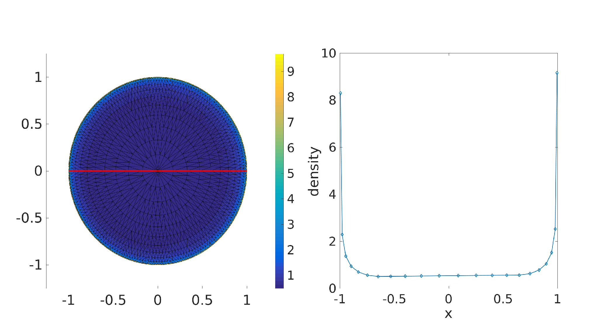
Refer to caption

Figure 3: Solution of the single layer equation at T=0.5T=0.5 along y=0y=0 on the circular screen, Example 1

Figure 4 examines the detailed singular behavior near the outer edge at (1,0)(1,0). It plots the numerical density at times T=0.5, 0.75, 1.0T=0.5,\ 0.75,\ 1.0 against the distance to the edge along xx-axis. In the log-log plot the slope of the curve near 00 corresponds to the edge exponent in decomposition (27).
The numerical solution exhibits edge singularities in close agreement with (27). Numerically, the singular exponents are within 8%8\% of the theoretical value of −12-\frac{1}{2} for the edge at these times. Note that the convergence of our boundary element method in the energy norm does not a priori imply convergence for the numerically computed singular exponents.

For Example 1, we finally consider the error compared to the benchmark solution on the 2-graded mesh. Because of the low spatial regularity of the solution, the numerical solutions cannot be expected to converge in L2​([0,T]×Γ)L^{2}([0,T]\times\Gamma). As a weaker measure, we consider the energy norm defined by the single layer operator, which is computed from the stiffness matrix VV and the solution vector uu as E⁡(ψ)=12​ψ⊤​V​ψ−ψ⊤​fE(\psi)=\frac{1}{2}\psi^{\top}V\psi-\psi^{\top}f. It is comparable or weaker than the norm of Hσ0​(ℝ+,H−12​(Γ))H^{0}_{\sigma}(\mathbb{R}^{+},{H}^{-\frac{1}{2}}(\Gamma)). For the error as a function of the degrees of freedom, Figure 5 shows convergence in the energy norm with a rate −0.52-0.52 on the 2-graded mesh, respectively −0.26-0.26 on the uniform mesh. The error therefore behaves in agreement with the approximation properties proportional to ∼h\sim h (equivalently, ∼D​O​F−12\sim DOF^{-\frac{1}{2}}) on the 2-graded mesh, while the convergence is ∼h1/2\sim h^{1/2} (∼DOF−1/4\sim DOF^{-1/4}) on a uniform mesh.

Refer to caption

Figure 4: Asymptotic behavior of the solution to the single layer equation near edge along y=0y=0, Example 1

Refer to caption

Figure 5: Energy error for single layer equation on circular screen, Example 1
Example 2.

Using the discretization from Section 3, we compute the solution to the integral equation V​ψ=fV\psi=f on ℝt+×Γ\mathbb{R}_{t}^{+}\times\Gamma with the square screen Γ=[−1,1]2×{0}\Gamma=[-1,1]^{2}\times\{0\} using the weak form (18), with constant test and ansatz functions in space and time. The right hand side is given by f(t,x)=cos(|k|t−k⋅x)exp(−1/(10t2))f(t,x)=\cos(|k|t-k\cdot x)\exp(-1/(10t^{2})), where k=(0.2,0.2,0.2)k=(0.2,0.2,0.2). The time discretization errors are negligibly small in this numerical experiment, when the time step is chosen to be Δ​t=0.005\Delta t=0.005. We compute the solution up to T=1T=1. The finest graded mesh consists of 23122312 triangles, and we use the solution on this mesh as reference solution using the same Δ​t=0.005\Delta t=0.005.

Figures 6 and 7 show the density along a cross-section and along a longitudinal section on a β\beta-graded mesh with β\beta=2 and 23122312 triangles at time T=0.5T=0.5. Both figures exhibit the corner and edge singularities predicted by the decomposition (31) and illustrate the qualitative behavior of the solution. Figure 8 compares the solution along the cross-section on a 22-graded mesh against the solution on two uniform meshes. We see that the 22-graded mesh yields a higher resolution of the corner singularities compared to the uniform meshes.

Refer to caption

Figure 6: Solution of the single layer equation at T=0.5T=0.5 along y=xy=x on the square screen, Example 2

Refer to caption

Figure 7: Solution of the single layer equation at T=0.5T=0.5 along y=0y=0 on the square screen, Example 2

Refer to caption

Figure 8: Numerical computation of the corner singularity along diagonal from (−1,−1)(-1,-1) to (1,1)(1,1) at time T=0.5T=0.5, Example 2

Figure 9 examines the detailed singular behavior near the corner (1,1)(1,1). It plots the numerical density at times T=0.5, 0.75, 1.0T=0.5,\ 0.75,\ 1.0 against the distance to the corner along the diagonal of the screen. In the log-log plot the slope of the curve near 00 corresponds to the corner exponent in decomposition (31). Similarly, Figure 10 shows the density as a function of xx for y=0y=0, perpendicular to the edge, at the same times.
After a short computational time, the numerical solution exhibits edge and corner singularities corresponding to (31). Numerically, the singular exponents at large enough times T=0.5, 0.75, 1T=0.5,\ 0.75,\ 1 are within 2%2\% of the theoretical value of −12-\frac{1}{2} for the edge, while they are around −0.78-0.78 for the corner, approximately 10%10\% higher than the theoretical exponent γ−1\gamma-1. Note that the convergence of our boundary element method in the energy norm does not a priori imply convergence for the numerically computed singular exponents.

Refer to caption

Figure 9: Asymptotic behavior of the solution to the single layer equation near corner along y=xy=x, Example 2

Refer to caption

Figure 10: Asymptotic behavior of the solution to the single layer equation near edge along y=0y=0, Example 2

Refer to caption

Figure 11: Energy error norm for single layer equation on square screen, Example 2

For Example 2, we finally consider the error compared to the benchmark solution on the 2-graded mesh. Like in Example 1, we consider the energy norm defined by the single layer operator. Figure 11 shows convergence of the norm with rates −0.54-0.54 on the 2-graded mesh, respectively −0.27-0.27 on the uniform mesh in terms of degrees of freedom. These closely mirror the approximation results, which predict an approximation error proportional to ∼h\sim h (equivalently, ∼D​O​F−12\sim DOF^{-\frac{1}{2}}) on the 2-graded mesh, while the approximation error is ∼h12\sim h^{\frac{1}{2}} (∼D​O​F−14\sim DOF^{-\frac{1}{4}}) on a uniform mesh. In particular, compared to Example 1, the corner singularities of the square screen do not affect the convergence rate.

To further probe the effect of the corners we also consider the L2L_{2} norm in time of the sound pressure evaluated in a point. For applications the approximation of the sound pressure away from the screen is often the most relevant measure. We evaluate the sound pressure by substituting the density ψΔ​t,h\psi_{\Delta t,h} into the single layer potential, pΔ​t,h=S​ψΔ​t,hp_{\Delta t,h}=S\psi_{\Delta t,h}, and use a tensor product Gaussian quadrature with 400400 nodes per triangle to evaluate the integral. Figure 12 shows the L2L_{2} error in time of the sound pressure evaluated in three points outside of the screen, (1,1,0.004)(1,1,0.004), (0.75,0.75,1)(0.75,0.75,1) and (1,1.25,0.25)(1,1.25,0.25). In each of the points, the convergence is proportional to ∼h2\sim h^{2}, resp. ∼h\sim h, as for the energy norm. However, while the convergence rate is in agreement with the energy norm, the error in the sound pressure strongly depends on the location of the point. In (1,1,0.004)(1,1,0.004), at distance 0.0040.004 from the corner of the screen, the error is an order of magnitude higher than in the points (0.75,0.75,1)(0.75,0.75,1) and (1,1.25,0.25)(1,1.25,0.25), which are at a distance of order 11.

Refer to caption

Figure 12: L2​([0,T])L_{2}([0,T]) error for the sound pressure in three points outside square screen, computed from single layer equation, Example 2

6.2 Hypersingular operator

Example 3.

Using the discretization from Section 3, we compute the solution to the integral equation W​ϕ=gW\phi=g on ℝt+×Γ\mathbb{R}_{t}^{+}\times\Gamma with the circular screen Γ={(x,y,0):0≤x2+y2≤1}\Gamma=\{(x,y,0):0\leq\sqrt{x^{2}+y^{2}}\leq 1\} depicted in Figure 1. We use the weak form (19) with linear ansatz and test functions in space, linear ansatz and constant test functions in time. Here,

g⁡(t,x)\displaystyle g{(t,x)} =(−34+cos⁡(π2​(4−t))+π2​sin⁡(π2​(4−t))−14​(cos⁡(π⁡(4−t))+π​sin⁡(π⁡(4−t))))\displaystyle=\textstyle{(-\frac{3}{4}+\cos(\frac{\pi}{2}(4-t))+\frac{\pi}{2}\sin(\frac{\pi}{2}(4-t))-\frac{1}{4}(\cos({\pi}(4-t))+\pi\sin({\pi}(4-t))))}
×[H⁡(4−t)−H⁡(−t)],\displaystyle\qquad\times[H(4-t)-H(-t)],

where HH is the Heaviside function. The time discretization errors are negligibly small in this numerical experiment, when the time step is chosen to be Δ​t=0.01\Delta t=0.01. We compute the solution up to T=4T=4. The finest graded mesh consists of 2662 triangles, and we use the solution on this mesh as reference solution using the same Δ​t=0.01\Delta t=0.01.

Refer to caption

Figure 13: Solution of the hypersingular equation at T=2T=2 along y=0y=0 on the circular screen, Example 3

Figure 13 shows the density along a cross-section on a β\beta-graded mesh with β\beta=2 and 2662 triangles at time T=2T=2. The figure exhibits the edge singularities predicted by the decomposition (26) and illustrates the qualitative behavior of the solution.

Refer to caption

Figure 14: Asymptotic behavior of the solution to the hypersingular equation near edge along y=0y=0, Example 3

Figure 14 examines the detailed singular behavior at the circular edge along the xx-axis near the point (1,0)(1,0). It plots the numerical density at times up to T=2.5T=2.5 against the distance to the edge. For the singular exponents, we numerically obtain values within 5%5\% of the theoretical value of 12\frac{1}{2}, except at the earliest time T=0.5T=0.5, when compute an exponent 0.410.41.

Refer to caption

Figure 15: L2​([0,T],L2​(Γ))L_{2}([0,T],L_{2}(\Gamma)) and energy error for hypersingular equation on circular screen, Example 3

Finally, Figure 15 shows the error in both the energy and L2​([0,T],L2​(Γ))L_{2}([0,T],L_{2}(\Gamma)) norms with respect to the benchmark solution. The convergence rate in terms of the degrees of freedom on the 22-graded mesh is −0.47-0.47 in energy and −0.93-0.93 in L2L_{2}. It is in close agreement with a convergence proportional to ∼h\sim h (equivalently, ∼DOF−1/2\sim DOF^{-1/2}) predicted by the approximation properties in the energy norm, and ∼h2\sim h^{2} (equivalently, ∼D​O​F−1\sim DOF^{-1}) in L2L_{2}. On the uniform mesh the rate is −0.18-0.18 in energy and −0.33-0.33 in L2L_{2}.

Example 4.

Using the discretization from Section 3, with test and ansatz functions as in Example 3, we compute the solution to the integral equation W​ϕ=gW\phi=g on ℝt+×Γ\mathbb{R}_{t}^{+}\times\Gamma with the square screen Γ=[−1,1]2×{0}\Gamma=[-1,1]^{2}\times\{0\}. We prescribe the right hand side

g⁡(t,x)\displaystyle g{(t,x)} =(−34+cos⁡(π2​(4−t))+π2​sin⁡(π2​(4−t))−14​(cos⁡(π⁡(4−t))+π​sin⁡(π⁡(4−t))))\displaystyle=(-\frac{3}{4}+\cos(\frac{\pi}{2}(4-t))+\frac{\pi}{2}\sin(\frac{\pi}{2}(4-t))-\frac{1}{4}(\cos({\pi}(4-t))+\pi\sin({\pi}(4-t))))
×[H⁡(4−t)−H⁡(−t)],\displaystyle\qquad\times[H(4-t)-H(-t)],

where HH is the Heaviside function, and set Δ​t=0.01\Delta t=0.01, T=4T=4. The finest graded mesh consists of 23122312 triangles, and we use the solution on this mesh as reference solution using the same Δ​t=0.01\Delta t=0.01.

The density along the diagonal x=yx=y, respectively along y=0y=0, exhibit the corner and edge singularities predicted by the decomposition (30). The qualitative behavior of the solution at T=2T=2 along the diagonal y=xy=x of the square screen is shown in Figure 16, illustrating the singularity in the corners. Figure 17 shows the behaviour along y=0y=0, with the edge singularity at the boundary of the screen. As the solution to the hypersingular equation lies in Hσ12​(ℝ+,H~12​(Γ)){H}^{\frac{1}{2}}_{\sigma}(\R^{+},\tilde{H}^{\frac{1}{2}}(\Gamma)), its conforming numerical approximation tends to zero at both edges and corners.

Refer to caption

Figure 16: Solution of the hypersingular equation at T=2T=2 along y=xy=x on the square screen, Example 4

Refer to caption

Figure 17: Solution of the hypersingular equation at T=2T=2 along y=0y=0 on the square screen, Example 4

Figure 18 examines the detailed singular behavior near the corner (1,1)(1,1). It plots the numerical density at times up to T=2.5T=2.5 against the distance to the corner along the diagonal of the screen. The numerically computed singular exponents in the corner of around 0.670.67 do not show good agreement with the exact corner exponent γ\gamma. The density as a function of xx for y=0y=0, perpendicular to the edge, is shown in Figure 19 at the same times. Unlike for the corner exponent, the numerically computed singular exponent at the edge, around 0.480.48, is witin 8%8\% of the exact value 12\frac{1}{2} for early times, and within 4%4\% for T≥1.5T\geq 1.5.

Refer to caption

Figure 18: Asymptotic behavior of the solution to the hypersingular equation near corner along y=xy=x, Example 3

Refer to caption

Figure 19: Asymptotic behavior of the solution to the hypersingular equation near edge along y=0y=0, Example 3

Refer to caption

Figure 20: L2​([0,T],L2​(Γ))L_{2}([0,T],L_{2}(\Gamma)) and energy error for hypersingular equation on square screen, Example 4

Finally, Figure 20 shows the error in both the energy and L2​([0,T],L2​(Γ))L_{2}([0,T],L_{2}(\Gamma)) norms with respect to the benchmark solution. The convergence rate in terms of the degrees of freedom on the 22-graded mesh is −0.51-0.51 in energy and −1.05-1.05 in L2L_{2}. On the uniform mesh the rate is −0.26-0.26 in energy and −0.50-0.50 in L2L_{2}. The rates on the 22-graded meshes are in close agreement with a convergence proportional to ∼h\sim h (equivalently, ∼DOF−1/2\sim DOF^{-1/2}) predicted by the approximation properties in the energy norm, and ∼h1/2\sim h^{1/2} (∼DOF−1/4\sim DOF^{-1/4}) on uniform meshes. Also in L2L_{2} norm, the convergence corresponds to the expected rates: Approximately ∼h2\sim h^{2} (equivalently, ∼D​O​F−1\sim DOF^{-1}) on 22-graded meshes, ∼h\sim h (equivalently, ∼DOF−1/2\sim DOF^{-1/2}) on uniform meshes. In all cases the convergence is twice as fast on the 22-graded compared to the uniform meshes.

6.3 Dirichlet-to-Neumann operator

In addition to the single layer and hypersingular operators in the previous subsections, we also consider the Dirichlet-to-Neumann operator on the screen. Compared to the hypersingular operator, the Dirichlet-to-Neumann operator is not available in closed form and requires approximation. It is of interest to see the influence of the approximation of the operator on the numerical solution.

Example 5.

Using the discretization from Section 3, we compute the solution to the integral equation 𝒮​u=h\mathcal{S}u=h on ℝt+×Γ\mathbb{R}_{t}^{+}\times\Gamma with Γ=[−1,1]2×{0}\Gamma=[-1,1]^{2}\times\{0\}. We prescribe the right hand side

h⁡(t,x)\displaystyle h{(t,x)} =(−34+cos⁡(π2​(4−t))+π2​sin⁡(π2​(4−t))−14​(cos⁡(π⁡(4−t))+π​sin⁡(π⁡(4−t))))\displaystyle=\textstyle{(-\frac{3}{4}+\cos(\frac{\pi}{2}(4-t))+\frac{\pi}{2}\sin(\frac{\pi}{2}(4-t))-\frac{1}{4}(\cos({\pi}(4-t))+\pi\sin({\pi}(4-t))))}
×[H⁡(4−t)−H⁡(−t)],\displaystyle\qquad\times[H(4-t)-H(-t)],

where HH is the Heaviside function, and set Δ​t=0.01\Delta t=0.01, T=0.65T=0.65. The finest graded mesh consists of 23122312 triangles, and we use the solution on this mesh as reference solution using the same Δ​t=0.01\Delta t=0.01.

Figures 21 and 22 show the density along a cross-section and along a longitudinal section on a β\beta-graded mesh with β\beta=2 and 23122312 triangles at time T=0.5T=0.5. Both figures exhibit the corner and edge singularities predicted by the decomposition 30 and illustrate the qualitative behavior of the solution. As the solution to the Dirichlet-to-Neumann equation lies in Hσ12​(ℝ+,H~12​(Γ)){H}^{\frac{1}{2}}_{\sigma}(\R^{+},\tilde{H}^{\frac{1}{2}}(\Gamma)), its conforming numerical approximation is zero at the boundary of the screen.

Figure 23 examines the detailed singular behavior near the corner (1,1)(1,1). It plots the numerical density at times T=0.25, 0.5, 0.6, 0.65T=0.25,\ 0.5,\ 0.6,\ 0.65 against the distance to the corner along the diagonal of the screen. In the log-log plot the slope of the curve near 00 corresponds to the corner exponent in the singular expansion. Similarly, Figure 24 shows the density as a function of yy for x=−0.8754x=-0.8754, perpendicular to the edge, at the same times. The numerically computed singular exponents of the edge, around 0.40.4, are in qualitative agreement with the exact value 12\frac{1}{2}. For the corner, the computed value above 0.60.6 differs significantly from the exact value γ\gamma. A similar difference was observed in the previous section for the hypersingular operator, so that the approximation involved in computing the Dirichlet-to-Neumann operator is not the source of this discrepancy.

Refer to caption

Figure 21: Solution of the Dirichlet-to-Neumann equation at T=0.65T=0.65 along y=xy=x on the square screen, Example 5

Refer to caption

Figure 22: Solution of the Dirichlet-to-Neumann equation at T=0.65T=0.65 along x=−0.8754x=-0.8754 on the square screen, Example 5

Refer to caption

Figure 23: Asymptotic behavior of the solution to the Dirichlet-to-Neumann equation near corner along y=xy=x, Example 5

Refer to caption

Figure 24: Asymptotic behavior of the solution to the Dirichlet-to-Neumann equation near edge along x=−0.8754x=-0.8754, Example 5

Refer to caption

Figure 25: Error in L2​([0,T],L2​(Γ))L_{2}([0,T],L_{2}(\Gamma)) norm for Dirichlet-to-Neumann equation on square screen, Example 5

Figure 25 shows the error in L2​([0,T]×Γ)L^{2}([0,T]\times\Gamma) compared to the benchmark solution. The convergence in this norm is proportional to ∼h2\sim h^{2} (equivalently, ∼D​O​F−1\sim DOF^{-1}) on the 2-graded mesh, while the convergence is ∼h1\sim h^{1} (∼D​O​F−12\sim DOF^{-\frac{1}{2}}) on a uniform mesh. This coincides with the rates expected from the approximation property of the graded, respectively uniform meshes, and it is also in agreement with the rates obtained for the hypersingular operator on the square screen in the previous section.

7 Applications to traffic noise: Horn effect

For applications in traffic noise, the natural (simplified) geometry is that of a half-space ℝ+3\mathbb{R}^{3}_{+} with a tire, as displayed in Figure 26. The horn like geometry between the tire and the street amplifies sound sources close to the contact patch, and it is of interest to compute the amplification for a broad band of frequencies. See also [5, 27]. See [21, 22] for the complementary problem of the tire dynamics in contact with the road.

We consider the wave equation for the sound pressure scattered by the tire, with homogeneous Neumann conditions on the street Γ∞=ℝ2×{0}\Gamma_{\infty}=\mathbb{R}^{2}\times\{0\} and inhomogeneous Neumann conditions on the tire. Note that the boundary conditions jump in the cuspidal geometry between the tire and the road surface. The relevant Green’s function in ℝ+3\mathbb{R}^{3}_{+} is given by

G⁡(t,x,y)=δ⁡(t−|x−y|)4​π​|x−y|+δ⁡(t−|x−y′|)4​π​|x−y′|,\displaystyle G(t,x,y)=\frac{\delta(t-|x-y|)}{4\pi|x-y|}+\frac{\delta(t-|x-y^{\prime}|)}{4\pi|x-y^{\prime}|}\ , (37)

where y′y^{\prime} is the reflection of yy on Γ∞\Gamma_{\infty}. We use it in a single layer potential ansatz for a sound pressure scattered by the tire,

p⁡(t,x)=14​π​∫Γϕ⁡(t−|x−y|,y)|x−y|​d​sy+14​π​∫Γϕ⁡(t−|x−y′|,y)|x−y′|​d​sy,\displaystyle p(t,x)=\frac{1}{4\pi}\int_{\Gamma}\frac{\phi(t-|x-y|,y)}{|x-y|}\,ds_{y}+\frac{1}{4\pi}\int_{\Gamma}\frac{\phi(t-|x-y^{\prime}|,y)}{|x-y^{\prime}|}\,ds_{y}\ , (38)

with ϕ⁡(s,y)=0\phi(s,y)=0 for s≤0s\leq 0. The Neumann problem for the scattered sound translates into an integral equation for ϕ\phi:

(−I+K′)​ϕ​(t,x)=2​∂p∂n​(t,x)=−2​∂pI∂n​(t,x),\displaystyle\left(-I+K^{\prime}\right)\phi(t,x)=2\frac{\partial p}{\partial n}(t,x)=-2\frac{\partial p^{I}}{\partial n}(t,x)\ , (39)

with pIp^{I} the incoming wave and the adjoint double layer operator K′K^{\prime} from (4),

K′​ϕ​(t,x)=\displaystyle K^{\prime}\phi(t,x)= 12​π​∫Γnx⊤​(y−x)|x−y|​(ϕ⁡(t−|x−y|,y)|x−y|2+ϕ˙​(t−|x−y|,y)|x−y|)​d​sy\displaystyle\frac{1}{2\pi}\int_{\Gamma}\frac{n_{x}^{\top}(y-x)}{|x-y|}\left(\frac{\phi(t-|x-y|,y)}{|x-y|^{2}}+\frac{\dot{\phi}(t-|x-y|,y)}{|x-y|}\right)\,ds_{y}
+12​π∫Γnx⊤​(y′−x)|x−y′|(ϕ⁡(t−|x−y′|,y)|x−y′|2+ϕ˙​(t−|x−y′|,y)|x−y′|)dsy.\displaystyle+\frac{1}{2\pi}\int_{\Gamma}\frac{n_{x}^{\top}(y^{\prime}-x)}{|x-y^{\prime}|}\left(\frac{\phi(t-|x-y^{\prime}|,y)}{|x-y^{\prime}|^{2}}+\frac{\dot{\phi}(t-|x-y^{\prime}|,y)}{|x-y^{\prime}|}\right)\,ds_{y}.

The weak formulation reads:
Find ϕ∈Hσ12​(ℝ+,H~−12​(Γ))\phi\in H^{\frac{1}{2}}_{\sigma}(\mathbb{R}^{+},\widetilde{H}^{-\frac{1}{2}}(\Gamma)) such that for all test functions ψ∈Hσ12​(ℝ+,H−12​(Γ))\psi\in H^{\frac{1}{2}}_{\sigma}(\mathbb{R}^{+},H^{-\frac{1}{2}}(\Gamma))

∫0∞∫Γ(−I+K′)ϕψdsxdσt=−2∫0∞∫Γ∂pI∂nψdsxdσt.\displaystyle\int_{0}^{\infty}\int_{\Gamma}\left(-I+K^{\prime}\right)\phi\ \psi\ \,ds_{x}\,d_{\sigma}t=-2\int_{0}^{\infty}\int_{\Gamma}\frac{\partial p^{I}}{\partial n}\ \psi\,ds_{x}\,d_{\sigma}t\ . (40)

It is discretized with piecewise constant ansatz and test functions ψih​(x)​γΔ​tn​(t)∈Vt,h0,0\psi_{i}^{h}(x)\gamma^{n}_{\Delta t}(t)\in V^{0,0}_{t,h} in space and time.

To obtain the sound amplification for the entire frequency spectrum in one time domain computation, we consider the sound emitted by a Dirac point source. It is located in the point ys​r​c=(0.08,0,0)y_{src}=(0.08,0,0) near the horn,

pI=δ⁡(t−|x−ys​r​c|)4​π​|x−ys​r​c|+δ⁡(t−|x−ys​r​c′|)4​π​|x−ys​r​c′|.\displaystyle p^{I}=\frac{\delta(t-|x-y_{src}|)}{4\pi|x-y_{src}|}+\frac{\delta(t-|x-y^{\prime}_{src}|)}{4\pi|x-y^{\prime}_{src}|}\ . (41)

The right hand side of the discretization of the integral equation (40) is calculated to be [5]

−2∫0∞∫Γ∂pI∂nψihγΔ​tndsxdt=−∫Ti∩E⁡(ys​r​c)nx⊤​(ys​r​c−x)π|x−ys​r​c|3dsx+nx⊤(ys​r​c−x){ζ⁡(tn−1)π​tn−12−ζ⁡(tn)π​tn2}.\displaystyle-2\int_{0}^{\infty}\int_{\Gamma}\frac{\partial p^{I}}{\partial n}\psi_{i}^{h}\gamma^{n}_{\Delta t}\,ds_{x}\,dt=-\int_{T_{i}\cap E(y_{src})}\frac{n_{x}^{\top}(y_{src}-x)}{\pi\arrowvert x-y_{src}\arrowvert^{3}}\,ds_{x}+n_{x}^{\top}(y_{src}-x)\left\{\frac{\zeta(t_{n-1})}{\pi t_{n-1}^{2}}-\frac{\zeta(t_{n})}{\pi t_{n}^{2}}\right\}\ .

The first term is an integral over the domain of influence E⁡(ys​r​c)={x∈Γ:tn−1≤|x−ys​r​c|≤tn}E(y_{src}){=\{x\in\Gamma:t_{n-1}\leq|x-y_{src}|\leq t_{n}\}} of ys​r​cy_{src}, intersected with Ti=supp​ψihT_{i}=\mathrm{supp}\ \psi_{i}^{h}, and it is computed in the same way as the entries of the Galerkin matrix. In the second term, ζ⁡(t)\zeta(t) denotes the length of the curve segment Ti∩{|x−ys​r​c|=t}T_{i}\cap\{\arrowvert x-y_{src}\arrowvert=t\} inside the triangle TiT_{i}.

Refer to caption
Figure 26: Cross section of geometrical setup for horn effect.

After solving the discretization of (40) for the density ϕ\phi, we obtain the sound pressure pp in the receiver point xf​p=(1,0,0)x_{fp}=(1,0,0) from (38). From [27, Eq. 7], the amplification factor is given by:

Δ​LH​(ω)=20​log10⁡(|p^​(ω,xf​p)+p^I​(ω,xf​p)||p^I​(ω,xf​p)|).\Delta L_{H}(\omega)=20\log_{10}\left(\frac{|\hat{p}(\omega,x_{fp})+\hat{p}^{I}(\omega,x_{fp})|}{|\hat{p}^{I}(\omega,x_{fp})|}\right)\ .

Here, p^\hat{p} and p^I\hat{p}^{I} denote the Fourier transformed incident and scattered sound pressure fields. The Fourier transformation is calculated using a discrete FFT, where the time step size is the same as for the computation of the density.

In the geometry given by Figure 26, we compute the sound amplification in standard units for a grown slick 205/55R16 tire at 2 bar pressure. It is subject to 3415N axle load at 50 km/h on a street with an ISO 10844 surface, and a mesh with 6027 nodes is depicted in Figure 27. We use this and a refined graded mesh and consider the sound amplification for frequencies between 200200 and 20002000 Hz. The total time interval is T=24T=24 and the time step sizes Δ​t=0.005, 0.01, 0.04\Delta t=0.005,\ 0.01,\ 0.04. For smaller time step sizes more reflections in the horn can be resolved, and these are responsible for the sound amplification.

We compare the results for the uniform mesh with a refined, graded-like mesh with grading parameter β=2\beta=2, see Figure 27. Figure 28 shows approximations of the amplification factor in the horn geometry, discretized using the graded mesh, across the frequency range for the time step sizes Δ​t=0.005, 0.01, 0.04\Delta t=0.005,\ 0.01,\ 0.04. We also show the approximation given by the uniform tire mesh for Δ​t=0.005\Delta t=0.005. The figure, in particular, exhibits several resonances between 10001000 and 20002000 Hz, at which the different approximations lead to significant differences in the computed amplification factors.

The differences between the computed amplification factors are depicted in Figure 29. The first subfigure considers the differences between the graded and uniform meshes for a given time step size, Δ​t=0.005, 0.01, 0.04\Delta t=0.005,\ 0.01,\ 0.04. Outside the resonance frequencies the differences are negligible. Especially in the strong resonances around 13001300 and 19001900 Hz, however, the difference between graded and uniform meshes becomes more and more relevant for smaller Δ​t\Delta t, as the small time step allows to resolve the reflections in the horn geometry more accurately. The second subfigure of Figure 29 compares the computed amplification for graded meshes for different Δ​t\Delta t. As before, the differences are mostly relevant near resonance frequencies, and the discretization error for a fixed mesh decreases with Δ​t\Delta t. For Δ​t=0.005\Delta t=0.005 the differences between the spatial, resp. temporal discretizations in Figure 29 are both around 66 dB near 13001300 Hz. Such differences in sound pressure are significant to the human perception. They indicate the relevance of graded meshes for computations of traffic noise.

Refer to caption
Refer to caption
Figure 27: Mesh of (a) slick 205/55R16 tire and (b) graded refinement.
Refer to caption
Figure 28: Amplification due to horn effect: Graded mesh approximations for different Δ​t\Delta t, compared to a uniform mesh approximation.
Refer to caption
Refer to caption
Figure 29: Differences of amplification factors in d​BdB between graded and uniform meshes for fixed Δ​t\Delta t, resp. between graded meshes for different Δ​t\Delta t.

Acknowledgement

We thank one of the referees for particularly helpful suggestions which improved the article.

References

  • [1] I. Babuška, Finite element method for domains with corners, Computing 6 (1970), 264-273.
  • [2] I. Babuška, R. B. Kellogg, J. Pitkäranta, Direct and inverse error estimates for finite elements with mesh refinements, Numer. Math. 33 (1979), 447-471.
  • [3] A. Bamberger, T. Ha Duong, Formulation variationnelle espace-temps pour le calcul par potentiel retarde d’une onde acoustique, Math. Meth. Appl. Sci. 8 (1986), 405-435 and 598-608.
  • [4] L. Banjai, Time-domain Dirichlet-to-Neumann map and its discretization, IMA J. Numer. Anal. 34 (2014), 1136-1155.
  • [5] L. Banz, H. Gimperlein, Z. Nezhi, E. P. Stephan, Time domain BEM for sound radiation of tires, Computational Mechanics 58 (2016), 45-57.
  • [6] E. Becache, T. Ha-Duong, A space-time variational formulation for the boundary integral equation in a 2d elastic crack problem, RAIRO 28 (1994), 141-176.
  • [7] M. Costabel, Time-dependent problems with the boundary integral equation method, Encyclopedia of Computational Mechanics (2004), 1-25.
  • [8] M. Dauge, Elliptic boundary value problems in corner domains, Lecture Notes in Mathematics 1341, Springer-Verlag, 1988.
  • [9] V. Ervin, E. P. Stephan, A boundary-element method with mesh refinement for a weakly singular integral equation, Communications in Applied Numerical Methods 7 (1991), 273-280.
  • [10] V. Ervin, E. P. Stephan, An improved boundary element method for the charge density of a thin electrified plate in ℝ3\mathbb{R}^{3}, Mathematical Methods in the Applied Sciences 13 (1990), 291-303.
  • [11] H. Gimperlein, M. Maischak, E. P. Stephan, Adaptive time domain boundary element methods and engineering applications, Journal of Integral Equations and Applications 29 (2017), 75-105.
  • [12] H. Gimperlein, F. Meyer, C. Oezdemir, E. P. Stephan, Time domain boundary elements for dynamic contact problems, Computer Methods in Applied Mechanics and Engineering (2018), to appear.
  • [13] H. Gimperlein, Z. Nezhi, E. P. Stephan, A priori error estimates for a time-dependent boundary element method for the acoustic wave equation in a half-space, Mathematical Methods in the Applied Sciences 40 (2017), 448-462.
  • [14] H. Gimperlein, C. Oezdemir, D. Stark, E. P. Stephan, A residual a posteriori estimate for the time-domain boundary element method, preprint.
  • [15] H. Gimperlein, C. Özdemir, E. P. Stephan, Time domain boundary element methods for the Neumann problem: Error estimates and acoustic problems, Journal of Computational Mathematics 36 (2018), 70-89.
  • [16] M. Gläfke, Adaptive Methods for Time Domain Boundary Integral Equations, Ph.D. thesis, Brunel University London (2012).
  • [17] J. Gwinner, E. P. Stephan, Advanced Boundary Element Methods – Treatment of Boundary Value, Transmission and Contact Problems, draft of book (2017).
  • [18] T. Ha-Duong, Equations integrales pour la resolution numerique de preblemes de diffraction d’ondes acoustiques dans ℝ3\R^{3}, Ph.D. thesis, Université Pierre et Marie Curie Paris (1987).
  • [19] T. Ha-Duong, On retarded potential boundary integral equations and their discretizations, Topics in computational wave propagation, Lect. Notes Comput. Sci. Eng. 31 (2003), 301-336.
  • [20] T. Ha-Duong, On the transient acoustic scattering by a flat object, Japan J. Appl. Math. 7 (1990), 489-513.
  • [21] C. Hager, P. Hauret, P. Le Tallec, B. I. Wohlmuth, Solving dynamic contact problems with local refinement in space and time, Comput. Methods Appl. Mech. Engrg. 201/204 (2012), 25–41.
  • [22] P. Hauret, J. Salomon, A. A. Weiss, B. I. Wohlmuth, Energy-consistent corotational schemes for frictional contact problems, SIAM J. Sci. Comput. 30 (2008), 2488–2511.
  • [23] H. Holm, M. Maischak, E. P. Stephan, The hp-version of the boundary element method for Helmholtz screen problems, Computing 57 (1996), 105-134.
  • [24] A. Y. Kokotov, P. Neittaanmäki, B. A. Plamenevskiǐ, The Neumann problem for the wave equation in a cone, J. Math. Sci. 102 (2000), 4400-4428.
  • [25] A. Y. Kokotov, P. Neittaanmäki, B. A. Plamenevskiǐ, Diffraction on a cone: The asymptotics of solutions near the vertex, J. Math. Sci. 109 (2002), 1894-1910.
  • [26] A. Y. Kokotov, P. Neittaanmäki, B. A. Plamenevskiǐ, On the asymptotic behavior of solutions of the Neumann problem for hyperbolic systems in domains with conical points, Algebra i Analiz 16 (2004), 56-98.
  • [27] W. Kropp, F. X. Becot, S. Barrelet, On the sound radiation from tyres, Acta Acustica united with Acustica 86 (2000), 769-779.
  • [28] M. Maischak, E. P. Stephan, The h-p-version of the BEM with geometric meshes in 3D, Boundary Element Topics (1997), 351-362.
  • [29] M. Maischak, Manual of the software package maiprogs, Version 3.7.1 ed., August, 2012.
  • [30] S. I. Matyukevich, B. A. Plamenevskiǐ, On dynamic problems in the theory of elasticity in domains with edges, Algebra i Analiz 18 (2006), 158-233.
  • [31] V. G. Maz’ya, J. Rossmann, Elliptic equations in polyhedral domains, Mathematical Surveys and Monographs, Vol. 162, American Mathematical Society, Providence, RI, 2010.
  • [32] F. Müller, C. Schwab, Finite Elements with mesh refinement for wave equations in polygons, J. Comp. Appl. Math. 283 (2015), 163-181.
  • [33] B. A. Plamenevskiǐ, On the Dirichlet problem for the wave equation in a cylinder with edges, Algebra i Analiz 10 (1998), 197-228.
  • [34] S. Sauter, C. Schwab, Boundary Element Methods, Springer Series in Computational Mathematics 39 (2011).
  • [35] J. F. Sayas, Retarded Potentials and Time Domain Boundary Integral Equations: A Road Map, Springer Series in Computational Mathematics 50 (2016).
  • [36] T. von Petersdorff, Randwertprobleme der Elastizitätstheorie für Polyeder-Singularitäten und Approximation mit Randelementmethoden, Ph.D. thesis, Technische Universität Darmstadt (1989).
  • [37] T. von Petersdorff, E. P. Stephan, Regularity of mixed boundary value problems in ℝ3\mathbb{R}^{3} and boundary element methods on graded meshes, Math. Methods Appl. Sci. 12 (1990), 229-249.
  • [38] T. von Petersdorff, E. P. Stephan, Decompositions in edge and corner singularities for the solution of the Dirichlet problem of the Laplacian in a polyhedron, Math. Nachr. 149 (1990), 71-103.
  • [39] T. von Petersdorff, E. P. Stephan, Singularities of the solution of the Laplacian in domains with circular edges, Appl. Analysis 45 (1992), 281-294.
  • [40] B. Sako, A Model for the Crack and Punch Problems in Elasticity, Ph.D. thesis, University of California, Los Angeles (1986).
  • [41] A. Veit, Numerical methods for time-domain boundary integral equations, Ph.D. thesis, Universität Zürich (2012).