Strong cosmic censorship in de Sitter space

We will write the Kerr-de Sitter metric [22] as follows [23]

$$ds^{2}=\rho^{2}\left[\frac{\mathrm{d}r^{2}}{\Delta_{r}}+\frac{\mathrm{d}\chi^{2}}{\Delta_{\chi}}\right]+\frac{1}{\rho^{2}\Xi^{2}}\left[\Delta_{\chi}\left(\mathrm{d}t-\frac{\sigma_{r}}{a}\mathrm{d}\phi\right)^{2}-\Delta_{r}\left(\mathrm{d}t-\frac{\sigma_{\chi}}{a}\mathrm{d}\phi\right)^{2}\right]$$

(3.4)

where

$$\sigma_{r}=a^{2}+r^{2}\,,\qquad\sigma_{\chi}=a^{2}-\chi^{2}\,,\qquad\rho^{2}=r^{2}+\chi^{2}\,,\qquad\Xi=1+\frac{a^{2}}{L^{2}}$$

(3.5)

and

$$\Delta_{r}=\sigma_{r}\left(1-\frac{r^{2}}{L^{2}}\right)-2\,M\,r\,,\qquad\Delta_{\chi}=\sigma_{\chi}\left(1+\frac{\chi^{2}}{L^{2}}\right)\,,\qquad\Lambda=\frac{3}{L^{2}}\,.$$

(3.6)

In these coordinates, $\phi\in[0,2\pi)$ and $\chi\in[-|a|,|a|]$. It is convenient to define

$$\Omega(r)=\frac{a}{r^{2}+a^{2}}\,.$$

(3.7)

We assume that the solution describes a non-extremal black hole, which implies that there are three real positive roots of $\Delta_{r}$, satisfying $r_{-}<r_{+}<r_{c}$. These correspond to the Cauchy horizon, event horizon and cosmological horizon, respectively. The angular velocities of the horizons will be denoted by

$$\Omega_{-}=\Omega(r_{-}),\qquad\Omega_{+}=\Omega(r_{+}),\qquad\Omega_{c}=\Omega(r_{c}).$$

(3.8)

Starting from the above metric with $r_{+}<r<r_{c}$, which we call region I (see Fig. 1), we define ingoing coordinates $(v,r,\chi,\phi^{\prime})$ as follows:

$$\mathrm{d}t=\mathrm{d}v-\frac{\Xi\,\sigma_{r}}{\Delta_{r}}\mathrm{d}r\qquad\mathrm{d}\phi=\mathrm{d}\phi^{\prime}-\frac{a\,\Xi}{\Delta_{r}}\mathrm{d}r\,.$$

(3.9)

In the ingoing coordinates, we can extend across $r=r_{+}$ into a new region, region II (see Fig. 1), with $r_{-}<r<r_{+}$. In the new coordinates $g_{rr}=0$ so $\partial/\partial r$ is globally null. In fact $\partial/\partial r$ is also geodesic and shear free: it is one of the repeated principal null directions of the solution; $-\partial/\partial r$ is tangent to ingoing null geodesics.

In region II we can re-introduce the original coordinates $(t,r,\chi,\phi)$ using (3.9). The metric in these coordinates takes the same form as (3.4). Now, in region II, we introduce outgoing coordinates $(u,r,\chi,\phi^{\prime\prime})$ defined by

$$\mathrm{d}t=\mathrm{d}u+\frac{\Xi\,\sigma_{r}}{\Delta_{r}}\mathrm{d}r\qquad\mathrm{d}\phi=\mathrm{d}\phi^{\prime\prime}+\frac{a\,\Xi}{\Delta_{r}}\mathrm{d}r\,.$$

(3.10)

This lets us analytically continue the metric across the “right” Cauchy horizon $\mathcal{CH}_{R}^{+}$ in region II into a new region with $r<r_{-}$. In these coordinates, $-\partial/\partial r$ is null, geodesic and shear free, and future-directed. It is the second repeated principal null direction of the solution. It is tangent to outgoing null geodesics in region II, i.e., null geodesics which cross ${\cal CH}_{R}^{+}$.

We will parametrise Kerr-de Sitter solutions using the dimensionless quantities

$$\{y_{+},\alpha\}\equiv\{r_{+}/r_{c},a/r_{c}\}$$

(3.11)

These variables are in one-to-one correspondence with members of the Kerr-de Sitter family of solutions and mean we essentially normalise all our quantities to $r_{c}$. The moduli space of solutions is shown in Fig. 2. Kerr-de Sitter black holes have three distinct extremal limits: $r_{+}=r_{-}$, $r_{+}=r_{c}$ and $r_{+}=r_{-}=r_{c}$. The first two are marked as the black dashed line and red dotted-dashed line in Fig. 2, respectively. For completeness, we also show in Fig. 2 the Schwarzschild limit marked as a green solid line.

When $r_{+}=r_{-}$, we have

$$|a|=|a_{\mathrm{ext}}|\equiv\frac{r_{c}}{\sqrt{2}}\sqrt{(1+y_{+})\sqrt{1+2y_{+}+9y_{+}^{2}}-y_{+}(2+3y_{+})-1}\,.$$

(3.12)

When we study gravitational perturbations of Kerr-de Sitter black holes, it will be useful to introduce a null tetrad $\{\bm{\ell},\bm{n},\bm{m},\bar{\bm{m}}\}$ satisfying the following orthogonality relations

$$\bm{\ell}\cdot\bm{n}=-1\,,\quad\bar{\bm{m}}\cdot\bm{m}=1$$

(3.13)

with all remaining combinations of inner products giving zero, and $g_{\mu\nu}=-2\bm{\ell}_{(\mu}\bm{n}_{\nu)}+2\bm{m}_{(\mu}\bm{\overline{m}}_{\nu)}$.

There is obviously a lot of freedom in choosing such tetrad, and some choices make the equations governing gravitational perturbations of Kerr-de Sitter black holes easier than others. Here we will choose the Chambers-Moss null tetrad $\{\bm{\ell},\bm{n},\bm{m},\bm{\overline{m}}\}$ [23], which in $\{t,r,\chi,\phi\}$ coordinates, reads:

	$\displaystyle\bm{\ell}^{\mu}\partial_{\mu}=\frac{1}{\sqrt{2}\sqrt{r^{2}+\chi^{2}}}\left(\Xi\,\frac{a^{2}+r^{2}}{\sqrt{\Delta_{r}}}\,\partial_{t}+\sqrt{\Delta_{r}}\,\partial_{r}+\frac{a\,\Xi}{\sqrt{\Delta_{r}}}\,\partial_{\phi}\right),$
	$\displaystyle\bm{n}^{\mu}\partial_{\mu}=\frac{1}{\sqrt{2}\sqrt{r^{2}+\chi^{2}}}\left(\Xi\,\frac{a^{2}+r^{2}}{\sqrt{\Delta_{r}}}\,\partial_{t}-\sqrt{\Delta_{r}}\,\partial_{r}+\frac{a\,\Xi}{\sqrt{\Delta_{r}}}\,\partial_{\phi}\right),$
	$\displaystyle\bm{m}^{\mu}\partial_{\mu}=-\frac{i}{\sqrt{2}\sqrt{r^{2}+\chi^{2}}}\left(\Xi\,\frac{a^{2}-\chi^{2}}{\sqrt{\Delta_{\chi}}}\,\partial_{t}+i\sqrt{\Delta_{\chi}}\,\partial_{\chi}+\frac{a\,\Xi}{\sqrt{\Delta_{\chi}}}\,\partial_{\phi}\right)\,,$		(3.14)

and $\bm{\overline{m}}$ is the complex conjugate of $\bm{m}$.

We will need to investigate the regularity of such a tetrad across the Cauchy horizon. So we need to write it in outgoing coordinates $\{u,r,\chi,\phi^{\prime\prime}\}$:

	$\displaystyle\bm{\ell}^{\mu}\partial_{\mu}=\frac{\sqrt{\Delta_{r}}}{\sqrt{2}\sqrt{r^{2}+\chi^{2}}}\partial_{r},$
	$\displaystyle\bm{n}^{\mu}\partial_{\mu}=\frac{\sqrt{2}}{\sqrt{r^{2}+\chi^{2}}}\left(\Xi\,\frac{a^{2}+r^{2}}{\sqrt{\Delta_{r}}}\,\partial_{u}-\frac{\sqrt{\Delta_{r}}}{2}\,\partial_{r}+\frac{a\,\Xi}{\sqrt{\Delta_{r}}}\,\partial_{\phi^{\prime\prime}}\right),$
	$\displaystyle\bm{m}^{\mu}\partial_{\mu}=-\frac{i}{\sqrt{2}\sqrt{r^{2}+\chi^{2}}}\left(\Xi\,\frac{a^{2}-\chi^{2}}{\sqrt{\Delta_{\chi}}}\,\partial_{u}+i\sqrt{\Delta_{\chi}}\,\partial_{\chi}+\frac{a\,\Xi}{\sqrt{\Delta_{\chi}}}\,\partial_{\phi^{\prime\prime}}\right)\,.$		(3.15)

However the tetrad (3.15) is not regular when $\Delta_{r}=0$ (for instance at the Cauchy horizon $r=r_{-}$) since $\bm{n}$ blows up there. To fix this, we change to a new tetrad where

$\displaystyle\widetilde{\bm{\ell}}=\frac{1}{\sqrt{\Delta_{r}}}\bm{\ell}\,,\qquad\widetilde{\bm{n}}=\sqrt{\Delta_{r}}\bm{n}\qquad\text{and}\qquad\widetilde{\bm{m}}=\bm{m}\,,$

(3.16)

which is now smooth when $\Delta_{r}=0$.

Consider a scalar field $\Phi$ obeying the wave equation $\Box\Phi=0$. Quasinormal modes are solutions of the following form

$$\Phi=e^{-i\omega t}e^{im\phi}S_{\omega\ell m}(\chi)R_{\omega\ell m}(r)$$

(4.17)

where $\ell=0,1,2,\ldots$, $|m|\leq\ell$ and the frequency $\omega$ is determined in terms of $\ell,m$ and an “overtone” number $n=0,1,2,\ldots$. These quasinormal frequencies are determined by the condition that the solution obeys ingoing boundary conditions as $r\rightarrow r_{+}$ and outgoing boundary conditions as $r\rightarrow r_{c}$, i.e., the solution is smooth at the future event horizon $\mathcal{H}^{+}$ and at the future cosmological horizon $\mathcal{H}_{C}^{+}$. Quasinormal frequencies are complex: $\omega=\omega_{R}+i\omega_{I}$ with $\omega_{I}<0$ so quasinormal modes decay exponentially with time outside the black hole.

If we use ingoing coordinates $(v,r,\chi,\phi^{\prime})$, regular in regions I and II of Fig. 1, then a quasinormal mode is an analytic function of the coordinates in region I and can be analytically continued into region II. In the ingoing coordinates, a quasinormal mode has time dependence $e^{-i\omega v}$, so it will diverge as $v\rightarrow-\infty$, i.e., along the red line on Fig. 1. We are interested in the behaviour of the mode at the Cauchy horizon $\mathcal{CH}_{R}^{+}$. To investigate regularity there we need to convert to outgoing coordinates in the black hole interior.

In region II, we can convert from the ingoing coordinates to coordinates $(t,r,\chi,\phi)$ and the quasinormal mode will again take the form (4.17). Now converting (4.17) to outgoing coordinates $(u,r,\chi,\phi^{\prime\prime})$ in region II gives

$$\Phi=e^{-i\omega u}e^{im\phi^{\prime\prime}}S_{\omega\ell m}(\chi)\tilde{R}_{\omega\ell m}(r)$$

(4.18)

for some function $\tilde{R}_{\omega\ell m}$. Near the right Cauchy horizon $\mathcal{CH}_{R}^{+}$, there are two independent solutions of this form, which behave as follows

		$\displaystyle\Phi^{(1)}=e^{-i\omega u}e^{im\phi^{\prime\prime}}S_{\omega\ell m}(\chi)\hat{R}^{(1)}_{\omega\ell m}(r)\,,$		(4.19a)
		$\displaystyle\Phi^{(2)}=e^{-i\omega u}e^{im\phi^{\prime\prime}}S_{\omega\ell m}(\chi)(r-r_{-})^{i(\omega-m\Omega_{-})/\kappa_{-}}\hat{R}^{(2)}_{\omega\ell m}(r)\,,$		(4.19b)

where $\hat{R}^{(1,2)}$ denote smooth functions which are non-zero at $r=r_{-}$, and $\Omega_{-}=\Omega(r_{-})$. Notice that ${\rm Im}(\omega)<0$ implies that $\Phi^{(2)}$ vanishes at $r=r_{-}$. However $\Phi^{(2)}$ is not smooth at $r=r_{-}$. At the Cauchy horizon, our quasinormal mode will be some linear combination of the above two solutions. There is no reason why either of the coefficients in this linear combination should vanish. Hence the regularity of the quasinormal mode is determined by the non-smooth solution $\Phi^{(2)}$. What is the condition for $\Phi^{(2)}$ to be locally square integrable? We have $\Phi^{(2)}\sim(r-r_{-})^{p}$ with $p=i(\omega-m\Omega_{-})/\kappa_{-}$. Hence $\partial_{r}\Phi^{(2)}\sim(r-r_{-})^{p-1}$ which is square integrable if, and only if, $2(\beta-1)>-1$ where $\beta={\rm Re}(p)$. In other words the condition for our quasinormal mode to belong to $H^{1}_{\rm loc}$ at the Cauchy horizon is

$$\beta>\frac{1}{2}\qquad{\rm where}\qquad\beta\equiv-\frac{{\rm Im}(\omega)}{\kappa_{-}}\,.$$

(4.20)

Therefore if we can find a quasinormal mode with $\beta<1/2$ then the scalar field cannot be extended across the Cauchy horizon in $H^{1}_{\rm loc}$ and so strong cosmic censorship is respected. On the other hand if all quasinormal modes have $\beta>1/2$ then strong cosmic censorship may be violated. Ref. [12] argued that the latter is what happens for nearly extremal Reissner-Nordström-de Sitter black holes.

In the eikonal limit, also known as geometric optics limit, where $\ell\gg 1$ ($\ell\sim|m|\gg 1$ for spinning backgrounds) there are quasinormal mode frequencies $-$ known as “photon sphere” quasinormal modes $-$ which are related to the properties of the unstable circular photon orbits in the equatorial plane. Namely, the real part $\omega_{R}$ of the frequency is proportional to the Keplerian frequency $\Omega_{c}$ of the circular null orbit and the imaginary part of the frequency is proportional to the Lyapunov exponent $\lambda$ of the orbit [25, 26, 27, 28, 29, 30, 31, 32, 33, 34]. The latter describes how quickly a null geodesic congruence on the circular orbit increases its cross section under infinitesimal radial deformations.

These photon sphere quasinormal modes turn out to play a fundamental role in our discussion. Therefore, in this section we will use geometric optics to compute these modes for the Kerr-de Sitter background. In the next section we will find that the resulting analytical expression for the frequency matches extremely well the values that we find numerically already for values of $\ell=m$ as low as 10.

The geodesic equation, describing the motion of point-like particles around a Kerr-de Sitter black hole, is known to lead to a set of quadratures. This is perhaps an unexpected result, since Kerr-de Sitter only possesses two Killing fields, given in our coordinate system as $K=\partial/\partial_{t}$ and $M=\partial/\partial_{\phi}$ and thus seems one short of leading to an integrable system. However, there is another conserved quantity, the Carter constant, associated to a Killing tensor $K_{ab}$, which saves the day [39].

The most direct way to see this integrable structure is to look at the Hamilton-Jacobi equation [39]:

$$\frac{\partial S}{\partial x^{\mu}}\frac{\partial S}{\partial x^{\nu}}g^{\mu\nu}=0\,,$$

(4.21)

where $S$ is known as the principal function. One can recover the motion of null particles by noting that, according to Hamilton-Jacobi’s theory,

$$\frac{\partial S}{\partial x^{\mu}}\equiv p_{\mu}\quad\text{and}\quad p^{\mu}=\frac{\mathrm{d}x^{\mu}}{\mathrm{d}\tau}\,,$$

(4.22)

with $\tau$ denoting an affine parameter.

We then take a separation ansatz of the form

$$S=-e\,t+j\,\phi+R(r)+X(\chi)\,,$$

(4.23)

which gives the following coupled ordinary differential equations for $R(r)$ and $X(\chi)$

		$\displaystyle\Delta_{r}^{2}(\partial_{r}R)^{2}-\Xi^{2}\left(e\sigma_{r}-aj\right)^{2}+\left[\mathcal{Q}+\Xi^{2}(j-ae)^{2}\right]\Delta_{r}=0\,,$		(4.24a)
		$\displaystyle\Delta_{\chi}^{2}(\partial_{\chi}X)^{2}-\Xi^{2}\left(e\sigma_{\chi}-aj\right)^{2}-\left[\mathcal{Q}+\Xi^{2}(j-ae)^{2}\right]\Delta_{\chi}=0\,,$		(4.24b)

where $\mathcal{Q}$ is a separation constant known as the Carter constant. The constants $e$ and $j$ are the conserved charges associated with the Killing fields $K$ and $M$⁴⁴ 4 For massive particles, these coincide with the energy and angular momentum of the particle, but for massless particles $e$ and $j$ have no physical meaning since they can be rescaled. The ratio $j/e$, however, is invariant under such rescallings. via

$$e\equiv-K_{\mu}\dot{x}^{\mu}\qquad\text{and}\qquad j\equiv M_{\mu}\dot{x}^{\mu}\,.$$

(4.25)

Eqs. (4.24) translate into a statement about the particle trajectories via  (4.22) and (4.23). In particular, for $\dot{\chi}$, we find

$$(r^{2}+\chi^{2})^{2}\frac{\dot{\chi}^{2}}{\Delta_{\chi}}=\mathcal{Q}-e^{2}\Xi^{2}\left[\frac{(ab-\sigma_{\chi})^{2}}{\Delta_{\chi}}-(b-a)^{2}\right],$$

(4.26)

where we define the geodesic impact parameter by

$$b\equiv\frac{j}{e}\,.$$

(4.27)

Since we are interested in matching the behaviour of geodesics with that of quasinormal modes with large values of $\ell=m$, we can restrict attention to the equatorial plane for which $\chi=0$. This can only be the case if initially $\chi(0)=\dot{\chi}(0)=0$ and $\mathcal{Q}=0$. The equation governing the radial motion now gives

$$\dot{r}^{2}=V(r;b)\,,$$

(4.28)

where

$$V(r;b)=\frac{j^{2}\Xi^{2}}{b^{2}}\left\{1+\frac{(a-b)^{2}}{L^{2}}+\frac{(a-b)}{r^{2}}\left[a+b+\frac{a^{2}}{L^{2}}(a-b)\right]+\frac{2M(a-b)^{2}}{r^{3}}\right\}\,.$$

(4.29)

We are now interested in finding the photon sphere (region where null particles are trapped on circular unstable orbits), i.e. the values of $r=r_{s}$ and $b=b_{s}$, such that

$$V(r_{s},b_{s})=0\quad\text{and}\quad\left.\partial_{r}V(r,b)\right|_{r=r_{s},b=b_{s}}=0.$$

(4.30)

From the second equation above we get

$$b_{s}(r_{s})=a\,\frac{a^{2}r_{s}+L^{2}\left(3M+r_{s}\right)}{a^{2}r_{s}+L^{2}\left(3M-r_{s}\right)}\,,$$

(4.31)

while from the first we get:

$$a^{4}r_{s}^{3}+a^{2}\left[2L^{2}r_{s}^{2}\left(3M+r_{s}\right)-4L^{4}M\right]+L^{4}r_{s}\left(r_{s}-3M\right)^{2}=0\,.$$

(4.32)

The two relevant real roots, i.e. those that satisfy $r_{+}\leq r_{s}^{\pm}\leq r_{c}$, can be written as

$$r_{s}^{\pm}=\frac{2M}{\Xi^{2}}\left\{\gamma^{-}+\gamma\cos\left[\frac{2}{3}\arccos\left(\mp\sqrt{\frac{1}{2}-\frac{\gamma^{-}\gamma^{+}}{2\gamma^{3}}+\frac{a^{2}\Xi^{4}}{M^{2}\gamma^{3}}}\right)\right]\right\}$$

(4.33)

where

$$\gamma\equiv\sqrt{1-\frac{14a^{2}}{L^{2}}+\frac{a^{4}}{L^{4}}}\,,\quad\gamma^{+}\equiv 1+\frac{34a^{2}}{L^{2}}+\frac{a^{4}}{L^{4}}\quad\text{and}\quad\gamma^{-}\equiv 1-\frac{a^{2}}{L^{2}}\,.$$

(4.34)

At first glance, it might appear that the argument of the square root appearing as the argument of the $\arccos$ in Eq. (4.33), as well as the definitions above, might become negative. However, we have explicitly checked that this is not the case whenever the line element (3.4) describes a black hole. This is consistent with Ref. [34], which argues that a Kerr de Sitter black hole always has two circular photon orbits. The signs are chosen such that $r_{s}^{+}$ corresponds to prograde orbits, i.e. $b^{+}_{s}\equiv b_{s}(r_{s}^{+})>0$ and $r_{s}^{-}$ to retrograde orbits, i.e. $b^{-}_{s}\equiv b_{s}(r_{s}^{-})<0$.

We can now compute the orbital angular velocity (aka Kepler frequency) of our null circular photon orbit, which is simply given by

$$\Omega_{c}^{\pm}\equiv\frac{\dot{\phi}}{\dot{t}}=\frac{1}{b_{s}^{\pm}}\,,$$

(4.35)

where in the second equality we have used Eq. (4.25) and took $r=r_{s}^{\pm}$ and $b=b_{s}^{\pm}$.

On an orbit with impact parameter $b=b_{s}^{\pm}$, the radial potential (4.29) simplifies considerably,

$$V(r;b_{s}^{\pm})=\frac{j^{2}\,\Xi^{2}}{(b_{s}^{\pm})^{2}}\,(\beta_{s}^{\pm})^{2}\left(1-\frac{r_{s}^{\pm}}{r}\right)^{2}\left(1+\frac{2\,r^{\pm}_{s}}{r}\right)\,,$$

(4.36)

where we defined

$$(\beta_{s}^{\pm})^{2}=1+\frac{\left(a-b_{s}^{\pm}\right)^{2}}{L^{2}}\,.$$

(4.37)

The final step in our calculation is to compute the largest Lyapunov exponent $\lambda$, measured in units of $t$, associated with infinitesimal fluctuations around photon orbits with $r(\tau)=r_{s}^{\pm}$. This can be readily done by perturbing the geodesic equation (4.28) with the simplified potential (4.36) and setting $r(\tau)=r_{s}^{\pm}+\delta r(\tau)$. One finds that small deviations obey

$$\delta r(t)=\mathrm{exp}\left[+\frac{\sqrt{3}}{\Xi}\,\beta_{s}^{\pm}\,\frac{a^{2}-a\,b_{s}^{\pm}+(r_{s}^{\pm})^{2}}{(b_{s}^{\pm}-a)\,b_{s}^{\pm}\,r_{s}^{\pm}}\,t\right]+C_{+}\,,$$

(4.38)

and

$$\delta r(t)=\mathrm{exp}\left[-\frac{\sqrt{3}}{\Xi}\,\beta_{s}^{\pm}\,\frac{a^{2}-a\,b_{s}^{\pm}+(r_{s}^{\pm})^{2}}{(b_{s}^{\pm}-a)\,b_{s}^{\pm}\,r_{s}^{\pm}}\,t\right]+C_{-}\,,$$

(4.39)

where $C_{\pm}$ are integration constants. The largest Lyapunov exponent is simply given by

$$\lambda^{\pm}=\left|\frac{\sqrt{3}}{\Xi}\,\beta_{s}^{\pm}\,\frac{a^{2}-a\,b_{s}^{\pm}+(r_{s}^{\pm})^{2}}{(b_{s}^{\pm}-a)\,b_{s}^{\pm}\,r_{s}^{\pm}}\right|\,.$$

(4.40)

One reconstructs the approximate spectrum of the photon sphere family of quasinormal modes with $\ell=|m|\gg 1$ using [25, 26, 27, 28, 29, 30, 31, 32, 33]

$$\omega^{\pm}_{\mathrm{WKB}}\approx m\,\Omega_{c}^{\pm}-i\left(n+\frac{1}{2}\right)\lambda^{\pm}\,,$$

(4.41)

where $n=0,1,2,\ldots$ is the radial overtone.

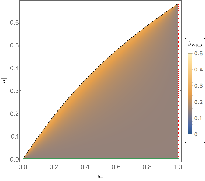
In Fig. 3 we plot $\beta_{\mathrm{WKB}}\equiv-{\rm Im}(\omega^{+}_{\mathrm{WKB}})/\kappa_{-}$ for $n=0$. For all the range of $(y_{+},|\alpha|)$ we find that $\beta_{\mathrm{WKB}}\leq 1/2$, with $\beta_{\mathrm{WKB}}=1/2$ saturated only at extremality (represented by the dashed ‘diagonal’ black line in Fig. 3). This shows that scalar field perturbations of any non-extremal Kerr-de Sitter black hole respect the strong cosmic censorship conjecture.

Of course this calculation was based on approximate (geometric optics/WKB) methods and so one could ask whether corrections to these results might push the true value of $\beta$ above $1/2$, especially near extremality. However, the corrections to ${\rm Im}(\omega)$ are of order $1/|m|$ so, for any fixed background, the corrections can be made arbitrarily small by taking $|m|$ large enough.⁵⁵ 5 In fact for vanishing $\Lambda$ the corrections to ${\rm Im}(\omega)$ are ${\cal O}(1/m^{2})$ [32] and we expect that the same is true with $\Lambda>0$. So the WKB results should be reliable for sufficiently large $|m|$. In the next section we will determine the quasinormal frequencies numerically and find that, for large enough $|m|$, the WKB result is always in excellent agreement with the exact result.

In this section we will compute numerically the quasinormal modes of a Kerr-de Sitter black hole and make a matching with the analytic results of section IV.2. We first note that the massless scalar wave equation admits separable solutions of the form (4.17), with $S_{\omega\ell m}(\chi)$ and $R_{\omega\ell m}(r)$ obeying the following two-parameter coupled eigenvalue problem

		$\displaystyle\partial_{\chi}\left[\Delta_{\chi}(\chi)\partial_{\chi}S_{\omega\ell m}(\chi)\right]-\left[\frac{\Xi^{2}}{\Delta_{\chi}(\chi)}\left(a\,m-\sigma_{\chi}\omega\right)^{2}-K\right]S_{\omega\ell m}(\chi)=0\,,$		(4.42a)
		$\displaystyle\partial_{r}\left[\Delta_{r}(r)\partial_{r}R_{\omega\ell m}(r)\right]+\left[\frac{\Xi^{2}}{\Delta_{r}(r)}\left(a\,m-\sigma_{r}\omega\right)^{2}-K\right]R_{\omega\ell m}(r)=0\,.$		(4.42b)

The symmetry exhibited by the above two equations is only achieved for the particular coordinates used in the line element (3.4). The eigenvalues to be determined are $(\omega,K)$ where $K$ arises as a separation constant. Before describing the numerical method we used, we first comment on the thorny issue of boundary conditions. Both equations have regular singular points when $\Delta_{r}$ and $\Delta_{\chi}$ vanish, so we can use Frobenius method to determine their behaviour there.

For the angular equation, we find

$$S_{\omega\ell m}(\chi)=(|a|-\chi)^{\pm\frac{|m|}{2}}\sum_{n=0}^{+\infty}(|a|-\chi)^{n}\,S_{\omega\ell m}^{(n,+)}$$

(4.43)

at $\chi=|a|$. Regularity then demands choosing the $+$ sign. A similar behaviour is found at $\chi=-|a|$:

$$S_{\omega\ell m}(\chi)=(|a|+\chi)^{\pm\frac{|m|}{2}}\sum_{n=0}^{+\infty}(|a|+\chi)^{n}\,S_{\omega\ell m}^{(n,-)}\,.$$

(4.44)

Again the upper sign leads to the physically meaningful solution. We thus conclude that we can factor out all non-analytic behaviour of $S_{\omega\ell m}$ by setting

$$S_{\omega\ell m}(\chi)=(a^{2}-\chi^{2})^{\frac{|m|}{2}}\tilde{S}_{\omega\ell m}(\chi)\,,$$

(4.45)

and solving for the smooth eigenfunction $\tilde{S}_{\omega\ell m}(\chi)$.

For the radial coordinate, we have to distinguish the cosmological horizon from the black hole horizon. At the black hole horizon a Frobenius expansion yields

$$R_{\omega\ell m}(r)=(r-r_{+})^{\pm\,\frac{i}{2\,\kappa_{+}}\left(\omega-m\,\Omega_{+}\right)}\sum_{n=0}^{+\infty}(r-r_{+})^{n}\,R_{\omega\ell m}^{(n,+)}$$

(4.46)

and regularity at the black hole event horizon, which stems from demanding a smooth expansion around $r=r_{+}$ in ingoing coordinates $(v,r,\chi,\phi^{\prime})$ at the black hole horizon, demands choosing the lower sign. For the cosmological horizon we find

$$R_{\omega\ell m}(r)=(r_{c}-r)^{\pm\,\frac{i}{2\,\kappa_{c}}\left(\omega-m\,\Omega_{c}\right)}\sum_{n=0}^{+\infty}(r_{c}-r)^{n}\,R_{\omega\ell m}^{(n,c)}\,,$$

(4.47)

and again imposing outgoing boundary conditions at the cosmological horizon demands selecting the minus sign in the expression above. We thus consider the following field redefinition:

$$R_{\omega\ell m}(r)=(r_{c}-r)^{-\,\frac{i}{2\,\kappa_{c}}\left(\omega-m\,\Omega_{c}\right)}(r-r_{+})^{-\,\frac{i}{2\,\kappa_{+}}\left(\omega-m\,\Omega_{+}\right)}\tilde{R}_{\omega\ell m}(r)$$

(4.48)

where $\tilde{R}_{\omega\ell m}(r)$ should now be a smooth function with a regular Taylor series at each of the horizons.

The procedure is now clear, we take the field redefinitions (4.45) and (4.48) and input them into Eqs. (4.42). The resulting equations are still quadratic in $\omega$ and $K$, and form a coupled eigenvalue problem with eigenfunctions $\big(\tilde{S}_{\omega\ell m}(\chi),\tilde{R}_{\omega\ell m}(r)\big)$ and eigenvalues $(\omega,K)$. The boundary conditions for $\tilde{S}_{\omega\ell m}(\chi)$ and $\tilde{R}_{\omega\ell m}(r)$ are then found by Taylor expanding the equations of motion close to either boundary, and turn out to be of the Robin type, i.e.

$$\mathcal{F}^{1,\pm}(\omega,K)\tilde{S}_{\omega\ell m}^{\prime}(\pm|a|)=\mathcal{F}^{0,\pm}(\omega,K)\tilde{S}_{\omega\ell m}(\pm|a|)$$

(4.49)

and

$$\mathcal{Q}^{1,+}(\omega,K)\tilde{R}_{\omega\ell m}^{\prime}(r_{+})=\mathcal{Q}^{+,0}(\omega,K)\tilde{R}_{\omega\ell m}(r_{+})\,,\quad\mathcal{Q}^{c,1}(\omega,K)\tilde{R}_{\omega\ell m}^{\prime}(r_{c})=\mathcal{Q}^{c,0}(\omega,K)\tilde{R}_{\omega\ell m}(r_{c})\,.$$

(4.50)

with $\mathcal{F}^{1,\pm}(\omega,K)$, $\mathcal{F}^{0,\pm}(\omega,K)$, $\mathcal{Q}^{1,+}(\omega,K)$, $\mathcal{Q}^{0,+}(\omega,K)$ $\mathcal{Q}^{1,-}(\omega,K)$ and $\mathcal{Q}^{-,+}(\omega,K)$ being known functions which are at most second order polynomials in $\omega$ and $K$. For the numerical procedure, it is also useful to consider coordinates whose range do not depend on the parameters of the solution. To achieve this, we make the following simple linear coordinate transformations

$$x=\frac{|a|+\chi}{2\,|a|}\qquad\text{and}\qquad y=\frac{1-\frac{r_{+}}{r}}{1-\frac{r_{+}}{r_{c}}}\,.$$

(4.51)

The resulting equations are then solved using a Newton-Raphson algorithm, on a unit length Chebyshev grid, as first proposed in [24] and recently detailed in [35].

Our results are shown in Fig. 4 where we take $y_{+}=1/4,1/2,3/4$ (from left to right) and plot $\beta$ as a function of $a/a_{\mathrm{ext}}$. Since we are interested in tracking photon sphere modes, we will take $m=\ell=10$. For most of the moduli space of solutions $\beta\ll 1/2$, and $\beta$ only gets close to $1/2$ near extremality. This is why in Fig. 4 we restricted the range of the horizontal axis to $a/a_{\mathrm{ext}}\in[9/10,999/1000]$. Also showing in Fig. 4 are the analytic WKB photon sphere predictions of section IV.2, see (4.41), denoted by the solid black lines. For $m=\ell=50$ (not shown in Fig. 4) we see a maximum deviation between the analytic and numerical data which is not larger than $10^{-6}$ anywhere in parameter space.

To sum up, our numerical results corroborate the analytic analysis performed in section IV.2. For the specific value of $y_{+}=1/2$, we have pushed our numerical scheme to $1-a/a_{\mathrm{ext}}=10^{-5}$ and see no deviation from the WKB result.

The absolute error in $\beta$ is not terribly important: what is important is to show that corrections to the WKB result cannot push $\beta$ above $1/2$. To this end we define

$$\Delta\beta\equiv\frac{\beta-\beta_{\mathrm{WKB}}}{\frac{1}{2}-\beta}\,.$$

(4.52)

This quantity is plotted in Fig. 5 for $y_{+}=1/2$ and $\ell=m=10$. It can be seen that, for $1-a/a_{\rm ext}$ down to $10^{-5}$ we have

$$|\Delta\beta|<10^{-3}.$$

(4.53)

Thus the WKB analysis is reliable even very close to extremality. Taking $\ell=m$ to be even larger would make $\Delta\beta$ even smaller.

The Kerr-de Sitter black hole is a Petrov type D solution. Therefore, gravitational perturbations of this geometry can be studied using the Teukolsky equation, which uses the Newman-Penrose (NP) framework [36, 37, 38, 39]. We will study perturbations using the Chambers-Moss null tetrad (3.14). For quasinormal modes we assume a separable Ansatz for the (gauge invariant) perturbed Weyl scalars

		$\displaystyle\psi_{0}\equiv\bm{\ell}^{\mu}\bm{m}^{\nu}\bm{\ell}^{\rho}\bm{m}^{\alpha}\delta C_{\mu\nu\rho\alpha}=e^{-i\omega t+im\phi}\frac{R^{(+2)}_{\omega\ell m}(r)S^{(+2)}_{\omega\ell m}(\chi)}{(r-i\chi)^{2}}\,,$		(5.54a)
		$\displaystyle\psi_{4}\equiv\bm{n}^{\mu}\bar{\bm{m}}^{\nu}\bm{n}^{\rho}\bar{\bm{m}}^{\alpha}\delta C_{\mu\nu\rho\alpha}=e^{-i\omega t+im\phi}\frac{R^{(-2)}_{\omega\ell m}(r)S^{(-2)}_{\omega\ell m}(\chi)}{(r-i\chi)^{2}}\,,$		(5.54b)

where $\delta C_{\mu\nu\rho\alpha}$ are the components of the Weyl tensor perturbation. The Teukolsky equation then reduces to the following two sets of two-parameter eigenvalue problems⁶⁶ 6 The reader interested on a complete but concise overview that discusses how the solutions of (5.55)-(5.56) allow to get information about other variables can see section 2 and appendix A of [41] (with the trading $L^{2}\to-L^{2}$).

$$\left\{\begin{array}[]{ll}\displaystyle\left[\mathcal{D}_{-1}\Delta_{r}\mathcal{D}^{\dagger}_{1}-6\left(\frac{r^{2}}{L^{2}}-i\,\Xi\,\omega\,r\right)-K^{(+2)}\right]R_{\omega\ell m}^{(+2)}(r)=0\,,&\\ \\ \displaystyle\left[\mathcal{L}_{-1}\Delta_{\chi}\mathcal{L}^{\dagger}_{1}-6\left(\frac{\chi^{2}}{L^{2}}+\Xi\,\omega\,\chi\right)+K^{(+2)}\right]S_{\omega\ell m}^{(+2)}(\chi)=0\,,&\end{array}\right.$$

(5.55)

and

$$\left\{\begin{array}[]{ll}\displaystyle\left[\mathcal{D}^{\dagger}_{-1}\Delta_{r}\mathcal{D}_{1}-6\left(\frac{r^{2}}{L^{2}}+i\,\Xi\,\omega\,r\right)-K^{(-2)}\right]R_{\omega\ell m}^{(-2)}(r)=0\,,&\\ \\ \displaystyle\left[\mathcal{L}^{\dagger}_{-1}\Delta_{\chi}\mathcal{L}_{1}-6\left(\frac{\chi^{2}}{L^{2}}-\Xi\,\omega\,\chi\right)+K^{(-2)}\right]S_{\omega\ell m}^{(-2)}(\chi)=0\,,&\end{array}\right.$$

(5.56)

where $K^{(\pm 2)}$ are separation constants and we defined the operators [39, 23]:

	$\displaystyle\hskip-42.67912pt\mathcal{D}_{n}=\partial_{r}+i\,\frac{\Xi}{\Delta_{r}}\left(ma-\omega\sigma_{r}\right)+n\,\frac{\partial_{r}\Delta_{r}}{\Delta_{r}},\qquad\mathcal{D}^{\dagger}_{n}=\partial_{r}-i\,\frac{\Xi}{\Delta_{r}}\left(ma-\omega\sigma_{r}\right)+n\,\frac{\partial_{r}\Delta_{r}}{\Delta_{r}}\,,$
	$\displaystyle\hskip-42.67912pt\mathcal{L}_{n}=\partial_{\chi}+\frac{\Xi}{\Delta_{\chi}}\left(ma-\omega\sigma_{\chi}\right)+n\,\frac{\partial_{\chi}\Delta_{\chi}}{\Delta_{\chi}},\qquad\mathcal{L}^{\dagger}_{n}=\partial_{\chi}-\frac{\Xi}{\Delta_{\chi}}\left(ma-\omega\sigma_{\chi}\right)+n\,\frac{\partial_{\chi}\Delta_{\chi}}{\Delta_{\chi}}\,.$		(5.57)

Equations (5.55) and (5.56) are isospectral⁷⁷ 7 We have explicitly checked this is the case, by computing the corresponding sets of quasinormal modes associated with each of the equations., that is to say, once appropriate boundary conditions are imposed, they give the same values of $\omega$ and $K^{(+2)}=K^{(-2)}$. So in the following section, we shall focus on the pair $\{R^{(+2)}_{\omega\ell m}(r),S^{(+2)}_{\omega\ell m}(\chi)\}$ with eigenvalues $\{\omega,K^{(+2)}\}$.

References

- [1] R. Penrose, “Singularities of spacetime” in Theoretical principles in astrophysics and relativity, Eds. N.R. Liebowitz, W.H. Reid and P.O.Vandervoort, Chicago University Press, p217-243 (1978).
- [2] M. Simpson and R. Penrose, “Internal instability in a Reissner-Nordstrom black hole,” Int. J. Theor. Phys. 7, 183 (1973). doi:10.1007/BF00792069
- [3] E. Poisson and W. Israel, “Internal structure of black holes,” Phys. Rev. D 41, 1796 (1990).
- [4] M. Dafermos, “The Interior of charged black holes and the problem of uniqueness in general relativity,” Commun. Pure Appl. Math. 58, 0445 (2005) [gr-qc/0307013].
- [5] J. Luk and S. J. Oh, “Strong cosmic censorship in spherical symmetry for two-ended asymptotically flat initial data I. The interior of the black hole region,” arXiv:1702.05715 [gr-qc].
- [6] F. Mellor and I. Moss, “Stability of Black Holes in De Sitter Space,” Phys. Rev. D 41, 403 (1990).
- [7] C. M. Chambers, “The Cauchy horizon in black hole de sitter space-times,” Annals Israel Phys. Soc. 13, 33 (1997) [gr-qc/9709025].
- [8] P. R. Brady, I. G. Moss and R. C. Myers, “Cosmic censorship: As strong as ever,” Phys. Rev. Lett. 80, 3432 (1998) [gr-qc/9801032].
- [9] A. Ori, “Inner structure of a charged black hole: An exact mass-inflation solution,” Phys. Rev. Lett. 67, 789 (1991).
- [10] D. Christodoulou, “The Formation of Black Holes in General Relativity,” EMS Monographs in Mathematics, Zurich (2009) arXiv:0805.3880 [gr-qc].
- [11] M. Dafermos, “Black holes without spacelike singularities,” Commun. Math. Phys. 332, 729 (2014) [arXiv:1201.1797 [gr-qc]].
- [12] V. Cardoso, J. L. Costa, K. Destounis, P. Hintz and A. Jansen, “Quasinormal modes and Strong Cosmic Censorship,” Phys. Rev. Lett. 120, no. 3, 031103 (2018) [arXiv:1711.10502 [gr-qc]].
- [13] P. Hintz and A. Vasy, “Analysis of linear waves near the Cauchy horizon of cosmological black holes,” J. Math. Phys. 58, no. 8, 081509 (2017) [arXiv:1512.08004 [math.AP]].
- [14] A. Sá Barreto and M. Zworski, “Distribution of resonances for spherical black holes,” Math. Res. Lett. 4 (1997), 103
- [15] J.-F. Bony and D. Häfner, “Decay and non-decay of the local energy for the wave equation on the de Sitter-Schwarzschild metric,” Comm. Math. Phys. 282 (2008), 697
- [16] S. Dyatlov, “Asymptotic distribution of quasi-normal modes for Kerr-de Sitter black holes,” Annales Henri Poincare 13 (2012) 1101 [arXiv:1101.1260 [math.AP]].
- [17] S. Dyatlov, “Asymptotics of linear waves and resonances with applications to black holes,” Commun. Math. Phys. 335 (2015) no.3, 1445 [arXiv:1305.1723 [gr-qc]].
- [18] P. Hintz and A. Vasy, “The global non-linear stability of the Kerr-de Sitter family of black holes,” arXiv:1606.04014 [math.DG].
- [19] P. Hintz, “Non-linear stability of the Kerr-Newman-de Sitter family of charged black holes,” arXiv:1612.04489 [math.AP].
- [20] J. L. Costa, P. M. Giro, J. Natário and J. D. Silva, “On the occurrence of mass inflation for the Einstein-Maxwell-scalar field system with a cosmological constant and an exponential Price law,” arXiv:1707.08975 [gr-qc].
- [21] S. Hod, “Strong cosmic censorship in charged black-hole spacetimes: As strong as ever,” arXiv:1801.07261 [gr-qc].
- [22] B. Carter, “Hamilton-Jacobi and Schrödinger separable solutions of Einstein’s equations,” Commun. Math. Phys. 10 (1968) 280.
- [23] C. M. Chambers and I. G. Moss, “Stability of the Cauchy horizon in Kerr-de Sitter space-times,” Class. Quant. Grav. 11, 1035 (1994) [gr-qc/9404015].
- [24] V. Cardoso, O. J. C. Dias, G. S. Hartnett, L. Lehner and J. E. Santos, “Holographic thermalization, quasinormal modes and superradiance in Kerr-AdS,” JHEP 1404, 183 (2014) [arXiv:1312.5323 [hep-th]].
- [25] C. J. Goebel, “Comments on the ‘vibrations’ of a black hole”, Astrophys. J. 172 (1972) L95.
- [26] V. Ferrari and B. Mashhoon, “New approach to the quasinormal modes of a black hole,” Phys. Rev. D 30 (1984) 295.
- [27] V. Ferrari and B. Mashhoon, “Oscillations of a Black Hole,” Phys. Rev. Lett. 52 (1984) no.16, 1361. doi:10.1103/PhysRevLett.52.1361
- [28] B. Mashhoon, “Stability of charged rotating black holes in the eikonal approximation,” Phys. Rev. D 31 (1985) no.2, 290.
- [29] L. Bombelli and E. Calzetta, “Chaos around a black hole,” Class. Quant. Grav. 9, 2573 (1992).
- [30] N. J. Cornish and J. J. Levin, “Lyapunov timescales and black hole binaries,” Class. Quant. Grav. 20 (2003) 1649 [gr-qc/0304056].
- [31] V. Cardoso, A. S. Miranda, E. Berti, H. Witek and V. T. Zanchin, “Geodesic stability, Lyapunov exponents and quasinormal modes,” Phys. Rev. D 79 (2009) 064016 [arXiv:0812.1806 [hep-th]].
- [32] S. R. Dolan, “The Quasinormal Mode Spectrum of a Kerr Black Hole in the Eikonal Limit,” Phys. Rev. D 82 (2010) 104003 [arXiv:1007.5097 [gr-qc]].
- [33] H. Yang, D. A. Nichols, F. Zhang, A. Zimmerman, Z. Zhang and Y. Chen, “Quasinormal-mode spectrum of Kerr black holes and its geometric interpretation,” Phys. Rev. D 86 (2012) 104006 [arXiv:1207.4253 [gr-qc]].
- [34] Z. Stuchlik and M. Calvani, “Null geodesics in black hole metrics with non-zero cosmological constant”, Gen. Rel. Grav. 23, 507 (1991)
- [35] O. J. C. Dias, J. E. Santos and B. Way, “Numerical Methods for Finding Stationary Gravitational Solutions,” Class. Quant. Grav. 33, no. 13, 133001 (2016) [arXiv:1510.02804 [hep-th]].
- [36] E. Newman and R. Penrose, “An Approach to gravitational radiation by a method of spin coefficients,” J. Math. Phys. 3 (1962) 566. Errata: 4 (1963) 998.
- [37] S. A. Teukolsky, “Rotating black holes - separable wave equations for gravitational and electromagnetic perturbations,” Phys. Rev. Lett. 29 (1972) 1114.
- [38] S. A. Teukolsky, “Perturbations of a rotating black hole. 1. Fundamental equations for gravitational electromagnetic and neutrino field perturbations,” Astrophys. J. 185 (1973) 635.
- [39] S. Chandrasekhar, The mathematical theory of black holes, (Oxford University Press, New York, 1992).
- [40] G.B. Folland, ”Introduction to partial differential equations”, 2nd Ed., Princeton University Press (1995).
- [41] O. J. C. Dias and J. E. Santos, “Boundary Conditions for Kerr-AdS Perturbations,” JHEP 1310 (2013) 156 [arXiv:1302.1580 [hep-th]].