跳到论文正文
W Papers独立论文阅读器 arXiv:1801.09408 论文正文 计算阅读时间 · 0%
引用这篇论文根据当前论文元数据生成,正式投稿前建议核对。


License: arXiv.org perpetual non-exclusive license
arXiv:1801.09408v1 [math.NA] 29 Jan 2018

Convergence of a finite-volume scheme for a degenerate cross-diffusion model for ion transportThanks: The authors have been supported by the Austrian-French Program Amadée of the Austrian Exchange Service (ÖAD). The work of the first and second authors is supported by the LABEX CEMPI (ANR-11-LABX-0007-01). The third and fourth authors acknowledge partial support from the Austrian Science Fund (FWF), grants P27352, P30000, F65, and W1245

Clément Cancès Address: Inria, Univ. Lille, CNRS, UMR 8524 - Laboratoire Paul Painlevé, F-59000 Lille Email address: clement.cances@inria.fr , Claire Chainais-Hillairet Address: Univ. Lille, CNRS, UMR 8524, Inria - Laboratoire Paul Painlevé, F-59000 Lille Email address: Claire.Chainais@math.univ-lille1.fr , Anita Gerstenmayer Address: Institute for Analysis and Scientific Computing, Vienna University of Technology, Wiedner Hauptstraße 8–10, 1040 Wien, Austria Email address: anita.gerstenmayer@tuwien.ac.at and Ansgar Jüngel Address: Institute for Analysis and Scientific Computing, Vienna University of Technology, Wiedner Hauptstraße 8–10, 1040 Wien, Austria Email address: juengel@tuwien.ac.at
Date: August 24, 2026
Abstract.

An implicit Euler finite-volume scheme for a degenerate cross-diffusion system describing the ion transport through biological membranes is analyzed. The strongly coupled equations for the ion concentrations include drift terms involving the electric potential, which is coupled to the concentrations through the Poisson equation. The cross-diffusion system possesses a formal gradient-flow structure revealing nonstandard degeneracies, which lead to considerable mathematical difficulties. The finite-volume scheme is based on two-point flux approximations with “double” upwind mobilities. It preserves the structure of the continuous model like nonnegativity, upper bounds, and entropy dissipation. The degeneracy is overcome by proving a new discrete Aubin-Lions lemma of “degenerate” type. Under suitable assumptions, the existence and uniqueness of bounded discrete solutions, a discrete entropy inequality, and the convergence of the scheme is proved. Numerical simulations of a calcium-selective ion channel in two space dimensions indicate that the numerical scheme is of first order.

Key words and phrases: 
Ion transport, finite-volume method, gradient flow, entropy method, existence of discrete solutions, convergence of the scheme, calcium-selective ion channel.
2000 Mathematics Subject Classification
65M08, 65M12, 35K51, 35K65, 35Q92.

1. Introduction

The ion transport through biological channels plays an important role in all living organisms. On a macroscopic level, the transport can be described by nonlinear partial differential equations for the ion concentrations (or, more precisely, volume fractions) and the surrounding electric potential. A classical model for ion transport are the Poisson-Nernst-Planck equations [25], which satisfy Fick’s law for the fluxes. However, this approach does not include size exclusion effects in narrow ion channels. Taking into account the finite size of the ions, one can derive from an on-lattice model in the diffusion limit another set of differential equations with fluxes depending on the gradients of all species [10, 27]. These nonlinear cross-diffusion terms are common in multicomponent systems [23, Chapter 4]. In this paper, we propose an implicit Euler finite-volume discretization of the resulting cross-diffusion system. The scheme is designed in such a way that the nonnegativity and upper bound of the concentrations as well as the entropy dissipation is preserved on the discrete level.

More specifically, the evolution of the concentrations uiu_{i} and fluxes ℱi{\mathcal{F}}_{i} of the iith ion species is governed by the equations

(1) ∂tui+divℱi=0,ℱi=−Di(u0∇ui−ui∇u0+u0uiβzi∇Φ)in Ω,t>0,\partial_{t}u_{i}+\operatorname{div}{\mathcal{F}}_{i}=0,\quad{\mathcal{F}}_{i}=-D_{i}\big(u_{0}\nabla u_{i}-u_{i}\nabla u_{0}+u_{0}u_{i}\beta z_{i}\nabla\Phi\big)\quad\mbox{in }\Omega,\ t>0,

for i=1,…,ni=1,\ldots,n, where u0=1−∑i=1nuiu_{0}=1-\sum_{i=1}^{n}u_{i} is the concentration (volume fraction) of the electro-neutral solvent, Di>0D_{i}>0 is a diffusion coefficient, β>0\beta>0 is the (scaled) inverse thermal voltage, and zi∈ℝz_{i}\in{\mathbb{R}} the charge of the iith species. Observe that we assumed Einstein’s relation which says that the quotient of the diffusion and mobility coefficients is constant, and we call this constant 1/β1/\beta. The electric potential is determined by the Poisson equation

(2) −λ2​Δ​Φ=∑i=1nzi​ui+fin ​Ω,-\lambda^{2}\Delta\Phi=\sum_{i=1}^{n}z_{i}u_{i}+f\quad\mbox{in }\Omega,

where λ2\lambda^{2} is the (scaled) permittivity constant and f=f⁡(x)f=f(x) is a permanent background charge density. Equations (1) and (2) are solved in a bounded domain Ω⊂ℝd\Omega\subset{\mathbb{R}}^{d}.

In order to match experimental conditions, the boundary ∂Ω\partial\Omega is supposed to consist of two parts, the insulating part ΓN\Gamma_{N}, on which no-flux boundary conditions are prescribed, and the union ΓD\Gamma_{D} of boundary contacts with external reservoirs, on which the concentrations are fixed. The electric potential is prescribed at the electrodes on ΓD\Gamma_{D}. This leads to the mixed Dirichlet-Neumann boundary conditions

(3) ℱi⋅ν=0on ​ΓN,\displaystyle{\mathcal{F}}_{i}\cdot\nu=0\quad\mbox{on }\Gamma_{N}, ui=u¯ion ​ΓD,i=1,…,n,\displaystyle\quad u_{i}=\overline{u}_{i}\quad\mbox{on }\Gamma_{D},\quad i=1,\ldots,n,
(4) ∇Φ⋅ν=0on ΓN,\displaystyle\nabla\Phi\cdot\nu=0\quad\mbox{on }\Gamma_{N}, Φ=Φ¯on ​ΓD,\displaystyle\quad\Phi=\overline{\Phi}\quad\mbox{on }\Gamma_{D},

where the boundary data (u¯i)1≤i≤n(\overline{u}_{i})_{1\leq i\leq n} and Φ¯{\overline{\Phi}} can be defined on the whole domain Ω\Omega. Finally, we prescribe the initial conditions

(5) ui​(⋅,0)=uiIin ​Ω,i=1,…,n.u_{i}(\cdot,0)=u_{i}^{I}\quad\mbox{in }\Omega,\ i=1,\ldots,n.

The main mathematical difficulties of equations (1) are the strong coupling and the fact that the diffusion matrix (Ai​j​(u))(A_{ij}(u)), defined by Ai​j​(u)=Di​uiA_{ij}(u)=D_{i}u_{i} for i≠ji\neq j and Ai​i​(u)=Di​(u0+ui)A_{ii}(u)=D_{i}(u_{0}+u_{i}) is not symmetric and not positive definite. It was shown in [10, 22] that system (1) possesses a formal gradient-flow structure. This means that there exists a (relative) entropy functional H⁡[u]=∫Ωh⁡(u)​𝑑xH[u]=\int_{\Omega}h(u)dx with the entropy density

h⁡(u)=∑i=0n∫u¯iuilog⁡su¯i​𝑑s+β​λ22​|∇(Φ−Φ¯)|2,h(u)=\sum_{i=0}^{n}\int_{\overline{u}_{i}}^{u_{i}}\log\frac{s}{\overline{u}_{i}}ds+\frac{\beta\lambda^{2}}{2}|\nabla(\Phi-\overline{\Phi})|^{2},

where u=(u1,…,un)u=(u_{1},\ldots,u_{n}) and u0=1−∑i=1nuiu_{0}=1-\sum_{i=1}^{n}u_{i}, such that (1) can be formally written as

∂tui=div(∑j=1nBi​j∇wj),\partial_{t}u_{i}=\operatorname{div}\bigg(\sum_{j=1}^{n}B_{ij}\nabla w_{j}\bigg),

where Bi​i=Di​u0​uiB_{ii}=D_{i}u_{0}u_{i}, Bi​j=0B_{ij}=0 for i≠ji\neq j provide a diagonal positive definite matrix, and wjw_{j} are the entropy variables, defined by

∂h∂ui=wi−w¯i,where\displaystyle\frac{\partial h}{\partial u_{i}}=w_{i}-\overline{w}_{i},\quad\mbox{where}
wi=loguiu0+βziΦ,w¯i=logu¯iu¯0+βziΦ¯,i=1,…,n.\displaystyle w_{i}=\log\frac{u_{i}}{u_{0}}+\beta z_{i}\Phi,\quad\overline{w}_{i}=\log\frac{\overline{u}_{i}}{\overline{u}_{0}}+\beta z_{i}\overline{\Phi},\quad i=1,\ldots,n.

We refer to [20, Lemma 7] for the computation of ∂h/∂ui\partial h/\partial u_{i}.

The entropy structure of (1) is useful for two reasons. First, it leads to L∞L^{\infty} bounds for the concentrations. Indeed, the transformation (u,Φ)↦w(u,\Phi)\mapsto w to entropy variables can be inverted, giving u=u⁡(w,Φ)u=u(w,\Phi) with

ui(w,Φ)=exp⁡(wi−β​zi​Φ)1+∑j=1nexp⁡(wj−β​zj​Φ),i=1,…,n.u_{i}(w,\Phi)=\frac{\exp(w_{i}-\beta z_{i}\Phi)}{1+\sum_{j=1}^{n}\exp(w_{j}-\beta z_{j}\Phi)},\quad i=1,\ldots,n.

Then uiu_{i} is positive and bounded from above, i.e.

(6) u∈𝒟={u∈(0,1)n:∑i=1nui<1}.u\in{\mathcal{D}}=\bigg\{u\in(0,1)^{n}:\sum_{i=1}^{n}u_{i}<1\bigg\}.

This yields L∞L^{\infty} bounds without the use of a maximum principle. Second, the entropy structure leads to gradient estimates via the entropy inequality

d​Hd​t+12​∫Ω∑i=1nDi​u0​ui​|∇wi|2​𝑑x≤C,\frac{dH}{dt}+\frac{1}{2}\int_{\Omega}\sum_{i=1}^{n}D_{i}u_{0}u_{i}|\nabla w_{i}|^{2}dx\leq C,

where the constant C>0C>0 depends on the Dirichlet boundary data. Because of

(7) ∑i=1nu0​ui​|∇log⁡uiu0|2=4​∑i=1nu0​|∇ui1/2|2+4​|∇u01/2|2+|∇u0|2,\sum_{i=1}^{n}u_{0}u_{i}\bigg|\nabla\log\frac{u_{i}}{u_{0}}\bigg|^{2}=4\sum_{i=1}^{n}u_{0}|\nabla u_{i}^{1/2}|^{2}+4|\nabla u_{0}^{1/2}|^{2}+|\nabla u_{0}|^{2},

we achieve gradient estimates for u01/2​uiu_{0}^{1/2}u_{i} and u01/2u_{0}^{1/2}. Since u0u_{0} may vanish locally, this does not give gradient bounds for uiu_{i}, which expresses the degenerate nature of the cross-diffusion system. As a consequence, the flux has to be formulated in the terms of gradients of u01/2​uiu_{0}^{1/2}u_{i} and u01/2u_{0}^{1/2} only, namely

(8) ℱi=−Di(u01/2∇(u01/2ui)−3u01/2ui∇u01/2+u0uiβzi∇Φ).{\mathcal{F}}_{i}=-D_{i}\big(u_{0}^{1/2}\nabla(u_{0}^{1/2}u_{i})-3u_{0}^{1/2}u_{i}\nabla u_{0}^{1/2}+u_{0}u_{i}\beta z_{i}\nabla\Phi\big).

The challenge is to derive a discrete version of this formulation. It turns out that (24) below is the right formulation in our context (assuming vanishing drift parts).

Our aim is to design a numerical approximation of (1) which preserves the structural properties of the continuous equations. This suggests to use the entropy variables as the unknowns, as it was done in our previous work [20] with simulations in one space dimension. Unfortunately, we have not been able to perform a numerical convergence analysis with these variables. The reason is that we need discrete chain rules in order to formulate (7) on the discrete level and these discrete chain rules seem to be not easily available. Therefore, we use the original variables uiu_{i} for the numerical discretization. Interestingly, we are still able to prove that the scheme preserves the nonnegativity, upper bound, and entropy inequality. However, the upper bound comes at a price: We need to assume that all diffusion coefficients DiD_{i} are the same. Under this assumption, u0=1−∑i=1nuiu_{0}=1-\sum_{i=1}^{n}u_{i} solves a drift-diffusion equation for which the (discrete) maximum principle can be applied. It is not surprising that the L∞L^{\infty} bound can be shown only under an additional condition, since cross-diffusion systems usually do not allow for a maximum principle.

The key observation for the numerical discretization is that the fluxes can be written on each cell in a “double” drift-diffusion form, i.e., both ℱi=−Di(u0∇ui−uiVi){\mathcal{F}}_{i}=-D_{i}(u_{0}\nabla u_{i}-u_{i}V_{i}) and Vi=∇u0−βziu0∇ΦV_{i}=\nabla u_{0}-\beta z_{i}u_{0}\nabla\Phi have the structure ∇v+v​F\nabla v+vF, where ∇v\nabla v is the diffusion term and v​FvF is the drift term. We discretize ℱ{\mathcal{F}} and VV by using a two-point flux aproximation with “double” upwind mobilities.

Our analytical results are stated and proved for no-flux boundary conditions on ∂Ω\partial\Omega. Mixed Dirichlet-Neumann boundary conditions could be prescribed as well, but the proofs would become even more technical. The main results are as follows.

  • •

    We prove the existence of solutions to the fully discrete numerical scheme (Theorem 1). If the drift part vanishes, the solution is unique. The existence proof uses a topological degree argument in finite space dimensions, while the uniqueness proof is based on the entropy method of Gajewski [18], recently extended to cross-diffusion systems [20, 28].

  • •

    Thanks to the “double” upwind structure, the scheme preserves the nonnegativity and upper bound for the concentrations (at least if Di=DD_{i}=D for all ii). Moreover, convexity arguments show that the discrete entropy is dissipated with a discrete entropy production analogous to (7) (Theorem 2). The proof of the discrete entropy inequality only works if the drift term vanishes, since we need to control a discrete version of the sum ∑i=1nui\sum_{i=1}^{n}u_{i} from below; see the discussion after Theorem 2.

  • •

    The discrete solutions converge to the continuous solutions to (1) as the mesh size tends to zero (Theorem 3). The proof is based on a priori estimates obtained from the discrete entropy inequality. The compactness is derived from a new discrete Aubin-Lions lemma, which takes into account the nonstandard degeneracy of the equations; see Lemma 10 in the appendix.

  • •

    Numerical experiments for a calcium-selective ion channel in two space dimensions show the dynamical behavior of the solutions and their large-time asymptotics to the equilibrium. The tests indicate that the order of convergence in the L1L^{1} norm is one.

In the literature, there exist some results on finite-volume schemes for cross-diffusion systems. An upwind two-point flux approximation similar to our discretization was recently used in [1] for a seawater intrusion cross-diffusion model. A two-point flux approximation with a nonlinear positivity-preserving approximation of the cross-diffusion coefficients, modeling the segregation of a two-species population, was suggested in [4], assuming positive definiteness of the diffusion matrix. The Laplacian structure of the population model (still for positive definite matrices) was exploited in [24] to design a convergent linear finite-volume scheme, which avoids fully implicit approximations. A semi-implicit finite-volume discretization for a biofilm model with a nonlocal time integrator was proposed in [26]. Finite-volume schemes for cross-diffusion systems with nonlocal (in space) terms were also analyzed; see, for instance, [3] for a food chain model and [2] for an epidemic model. Moreover, a finite-volume scheme for a Keller-Segel system with additional cross diffusion and discrete entropy dissipation property was investigated in [7]. All these models, however, do not include volume filling and do not possess the degenerate structure explained before.

The paper is organized as follows. The numerical scheme and the main results are presented in Section 2. In Section 3, the existence and uniqueness of bounded discrete solutions are shown. We prove the discrete entropy inequality and further a priori estimates in Section 4, while Section 5 is concerned with the convergence of the numerical scheme. Numerical experiments are given in Section 6 in order to illustrate the order of convergence and the long time behavior of the scheme. For the compactness arguments, we need two discrete Aubin-Lions lemmas which are proved in the appendix.

2. Numerical scheme and main results

2.1. Notations and definitions

We summarize our general hypotheses on the data:

  • (H1)

    Domain: Ω⊂ℝd\Omega\subset{\mathbb{R}}^{d} (d=2d=2 or d=3d=3) is an open, bounded, polygonal domain with ∂Ω=ΓD∪ΓN∈C0,1\partial\Omega=\Gamma_{D}\cup\Gamma_{N}\in C^{0,1}, ΓD∩ΓN=∅\Gamma_{D}\cap\Gamma_{N}=\emptyset.

  • (H2)

    Parameters: T>0T>0, Di>0D_{i}>0, β>0\beta>0, and zi∈ℝz_{i}\in{\mathbb{R}}, i=1,…,ni=1,\ldots,n.

  • (H3)

    Background charge: f∈L∞​(Ω)f\in L^{\infty}(\Omega).

  • (H4)

    Initial and boundary data: uiI∈L∞​(Ω)u_{i}^{I}\in L^{\infty}(\Omega), u¯i∈H1​(Ω)\overline{u}_{i}\in H^{1}(\Omega) satisfy uiI≥0u_{i}^{I}\geq 0, u¯i≥0\overline{u}_{i}\geq 0 and 1−∑i=1nuiI≥01-\sum_{i=1}^{n}u_{i}^{I}\geq 0, 1−∑i=1nu¯i≥01-\sum_{i=1}^{n}\overline{u}_{i}\geq 0 in Ω\Omega for i=1,…,ni=1,\ldots,n, and Φ¯∈H1​(Ω)∩L∞​(Ω)\overline{\Phi}\in H^{1}(\Omega)\cap L^{\infty}(\Omega).

For our main results, we need additional technical assumptions:

  • (A1)

    ∂Ω=ΓN\partial\Omega=\Gamma_{N}, i.e., we impose no-flux boundary conditions on the whole boundary.

  • (A2)

    The diffusion constants are equal, Di=D>0D_{i}=D>0 for i=1,…,ni=1,\ldots,n.

  • (A3)

    The drift terms are set to zero, Φ≡0\Phi\equiv 0.

Remark 1 (Discussion of the assumptions).

Assumption (A1) is supposed for simplicity only. Mixed Dirichlet-Neumann boundary conditions can be included in the analysis (see, e.g., [20]), but the proofs become even more technical. Mixed boundary conditions are chosen in the numerical experiments; therefore, the numerical scheme is defined for that case. Assumption (A2) is needed for the derivation of an upper bound for the solvent concentration. Indeed, when Di=DD_{i}=D for all ii, summing (1) over i=1,…,ni=1,\ldots,n gives

∂tu0=Ddiv(∇u0−u0w∇Φ),where w=β∑i=1nziui.\partial_{t}u_{0}=D\operatorname{div}(\nabla u_{0}-u_{0}w\nabla\Phi),\quad\mbox{where }w=\beta\sum_{i=1}^{n}z_{i}u_{i}.

On the discrete level, we replace u0w∇Φu_{0}w\nabla\Phi by an upwind approximation. This allows us to apply the discrete maximum principle showing that u0≥0u_{0}\geq 0 and hence u=(u1,…,un)∈𝒟¯u=(u_{1},\ldots,u_{n})\in\overline{{\mathcal{D}}} with 𝒟{\mathcal{D}} defined in (6). Finally, Assumption (A3) is needed to derive a discrete version of the entropy inequality. Without the drift terms, the upwinding value does not depend on the index of the species, which simplifies some expressions; see Remark 2. ∎

For the definition of the numerical scheme for (1)-(2), we need to introduce a suitable discretization of the domain Ω\Omega and the interval (0,T)(0,T). For simplicity, we consider a uniform time discretization with time step △​t>0{\triangle t}>0, and we set tk=k​△​tt^{k}=k{\triangle t} for k=1,…,Nk=1,\ldots,N, where T>0T>0, N∈ℕN\in{\mathbb{N}} are given and △​t=T/N{\triangle t}=T/N. The domain Ω\Omega is discretized by a regular and admissible triangulation in the sense of [16, Definition 9.1]. The triangulation consists of a family 𝒯{\mathcal{T}} of open polygonal convex subsets of Ω\Omega (so-called cells), a family ℰ{\mathcal{E}} of edges (or faces in three dimensions), and a family of points (xK)K∈𝒯(x_{K})_{K\in{\mathcal{T}}} associated to the cells. The admissibility assumption implies that the straight line between two centers of neighboring cells xK​xL¯\overline{x_{K}x_{L}} is orthogonal to the edge σ=K|L\sigma=K|L between two cells KK and LL. The condition is satisfied by, for instance, triangular meshes whose triangles have angles smaller than π/2\pi/2 [16, Examples 9.1] or Voronoi meshes [16, Example 9.2].

We assume that the family of edges ℰ{\mathcal{E}} can be split into internal and external edges ℰ=ℰint∪ℰext{\mathcal{E}}={\mathcal{E}}_{\rm int}\cup{\mathcal{E}}_{\rm ext} with ℰint={σ∈ℰ:σ⊂Ω}{\mathcal{E}}_{\rm int}=\{\sigma\in{\mathcal{E}}:\sigma\subset\Omega\} and ℰext={σ∈ℰ:σ⊂∂Ω}{\mathcal{E}}_{\rm ext}=\{\sigma\in{\mathcal{E}}:\sigma\subset\partial\Omega\}. Each exterior edge is assumed to be an element of either the Dirichlet or Neumann boundary, i.e. ℰext=ℰextD∪ℰextN{\mathcal{E}}_{\rm ext}={\mathcal{E}}_{\rm ext}^{D}\cup{\mathcal{E}}_{\rm ext}^{N}. For given K∈𝒯K\in{\mathcal{T}}, we define the set ℰK{\mathcal{E}}_{K} of the edges of KK, which is the union of internal edges and edges on the Dirichlet or Neumann boundary, and we set ℰK,int=ℰK∩ℰint{\mathcal{E}}_{K,\rm int}={\mathcal{E}}_{K}\cap{\mathcal{E}}_{\rm int}.

The size of the mesh is defined by h⁡(𝒯)=sup{diam⁡(K):K∈𝒯}h({\mathcal{T}})=\sup\{\operatorname{diam}(K):K\in{\mathcal{T}}\}. For σ∈ℰint\sigma\in{\mathcal{E}}_{\rm int} with σ=K|L\sigma=K|L, we denote by dσ=d⁡(xK,xL){\mathrm{d}}_{\sigma}={\mathrm{d}}(x_{K},x_{L}) the Euclidean distance between xKx_{K} and xLx_{L}, while for σ∈ℰext\sigma\in{\mathcal{E}}_{\rm ext}, we set dσ=d⁡(xK,σ){\mathrm{d}}_{\sigma}=d(x_{K},\sigma). For a given edge σ∈ℰ\sigma\in{\mathcal{E}}, the transmissibility coefficient is defined by

(9) τσ=m⁡(σ)dσ,\tau_{\sigma}=\frac{\mathrm{m}(\sigma)}{{\mathrm{d}}_{\sigma}},

where m⁡(σ)\mathrm{m}(\sigma) denotes the Lebesgue measure of σ\sigma.

We impose a regularity assumption on the mesh: There exists ζ>0\zeta>0 such that for all K∈𝒯K\in{\mathcal{T}} and σ∈ℰK\sigma\in{\mathcal{E}}_{K}, it holds that

(10) d⁡(xK,σ)≥ζ​dσ.{\mathrm{d}}(x_{K},\sigma)\geq\zeta{\mathrm{d}}_{\sigma}.

This hypothesis is needed to apply discrete functional inequalities (see [6, 16]) and a discrete compactness theorem (see [19]).

It remains to introduce suitable function spaces for the numerical discretization. The space ℋ𝒯\mathcal{H}_{\mathcal{T}} of piecewise constant functions is defined by

ℋ𝒯={v:Ω¯→ℝ:∃(vK)K∈𝒯⊂ℝ,v(x)=∑K∈𝒯vK𝟏K(x)}.\mathcal{H}_{\mathcal{T}}=\bigg\{v:\overline{\Omega}\to{\mathbb{R}}:\exists(v_{K})_{K\in{\mathcal{T}}}\subset{\mathbb{R}},\ v(x)=\sum_{K\in{\mathcal{T}}}v_{K}\mathbf{1}_{K}(x)\bigg\}.

The (squared) discrete H1H^{1} norm on this space is given by

(11) ‖v‖1,𝒯2=∑σ=K|L∈ℰintτσ​(vK−vL)2+∑K∈𝒯m⁡(K)​vK2.\|v\|_{1,{\mathcal{T}}}^{2}=\sum_{\sigma=K|L\in{\mathcal{E}}_{\rm int}}\tau_{\sigma}(v_{K}-v_{L})^{2}+\sum_{K\in{\mathcal{T}}}\mathrm{m}(K)v_{K}^{2}.

The discrete H−1H^{-1} norm is the dual norm with respect to the L2L^{2} scalar product,

(12) ∥v∥−1,𝒯=sup{∫Ωvwdx:w∈ℋ𝒯,∥w∥1,𝒯=1}.\|v\|_{-1,{\mathcal{T}}}=\sup\bigg\{\int_{\Omega}vwdx:w\in\mathcal{H}_{\mathcal{T}},\ \|w\|_{1,{\mathcal{T}}}=1\bigg\}.

Then

|∫Ωv​w​𝑑x|≤‖v‖−1,𝒯​‖w‖1,𝒯for ​v,w∈ℋ𝒯.\bigg|\int_{\Omega}vwdx\bigg|\leq\|v\|_{-1,{\mathcal{T}}}\|w\|_{1,{\mathcal{T}}}\quad\mbox{for }v,w\in\mathcal{H}_{\mathcal{T}}.

Finally, we introduce the space ℋ𝒯,△​t\mathcal{H}_{{\mathcal{T}},{\triangle t}} of piecewise constant in time functions with values in ℋ𝒯\mathcal{H}_{\mathcal{T}},

ℋ𝒯,△​t={v:Ω¯×[0,T]→ℝ:∃(vk)k=1,…,N⊂ℋ𝒯,v(x,t)=∑k=1Nvk(x)𝟏(tk−1,tk)(t)},\mathcal{H}_{{\mathcal{T}},{\triangle t}}=\bigg\{v:\overline{\Omega}\times[0,T]\to{\mathbb{R}}:\exists(v^{k})_{k=1,\ldots,N}\subset\mathcal{H}_{\mathcal{T}},\ v(x,t)=\sum_{k=1}^{N}v^{k}(x)\mathbf{1}_{(t^{k-1},t^{k})}(t)\bigg\},

equipped with the discrete L2​(0,T,H1​(Ω))L^{2}(0,T;H^{1}(\Omega)) norm

‖v‖1,𝒯,△​t=(∑k=1N△​t​‖vk‖1,𝒯2)1/2.\|v\|_{1,{\mathcal{T}},{\triangle t}}=\bigg(\sum_{k=1}^{N}{\triangle t}\|v^{k}\|_{1,{\mathcal{T}}}^{2}\bigg)^{1/2}.

For the numerical scheme, we introduce some further definitions. Let ui∈ℋ𝒯u_{i}\in\mathcal{H}_{\mathcal{T}} with values u¯i,σ\overline{u}_{i,\sigma} on the Dirichlet boundary (i=1,…,ni=1,\ldots,n). Then we introduce

(13) DK,σ​(ui)=ui,K,σ−ui,K,\displaystyle\text{D}_{K,\sigma}(u_{i})=u_{i,K,\sigma}-u_{i,K},
whereui,K,σ={ui,L for ​σ∈ℰint,σ=K|L,u¯i,σ for ​σ∈ℰext,KD,ui,K for ​σ∈ℰext,KN,u¯i,σ=1m⁡(σ)​∫σu¯i​𝑑s.\displaystyle\mbox{where}\quad u_{i,K,\sigma}=\begin{cases}u_{i,L}\quad&\text{ for }\sigma\in{\mathcal{E}}_{\rm int},\ \sigma=K|L,\\ \overline{u}_{i,\sigma}\quad&\text{ for }\sigma\in{\mathcal{E}}^{D}_{{\rm ext},K},\\ u_{i,K}&\text{ for }\sigma\in{\mathcal{E}}^{N}_{{\rm ext},K},\end{cases}\quad\overline{u}_{i,\sigma}=\frac{1}{\mathrm{m}(\sigma)}\int_{\sigma}\overline{u}_{i}ds.

The numerical fluxes ℱK,σ{\mathcal{F}}_{K,\sigma} should be consistent approximations to the exact fluxes through the edges ∫σℱ⋅ν​𝑑s\int_{\sigma}{\mathcal{F}}\cdot\nu ds. We impose the conservation of the numerical fluxes ℱK,σ+ℱL,σ=0{\mathcal{F}}_{K,\sigma}+{\mathcal{F}}_{L,\sigma}=0 for edges σ=K|L\sigma=K|L, requiring that they vanish on the Neumann boundary edges, ℱK,σ=0{\mathcal{F}}_{K,\sigma}=0 for σ∈ℰext,KN\sigma\in{\mathcal{E}}_{{\rm ext},K}^{N}. Then the discrete integration-by-parts formula becomes for u∈ℋ𝒯u\in\mathcal{H}_{\mathcal{T}}

∑K∈𝒯∑σ∈ℰKℱK,σuK=−∑σ∈ℰℱK,σDK,σ(u)+∑σ∈ℰextDℱK,σuK,σ.\sum_{K\in{\mathcal{T}}}\sum_{\sigma\in{\mathcal{E}}_{K}}{\mathcal{F}}_{K,\sigma}u_{K}=-\sum_{\sigma\in{\mathcal{E}}}{\mathcal{F}}_{K,\sigma}\textrm{D}_{K,\sigma}(u)+\sum_{\sigma\in{\mathcal{E}}_{\rm ext}^{D}}{\mathcal{F}}_{K,\sigma}u_{K,\sigma}.

When ∂Ω=ΓN\partial\Omega=\Gamma_{N}, this formula simplifies to

(14) ∑K∈𝒯∑σ∈ℰKℱK,σ​uK=∑σ=K|L∈ℰintℱK,σ​(uK−uL).\sum_{K\in{\mathcal{T}}}\sum_{\sigma\in{\mathcal{E}}_{K}}{\mathcal{F}}_{K,\sigma}u_{K}=\sum_{\sigma=K|L\in{\mathcal{E}}_{\rm int}}{\mathcal{F}}_{K,\sigma}(u_{K}-u_{L}).

2.2. Numerical scheme

We need to approximate the initial, boundary, and given functions on the elements K∈𝒯K\in{\mathcal{T}} and edges σ∈ℰ\sigma\in{\mathcal{E}}:

ui,KI\displaystyle u^{I}_{i,K} =1m⁡(K)​∫KuiI​(x)​𝑑x,\displaystyle=\frac{1}{\mathrm{m}(K)}\int_{K}u^{I}_{i}(x)dx, fK\displaystyle f_{K} =1m⁡(K)​∫Kf⁡(x)​𝑑x,\displaystyle=\frac{1}{\mathrm{m}(K)}\int_{K}f(x)dx,
u¯i,σ\displaystyle\overline{u}_{i,\sigma} =1m⁡(σ)​∫σu¯i​𝑑s,\displaystyle=\frac{1}{\mathrm{m}(\sigma)}\int_{\sigma}\overline{u}_{i}ds, Φ¯σ\displaystyle\overline{\Phi}_{\sigma} =1m⁡(σ)​∫σΦ¯​𝑑s,\displaystyle=\frac{1}{\mathrm{m}(\sigma)}\int_{\sigma}\overline{\Phi}ds,

and we set u0,KI=1−∑i=1nui,KIu_{0,K}^{I}=1-\sum_{i=1}^{n}u_{i,K}^{I} and u¯0,σ=1−∑i=1nu¯i,σ\overline{u}_{0,\sigma}=1-\sum_{i=1}^{n}\overline{u}_{i,\sigma}.

The numerical scheme is as follows. Let K∈𝒯K\in{\mathcal{T}}, k∈{1,…,N}k\in\{1,\ldots,N\}, i=1,…,ni=1,\ldots,n, and ui,Kk−1≥0u_{i,K}^{k-1}\geq 0 be given. Then the values ui,Kku_{i,K}^{k} are determined by the implicit Euler scheme

(15) m⁡(K)​ui,Kk−ui,Kk−1△​t+∑σ∈ℰKℱi,K,σk=0,\mathrm{m}(K)\frac{u_{i,K}^{k}-u_{i,K}^{k-1}}{{\triangle t}}+\sum_{\sigma\in{\mathcal{E}}_{K}}{\mathcal{F}}_{i,K,\sigma}^{k}=0,

where the fluxes ℱi,K,σk{\mathcal{F}}_{i,K,\sigma}^{k} are given by the upwind scheme

(16) ℱi,K,σk=−τσ​Di​(u0,σk​DK,σ​(uik)−ui,σk​(DK,σ​(u0k)−u^0,σ,ik​β​zi​DK,σ​(Φk))),{\mathcal{F}}_{i,K,\sigma}^{k}=-\tau_{\sigma}D_{i}\Big(u_{0,\sigma}^{k}\text{D}_{K,\sigma}(u_{i}^{k})-u_{i,\sigma}^{k}\big(\text{D}_{K,\sigma}(u_{0}^{k})-\widehat{u}_{0,\sigma,i}^{k}\beta z_{i}\text{D}_{K,\sigma}(\Phi^{k})\big)\Big),

where τσ\tau_{\sigma} is defined in (9),

(17) u0,Kk=1−∑i=1nui,Kk,u0,σk=max⁡{u0,Kk,u0,Lk},\displaystyle u_{0,K}^{k}=1-\sum_{i=1}^{n}u_{i,K}^{k},\quad u_{0,\sigma}^{k}=\max\{u_{0,K}^{k},u_{0,L}^{k}\},
(18) ui,σk={ui,Kkif ​𝒱i,K,σk≥0,ui,K,σkif ​𝒱i,K,σk<0,,u^0,σ,ik={u0,Kkif ​zi​DK,σ​(Φk)≥0,u0,K,σkif ​zi​DK,σ​(Φk)<0,,\displaystyle u^{k}_{i,\sigma}=\begin{cases}u^{k}_{i,K}\quad&\text{if }{\mathcal{V}}^{k}_{i,K,\sigma}\geq 0,\\ u^{k}_{i,K,\sigma}&\text{if }{\mathcal{V}}^{k}_{i,K,\sigma}<0,\end{cases},\quad\widehat{u}_{0,\sigma,i}^{k}=\begin{cases}u^{k}_{0,K}\quad&\text{if }z_{i}\text{D}_{K,\sigma}(\Phi^{k})\geq 0,\\ u^{k}_{0,K,\sigma}&\text{if }z_{i}\text{D}_{K,\sigma}(\Phi^{k})<0,\end{cases},

and 𝒱i,K,σk{\mathcal{V}}_{i,K,\sigma}^{k} is the “drift part” of the flux,

(19) 𝒱i,K,σk=DK,σ​(u0k)−u^0,σ,ik​β​zi​DK,σ​(Φk){\mathcal{V}}_{i,K,\sigma}^{k}=\text{D}_{K,\sigma}(u_{0}^{k})-\widehat{u}_{0,\sigma,i}^{k}\beta z_{i}\text{D}_{K,\sigma}(\Phi^{k})

for i=1,…,ni=1,\ldots,n. Observe that we employed a double upwinding: one related to the electric potential, defining u^0,σ,ik\widehat{u}_{0,\sigma,i}^{k}, and another one related to the drift part of the flux, 𝒱i,K,σk{\mathcal{V}}_{i,K,\sigma}^{k}. The potential is computed via

(20) −λ2∑σ∈ℰKτσDK,σ(Φk)=m(K)(∑i=1nziui,Kk+fK).-\lambda^{2}\sum_{\sigma\in{\mathcal{E}}_{K}}\tau_{\sigma}\text{D}_{K,\sigma}(\Phi^{k})=\mathrm{m}(K)\bigg(\sum_{i=1}^{n}z_{i}u_{i,K}^{k}+f_{K}\bigg).

We recall that the numerical boundary conditions are given by u¯i,σ\overline{u}_{i,\sigma} and Φ¯σ\overline{\Phi}_{\sigma} for σ∈ℰextD\sigma\in{\mathcal{E}}_{\rm ext}^{D}.

We denote by ui,𝒯,△​tu_{i,{\mathcal{T}},{\triangle t}}, Φ𝒯,△​t\Phi_{{\mathcal{T}},{\triangle t}} the functions in ℋ𝒯,△​t\mathcal{H}_{{\mathcal{T}},{\triangle t}} associated to the values ui,Kku_{i,K}^{k} and ΦKk\Phi_{K}^{k}, respectively. Moreover, when dealing with a sequence of meshes (𝒯m)m({\mathcal{T}}_{m})_{m} and a sequence of time steps (△​tm)m({\triangle t}_{m})_{m}, we set ui,m=ui,𝒯m,△​tmu_{i,m}=u_{i,{\mathcal{T}}_{m},{\triangle t}_{m}}, Φm=Φ𝒯m,△​tm\Phi_{m}=\Phi_{{\mathcal{T}}_{m},{\triangle t}_{m}}.

Remark 2 (Simplified numerical scheme).

When Assumptions (A1)-(A3) hold, the numerical scheme simplifies to

(21) m⁡(K)​ui,Kk−ui,Kk−1△​t+∑σ∈ℰK,intℱi,K,σk=0,\displaystyle\mathrm{m}(K)\frac{u_{i,K}^{k}-u_{i,K}^{k-1}}{{\triangle t}}+\sum_{\sigma\in{\mathcal{E}}_{K,\rm int}}{\mathcal{F}}_{i,K,\sigma}^{k}=0,
(22) ℱi,K,σk=−τσ​D​(u0,σk​(ui,Lk−ui,Kk)−ui,σk​(u0,Lk−u0,Kk)),\displaystyle{\mathcal{F}}_{i,K,\sigma}^{k}=-\tau_{\sigma}D\Big(u_{0,\sigma}^{k}\big(u_{i,L}^{k}-u_{i,K}^{k}\big)-u_{i,\sigma}^{k}\big(u_{0,L}^{k}-u_{0,K}^{k}\big)\Big),

where u0,Kku_{0,K}^{k} and u0,σku_{0,\sigma}^{k} are defined in (17), and the definition of ui,σku_{i,\sigma}^{k} simplifies to

ui,σk={ui,Kkif ​u0,Kk−u0,Lk≤0,ui,Lkif ​u0,Kk−u0,Lk>0.u_{i,\sigma}^{k}=\begin{cases}u_{i,K}^{k}&\quad\text{if }u_{0,K}^{k}-u_{0,L}^{k}\leq 0,\\ u_{i,L}^{k}&\quad\text{if }u_{0,K}^{k}-u_{0,L}^{k}>0.\end{cases}

In the definition of ui,σku_{i,\sigma}^{k}, the upwinding value does not depend on ii anymore such that

(23) ∑i=0nui,σk=1+max⁡{u0,Kk,u0,Lk}−min⁡{u0,Kk,u0,Lk}=1+|u0,Kk−u0,Lk|.\sum_{i=0}^{n}u_{i,\sigma}^{k}=1+\max\{u_{0,K}^{k},u_{0,L}^{k}\}-\min\{u_{0,K}^{k},u_{0,L}^{k}\}=1+|u_{0,K}^{k}-u_{0,L}^{k}|.

This property is needed to control the sum ∑i=1nui,σk\sum_{i=1}^{n}u_{i,\sigma}^{k} from below in the proof of the discrete entropy inequality; see (35). Finally, we are able to reformulate the discrete fluxes such that we obtain a discrete version of (8) (without the drift part):

(24) ℱi,K,σ=τσ​D​{u0,σ1/2​(u0,K1/2​ui,K−u0,L1/2​ui,L)−ui,σ​(u0,K1/2−u0,L1/2)​(u0,σ1/2+2​u0,K1/2+u0,L1/22)}.{\mathcal{F}}_{i,K,\sigma}=\tau_{\sigma}D\bigg\{u_{0,\sigma}^{1/2}\big(u_{0,K}^{1/2}u_{i,K}-u_{0,L}^{1/2}u_{i,L}\big)-u_{i,\sigma}\big(u_{0,K}^{1/2}-u_{0,L}^{1/2}\big)\bigg(u_{0,\sigma}^{1/2}+2\frac{u_{0,K}^{1/2}+u_{0,L}^{1/2}}{2}\bigg)\bigg\}.

This formulation is needed in the convergence analysis. ∎

2.3. Main results

Since our scheme is implicit and nonlinear, the existence of an approximate solution is nontrivial. Therefore, our first result concerns the well-posedness of the numerical scheme.

Theorem 1 (Existence and uniqueness of solutions).

Let (H1)-(H4) and (A2) hold. Then there exists a solution (u,Φ)(u,\Phi) to scheme (15)-(20) satisfying uk∈𝒟¯u^{k}\in\overline{{\mathcal{D}}} and, if the initial data lie in 𝒟{\mathcal{D}}, uk∈𝒟u^{k}\in{\mathcal{D}}. If additionally Assumptions (A1) and (A3) hold, the solution is unique.

Assumption (A2) is needed to show that u0k=1−∑i=1nuiku_{0}^{k}=1-\sum_{i=1}^{n}u_{i}^{k} is nonnegative. Indeed, summing (15) and (16) over i=1,….ni=1,\ldots.n, we obtain

m(K)u0,Kk−u0,Kk−1△​t=−∑σ∈ℰKτσ(u0,σkDK,σ(∑i=1nDiuik)−∑i=1nDiui,σk𝒱i,K,σk).\mathrm{m}(K)\frac{u_{0,K}^{k}-u_{0,K}^{k-1}}{{\triangle t}}=-\sum_{\sigma\in{\mathcal{E}}_{K}}\tau_{\sigma}\bigg(u_{0,\sigma}^{k}\textrm{D}_{K,\sigma}\bigg(\sum_{i=1}^{n}D_{i}u_{i}^{k}\bigg)-\sum_{i=1}^{n}D_{i}u_{i,\sigma}^{k}\mathcal{V}_{i,K,\sigma}^{k}\bigg).

Under Assumption (A2), it follows that ∑i=1nDi​ui,Kk=D⁡(1−u0,Kk)\sum_{i=1}^{n}D_{i}u_{i,K}^{k}=D(1-u_{0,K}^{k}), and we can apply the discrete minimum principle, which then implies an L∞L^{\infty} bound for uiku_{i}^{k}. This bound allows us to apply a topological degree argument; see [13, 14]. For the uniqueness proof, we additionally need Assumption (A3), since we use the entropy method of Gajewski [18], and it seems that this method cannot be applied to cross-diffusion systems including drift terms [28]. The idea is to prove first the uniqueness of u0ku_{0}^{k}, which solves a discrete nonlinear equation, and then to show the uniqueness of uiku_{i}^{k} for i=1,…,ni=1,\ldots,n by introducing a semimetric d⁡(uk,vk)d(u^{k},v^{k}) for two solutions uk=(u1k,…,unk)u^{k}=(u_{1}^{k},\ldots,u_{n}^{k}) and vk=(v1k,…,vnk)v^{k}=(v_{1}^{k},\ldots,v_{n}^{k}) and showing that it is monotone in kk, such that a discrete Gronwall argument implies that uk=vku^{k}=v^{k}.

The second result shows that the scheme preserves a discrete version of the entropy inequality.

Theorem 2 (Discrete entropy inequality).

Let Assumptions (H1)-(H4) and (A1)-(A3) hold. Then the solution to scheme (21)-(22) constructed in Theorem 1 satisfies the discrete entropy inequality

(25) Hk−Hk−1△​t+Ik≤0,\frac{H^{k}-H^{k-1}}{{\triangle t}}+I^{k}\leq 0,

with the discrete entropy

(26) Hk=∑K∈𝒯m⁡(K)​∑i=0n(ui,Kk​(log⁡ui,Kk−1)+1)H^{k}=\sum_{K\in{\mathcal{T}}}\mathrm{m}(K)\sum_{i=0}^{n}\big(u_{i,K}^{k}(\log u_{i,K}^{k}-1)+1\big)

and the discrete entropy production

Ik\displaystyle I^{k} =D​∑σ=K|L∈ℰintτσ​(4​∑i=1nu0,σk​((ui,Kk)1/2−(ui,Lk)1/2)2CLOSE\displaystyle=D\sum_{\sigma=K|L\in{\mathcal{E}}_{\rm int}}\tau_{\sigma}\bigg(4\sum_{i=1}^{n}u_{0,\sigma}^{k}\big((u_{i,K}^{k})^{1/2}-(u_{i,L}^{k})^{1/2}\big)^{2}
OPEN+4​((u0,Kk)1/2−(u0,Lk)1/2)2+(u0,Kk−u0,Lk)2).\displaystyle\phantom{xx}{}+4\big((u_{0,K}^{k})^{1/2}-(u_{0,L}^{k})^{1/2}\big)^{2}+\big(u_{0,K}^{k}-u_{0,L}^{k}\big)^{2}\bigg).

Assumption (A3) is required to estimate the expression ∑i=1nui,σk\sum_{i=1}^{n}u_{i,\sigma}^{k}. In the continuous case, this sum equals 1−u01-u_{0}. On the discrete level, this identity cannot be expected since the value of ui,σku_{i,\sigma}^{k} depends on the upwinding value; see (18). If the drift part vanishes, the upwinding value does not depend on ii, as mentioned in Remark 2, and we can derive the estimate ∑i=1nui,σk≥1−u0,σk\sum_{i=1}^{n}u_{i,\sigma}^{k}\geq 1-u_{0,\sigma}^{k}; see Section 4.1. Note that the entropy production IkI^{k} is the discrete counterpart of (7).

The main result of this paper is the convergence of the approximate solutions to a solution to the continuous cross-diffusion system.

Theorem 3 (Convergence of the approximate solution).

Let (H1)-(H4) and (A1)-(A3) hold and let (𝒯m)({\mathcal{T}}_{m}) and (△​tm)({\triangle t}_{m}) be sequences of admissible meshes and time steps, respectively, such that h⁡(𝒯m)→0h({\mathcal{T}}_{m})\to 0 and △​tm→0{\triangle t}_{m}\to 0 as m→∞m\to\infty. Let (u0,m,…,un,m)(u_{0,m},\ldots,u_{n,m}) be the solution to (21)-(22) constructed in Theorem 1. Then there exist functions u0u_{0}, u=(u1,…,un)u=(u_{1},\ldots,u_{n}) satisfying u⁡(x,t)∈𝒟¯u(x,t)\in\overline{{\mathcal{D}}},

u01/2,u01/2​ui∈L2​(0,T,H1​(Ω)),i=1,…,n,\displaystyle u_{0}^{1/2},\ u_{0}^{1/2}u_{i}\in L^{2}(0,T;H^{1}(\Omega)),\quad i=1,\ldots,n,
u0,m1/2→u01/2,u0,m1/2ui,m→u01/2uistrongly in L2(Ω×(0,T)),\displaystyle u_{0,m}^{1/2}\to u_{0}^{1/2},\ u_{0,m}^{1/2}u_{i,m}\to u_{0}^{1/2}u_{i}\quad\mbox{strongly in }L^{2}(\Omega\times(0,T)),

where uu is a weak solution to (1), (3)-(5) (with ΓN=∂Ω\Gamma_{N}=\partial\Omega), i.e., for all ϕ∈C0∞​(Ω¯×[0,T))\phi\in C_{0}^{\infty}(\overline{\Omega}\times[0,T)) and i=1,…,ni=1,\ldots,n,

(27) ∫0T∫Ωui∂tϕdxdt+∫ΩuiIϕ(⋅,0)dx=D∫0T∫Ωu01/2(∇(u01/2ui)−3ui∇u01/2)⋅∇ϕdxdt.\int_{0}^{T}\int_{\Omega}u_{i}\partial_{t}\phi dxdt+\int_{\Omega}u_{i}^{I}\phi(\cdot,0)dx=D\int_{0}^{T}\int_{\Omega}u_{0}^{1/2}\big(\nabla(u_{0}^{1/2}u_{i})-3u_{i}\nabla u_{0}^{1/2}\big)\cdot\nabla\phi dxdt.

The compactness of the concentrations follows from the discrete gradient estimates derived from the entropy inequality (25), for which we need Assumption (A3). By the discrete Aubin-Lions lemma [17], we conclude the strong convergence of the sequence (u0,m1/2)(u_{0,m}^{1/2}). The difficult part is to show the strong convergence of (u0,m1/2​ui,m)(u_{0,m}^{1/2}u_{i,m}), since there is no control on the discrete gradient of ui,mu_{i,m}. The idea is to apply a discrete Aubin-Lions lemma of “degenerate” type, proved in Lemma 10 in the appendix.

3. Existence and uniqueness of approximate solutions

3.1. L∞L^{\infty} bounds and existence of solutions

In order to prove the existence of solutions to (15)-(20), we first consider a truncated problem. This means that we truncate the expressions in (18); more precisely, we consider scheme (15), (16), and (20) with

u0,Kk=1−∑i=1n(ui,Kk)+,u0,σk=max⁡{0,u0,Kk,u0,K,σk},\displaystyle u^{k}_{0,K}=1-\sum_{i=1}^{n}(u^{k}_{i,K})^{+},\quad u^{k}_{0,\sigma}=\max\{0,u^{k}_{0,K},u^{k}_{0,K,\sigma}\},
(28) u^0,σ,ik={(u0,Kk)+if ​zi​DK,σ​(Φk)≥0,(u0,K,σk)+if ​zi​DK,σ​(Φk)<0,\displaystyle\widehat{u}_{0,\sigma,i}^{k}=\begin{cases}(u^{k}_{0,K})^{+}\quad&\text{if }z_{i}\text{D}_{K,\sigma}(\Phi^{k})\geq 0,\\ (u^{k}_{0,K,\sigma})^{+}&\text{if }z_{i}\text{D}_{K,\sigma}(\Phi^{k})<0,\end{cases}
ui,σk={(ui,Kk)+if ​𝒱i,K,σk≥0,(ui,K,σk)+if ​𝒱i,K,σk<0,\displaystyle u^{k}_{i,\sigma}=\begin{cases}(u^{k}_{i,K})^{+}\quad&\text{if }{\mathcal{V}}^{k}_{i,K,\sigma}\geq 0,\\ (u^{k}_{i,K,\sigma})^{+}&\text{if }{\mathcal{V}}^{k}_{i,K,\sigma}<0,\end{cases}

where z+=max⁡{0,z}z^{+}=\max\{0,z\} for z∈ℝz\in{\mathbb{R}} and i=1,…,ni=1,\ldots,n. We show that this truncation is, in fact, not needed if the initial data are nonnegative. In the following let (H1)-(H4) hold.

Lemma 4 (Nonnegativity of uiku_{i}^{k}).

Let (u,Φ)(u,\Phi) be a solution to (15), (16), (20), and (28). Then ui,Kk≥0u_{i,K}^{k}\geq 0 for all K∈𝒯K\in{\mathcal{T}}, k∈{1,…,N}k\in\{1,\ldots,N\}, and i=1,…,ni=1,\ldots,n. If uiI>0u_{i}^{I}>0 and u¯i>0\overline{u}_{i}>0 then also ui,Kk>0u_{i,K}^{k}>0 for all K∈𝒯K\in{\mathcal{T}}, k∈{1,…,N}k\in\{1,\ldots,N\}.

Proof.

We proceed by induction. For k=0k=0, the nonnegativity holds because of our assumptions on the initial data. Assume that ui,Lk−1≥0u_{i,L}^{k-1}\geq 0 for all L∈𝒯L\in{\mathcal{T}}. Then let ui,Kk=min⁡{ui,Lk:L∈𝒯}u_{i,K}^{k}=\min\{u_{i,L}^{k}:L\in{\mathcal{T}}\} for some K∈𝒯K\in{\mathcal{T}} and assume that ui,Kk<0u_{i,K}^{k}<0. The scheme writes as

(29) m⁡(K)​ui,Kk−ui,Kk−1△​t=∑σ∈ℰKτσ​Di​(u0,σk​DK,σ​(uik)−ui,σk​𝒱i,K,σk).\mathrm{m}(K)\frac{u_{i,K}^{k}-u_{i,K}^{k-1}}{{\triangle t}}=\sum_{\sigma\in{\mathcal{E}}_{K}}\tau_{\sigma}D_{i}\big(u_{0,\sigma}^{k}\text{D}_{K,\sigma}(u_{i}^{k})-u_{i,\sigma}^{k}{\mathcal{V}}_{i,K,\sigma}^{k}\big).

By assumption, DK,σ​(uik)≥0\text{D}_{K,\sigma}(u_{i}^{k})\geq 0. If 𝒱i,K​σk≥0{\mathcal{V}}_{i,K\sigma}^{k}\geq 0, we have −ui,σk​𝒱i,K,σk=−(ui,K)+​𝒱i,K,σ=0-u_{i,\sigma}^{k}{\mathcal{V}}_{i,K,\sigma}^{k}=-(u_{i,K})^{+}{\mathcal{V}}_{i,K,\sigma}=0 and if 𝒱i,K,σk<0{\mathcal{V}}_{i,K,\sigma}^{k}<0, it follows that −ui,σk​𝒱i,K,σk=−(ui,K,σk)+​𝒱i,K,σk≥0-u_{i,\sigma}^{k}{\mathcal{V}}_{i,K,\sigma}^{k}=-(u_{i,K,\sigma}^{k})^{+}{\mathcal{V}}_{i,K,\sigma}^{k}\geq 0. Hence, the right-hand side of (29) nonnegative. However, the left-hand side is negative, which is a contradiction. We infer that ui,Kk≥0u_{i,K}^{k}\geq 0 and consequently, ui,Lk≥0u_{i,L}^{k}\geq 0 for all L∈𝒯L\in{\mathcal{T}}. When the initial data are positive, similar arguments show the positivity of ui,Lku_{i,L}^{k} for L∈𝒯L\in{\mathcal{T}}. ∎

We are able to show the nonnegativity of u0,Kk=1−∑i=1nui,Kku_{0,K}^{k}=1-\sum_{i=1}^{n}u_{i,K}^{k} only if the diffusion coefficients are the same. The reason is that we derive an equation for u0,Kku_{0,K}^{k} by summing (15) for i=1,…,ni=1,\ldots,n, and this gives an equation for u0,Kku_{0,K}^{k} only if Di=DD_{i}=D for all i=1,…,ni=1,\ldots,n.

Lemma 5 (Nonnegativity of u0ku_{0}^{k}).

Let Assumption (A2) hold and let (u,Φ)(u,\Phi) be a solution to (15), (16), (20), and (28). Then u0,Kk≥0u_{0,K}^{k}\geq 0 for all K∈𝒯K\in{\mathcal{T}}, k∈{1,…,N}k\in\{1,\ldots,N\}. If u0I>0u_{0}^{I}>0 and u¯i>0\overline{u}_{i}>0 then also u0,Kk>0u_{0,K}^{k}>0 for all K∈𝒯K\in{\mathcal{T}}, k∈{1,…,N}k\in\{1,\ldots,N\}.

Proof.

Again, we proceed by induction. The case k=0k=0 follows from the assumptions. Assume that u0,Lk−1≥0u_{0,L}^{k-1}\geq 0 for all L∈𝒯L\in{\mathcal{T}}. Then let u0,Kk=min⁡{u0,Lk:L∈𝒯}u_{0,K}^{k}=\min\{u_{0,L}^{k}:L\in{\mathcal{T}}\} for some K∈𝒯K\in{\mathcal{T}} and assume that u0,Kk<0u_{0,K}^{k}<0. Summing equations (15) from i=1,…,ni=1,\ldots,n, we obtain

m⁡(K)​u0,Kk−u0,Kk−1△​t\displaystyle\mathrm{m}(K)\frac{u_{0,K}^{k}-u_{0,K}^{k-1}}{{\triangle t}} =D​∑σ∈ℰKτσ​(u0,σk​DK,σ​(u0k)+∑i=1nui,σk​(DK,σ​(u0k)−β​zi​u^0,σ,ik​DK,σ​(Φk)))\displaystyle=D\sum_{\sigma\in{\mathcal{E}}_{K}}\tau_{\sigma}\Big(u_{0,\sigma}^{k}\text{D}_{K,\sigma}(u_{0}^{k})+\sum_{i=1}^{n}u_{i,\sigma}^{k}\big(\text{D}_{K,\sigma}(u_{0}^{k})-\beta z_{i}\widehat{u}_{0,\sigma,i}^{k}\text{D}_{K,\sigma}(\Phi^{k})\big)\Big)
(30) ≥−D∑σ∈ℰKτσ∑i=1nβziu^0,σ,ikDK,σ(Φk),\displaystyle\geq-D\sum_{\sigma\in{\mathcal{E}}_{K}}\tau_{\sigma}\sum_{i=1}^{n}\beta z_{i}\widehat{u}_{0,\sigma,i}^{k}\text{D}_{K,\sigma}(\Phi^{k}),

since u0,σk≥0u_{0,\sigma}^{k}\geq 0 and ui,σk≥0u_{i,\sigma}^{k}\geq 0 by construction and DK,σ​(u0k)≥0\text{D}_{K,\sigma}(u_{0}^{k})\geq 0 because of the minimality property of u0,Kku_{0,K}^{k}. The remaining expression is nonnegative:

−u^0,σik​zi​DK,σ​(Φk)={−(u0,Kk)+​zi​DK,σ​(Φk)=0if ​zi​DK,σ​(Φk)≥0,−(u0,Lk)+​zi​DK,σ​(Φk)≥0if ​zi​DK,σ​(Φk)<0.-\widehat{u}^{k}_{0,\sigma_{i}}z_{i}\text{D}_{K,\sigma}(\Phi^{k})=\begin{cases}-(u^{k}_{0,K})^{+}z_{i}\text{D}_{K,\sigma}(\Phi^{k})=0\quad&\text{if }z_{i}\text{D}_{K,\sigma}(\Phi^{k})\geq 0,\\ -(u^{k}_{0,L})^{+}z_{i}\text{D}_{K,\sigma}(\Phi^{k})\geq 0&\text{if }z_{i}\text{D}_{K,\sigma}(\Phi^{k})<0.\end{cases}

However, the left-hand side of (30) is negative, by induction hypothesis, which gives a contradiction. ∎

Lemmas 4 and 5 imply that we may remove the truncation in (28). Moreover, by definition, we have 1−∑i=1nui,Kk=u0,Kk≥01-\sum_{i=1}^{n}u_{i,K}^{k}=u_{0,K}^{k}\geq 0 such that uKk=(u1,Kk,…,un,Kk)∈𝒟¯u_{K}^{k}=(u_{1,K}^{k},\ldots,u_{n,K}^{k})\in\overline{{\mathcal{D}}} or, if the initial and boundary data are positive, uKk∈𝒟u_{K}^{k}\in{\mathcal{D}}.

Proposition 6 (Existence for the numerical scheme).

Let Assumption (A2) hold. Then scheme (15)-(20) has a solution (u,Φ)(u,\Phi) which satisfies uKk∈𝒟¯u_{K}^{k}\in\overline{{\mathcal{D}}} for all K∈𝒯K\in{\mathcal{T}} and k∈ℕk\in{\mathbb{N}}.

Proof.

We argue by induction. For k=0k=0, we have uK0∈𝒟¯u_{K}^{0}\in\overline{{\mathcal{D}}} by assumption. The function Φ0\Phi^{0} is uniquely determined by scheme (20), as this is a linear system of equations with positive definite matrix. Assume the existence of a solution (uk−1,Φk−1)(u^{k-1},\Phi^{k-1}) with uKk−1∈𝒟¯u_{K}^{k-1}\in\overline{{\mathcal{D}}}. Let m∈ℕm\in{\mathbb{N}} be the product of the number of species nn and the number of cells K∈𝒯K\in{\mathcal{T}}. For given K∈𝒯K\in{\mathcal{T}} and i=1,…,ni=1,\ldots,n, we define the function Fi,K:ℝm×[0,1]→ℝF_{i,K}:{\mathbb{R}}^{m}\times[0,1]\to{\mathbb{R}} by

Fi,K​(u,ρ)\displaystyle F_{i,K}(u,\rho) =m⁡(K)​ui,K−ui,Kk−1△​t\displaystyle=\mathrm{m}(K)\frac{u_{i,K}-u_{i,K}^{k-1}}{{\triangle t}}
−ρD∑σ∈ℰKτσ(u0,σDK,σ(ui)−ui,σ(DK,σ(u0)−u^0,σ,iβziDK,σ(Φ))).\displaystyle\phantom{xx}{}-\rho D\sum_{\sigma\in{\mathcal{E}}_{K}}\tau_{\sigma}\Big(u_{0,\sigma}\text{D}_{K,\sigma}(u_{i})-u_{i,\sigma}\big(\text{D}_{K,\sigma}(u_{0})-\widehat{u}_{0,\sigma,i}\beta z_{i}\text{D}_{K,\sigma}(\Phi)\big)\Big).

where u0,Ku_{0,K}, ui,σu_{i,\sigma}, u0,σu_{0,\sigma}, and u^0,σi\widehat{u}_{0,\sigma_{i}} are defined in (28), and Φ\Phi is uniquely determined by (20). Let F=(Fi,K)i=1,…,n,K∈𝒯F=(F_{i,K})_{i=1,\ldots,n,\,K\in{\mathcal{T}}}. Then F:ℝm×[0,1]→ℝmF:{\mathbb{R}}^{m}\times[0,1]\to{\mathbb{R}}^{m} is a continuous function. We wish to apply the fixed-point theorem of [17, Theorem 5.1]. For this, we need to verify three assumptions:

  • •

    The function u↦Fi,K​(u,0)=m⁡(K)​(ui,K−ui,Kk−1)/△​tu\mapsto F_{i,K}(u,0)=\mathrm{m}(K)(u_{i,K}-u_{i,K}^{k-1})/{\triangle t} is affine.

  • •

    We have proved above that any solution to F⁡(u,1)=0F(u,1)=0 satisfies u∈𝒟u\in{\mathcal{D}} or ‖u‖∞<2\|u\|_{\infty}<2. A similar proof shows that any solution to F⁡(u,ρ)=0F(u,\rho)=0 with ρ∈(0,1)\rho\in(0,1) satisfies ‖u‖∞<2\|u\|_{\infty}<2, too.

  • •

    The equation F⁡(u,0)=0F(u,0)=0 has the unique solution u=uk−1u=u^{k-1} and consequently, ‖u‖∞=‖uk−1‖∞<2\|u\|_{\infty}=\|u^{k-1}\|_{\infty}<2.

We infer the existence of a solution uku^{k} to F⁡(uk,1)=0F(u^{k},1)=0 satisfying ‖uk‖∞<2\|u^{k}\|_{\infty}<2. In fact, by Lemmas 4 and 5, we find that uk∈𝒟¯u^{k}\in\overline{{\mathcal{D}}}. Hence, uku^{k} solves the original scheme (15)-(20). ∎

3.2. Uniqueness of solutions

The proof of Theorem 1 is completed when we show the uniqueness of solutions to scheme (15)-(20) under the additional conditions (A1) and (A3). Recall that in this case, the scheme is given by (21)-(22),

Step 1: uniqueness for u0u_{0}. If k=0k=0, the solution is uniquely determined by the initial condition. Assume that u0k−1u_{0}^{k-1} is given. Thanks to Assumptions (A2)-(A3), the sum of (21)-(22) for i=1,…,ni=1,\ldots,n gives an equation for u0k=1−∑i=1nuiku_{0}^{k}=1-\sum_{i=1}^{n}u_{i}^{k} (in the following, we omit the superindices kk):

m⁡(K)​u0,K−u0,Kk−1△​t\displaystyle\mathrm{m}(K)\frac{u_{0,K}-u_{0,K}^{k-1}}{{\triangle t}} =−D∑σ∈ℰK,intτσ(u0,K−u0,L)(u0,σ+∑i=1nui,σ)\displaystyle=-D\sum_{\sigma\in{\mathcal{E}}_{K,\rm int}}\tau_{\sigma}(u_{0,K}-u_{0,L})\bigg(u_{0,\sigma}+\sum_{i=1}^{n}u_{i,\sigma}\bigg)
=−D∑σ∈ℰK,intτσ(u0,K−u0,L)(1+|u0,K−u0,L|),\displaystyle=-D\sum_{\sigma\in{\mathcal{E}}_{K,\rm int}}\tau_{\sigma}(u_{0,K}-u_{0,L})\big(1+|u_{0,K}-u_{0,L}|\big),

where we used (23) in the last step.

Let u0u_{0} and v0v_{0} be two solutions to the previous equation and set w0:=u0−v0w_{0}:=u_{0}-v_{0}. Then w0w_{0} solves

0\displaystyle 0 =m⁡(K)​w0,K△​t+D​∑σ∈ℰK,intτσ​(w0,K−w0,L)\displaystyle=\mathrm{m}(K)\frac{w_{0,K}}{{\triangle t}}+D\sum_{\sigma\in{\mathcal{E}}_{K,\rm int}}\tau_{\sigma}(w_{0,K}-w_{0,L})
+D∑σ∈ℰK,intτσ((u0,K−u0,L)|u0,K−u0,L|−(v0,K−v0,L)|v0,K−v0,L|).\displaystyle\phantom{xx}{}+D\sum_{\sigma\in{\mathcal{E}}_{K,\rm int}}\tau_{\sigma}\big((u_{0,K}-u_{0,L})|u_{0,K}-u_{0,L}|-(v_{0,K}-v_{0,L})|v_{0,K}-v_{0,L}|\big).

We multiply this equation by w0,K/Dw_{0,K}/D, sum over K∈𝒯K\in{\mathcal{T}}, and use discrete integration by parts (14):

0\displaystyle 0 =∑K∈𝒯m⁡(K)D​w0,K2△​t+∑σ=K|L∈ℰintτσ​(w0,K−w0,L)2\displaystyle=\sum_{K\in{\mathcal{T}}}\frac{\mathrm{m}(K)}{D}\frac{w_{0,K}^{2}}{{\triangle t}}+\sum_{\sigma=K|L\in{\mathcal{E}}_{\rm int}}\tau_{\sigma}(w_{0,K}-w_{0,L})^{2}
+∑σ=K|L∈ℰintτσ((u0,K−u0,L)|u0,K−u0,L|−(v0,K−v0,L)|v0,K−v0,L|)(w0,K−w0,L).\displaystyle\phantom{xx}{}+\sum_{\sigma=K|L\in{\mathcal{E}}_{\rm int}}\tau_{\sigma}\big((u_{0,K}-u_{0,L})|u_{0,K}-u_{0,L}|-(v_{0,K}-v_{0,L})|v_{0,K}-v_{0,L}|\big)(w_{0,K}-w_{0,L}).

The first two terms on the right-hand side are clearly nonnegative. We infer from the elementary inequality (y​|y|−z​|z|)​(y−z)≥0(y|y|-z|z|)(y-z)\geq 0 for yy, z∈ℝz\in{\mathbb{R}}, which is a consequence of the monotonicity of z↦z​|z|z\mapsto z|z|, that the third term is nonnegative, too. Consequently, the three terms must vanish and this implies that w0,K=0w_{0,K}=0 for all K∈𝒯K\in{\mathcal{T}}. This shows the uniqueness for u0u_{0}.

Step 2: uniqueness for uiu_{i}. Let u0u_{0} be the uniquely determined solution from the previous step and let uk=(u1k,…,unk)u^{k}=(u_{1}^{k},\ldots,u_{n}^{k}) and vk=(v1k,…,vnk)v^{k}=(v_{1}^{k},\ldots,v_{n}^{k}) be two solutions to (15). Similarly as in [18], we introduce the semimetric

dε​(uk,vk)=∑K∈𝒯m⁡(K)​∑i=1nH1ε​(ui,Kk,vi,Kk),where\displaystyle d_{\varepsilon}(u^{k},v^{k})=\sum_{K\in{\mathcal{T}}}\mathrm{m}(K)\sum_{i=1}^{n}H_{1}^{\varepsilon}(u_{i,K}^{k},v_{i,K}^{k}),\quad\mbox{where}
H1ε​(a,b)=hε​(a)+hε​(b)−2​hε​(a+b2)\displaystyle H_{1}^{\varepsilon}(a,b)=h_{\varepsilon}(a)+h_{\varepsilon}(b)-2h_{\varepsilon}\bigg(\frac{a+b}{2}\bigg)

and hε​(z)=(z+ε)​(log⁡(z+ε)−1)+1h_{\varepsilon}(z)=(z+\varepsilon)(\log(z+\varepsilon)-1)+1. The parameter ε>0\varepsilon>0 is needed since ui,Kku^{k}_{i,K} or vi,Kkv^{k}_{i,K} may vanish and then the logarithm of ui,Kku^{k}_{i,K} or vi,Kkv^{k}_{i,K} may be undefined. The objective is to verify that limε→0dε​(uk,vk)=0\lim_{\varepsilon\to 0}d_{\varepsilon}(u^{k},v^{k})=0 by estimating the discrete time derivative of the semimetric, implying that uk=vku^{k}=v^{k}.

First, we write

dε​(uk,vk)−dε​(uk−1,vk−1)=∑K∈𝒯m⁡(K)​∑i=1n(H1ε​(ui,Kk,vi,Kk)−H1ε​(ui,Kk−1,vi,Kk−1)).d_{\varepsilon}(u^{k},v^{k})-d_{\varepsilon}(u^{k-1},v^{k-1})=\sum_{K\in{\mathcal{T}}}\mathrm{m}(K)\sum_{i=1}^{n}\big(H_{1}^{\varepsilon}(u_{i,K}^{k},v_{i,K}^{k})-H_{1}^{\varepsilon}(u_{i,K}^{k-1},v_{i,K}^{k-1})\big).

The function H1εH_{1}^{\varepsilon} is convex since

D2​H1ε​(a,b)=1(a+ε)​(b+ε)​(a+b+2​ε)​((b+ε)2−(a+ε)​(b+ε)−(a+ε)​(b+ε)(a+ε)2).D^{2}H_{1}^{\varepsilon}(a,b)=\frac{1}{(a+\varepsilon)(b+\varepsilon)(a+b+2\varepsilon)}\begin{pmatrix}(b+\varepsilon)^{2}&-(a+\varepsilon)(b+\varepsilon)\\ -(a+\varepsilon)(b+\varepsilon)&(a+\varepsilon)^{2}\end{pmatrix}.

Therefore, a Taylor expansion of H1εH_{1}^{\varepsilon} around (ui,Kk,vi,Kk)(u_{i,K}^{k},v_{i,K}^{k}) leads to

1△​t\displaystyle\frac{1}{{\triangle t}} (dε​(uk,vk)−dε​(uk−1,vk−1))\displaystyle\big(d_{\varepsilon}(u^{k},v^{k})-d_{\varepsilon}(u^{k-1},v^{k-1})\big)
≤∑K∈𝒯m⁡(K)△​t​∑i=1n{D​H1ε​(ui,Kk,vi,Kk)​((ui,Kkvi,Kk)−(ui,Kk−1vi,Kk−1))}\displaystyle\leq\sum_{K\in{\mathcal{T}}}\frac{\mathrm{m}(K)}{{\triangle t}}\sum_{i=1}^{n}\bigg\{DH_{1}^{\varepsilon}(u_{i,K}^{k},v_{i,K}^{k})\bigg(\begin{pmatrix}u^{k}_{i,K}\\ v^{k}_{i,K}\end{pmatrix}-\begin{pmatrix}u^{k-1}_{i,K}\\ v^{k-1}_{i,K}\end{pmatrix}\bigg)\bigg\}
=∑i=1n∑K∈𝒯m⁡(K)​ui,Kk−ui,Kk−1△​t​(hε′​(ui,Kk)−hε′​(ui,Kk+vi,Kk2))\displaystyle=\sum_{i=1}^{n}\sum_{K\in{\mathcal{T}}}\mathrm{m}(K)\frac{u_{i,K}^{k}-u_{i,K}^{k-1}}{{\triangle t}}\bigg(h_{\varepsilon}^{\prime}(u_{i,K}^{k})-h_{\varepsilon}^{\prime}\bigg(\frac{u_{i,K}^{k}+v_{i,K}^{k}}{2}\bigg)\bigg)
+∑i=1n∑K∈𝒯m(K)vi,Kk−vi,Kk−1△​t(hε′(vi,Kk)−hε′(ui,Kk+vi,Kk2)).\displaystyle\phantom{xx}{}+\sum_{i=1}^{n}\sum_{K\in{\mathcal{T}}}\mathrm{m}(K)\frac{v_{i,K}^{k}-v_{i,K}^{k-1}}{{\triangle t}}\bigg(h_{\varepsilon}^{\prime}(v_{i,K}^{k})-h_{\varepsilon}^{\prime}\bigg(\frac{u_{i,K}^{k}+v_{i,K}^{k}}{2}\bigg)\bigg).

We insert the scheme (21)-(22) and use discrete integration by parts:

1△​t​(dε​(uk,vk)−dε​(uk−1,vk−1))≤S1k+S2k+ε​S3k,\frac{1}{{\triangle t}}\big(d_{\varepsilon}(u^{k},v^{k})-d_{\varepsilon}(u^{k-1},v^{k-1})\big)\leq S_{1}^{k}+S_{2}^{k}+\varepsilon S_{3}^{k},

where

S1k\displaystyle S_{1}^{k} =−D∑i=1n∑σ=K|L∈ℰintτσu0,σk{(ui,Kk−ui,Lk)(log(ui,Kk+ε)−log(ui,Lk+ε))\displaystyle=-D\sum_{i=1}^{n}\sum_{\sigma=K|L\in{\mathcal{E}}_{\rm int}}\tau_{\sigma}u_{0,\sigma}^{k}\bigg\{\big(u_{i,K}^{k}-u_{i,L}^{k}\big)\big(\log(u_{i,K}^{k}+\varepsilon)-\log(u_{i,L}^{k}+\varepsilon)\big)
+(vi,Kk−vi,Lk)​(log⁡(vi,Kk+ε)−log⁡(vi,Lk+ε))\displaystyle\phantom{xx}{}+\big(v_{i,K}^{k}-v_{i,L}^{k}\big)\big(\log(v_{i,K}^{k}+\varepsilon)-\log(v_{i,L}^{k}+\varepsilon)\big)
−2(ui,Kk+vi,Kk2−ui,Lk+vi,Lk2)(log(ui,Kk+vi,Kk2+ε)−log(ui,Lk+vi,Lk2+ε))},\displaystyle\phantom{xx}{}-2\bigg(\frac{u_{i,K}^{k}+v_{i,K}^{k}}{2}-\frac{u_{i,L}^{k}+v_{i,L}^{k}}{2}\bigg)\bigg(\log\bigg(\frac{u_{i,K}^{k}+v_{i,K}^{k}}{2}+\varepsilon\bigg)-\log\bigg(\frac{u_{i,L}^{k}+v_{i,L}^{k}}{2}+\varepsilon\bigg)\bigg)\bigg\},
S2k\displaystyle S_{2}^{k} =D∑i=1n∑σ=K|L∈ℰintτσ(u0,Kk−u0,Lk){(ui,σk+ε)(log(ui,Kk+ε)−log(ui,Lk+ε))\displaystyle=D\sum_{i=1}^{n}\sum_{\sigma=K|L\in{\mathcal{E}}_{\rm int}}\tau_{\sigma}(u_{0,K}^{k}-u_{0,L}^{k})\bigg\{(u_{i,\sigma}^{k}+\varepsilon)\big(\log(u_{i,K}^{k}+\varepsilon)-\log(u_{i,L}^{k}+\varepsilon)\big)
+(vi,σk+ε)​(log⁡(vi,Kk+ε)−log⁡(vi,Lk+ε))\displaystyle\phantom{xx}{}+(v_{i,\sigma}^{k}+\varepsilon)\big(\log(v_{i,K}^{k}+\varepsilon)-\log(v_{i,L}^{k}+\varepsilon)\big)
−2(ui,σk+vi,σk2+ε)(log(ui,Kk+vi,Kk2+ε)−log(ui,Lk+vi,Lk2+ε))},\displaystyle\phantom{xx}{}-2\bigg(\frac{u_{i,\sigma}^{k}+v_{i,\sigma}^{k}}{2}+\varepsilon\bigg)\bigg(\log\bigg(\frac{u_{i,K}^{k}+v_{i,K}^{k}}{2}+\varepsilon\bigg)-\log\bigg(\frac{u_{i,L}^{k}+v_{i,L}^{k}}{2}+\varepsilon\bigg)\bigg)\bigg\},
S3k\displaystyle S_{3}^{k} =−D∑i=1n∑σ=K|L∈ℰintτσ(u0,Kk−u0,Lk){(log(ui,Kk+ε)−log(ui,Lk+ε))\displaystyle=-D\sum_{i=1}^{n}\sum_{\sigma=K|L\in{\mathcal{E}}_{\rm int}}\tau_{\sigma}(u_{0,K}^{k}-u_{0,L}^{k})\bigg\{\big(\log(u_{i,K}^{k}+\varepsilon)-\log(u_{i,L}^{k}+\varepsilon)\big)
+(log⁡(vi,Kk+ε)−log⁡(vi,Lk+ε))\displaystyle\phantom{xx}{}+\big(\log(v_{i,K}^{k}+\varepsilon)-\log(v_{i,L}^{k}+\varepsilon)\big)
−2(log(ui,Kk+vi,Kk2+ε)−log(ui,Lk+vi,Lk2+ε))}\displaystyle\phantom{xx}{}-2\bigg(\log\bigg(\frac{u_{i,K}^{k}+v_{i,K}^{k}}{2}+\varepsilon\bigg)-\log\bigg(\frac{u_{i,L}^{k}+v_{i,L}^{k}}{2}+\varepsilon\bigg)\bigg)\bigg\}

We claim that S1k≤0S_{1}^{k}\leq 0 and S2k≤0S_{2}^{k}\leq 0. Indeed, with the definition H2ε​(a,b)=(a−b)​(log⁡(a+ε)−log⁡(b+ε))H_{2}^{\varepsilon}(a,b)=(a-b)(\log(a+\varepsilon)-\log(b+\varepsilon)), we can reformulate S1kS_{1}^{k} as

S1k\displaystyle S_{1}^{k} =−D∑i=1n∑σ=K|L∈ℰintτσu0,σk{H2ε(ui,Kk,ui,Lk)+H2ε(vi,Kk,vi,Lk)\displaystyle=-D\sum_{i=1}^{n}\sum_{\sigma=K|L\in{\mathcal{E}}_{\rm int}}\tau_{\sigma}u_{0,\sigma}^{k}\bigg\{H_{2}^{\varepsilon}\big(u_{i,K}^{k},u_{i,L}^{k}\big)+H_{2}^{\varepsilon}\big(v_{i,K}^{k},v_{i,L}^{k}\big)
−2H2ε(ui,Kk+vi,Kk2,ui,Lk+vi,Lk2)}.\displaystyle\phantom{xx}{}-2H_{2}^{\varepsilon}\bigg(\frac{u_{i,K}^{k}+v^{k}_{i,K}}{2},\frac{u_{i,L}^{k}+v_{i,L}^{k}}{2}\bigg)\bigg\}.

The Hessian of H2εH_{2}^{\varepsilon},

D2​H2ε​(a,b)=(a+b+2​ε(a+ε)2−a+b+2​ε(a+ε)​(b+ε)−a+b+2​ε(a+ε)​(b+ε)a+b+2​ε(b+ε)2),D^{2}H_{2}^{\varepsilon}(a,b)=\begin{pmatrix}\frac{a+b+2\varepsilon}{(a+\varepsilon)^{2}}&-\frac{a+b+2\varepsilon}{(a+\varepsilon)(b+\varepsilon)}\\ -\frac{a+b+2\varepsilon}{(a+\varepsilon)(b+\varepsilon)}&\frac{a+b+2\varepsilon}{(b+\varepsilon)^{2}}\end{pmatrix},

is positive semidefinite. Therefore, performing a Taylor expansion up to second order, we see that S1k≤0S_{1}^{k}\leq 0.

Next, we show that S2k≤0S_{2}^{k}\leq 0. For this, we assume without loss of generality for some fixed σ=K|L\sigma=K|L that u0,Kk≤u0,Lku_{0,K}^{k}\leq u_{0,L}^{k}. By definition of the scheme, ui,σk=ui,Kku_{i,\sigma}^{k}=u_{i,K}^{k} and vi,σk=vi,Kkv_{i,\sigma}^{k}=v_{i,K}^{k}. Set H3ε​(a,b)=(a+ε)​(log⁡(a+ε)−log⁡(b+ε))H_{3}^{\varepsilon}(a,b)=(a+\varepsilon)(\log(a+\varepsilon)-\log(b+\varepsilon)). The term in the curly bracket in S2kS_{2}^{k} then takes the form

(31) (u0,Kk−u0,Lk)​{H3ε​(ui,Kk,ui,Lk)+H3ε​(vi,Kk,vi,Lk)−2​H3ε​(ui,Kk+vi,Kk2,ui,Lk+vi,Lk2)}.\big(u_{0,K}^{k}-u_{0,L}^{k}\big)\bigg\{H_{3}^{\varepsilon}\big(u_{i,K}^{k},u_{i,L}^{k}\big)+H_{3}^{\varepsilon}\big(v_{i,K}^{k},v_{i,L}^{k}\big)-2H_{3}^{\varepsilon}\bigg(\frac{u_{i,K}^{k}+v_{i,K}^{k}}{2},\frac{u_{i,L}^{k}+v_{i,L}^{k}}{2}\bigg)\bigg\}.

The Hessian of H3εH_{3}^{\varepsilon},

D2​H3ε​(a,b)=(1a+ε−1b+ε−1b+εa+ε(b+ε)2),D^{2}H_{3}^{\varepsilon}(a,b)=\begin{pmatrix}\frac{1}{a+\varepsilon}&-\frac{1}{b+\varepsilon}\\ -\frac{1}{b+\varepsilon}&\frac{a+\varepsilon}{(b+\varepsilon)^{2}}\end{pmatrix},

is also positive semidefinite, showing that (31) is nonpositive as u0,Kk−u0,Lk≤0u_{0,K}^{k}-u_{0,L}^{k}\leq 0. If u0,Kk>u0,Lku_{0,K}^{k}>u_{0,L}^{k}, both factors of the product (31) change their sign, so that we arrive at the same conclusion. Hence, S2k≤0S_{2}^{k}\leq 0. We conclude that

dε​(uk,vk)−dε​(uk−1,vk−1)≤ε​△​t​S3k.d_{\varepsilon}(u^{k},v^{k})-d_{\varepsilon}(u^{k-1},v^{k-1})\leq\varepsilon{\triangle t}S_{3}^{k}.

Since dε​(u0,v0)=0d_{\varepsilon}(u^{0},v^{0})=0, we find after resolving the recursion that

dε​(uk,vk)≤ε​△​t​∑ℓ=1kS3ℓ.d_{\varepsilon}(u^{k},v^{k})\leq\varepsilon{\triangle t}\sum_{\ell=1}^{k}S_{3}^{\ell}.

As the densities ui,Kℓu_{i,K}^{\ell} are nonnegative and bounded by 1 for all K∈𝒯K\in{\mathcal{T}}, for all ℓ≥0\ell\geq 0 and for all 1≤i≤n1\leq i\leq n, it is clear that ∑ℓ=1kε​S3ℓ→0\sum_{\ell=1}^{k}\varepsilon S_{3}^{\ell}\to 0 when ε→0\varepsilon\to 0. Then, we may perform the limit ε→0\varepsilon\to 0 in the previous inequality yielding dε​(uk,vk)→0d_{\varepsilon}(u^{k},v^{k})\to 0. A Taylor expansion as in [28, end of Section 6] shows that dε​(uk,vk)≥18​∑K∈𝒯m⁡(K)​∑i=1n(ui,Kk−vi,Kk)2d_{\varepsilon}(u^{k},v^{k})\geq\frac{1}{8}\sum_{K\in{\mathcal{T}}}\mathrm{m}(K)\sum_{i=1}^{n}(u^{k}_{i,K}-v^{k}_{i,K})^{2}. We infer that uk=vku^{k}=v^{k}, finishing the proof.

4. Discrete entropy inequality and uniform estimates

4.1. Discrete entropy inequality

First, we prove (25).

Proof of Theorem 2.

The idea is to multiply (15) by log⁡(ui,Kk,ε/u0,Kk,ε)\log(u_{i,K}^{k,\varepsilon}/u_{0,K}^{k,\varepsilon}), where ui,Kk,ε:=ui,Kk+εu_{i,K}^{k,\varepsilon}:=u_{i,K}^{k}+\varepsilon for i=0,…,ni=0,\ldots,n. The regularization is necessary to avoid issues when the concentrations vanish. After this multiplication, we sum the equations over i=1,…,ni=1,\ldots,n and K∈𝒯K\in{\mathcal{T}} and use discrete integration by parts to obtain

0\displaystyle 0 =∑K∈𝒯m⁡(K)△​t​D​∑i=1n(ui,Kk−ui,Kk−1)​log⁡ui,Kk,εu0,Kk,ε\displaystyle=\sum_{K\in{\mathcal{T}}}\frac{\mathrm{m}(K)}{{\triangle t}D}\sum_{i=1}^{n}(u_{i,K}^{k}-u_{i,K}^{k-1})\log\frac{u_{i,K}^{k,\varepsilon}}{u_{0,K}^{k,\varepsilon}}
(32) +∑σ=K|L∈ℰintτσ(u0,σk(ui,Kk−ui,Lk)−ui,σk(u0,Kk−u0,Lk))(logui,Kk,εu0,Kk,ε−logui,Lk,εu0,Lk,ε)\displaystyle\phantom{xx}{}+\sum_{\sigma=K|L\in{\mathcal{E}}_{\rm int}}\tau_{\sigma}\Big(u_{0,\sigma}^{k}\big(u_{i,K}^{k}-u_{i,L}^{k}\big)-u_{i,\sigma}^{k}\big(u_{0,K}^{k}-u_{0,L}^{k}\big)\Big)\bigg(\log\frac{u_{i,K}^{k,\varepsilon}}{u_{0,K}^{k,\varepsilon}}-\log\frac{u_{i,L}^{k,\varepsilon}}{u_{0,L}^{k,\varepsilon}}\bigg)
=A0+∑σ=K|L∈ℰintτσ​(A1+A2+B1+B2),\displaystyle=A_{0}+\sum_{\sigma=K|L\in{\mathcal{E}}_{\rm int}}\tau_{\sigma}(A_{1}+A_{2}+B_{1}+B_{2}),

where

A0\displaystyle A_{0} =∑K∈𝒯m⁡(K)△​t​D​∑i=0n(ui,Kk,ε−ui,Kk−1,ε)​log⁡ui,Kk,ε,\displaystyle=\sum_{K\in{\mathcal{T}}}\frac{\mathrm{m}(K)}{{\triangle t}D}\sum_{i=0}^{n}(u_{i,K}^{k,\varepsilon}-u_{i,K}^{k-1,\varepsilon})\log u_{i,K}^{k,\varepsilon},
A1\displaystyle A_{1} =∑i=1nu0,σk​(ui,Kk,ε−ui,Lk,ε)​(log⁡ui,Kk,ε−log⁡ui,Lk,ε),\displaystyle=\sum_{i=1}^{n}u_{0,\sigma}^{k}\big(u_{i,K}^{k,\varepsilon}-u_{i,L}^{k,\varepsilon}\big)\big(\log u_{i,K}^{k,\varepsilon}-\log u_{i,L}^{k,\varepsilon}\big),
A2\displaystyle A_{2} =−∑i=1nu0,σk(ui,Kk−ui,Lk)(logu0,Kk,ε−logu0,Lk,ε),\displaystyle=-\sum_{i=1}^{n}u_{0,\sigma}^{k}\big(u_{i,K}^{k}-u_{i,L}^{k}\big)\big(\log u_{0,K}^{k,\varepsilon}-\log u_{0,L}^{k,\varepsilon}\big),
B1\displaystyle B_{1} =−∑i=1nui,σk(u0,Kk−u0,Lk)(logui,Kk,ε−logui,Lk,ε),\displaystyle=-\sum_{i=1}^{n}u_{i,\sigma}^{k}\big(u_{0,K}^{k}-u_{0,L}^{k}\big)\big(\log u_{i,K}^{k,\varepsilon}-\log u_{i,L}^{k,\varepsilon}\big),
B2\displaystyle B_{2} =∑i=1nui,σk​(u0,Kk−u0,Lk)​(log⁡u0,Kk,ε−log⁡u0,Lk,ε).\displaystyle=\sum_{i=1}^{n}u_{i,\sigma}^{k}\big(u_{0,K}^{k}-u_{0,L}^{k}\big)\big(\log u_{0,K}^{k,\varepsilon}-\log u_{0,L}^{k,\varepsilon}\big).

The convexity of h⁡(z)=z⁡(log⁡z−1)+1h(z)=z(\log z-1)+1 implies the inequality h⁡(u)−h⁡(v)≤h′​(u)​(u−v)h(u)-h(v)\leq h^{\prime}(u)(u-v) for all uu, v∈ℝv\in{\mathbb{R}}. Consequently,

A0≥∑K∈𝒯m⁡(K)△​t​D​∑i=0n(ui,Kk,ε​(log⁡ui,Kk,ε−1)−ui,Kk−1,ε​(log⁡ui,Kk−1,ε−1)).A_{0}\geq\sum_{K\in{\mathcal{T}}}\frac{\mathrm{m}(K)}{{\triangle t}D}\sum_{i=0}^{n}\big(u_{i,K}^{k,\varepsilon}(\log u_{i,K}^{k,\varepsilon}-1)-u_{i,K}^{k-1,\varepsilon}(\log u_{i,K}^{k-1,\varepsilon}-1)\big).

In order to estimate the remaining terms, we recall two elementary inequalities. Let yy, z>0z>0. Then, by the Cauchy-Schwarz inequality,

(33) (y−z)2=(∫zyd​s2​s)2≤∫zyd​s4​∫zyd​ss=14​(y−z)​(log⁡y−log⁡z),\big(\sqrt{y}-\sqrt{z}\big)^{2}=\bigg(\int_{z}^{y}\frac{ds}{2\sqrt{s}}\bigg)^{2}\leq\int_{z}^{y}\frac{ds}{4}\int_{z}^{y}\frac{ds}{s}=\frac{1}{4}(y-z)(\log y-\log z),

and by the concavity of the logarithm,

(34) y⁡(log⁡y−log⁡z)≥y−z≥z⁡(log⁡y−log⁡z).y(\log y-\log z)\geq y-z\geq z(\log y-\log z).

Inequality (33) shows that

A1≥4​∑i=1nu0,σk​((ui,Kk,ε)1/2−(ui,Kk,ε)1/2).A_{1}\geq 4\sum_{i=1}^{n}u_{0,\sigma}^{k}\big((u_{i,K}^{k,\varepsilon})^{1/2}-(u_{i,K}^{k,\varepsilon})^{1/2}\big).

We use the definition of u0,Kk=1−∑i=1nui,Kku_{0,K}^{k}=1-\sum_{i=1}^{n}u_{i,K}^{k} in A2A_{2} to find that

A2=u0,σk​(u0,Kk−u0,Lk)​(log⁡u0,Kk,ε−log⁡u0,Lk,ε).A_{2}=u_{0,\sigma}^{k}\big(u_{0,K}^{k}-u_{0,L}^{k}\big)\big(\log u_{0,K}^{k,\varepsilon}-\log u_{0,L}^{k,\varepsilon}\big).

We rewrite B1B_{1} by using the abbreviation ui,σk,ε=ui,σk+εu_{i,\sigma}^{k,\varepsilon}=u_{i,\sigma}^{k}+\varepsilon:

B1\displaystyle B_{1} =−∑i=1nui,σk,ε(u0,Kk−u0,Lk)(logui,Kk,ε−logui,Lk,ε)\displaystyle=-\sum_{i=1}^{n}u_{i,\sigma}^{k,\varepsilon}\big(u_{0,K}^{k}-u_{0,L}^{k}\big)\big(\log u_{i,K}^{k,\varepsilon}-\log u_{i,L}^{k,\varepsilon}\big)
+ε∑i=1n(u0,Kk−u0,Lk)(logui,Kk,ε−logui,Lk,ε)\displaystyle\phantom{xx}{}+\varepsilon\sum_{i=1}^{n}\big(u_{0,K}^{k}-u_{0,L}^{k}\big)\big(\log u_{i,K}^{k,\varepsilon}-\log u_{i,L}^{k,\varepsilon}\big)
=:B11+ε​B12.\displaystyle=:B_{11}+\varepsilon B_{12}.

We apply inequality (34) to B11B_{11}. Indeed, if u0,Kk≤u0,Lku_{0,K}^{k}\leq u_{0,L}^{k}, we have ui,σk=ui,Kku_{i,\sigma}^{k}=u_{i,K}^{k} and we use the first inequality in (34). If u0,Kk>u0,Lku_{0,K}^{k}>u_{0,L}^{k} then ui,σk=ui,Lku_{i,\sigma}^{k}=u_{i,L}^{k} and we employ the second inequality in (34). In both cases, it follows that

B11\displaystyle B_{11} ≥−∑i=1n(u0,Kk−u0,Lk)(ui,kk,ε−ui,Lk,ε)\displaystyle\geq-\sum_{i=1}^{n}\big(u_{0,K}^{k}-u_{0,L}^{k}\big)\big(u_{i,k}^{k,\varepsilon}-u_{i,L}^{k,\varepsilon}\big)
=−(u0,Kk−u0,Lk)∑i=1n(ui,kk,ε−ui,Lk,ε)=(u0,Kk−u0,Lk)2.\displaystyle=-\big(u_{0,K}^{k}-u_{0,L}^{k}\big)\sum_{i=1}^{n}\big(u_{i,k}^{k,\varepsilon}-u_{i,L}^{k,\varepsilon}\big)=\big(u_{0,K}^{k}-u_{0,L}^{k}\big)^{2}.

Finally, we consider B2B_{2}. In view of Assumption (A3), equation (23) gives

(35) ∑i=1nui,σk=1−min⁡{u0,Kk,u0,Lk}≥1−u0,σk,\sum_{i=1}^{n}u_{i,\sigma}^{k}=1-\min\{u_{0,K}^{k},u_{0,L}^{k}\}\geq 1-u_{0,\sigma}^{k},

and therefore, by (33),

B2\displaystyle B_{2} ≥(1−u0,σk)​(u0,Kk,ε−u0,Lk,ε)​(log⁡u0,Kk,ε−log⁡u0,Lk,ε)\displaystyle\geq\big(1-u_{0,\sigma}^{k}\big)\big(u_{0,K}^{k,\varepsilon}-u_{0,L}^{k,\varepsilon}\big)\big(\log u_{0,K}^{k,\varepsilon}-\log u_{0,L}^{k,\varepsilon}\big)
≥4​((u0,Kk,ε)1/2−(u0,Lk,ε)1/2)2−u0,σk​(u0,Kk−u0,Lk)​(log⁡u0,Kk,ε−log⁡u0,Lk,ε).\displaystyle\geq 4\big((u_{0,K}^{k,\varepsilon})^{1/2}-(u_{0,L}^{k,\varepsilon})^{1/2}\big)^{2}-u_{0,\sigma}^{k}\big(u_{0,K}^{k}-u_{0,L}^{k}\big)\big(\log u_{0,K}^{k,\varepsilon}-\log u_{0,L}^{k,\varepsilon}\big).

The last expression cancels with A2A_{2} such that

A2+B2≥4​((u0,Kk,ε)1/2−(u0,Lk,ε)1/2)2.A_{2}+B_{2}\geq 4\big((u_{0,K}^{k,\varepsilon})^{1/2}-(u_{0,L}^{k,\varepsilon})^{1/2}\big)^{2}.

Putting together the estimates for A0A_{0}, A1A_{1}, B1B_{1}, and A2+B2A_{2}+B_{2}, we deduce from (32) that

∑K∈𝒯\displaystyle\sum_{K\in{\mathcal{T}}} m⁡(K)△​t​∑i=0nui,Kk,ε​(log⁡ui,Kk,ε−1)−∑K∈𝒯m⁡(K)△​t​∑i=1nui,Kk−1,ε​(log⁡ui,Kk−1,ε−1)\displaystyle\frac{\mathrm{m}(K)}{{\triangle t}}\sum_{i=0}^{n}u_{i,K}^{k,\varepsilon}(\log u_{i,K}^{k,\varepsilon}-1)-\sum_{K\in{\mathcal{T}}}\frac{\mathrm{m}(K)}{{\triangle t}}\sum_{i=1}^{n}u_{i,K}^{k-1,\varepsilon}(\log u_{i,K}^{k-1,\varepsilon}-1)
+D∑σ=K|L∈ℰintτσ{4∑i=1nu0,σ((ui,Kk,ε)1/2−(ui,Lk,ε)1/2)2\displaystyle\phantom{xx}{}+D\sum_{\sigma=K|L\in{\mathcal{E}}_{\rm int}}\tau_{\sigma}\bigg\{4\sum_{i=1}^{n}u_{0,\sigma}\big((u_{i,K}^{k,\varepsilon})^{1/2}-(u_{i,L}^{k,\varepsilon})^{1/2}\big)^{2}
+4((u0,Kk,ε)1/2−(u0,Lk,ε)1/2)2+(u0,Kk−u0,Lk)2}\displaystyle\phantom{xx}{}+4\big((u_{0,K}^{k,\varepsilon})^{1/2}-(u_{0,L}^{k,\varepsilon})^{1/2}\big)^{2}+\big(u_{0,K}^{k}-u_{0,L}^{k}\big)^{2}\bigg\}
≤−εD(u0,Kk−u0,Lk)∑i=1n(logui,Kk,ε−logui,Lk,ε).\displaystyle\leq-\varepsilon D\big(u_{0,K}^{k}-u_{0,L}^{k}\big)\sum_{i=1}^{n}\big(\log u_{i,K}^{k,\varepsilon}-\log u_{i,L}^{k,\varepsilon}\big).

Since the right-hand side converges to zero as ε→0\varepsilon\to 0, we infer that (25) holds. ∎

4.2. A priori estimates

For the proof of the convergence result, we need estimates uniform in the mesh size h⁡(𝒯)h({\mathcal{T}}) and time step △​t{\triangle t}. The scheme provides uniform L∞L^{\infty} bounds. Further bounds are derived from the discrete entropy inequality of Theorem 2. We introduce the discrete time derivative for functions v∈ℋ𝒯,△​tv\in\mathcal{H}_{{\mathcal{T}},{\triangle t}} by

(36) ∂t△​tvk=vk−vk−1△​t,k=1,…,N.\partial_{t}^{\triangle t}v^{k}=\frac{v^{k}-v^{k-1}}{{\triangle t}},\quad k=1,\ldots,N.
Lemma 7 (A priori estimates).

Let (H1)-(H4) and (A1)-(A3) hold. The solution uu to scheme (21)-(22) satisfies the following uniform estimates:

(37) ‖u01/2‖1,𝒯,△​t+‖u01/2​ui‖1,𝒯,△​t\displaystyle\|u_{0}^{1/2}\|_{1,{\mathcal{T}},{\triangle t}}+\|u_{0}^{1/2}u_{i}\|_{1,{\mathcal{T}},{\triangle t}} ≤C,i=1,…,n,\displaystyle\leq C,\quad i=1,\ldots,n,
(38) ∑k=1N△​t​‖∂t△​tuik‖−1,𝒯2\displaystyle\sum_{k=1}^{N}{\triangle t}\|\partial_{t}^{\triangle t}u^{k}_{i}\|_{-1,{\mathcal{T}}}^{2} ≤C,i=0,…,n,\displaystyle\leq C,\quad i=0,\ldots,n,

where the constant C>0C>0 is independent of the mesh 𝒯{\mathcal{T}} and time step size △​t{\triangle t}.

Proof.

We claim that estimates (37) follow from the discrete entropy inequality (25). Indeed, we sum (25) over k=1,…,Nk=1,\ldots,N to obtain

HN\displaystyle H^{N} +D∑k=1N△t∑σ=K|L∈ℰintτσ(4∑i=1nu0,σk((ui,Kk)1/2−(ui,Lk)1/2)2\displaystyle+D\sum_{k=1}^{N}{\triangle t}\sum_{\sigma=K|L\in{\mathcal{E}}_{\rm int}}\tau_{\sigma}\bigg(4\sum_{i=1}^{n}u_{0,\sigma}^{k}\big((u_{i,K}^{k})^{1/2}-(u_{i,L}^{k})^{1/2}\big)^{2}
OPEN+4​((u0,Kk)1/2−(u0,Lk)1/2)2+(u0,Kk−u0,Lk)2)≤H0.\displaystyle{}+4\big((u_{0,K}^{k})^{1/2}-(u_{0,L}^{k})^{1/2}\big)^{2}+\big(u_{0,K}^{k}-u_{0,L}^{k}\big)^{2}\bigg)\leq H^{0}.

Since the entropy at time t=0t=0 is bounded independently of the discretization, we infer immediately the bound for u01/2u_{0}^{1/2} in ℋ𝒯,△​t{\mathcal{H}}_{{\mathcal{T}},{\triangle t}}. For the bound on u01/2​uiu_{0}^{1/2}u_{i} in ℋ𝒯,△​t{\mathcal{H}}_{{\mathcal{T}},{\triangle t}}, we observe that

(u0,Kk)1/2​ui,Kk−(u0,Lk)1/2​ui,Lk\displaystyle(u_{0,K}^{k})^{1/2}u_{i,K}^{k}-(u_{0,L}^{k})^{1/2}u_{i,L}^{k}
=ui,K​((u0,Kk)1/2−(u0,Lk)1/2)+(u0,Lk)1/2​((ui,Kk)1/2+(ui,Lk)1/2)​((ui,Kk)1/2−(ui,Lk)1/2).\displaystyle\phantom{x}=u_{i,K}\big((u_{0,K}^{k})^{1/2}-(u_{0,L}^{k})^{1/2}\big)+(u_{0,L}^{k})^{1/2}\big((u_{i,K}^{k})^{1/2}+(u_{i,L}^{k})^{1/2}\big)\big((u_{i,K}^{k})^{1/2}-(u_{i,L}^{k})^{1/2}\big).

Therefore, together with the L∞L^{\infty} bounds on uiu_{i},

∑σ=K|L∈ℰintτσ​((u0,Kk)1/2​ui,Kk−(u0,Lk)1/2​ui,Lk)2\displaystyle\sum_{\sigma=K|L\in{\mathcal{E}}_{\rm int}}\tau_{\sigma}\big((u_{0,K}^{k})^{1/2}u_{i,K}^{k}-(u_{0,L}^{k})^{1/2}u_{i,L}^{k}\big)^{2}
≤∑σ=K|L∈ℰintτσ​((u0,Kk)1/2−(u0,Lk)1/2)2+2​∑σ=K|L∈ℰintτσ​u0,σk​((ui,Kk)1/2−(ui,Lk)1/2)2.\displaystyle\phantom{x}\leq\sum_{\sigma=K|L\in{\mathcal{E}}_{\rm int}}\tau_{\sigma}\big((u_{0,K}^{k})^{1/2}-(u_{0,L}^{k})^{1/2}\big)^{2}+2\sum_{\sigma=K|L\in{\mathcal{E}}_{\rm int}}\tau_{\sigma}u_{0,\sigma}^{k}\big((u_{i,K}^{k})^{1/2}-(u_{i,L}^{k})^{1/2}\big)^{2}.

Then, summing over k=0,…,Nk=0,\ldots,N and using the estimates from the entropy inequality, we achieve the bound on u01/2​uiu_{0}^{1/2}u_{i}.

It remains to prove estimate (38). To this end, let ϕ∈ℋ𝒯\phi\in{\mathcal{H}}_{\mathcal{T}} be such that ‖ϕ‖1,𝒯=1\|\phi\|_{1,{\mathcal{T}}}=1 and let k∈{1,…,N}k\in\{1,\ldots,N\} and i∈{1,…,n}i\in\{1,\ldots,n\}. We multiply the scheme (21) by ΦK\Phi_{K} and we sum over K∈𝒯K\in{\mathcal{T}}. Using successively discrete integration by parts, the rewriting of the numerical fluxes (24), the Cauchy-Schwarz inequality, and the L∞L^{\infty} bounds on uiu_{i}, we compute

∑K∈𝒯m⁡(K)△​t​(ui,Kk−ui,Kk−1)​ϕK\displaystyle\sum_{K\in{\mathcal{T}}}\frac{\mathrm{m}(K)}{{\triangle t}}\big(u_{i,K}^{k}-u_{i,K}^{k-1}\big)\phi_{K}
=D​∑σ=K|L∈ℰintτσ​(u0,σk)1/2​((u0,Kk)1/2​ui,Kk−(u0,Lk)1/2​ui,Lk)​(ϕK−ϕL)\displaystyle=D\sum_{\sigma=K|L\in{\mathcal{E}}_{\rm int}}\tau_{\sigma}(u_{0,\sigma}^{k})^{1/2}\big((u_{0,K}^{k})^{1/2}u_{i,K}^{k}-(u_{0,L}^{k})^{1/2}u_{i,L}^{k}\big)(\phi_{K}-\phi_{L})
−D∑σ=K|L∈ℰintτσ((u0,Kk)1/2−(u0,Lk)1/2)\displaystyle\phantom{xx}{}-D\sum_{\sigma=K|L\in{\mathcal{E}}_{\rm int}}\tau_{\sigma}\big((u_{0,K}^{k})^{1/2}-(u_{0,L}^{k})^{1/2}\big)
×ui,σk​((u0,σk)1/2+2​(u0,Kk)1/2+(u0,Lk)1/22)​(ϕK−ϕL)\displaystyle\phantom{xxxx}{}\times u_{i,\sigma}^{k}\bigg((u_{0,\sigma}^{k})^{1/2}+2\frac{(u_{0,K}^{k})^{1/2}+(u_{0,L}^{k})^{1/2}}{2}\bigg)(\phi_{K}-\phi_{L})
≤D​(∑σ=K|L∈ℰintτσ​((u0,Kk)1/2​ui,Kk−(u0,Lk)1/2​ui,Lk)2)1/2​(∑σ=K|L∈ℰintτσ​(ϕK−ϕL)2)1/2\displaystyle\leq D\bigg(\sum_{\sigma=K|L\in{\mathcal{E}}_{\rm int}}\tau_{\sigma}\big((u_{0,K}^{k})^{1/2}u_{i,K}^{k}-(u_{0,L}^{k})^{1/2}u_{i,L}^{k}\big)^{2}\bigg)^{1/2}\bigg(\sum_{\sigma=K|L\in{\mathcal{E}}_{\rm int}}\tau_{\sigma}(\phi_{K}-\phi_{L})^{2}\bigg)^{1/2}
+3​D​(∑σ=K|L∈ℰintτσ​((u0,Kk)1/2−(u0,Lk)1/2)2)1/2​(∑σ=K|L∈ℰintτσ​(ϕK−ϕL)2)1/2.\displaystyle\phantom{xx}{}+3D\bigg(\sum_{\sigma=K|L\in{\mathcal{E}}_{\rm int}}\tau_{\sigma}\big((u_{0,K}^{k})^{1/2}-(u_{0,L}^{k})^{1/2}\big)^{2}\bigg)^{1/2}\bigg(\sum_{\sigma=K|L\in{\mathcal{E}}_{\rm int}}\tau_{\sigma}(\phi_{K}-\phi_{L})^{2}\bigg)^{1/2}.

This shows that, for i=1,…,ni=1,\ldots,n,

∑k=1N△​t​‖uik−uik−1△​t‖−1,𝒯2≤2​D2​∑k=1N△​t​(‖(u0k)1/2​uik‖1,𝒯2+9​‖(u0k)1/2‖1,𝒯2)≤C,\sum_{k=1}^{N}{\triangle t}\bigg\|\frac{u_{i}^{k}-u_{i}^{k-1}}{{\triangle t}}\bigg\|_{-1,{\mathcal{T}}}^{2}\leq 2D^{2}\sum_{k=1}^{N}{\triangle t}\Big(\big\|(u_{0}^{k})^{1/2}u_{i}^{k}\big\|_{1,{\mathcal{T}}}^{2}+9\big\|(u_{0}^{k})^{1/2}\big\|_{1,{\mathcal{T}}}^{2}\Big)\leq C,

as a consequence of (37). The estimate for △t−1(u0k−u0k−1)=−△t−1∑i=1n(uik−uik−1){\triangle t}^{-1}(u_{0}^{k}-u_{0}^{k-1})=-{\triangle t}^{-1}\sum_{i=1}^{n}(u_{i}^{k}-u_{i}^{k-1}) follows from those for i=1,…,ni=1,\ldots,n, completing the proof. ∎

5. Convergence of the scheme

In this section, we establish the convergence of the sequence of approximate solutions, constructed in Theorem 1, to a weak solution to (1), i.e., we prove Theorem 3.

5.1. Compactness of the approximate solutions

In order to achieve the convergence in the fluxes, we proceed as in [12] by defining the approximate gradient on a dual mesh. For σ=K|L∈ℰint\sigma=K|L\in{\mathcal{E}}_{\rm int}, we define the new cell TK​LT_{KL} as the cell with the vertexes xKx_{K}, xLx_{L} and those of σ\sigma. For σ∈ℰext∩ℰK\sigma\in{\mathcal{E}}_{\rm ext}\cap{\mathcal{E}}_{K}, we define TK​σT_{K\sigma} as the cell with vertex xKx_{K} and those of σ\sigma. Then Ω\Omega can be decomposed as

Ω¯=⋃K∈𝒯{(⋃L∈𝒩KT¯K​L)∪(⋃σ∈ℰext,KT¯K​σ)},\overline{\Omega}=\bigcup_{K\in{\mathcal{T}}}\bigg\{\bigg(\bigcup_{L\in\mathcal{N}_{K}}\overline{T}_{KL}\bigg)\cup\bigg(\bigcup_{\sigma\in{\mathcal{E}}_{{\rm ext},K}}\overline{T}_{K\sigma}\bigg)\bigg\},

where 𝒩K\mathcal{N}_{K} denotes the set of neighboring cells of KK. The discrete gradient ∇𝒯,△​tv\nabla_{{\mathcal{T}},{\triangle t}}v on ΩT:=Ω×(0,T)\Omega_{T}:=\Omega\times(0,T) for piecewise constant functions v∈ℋ𝒯,△​tv\in\mathcal{H}_{{\mathcal{T}},{\triangle t}} is defined by

(39) ∇𝒯,△​tv​(x,t)={m⁡(σ)​(vLk−vKk)m⁡(TK​L)​nK​Lfor x∈TK​L,t∈(tk,tk+1),0for x∈TK​σ,t∈(tk,tk+1),\nabla_{{\mathcal{T}},{\triangle t}}v(x,t)=\begin{cases}\displaystyle\frac{\mathrm{m}(\sigma)(v_{L}^{k}-v_{K}^{k})}{\mathrm{m}(T_{KL})}\textbf{n}_{KL}\quad&\text{for }x\in T_{KL},\ t\in(t^{k},t^{k+1}),\\ 0\quad&\text{for }x\in T_{K\sigma},\ t\in(t^{k},t^{k+1}),\end{cases}

where 𝐧K​L\mathbf{n}_{KL} denotes the unit normal on σ=K|L\sigma=K|L oriented from KK to LL. To simplify the notation, we set ∇m:=∇𝒯m,△​tm\nabla_{m}:=\nabla_{{\mathcal{T}}_{m},{\triangle t}_{m}}. The solution to the approximate scheme (21)-(22) is called u0,m,u1,m,…,un,mu_{0,m},u_{1,m},\ldots,u_{n,m}.

Lemma 8.

There exist functions u0∈L∞​(ΩT)∩L2​(0,T,H1​(Ω))u_{0}\in L^{\infty}(\Omega_{T})\cap L^{2}(0,T;H^{1}(\Omega)) and u1,…,un∈L∞​(ΩT)u_{1},\ldots,u_{n}\in L^{\infty}(\Omega_{T}) such that, possibly for subsequences, as m→∞m\to\infty,

(40) u0,m→u0,u0,m1/2→u01/2\displaystyle u_{0,m}\to u_{0},\quad u_{0,m}^{1/2}\to u_{0}^{1/2} strongly in ​L2​(ΩT),\displaystyle\quad\mbox{strongly in }L^{2}(\Omega_{T}),
(41) ∇mu0,m⇀∇u0,∇mu0,m1/2⇀∇u01/2\displaystyle\nabla_{m}u_{0,m}\rightharpoonup\nabla u_{0},\quad\nabla_{m}u_{0,m}^{1/2}\rightharpoonup\nabla u_{0}^{1/2} weakly in ​L2​(ΩT),\displaystyle\quad\mbox{weakly in }L^{2}(\Omega_{T}),
(42) u0,m1/2​ui,m→u01/2​ui\displaystyle u_{0,m}^{1/2}u_{i,m}\to u_{0}^{1/2}u_{i} strongly in ​L2​(ΩT),\displaystyle\quad\mbox{strongly in }L^{2}(\Omega_{T}),
(43) ∇m(u0,m1/2​ui,m)⇀∇(u01/2​ui)\displaystyle\nabla_{m}\big(u_{0,m}^{1/2}u_{i,m}\big)\rightharpoonup\nabla(u_{0}^{1/2}u_{i}) weakly in ​L2​(ΩT),\displaystyle\quad\mbox{weakly in }L^{2}(\Omega_{T}),

where i∈{1,…,n}i\in\{1,\ldots,n\}.

Proof.

First, we claim that (u0,m)(u_{0,m}) is uniformly bounded in ℋ𝒯,△​t\mathcal{H}_{{\mathcal{T}},{\triangle t}}. Indeed, by the L∞L^{\infty} bounds and estimate (37),

‖u0,m‖1,𝒯,△​t2\displaystyle\|u_{0,m}\|_{1,{\mathcal{T}},{\triangle t}}^{2} =∑k=1N△​t​(∑σ=K|L∈ℰintτσ​(u0,Kk−u0,Lk)2+∑K∈𝒯m⁡(K)​(u0,Kk)2)\displaystyle=\sum_{k=1}^{N}{\triangle t}\bigg(\sum_{\sigma=K|L\in{\mathcal{E}}_{\rm int}}\tau_{\sigma}(u^{k}_{0,K}-u^{k}_{0,L})^{2}+\sum_{K\in{\mathcal{T}}}\mathrm{m}(K)(u_{0,K}^{k})^{2}\bigg)
=∑k=1N△​t​(∑σ=K|L∈ℰintτσ​((u0,Kk)1/2+(u0,Lk)1/2)2​((u0,Kk)1/2−(u0,Lk)1/2)2CLOSE\displaystyle=\sum_{k=1}^{N}{\triangle t}\bigg(\sum_{\sigma=K|L\in{\mathcal{E}}_{\rm int}}\tau_{\sigma}\big((u_{0,K}^{k})^{1/2}+(u_{0,L}^{k})^{1/2}\big)^{2}\big((u^{k}_{0,K})^{1/2}-(u^{k}_{0,L})^{1/2}\big)^{2}
(44) +∑K∈𝒯m(K)(u0,Kk)2)\displaystyle\phantom{xx}{}+\sum_{K\in{\mathcal{T}}}\mathrm{m}(K)(u_{0,K}^{k})^{2}\bigg)
≤4​‖u0,m‖L∞​(ΩT)​‖u0,m1/2‖1,𝒯,△​t2+‖u0,m‖L2​(ΩT)2≤C.\displaystyle\leq 4\|u_{0,m}\|_{L^{\infty}(\Omega_{T})}\|u_{0,m}^{1/2}\|_{1,{\mathcal{T}},{\triangle t}}^{2}+\|u_{0,m}\|^{2}_{L^{2}(\Omega_{T})}\leq C.

By estimate (38), (∂t△​tu0,m)(\partial_{t}^{\triangle t}u_{0,m}) is uniformly bounded. Therefore, by the discrete Aubin-Lions lemma (see Lemma 9 in the appendix), we conclude the existence of a subsequence (not relabeled) such that the first convergence in (40) holds. The strong convergence implies (up to a subsequence) that u0,m→u0u_{0,m}\to u_{0} pointwise in ΩT\Omega_{T} and consequently u0,m1/2→u01/2u_{0,m}^{1/2}\to u_{0}^{1/2} pointwise in ΩT\Omega_{T}. Thus, together with the L∞L^{\infty} bound for u0,m1/2u_{0,m}^{1/2}, we infer the second convergence in (40).

The convergences in (41) are a consequence of the uniform estimates (37) and (44) and the compactness result in [16, proof of Theorem 10.3]. Applying the discrete Aubin-Lions lemma of “degenerate” type (see Lemma 10 in the appendix) to ym=u0,m1/2y_{m}=u_{0,m}^{1/2} and zm=ui,mz_{m}=u_{i,m} for fixed i∈{1,…,n}i\in\{1,\ldots,n\}, we deduce convergence (42). Finally, convergence (43) is a consequence of (42) and the weak compactness of (u0,m1/2​ui,m)(u_{0,m}^{1/2}u_{i,m}), thanks to the uniform bound in (37). ∎

5.2. The limit m→∞m\to\infty

We finish the proof of Theorem 3 by verifying that the limit function u=(u1,…,un)u=(u_{1},\ldots,u_{n}), as defined in Lemma 8, is a weak solution in the sense of the theorem.

Let ϕ∈C0∞​(Ω¯×[0,T))\phi\in C_{0}^{\infty}(\overline{\Omega}\times[0,T)) and let m∈ℕm\in{\mathbb{N}} be large enough such that supp⁡ϕ⊂Ω¯×[0,(Nm−1)​△​tm)\operatorname{supp}\phi\subset\overline{\Omega}\times[0,(N_{m}-1){\triangle t}_{m}) (recall that T=Nm​△​tmT=N_{m}{\triangle t}_{m}). For the limit, we follow the strategy used, for instance, in [12] and introduce the following notations:

F10​(m)\displaystyle F_{10}(m) =−∫0T∫Ωui,m∂tϕdxdt−∫Ωui,m(0)ϕ(0)dx,\displaystyle=-\int_{0}^{T}\int_{\Omega}u_{i,m}\partial_{t}\phi dxdt-\int_{\Omega}u_{i,m}(0)\phi(0)dx,
F20​(m)\displaystyle F_{20}(m) =∫0T∫Ωu0,m1/2∇m(u0,m1/2ui,m)∇ϕdxdt,\displaystyle=\int_{0}^{T}\int_{\Omega}u_{0,m}^{1/2}\nabla_{m}(u_{0,m}^{1/2}u_{i,m})\nabla\phi dxdt,
F30​(m)\displaystyle F_{30}(m) =3∫0T∫Ωu0,m1/2ui,m∇m(u0,m1/2)∇ϕdxdt.\displaystyle=3\int_{0}^{T}\int_{\Omega}u_{0,m}^{1/2}u_{i,m}\nabla_{m}(u_{0,m}^{1/2})\nabla\phi dxdt.

The convergence results of Lemma 8 show that, as m→∞m\to\infty,

(45) F10​(m)+D​F20​(m)−D​F30​(m)\displaystyle F_{10}(m)+DF_{20}(m)-DF_{30}(m) →−∫0T∫Ωui∂tϕdxdt−∫Ωui0ϕ(0)dx\displaystyle\to-\int_{0}^{T}\int_{\Omega}u_{i}\partial_{t}\phi dxdt-\int_{\Omega}u_{i}^{0}\phi(0)dx
+D∫0T∫Ω(u01/2∇(u01/2ui)−3u01/2ui∇u01/2)dxdt.\displaystyle\phantom{xx}{}+D\int_{0}^{T}\int_{\Omega}\big(u_{0}^{1/2}\nabla(u_{0}^{1/2}u_{i})-3u_{0}^{1/2}u_{i}\nabla u_{0}^{1/2}\big)dxdt.

Next, setting ϕKk=ϕ⁡(xK,tk)\phi_{K}^{k}=\phi(x_{K},t^{k}), we multiply scheme (21) by △​tm​ϕKk−1{\triangle t}_{m}\phi_{K}^{k-1} and sum over K∈𝒯mK\in{\mathcal{T}}_{m} and k=1,…,Nmk=1,\ldots,N_{m}. Then

(46) F1​(m)+D​F2​(m)−D​F3​(m)=0,F_{1}(m)+DF_{2}(m)-DF_{3}(m)=0,

where, omitting the subscript mm from now on to simplify the notation,

F1​(m)\displaystyle F_{1}(m) =∑k=1N∑K∈𝒯m⁡(K)​(ui,Kk−ui,Kk−1)​ϕKk−1,\displaystyle=\sum_{k=1}^{N}\sum_{K\in{\mathcal{T}}}\mathrm{m}(K)\big(u_{i,K}^{k}-u_{i,K}^{k-1}\big)\phi_{K}^{k-1},
F2​(m)\displaystyle F_{2}(m) =∑k=1N△​t​∑K∈𝒯∑σ∈ℰK,intτσ​(u0,σk)1/2​((u0,Kk)1/2​ui,Kk−(u0,Lk)1/2​ui,Lk)​ϕKk−1,\displaystyle=\sum_{k=1}^{N}{\triangle t}\sum_{K\in{\mathcal{T}}}\sum_{\sigma\in{\mathcal{E}}_{K,\rm int}}\tau_{\sigma}(u_{0,\sigma}^{k})^{1/2}\big((u_{0,K}^{k})^{1/2}u_{i,K}^{k}-(u_{0,L}^{k})^{1/2}u_{i,L}^{k}\big)\phi_{K}^{k-1},
F3​(m)\displaystyle F_{3}(m) =∑k=1N△​t​∑K∈𝒯∑σ∈ℰK,intτσ​((u0,Kk)1/2−(u0,Lk)1/2)\displaystyle=\sum_{k=1}^{N}{\triangle t}\sum_{K\in{\mathcal{T}}}\sum_{\sigma\in{\mathcal{E}}_{K,\rm int}}\tau_{\sigma}\big((u_{0,K}^{k})^{1/2}-(u_{0,L}^{k})^{1/2}\big)
×ui,σk​((u0,σk)1/2+2​(u0,Kk)1/2+(u0,Lk)1/22)​ϕKk−1.\displaystyle\phantom{xx}{}\times u_{i,\sigma}^{k}\bigg((u_{0,\sigma}^{k})^{1/2}+2\frac{(u_{0,K}^{k})^{1/2}+(u_{0,L}^{k})^{1/2}}{2}\bigg)\phi_{K}^{k-1}.

The aim is to show that Fi​0​(m)−Fi​(m)→0F_{i0}(m)-F_{i}(m)\to 0 as m→∞m\to\infty for i=1,2,3i=1,2,3. Then, because of (46), F10​(m)+D​F20​(m)−D​F30​(m)→0F_{10}(m)+DF_{20}(m)-DF_{30}(m)\to 0, which finishes the proof. We start by verifying that F10​(m)−F1​(m)→0F_{10}(m)-F_{1}(m)\to 0. For this, we rewrite F1​(m)F_{1}(m) and F10​(m)F_{10}(m), using ϕKN=0\phi_{K}^{N}=0:

F1​(m)\displaystyle F_{1}(m) =∑k=1N∑K∈𝒯m⁡(K)​ui,Kk​(ϕKk−1−ϕKk)−∑K∈𝒯m⁡(K)​ϕK0​ui,K0,\displaystyle=\sum_{k=1}^{N}\sum_{K\in{\mathcal{T}}}\mathrm{m}(K)u_{i,K}^{k}\big(\phi_{K}^{k-1}-\phi_{K}^{k}\big)-\sum_{K\in{\mathcal{T}}}\mathrm{m}(K)\phi_{K}^{0}u_{i,K}^{0},
=−∑k=1N∑K∈𝒯∫tk−1tk∫Kui,Kk∂tϕ(xK,t)dxdt−∑K∈𝒯∫Kui,K0ϕ(xK,0)dx,\displaystyle=-\sum_{k=1}^{N}\sum_{K\in{\mathcal{T}}}\int_{t^{k-1}}^{t^{k}}\int_{K}u_{i,K}^{k}\partial_{t}\phi(x_{K},t)dxdt-\sum_{K\in{\mathcal{T}}}\int_{K}u_{i,K}^{0}\phi(x_{K},0)dx,
F10​(m)\displaystyle F_{10}(m) =−∑k=1N∑K∈𝒯∫tk−1tk∫Kui,Kk∂tϕ(x,t)dxdt−∑K∈𝒯∫Kui,K0ϕ(x,0)dx.\displaystyle=-\sum_{k=1}^{N}\sum_{K\in{\mathcal{T}}}\int_{t^{k-1}}^{t^{k}}\int_{K}u_{i,K}^{k}\partial_{t}\phi(x,t)dxdt-\sum_{K\in{\mathcal{T}}}\int_{K}u_{i,K}^{0}\phi(x,0)dx.

In view of the regularity of ϕ\phi and the uniform L∞L^{\infty} bound on uiu_{i}, we find that

|F10​(m)−F1​(m)|≤C​T​m​(Ω)​‖ϕ‖C2​h​(𝒯m)→0as ​m→∞.|F_{10}(m)-F_{1}(m)|\leq CT\mathrm{m}(\Omega)\|\phi\|_{C^{2}}h({\mathcal{T}}_{m})\to 0\quad\mbox{as }m\to\infty.

Using discrete integration by parts, the second integral becomes

F2​(m)\displaystyle F_{2}(m) =∑k=1N△​t​∑σ=K|L∈ℰintτσ​(u0,σk)1/2​((u0,Kk)1/2​ui,Kk−(u0,Lk)1/2​ui,Lk)​(ϕKk−1−ϕLk−1)\displaystyle=\sum_{k=1}^{N}{\triangle t}\sum_{\sigma=K|L\in{\mathcal{E}}_{\rm int}}\tau_{\sigma}(u_{0,\sigma}^{k})^{1/2}\big((u_{0,K}^{k})^{1/2}u_{i,K}^{k}-(u_{0,L}^{k})^{1/2}u_{i,L}^{k}\big)\big(\phi_{K}^{k-1}-\phi_{L}^{k-1}\big)
=F21​(m)+F22​(m),\displaystyle=F_{21}(m)+F_{22}(m),

where we have decomposed (u0,σk)1/2=(u0,Kk)1/2+((u0,σk)1/2−(u0,Kk)1/2)(u_{0,\sigma}^{k})^{1/2}=(u_{0,K}^{k})^{1/2}+((u_{0,\sigma}^{k})^{1/2}-(u_{0,K}^{k})^{1/2}), i.e.

F21​(m)\displaystyle F_{21}(m) =∑k=1N△​t​∑σ=K|L∈ℰintτσ​(u0,Kk)1/2​((u0,Kk)1/2​ui,Kk−(u0,Lk)1/2​ui,Lk)​(ϕKk−1−ϕLk−1),\displaystyle=\sum_{k=1}^{N}{\triangle t}\sum_{\sigma=K|L\in{\mathcal{E}}_{\rm int}}\tau_{\sigma}(u_{0,K}^{k})^{1/2}\big((u_{0,K}^{k})^{1/2}u_{i,K}^{k}-(u_{0,L}^{k})^{1/2}u_{i,L}^{k}\big)\big(\phi_{K}^{k-1}-\phi_{L}^{k-1}\big),
F22​(m)\displaystyle F_{22}(m) =∑k=1N△​t​∑σ=K|L∈ℰintτσ​((u0,σk)1/2−(u0,Kk)1/2)​((u0,Kk)1/2​ui,Kk−(u0,Lk)1/2​ui,Lk)\displaystyle=\sum_{k=1}^{N}{\triangle t}\sum_{\sigma=K|L\in{\mathcal{E}}_{\rm int}}\tau_{\sigma}\big((u_{0,\sigma}^{k})^{1/2}-(u_{0,K}^{k})^{1/2}\big)\big((u_{0,K}^{k})^{1/2}u_{i,K}^{k}-(u_{0,L}^{k})^{1/2}u_{i,L}^{k}\big)
×(ϕKk−1−ϕLk−1).\displaystyle\phantom{xx}{}\times\big(\phi_{K}^{k-1}-\phi_{L}^{k-1}\big).

Furthermore, we write F20​(m)=G1​(m)+G2​(m)F_{20}(m)=G_{1}(m)+G_{2}(m), where

G1​(m)\displaystyle G_{1}(m) =∑k=1N∑σ=K|L∈ℰintm⁡(σ)m⁡(TK​L)​(u0,Kk)1/2​((u0,Kk)1/2​ui,Kk−(u0,Lk)1/2​ui,Lk)\displaystyle=\sum_{k=1}^{N}\sum_{\sigma=K|L\in{\mathcal{E}}_{\rm int}}\frac{\mathrm{m}(\sigma)}{\mathrm{m}(T_{KL})}(u_{0,K}^{k})^{1/2}\big((u_{0,K}^{k})^{1/2}u_{i,K}^{k}-(u_{0,L}^{k})^{1/2}u_{i,L}^{k}\big)
×∫tk−1tk∫TK​L∇ϕ​(x,t)⋅nK​σ​𝑑x​𝑑t,\displaystyle\phantom{xx}{}\times\int_{t^{k-1}}^{t^{k}}\int_{T_{KL}}\nabla\phi(x,t)\cdot\textbf{n}_{K\sigma}dxdt,
G2​(m)\displaystyle G_{2}(m) =∑k=1N∑σ=K|L∈ℰintm⁡(σ)m⁡(TK​L)​((u0,Lk)1/2−(u0,Kk)1/2)​((u0,Kk)1/2​ui,Kk−(u0,Lk)1/2​ui,Lk)\displaystyle=\sum_{k=1}^{N}\sum_{\sigma=K|L\in{\mathcal{E}}_{\rm int}}\frac{\mathrm{m}(\sigma)}{\mathrm{m}(T_{KL})}\big((u_{0,L}^{k})^{1/2}-(u_{0,K}^{k})^{1/2}\big)\big((u_{0,K}^{k})^{1/2}u_{i,K}^{k}-(u_{0,L}^{k})^{1/2}u_{i,L}^{k}\big)
×∫tk−1tk∫TK​L∩L∇ϕ​(x,t)⋅nK​σ​𝑑x​𝑑t.\displaystyle\phantom{xx}{}\times\int_{t^{k-1}}^{t^{k}}\int_{T_{KL}\cap L}\nabla\phi(x,t)\cdot\textbf{n}_{K\sigma}dxdt.

The aim is to show that F21​(m)−G1​(m)→0F_{21}(m)-G_{1}(m)\to 0, F22​(m)→0F_{22}(m)\to 0, and G2​(m)→0G_{2}(m)\to 0. This implies that

|F20​(m)−F2​(m)|\displaystyle|F_{20}(m)-F_{2}(m)| =|(G1​(m)+G2​(m))−(F21​(m)+F22​(m))|\displaystyle=\big|(G_{1}(m)+G_{2}(m))-(F_{21}(m)+F_{22}(m))\big|
≤|G1−F21|+|G2|+|F22|→0.\displaystyle\leq|G_{1}-F_{21}|+|G_{2}|+|F_{22}|\to 0.

First we notice that, due to the admissibility of the mesh and the regularity of ϕ\phi, by taking the mean value over TK​LT_{KL},

(47) |∫tk−1tk(ϕKk−1−ϕLk−1dσ−1m⁡(TK​L)​∫TK​L∇ϕ​(x,t)⋅nK​σ)​𝑑t|≤C​△​t​h​(𝒯),\bigg|\int_{t^{k-1}}^{t^{k}}\bigg(\frac{\phi_{K}^{k-1}-\phi_{L}^{k-1}}{{\mathrm{d}}_{\sigma}}-\frac{1}{\mathrm{m}(T_{KL})}\int_{T_{KL}}\nabla\phi(x,t)\cdot\textbf{n}_{K\sigma}\bigg)dt|\leq C{\triangle t}h({\mathcal{T}}),

where the constant C>0C>0 only depends on ϕ\phi. It yields

|F21​(m)−G1​(m)|\displaystyle|F_{21}(m)-G_{1}(m)| ≤C​h​(𝒯)​∑k=1N△​t​∑σ=K|L∈ℰintm⁡(σ)​|(u0,Kk)1/2​ui,K−(u0,Lk)1/2​ui,L|\displaystyle\leq Ch({\mathcal{T}})\sum_{k=1}^{N}{\triangle t}\sum_{\sigma=K|L\in{\mathcal{E}}_{\rm int}}\mathrm{m}(\sigma)\big|(u_{0,K}^{k})^{1/2}u_{i,K}-(u_{0,L}^{k})^{1/2}u_{i,L}\big|
≤C​h​(𝒯)​‖u01/2​ui‖1,𝒯,△​t​(T​m​(Ω))1/2,\displaystyle\leq Ch({\mathcal{T}})\|u_{0}^{1/2}u_{i}\|_{1,{\mathcal{T}},{\triangle t}}(T\mathrm{m}(\Omega))^{1/2},

where the last estimate follows from the Cauchy-Schwarz inequality. This proves that |F21​(m)−G1​(m)|→0|F_{21}(m)-G_{1}(m)|\to 0 as m→∞m\to\infty.

It remains to analyze the expressions F22​(m)F_{22}(m) and G2​(m)G_{2}(m). To this end, we remark that dσ≤h⁡(𝒯){\mathrm{d}}_{\sigma}\leq h({\mathcal{T}}) and hence, together with the regularity of ϕ\phi, and the Cauchy-Schwarz inequality,

|F22​(m)|\displaystyle|F_{22}(m)| ≤∑k=1N△​t​∑σ=K|L∈ℰintτσ​|(u0,σk)1/2−(u0,Kk)1/2|​|(u0,Kk)1/2​ui,Kk−(u0,Lk)1/2​ui,Lk|\displaystyle\leq\sum_{k=1}^{N}{\triangle t}\sum_{\sigma=K|L\in{\mathcal{E}}_{\rm int}}\tau_{\sigma}\big|(u_{0,\sigma}^{k})^{1/2}-(u_{0,K}^{k})^{1/2}\big|\,\big|(u_{0,K}^{k})^{1/2}u_{i,K}^{k}-(u_{0,L}^{k})^{1/2}u_{i,L}^{k}\big|
×|ϕKk−1−ϕLk−1|dσ​dσ\displaystyle\phantom{xx}{}\times\frac{|\phi_{K}^{k-1}-\phi_{L}^{k-1}|}{{\mathrm{d}}_{\sigma}}{\mathrm{d}}_{\sigma}
≤C​h​(𝒯)​‖ϕ‖C1​∑k=1N△​t​∑σ=K|L∈ℰintτσ​|(u0,σk)1/2−(u0,Kk)1/2|\displaystyle\leq Ch({\mathcal{T}})\|\phi\|_{C^{1}}\sum_{k=1}^{N}{\triangle t}\sum_{\sigma=K|L\in{\mathcal{E}}_{\rm int}}\tau_{\sigma}\big|(u_{0,\sigma}^{k})^{1/2}-(u_{0,K}^{k})^{1/2}\big|
×|(u0,Kk)1/2​ui,Kk−(u0,Lk)1/2​ui,Lk|\displaystyle\phantom{xx}{}\times\big|(u_{0,K}^{k})^{1/2}u_{i,K}^{k}-(u_{0,L}^{k})^{1/2}u_{i,L}^{k}\big|
≤C​h​(𝒯)​‖ϕ‖C1​‖u01/2‖1,𝒯,△​t​‖u01/2​ui‖1,𝒯,△​t≤C​h​(𝒯),\displaystyle\leq Ch({\mathcal{T}})\|\phi\|_{C^{1}}\|u_{0}^{1/2}\|_{1,{\mathcal{T}},{\triangle t}}\|u_{0}^{1/2}u_{i}\|_{1,{\mathcal{T}},{\triangle t}}\leq Ch({\mathcal{T}}),

The term G2​(m)G_{2}(m) can be estimated in a similar way.

Finally, we need to show that |F30​(m)−F3​(m)|→0|F_{30}(m)-F_{3}(m)|\to 0. The proof is completely analogous to the previous arguments, since

|3(u0,Kk)1/2\displaystyle\bigg|3(u_{0,K}^{k})^{1/2} ui,Kk−ui,σk((u0,σk)1/2+2(u0,Kk)1/2+(u0,Lk)1/22)|\displaystyle u_{i,K}^{k}-u_{i,\sigma}^{k}\bigg((u_{0,\sigma}^{k})^{1/2}+2\frac{(u_{0,K}^{k})^{1/2}+(u_{0,L}^{k})^{1/2}}{2}\bigg)\bigg|
≤C⁡((u0,σk)1/2​|ui,Kk−ui,Lk|+|(u0,Kk)1/2−(u0,Lk)1/2|).\displaystyle\leq C\big((u_{0,\sigma}^{k})^{1/2}|u_{i,K}^{k}-u_{i,L}^{k}|+|(u_{0,K}^{k})^{1/2}-(u_{0,L}^{k})^{1/2}|\big).

Summarizing, we have proved that |Fi​0​(m)−Fi​(m)|→0|F_{i0}(m)-F_{i}(m)|\to 0 for i=1,2,3i=1,2,3, and since F1​(m)+D​F2​(m)−D​F3​(m)=0F_{1}(m)+DF_{2}(m)-DF_{3}(m)=0, the convergence (45) shows that uu solves (27). This completes the proof of Theorem 3.

6. Numerical experiments

We present numerical simulations of a calcium-selective ion channel in two space dimensions to illustrate the dynamical behavior of the ion transport model. Numerical simulations in one space dimension can be found in [11] for stationary solutions and in [20] for transient solutions. The channel is modeled as in [21]. The selectivity of the channel is obtained by placing some confined oxygen ions (O1/2-) inside the channel region. These ions contribute to the permanent charge density f=−uox/2f=-u_{\rm ox}/2 in the Poisson equation, but also to the total sum of the concentrations. We consider three further types of ions: calcium (Ca2+, u1u_{1}), sodium (Na+, u2u_{2}), and chloride (Cl-, u3u_{3}). While the concentrations of these ion species satisfy the evolution equations (1), the oxygen concentration is constant in time and given by the piecewise linear function

uox​(x,y)=uox,max×{1for ​0.45≤x≤0.55,10​(x−0.35)for ​0.35≤x≤0.45,10​(0.65−x)for ​0.55≤x≤0.65,0else,u_{\rm ox}(x,y)=u_{{\rm ox},\max}\times\begin{cases}1\quad&\text{for }0.45\leq x\leq 0.55,\\ 10(x-0.35)\quad&\text{for }0.35\leq x\leq 0.45,\\ 10(0.65-x)\quad&\text{for }0.55\leq x\leq 0.65,\\ 0\quad&\text{else},\end{cases}

where the scaled maximal oxygen concentration equals uox,max=(NA/utyp)⋅52u_{{\rm ox},\max}=(N_{A}/u_{\rm typ})\cdot 52\,mol/L, where NA≈6.022⋅1023N_{A}\approx 6.022\cdot 10^{23}\,mol-1 is the Avogadro constant and utyp=3.7037⋅1025​L−1u_{\rm typ}=3.7037\cdot 10^{25}L^{-1} the typical concentration (taken from [11, Table 1]). This gives uox,max≈0.84u_{{\rm ox},\max}\approx 0.84. The solvent concentration is computed according to u0=1−∑i=13ui−uoxu_{0}=1-\sum_{i=1}^{3}u_{i}-u_{\rm ox}. The physical parameters used in our simulations are taken from [11, Table 1], and the channel geometry is depicted in Figure 1. The boundary conditions are chosen as in [11, Section 5].

ΓD\Gamma_{D}ΓN\Gamma_{N}ΓD\Gamma_{D}ΓN\Gamma_{N}
Figure 1. Schematic picture of the ion channel Ω\Omega used for the simulations. Dirichlet boundary conditions are prescribed on ΓD\Gamma_{D} (blue), homogeneous Neumann boundary conditions on ΓN\Gamma_{N} (black). The red circles represent the confined O1/2−O^{1/2-} ions.

The simulations are performed with the full set of equations (1)-(2) without assuming (A1)-(A3). The finite-volume scheme (15)-(20) is implemented using MATLAB, version R2015a. The nonlinear system defined by the implicit scheme is solved with a full Newton method in the variables u0u_{0}, u1u_{1}, u2u_{2}, u3u_{3}, Φ\Phi for every time step. The computations are done with a fixed time step size △​t=10−3{\triangle t}=10^{-3} until the stationary state is approximately reached, i.e., until the discrete L2L^{2} norm between the solutions at two consecutive time steps is smaller than 10−1210^{-12}. We employ an admissible mesh with 4736 elements generated by the MATLAB command initmesh, which produces Delauney meshes. As initial data, piecewise linear functions that connect the boundary values are chosen for the ion concentrations, while the initial potential is computed from the Poisson equation using the initial concentrations as charge density.

Figures 2 and 3 show the concentration profiles and the electric potential after 50 and 1400 time steps, respectively. The equilibrium is approximately reached after 1653 time steps. The profiles depicted in Figure 3 are already very close to the stationary state and correspond qualitatively well to the one-dimensional stationary profiles presented in [11]. We observe that during the evolution, sodium inside the channel is replaced by the stronger positively charged calcium ions. For higher initial calcium concentrations, the calcium selectivity of the channel acts immediately.
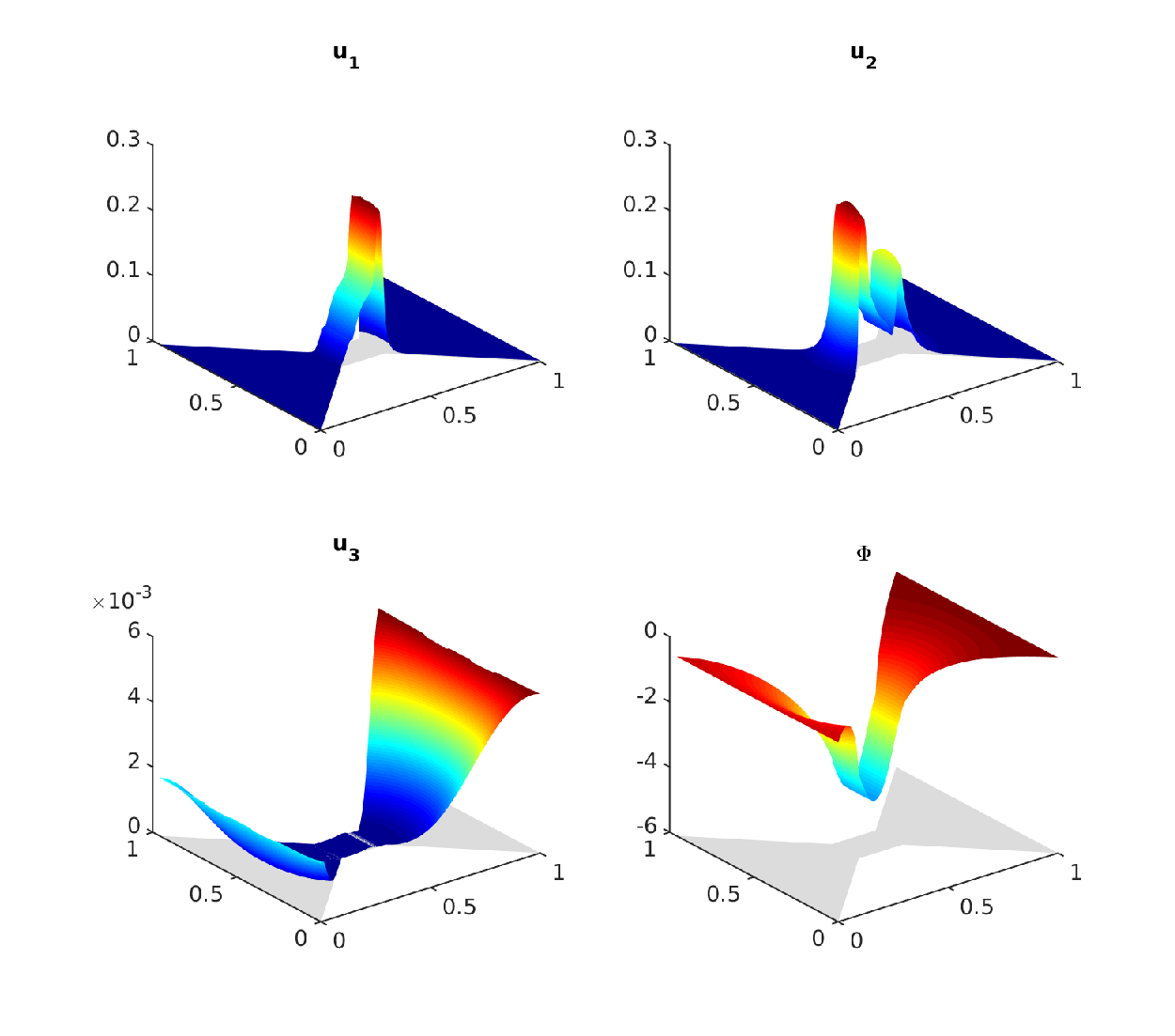
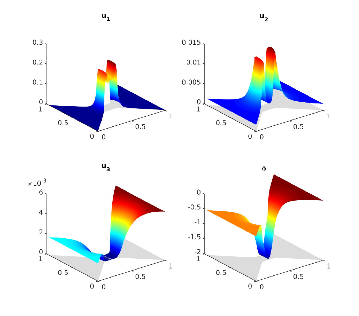
Refer to caption
Figure 2. Scaled concentrations of calcium, sodium, and chloride ions and electric potential after 50 time steps.
Refer to caption
Figure 3. Scaled concentrations of calcium, sodium, and chloride ions and electric potential after 1400 time steps (close to equilibrium).

The simulations suggest that the solution tends towards a steady state as t→∞t\to\infty. The large-time behavior can be quantified by computing the relative entropy EkE^{k} with respect to the stationary solution, where

Ek=∑K∈𝒯m⁡(K)​∑i=0nui,Kk​log⁡(ui,Kkui,K∞)+λ22​∑σ∈ℰτσ​DK,σ​(Φk−Φ∞)2E^{k}=\sum_{K\in{\mathcal{T}}}\mathrm{m}(K)\sum_{i=0}^{n}u_{i,K}^{k}\log\bigg(\frac{u_{i,K}^{k}}{u_{i,K}^{\infty}}\bigg)+\frac{\lambda^{2}}{2}\sum_{\sigma\in{\mathcal{E}}}\tau_{\sigma}\textrm{D}_{K,\sigma}(\Phi^{k}-\Phi^{\infty})^{2}

and (ui,K∞,Φ∞)(u^{\infty}_{i,K},\Phi^{\infty}) is the constant steady state determined from the boundary data. Figure 4 shows that the relative entropy as well as the discrete L1L^{1} norms of the concentrations and electric potential decay with exponential rate. Interestingly, after some initial phase, the convergence is rather slow and increases after this intermediate phase. This phase can be explained by the degeneracy at u0=0u_{0}=0, which causes a small entropy production slowing down diffusion. Indeed, as shown in [20] for the one-dimensional setting, a small change in the oxygen concentration may prolong the intermediate phase of slow convergence drastically.
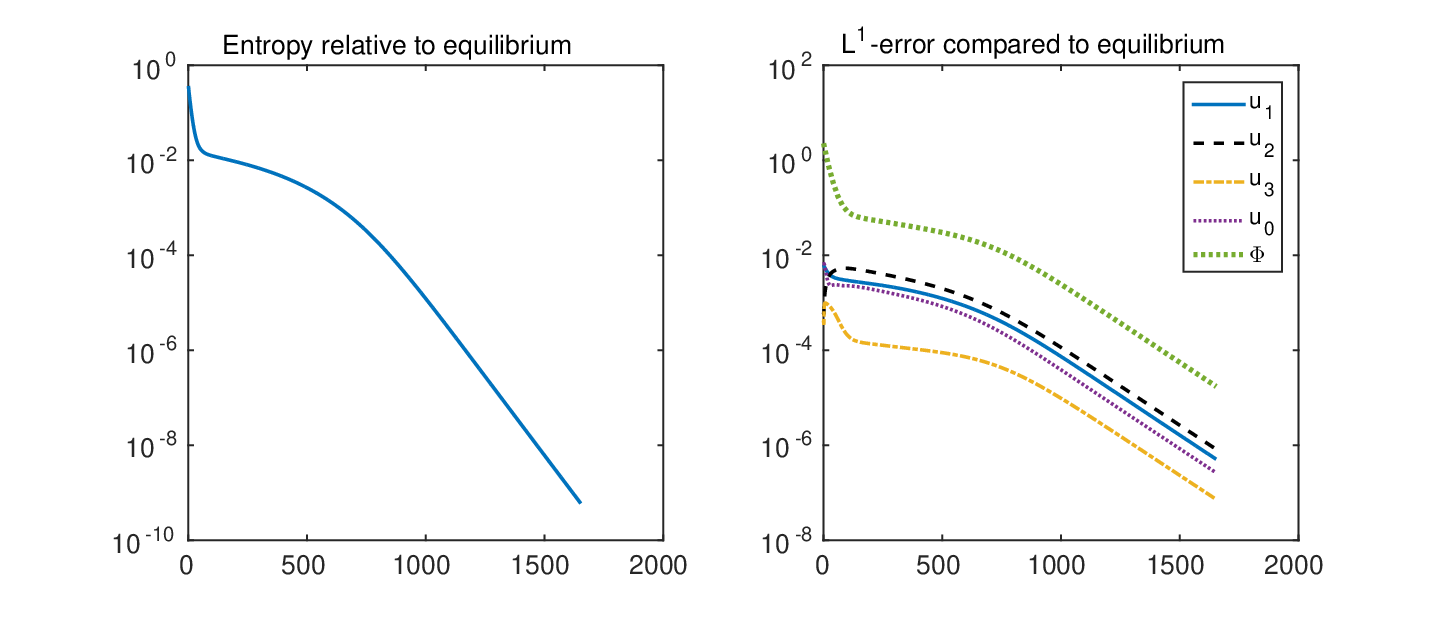
Refer to caption
Figure 4. Relative entropy (left) and discrete L1L^{1} error relative to the equilibrium (right) over the number of time steps.

Since Assumptions (A1)-(A3) are not satisfied in our test case, the convergence result of Theorem 3 cannot be applied here. However, we still observe convergence of the numerical solutions. As the exact solution is not known explicitly, we compute a reference solution on a very fine mesh with 75 776 elements and mesh size h⁡(𝒯)≈0.01h({\mathcal{T}})\approx 0.01. This mesh is obtained from the coarse mesh by a regular refinement, dividing the triangles into four triangles of the same shape. The reference solution is compared to approximate solutions on coarser nested meshes. In Figure 5, the errors in the discrete L1L^{1} norm between the reference solution and the solutions on the coarser meshes at two fixed time steps k=50k=50 and k=1400k=1400 are plotted. We clearly observe the expected first-order convergence in space.

Refer to caption
Figure 5. Discrete L1L^{1} error relative to the reference solution at two different time steps over the mesh size h⁡(𝒯)h({\mathcal{T}}).

Appendix A Auxiliary results

We prove two versions of discrete Aubin-Lions lemmas. The first one is a consequence of [19, Theorem 3.4], the second one extends Lemma 13 in [22] to the discrete case. The latter result is new. Recall that ΩT=Ω×(0,T)\Omega_{T}=\Omega\times(0,T), ∇m=∇𝒯m,△​tm\nabla_{m}=\nabla_{{\mathcal{T}}_{m},{\triangle t}_{m}} is the discrete gradient defined in (39), and ∂t△​t\partial_{t}^{\triangle t} is the discrete time derivative defined in (36).

Lemma 9 (Discrete Aubin-Lions).

Let ∥⋅∥1,𝒯m\|\cdot\|_{1,{\mathcal{T}}_{m}} be the norm on ℋ𝒯m\mathcal{H}_{{\mathcal{T}}_{m}} defined in (11) with the dual norm ∥⋅∥−1,𝒯m\|\cdot\|_{-1,{\mathcal{T}}_{m}} given by (12), and let (um)⊂ℋ𝒯m,△​tm(u_{m})\subset\mathcal{H}_{{\mathcal{T}}_{m},{\triangle t}_{m}} be a sequence of piecewise constants in time functions with values in ℋ𝒯m\mathcal{H}_{{\mathcal{T}}_{m}} satisfying

∑k=1Nm△​t​(‖umk‖1,𝒯m2+‖∂t△​tmumk‖−1,𝒯m2)≤C,\sum_{k=1}^{N_{m}}{\triangle t}\big(\|u_{m}^{k}\|_{1,{\mathcal{T}}_{m}}^{2}+\|\partial_{t}^{{\triangle t}_{m}}u_{m}^{k}\|_{-1,{\mathcal{T}}_{m}}^{2}\big)\leq C,

where C>0C>0 is independent of the size of the mesh and the time step size. Then there exists a subsequence, which is not relabeled, such that, as m→∞m\to\infty,

um→u\displaystyle u_{m}\to u strongly in ​L2​(ΩT),\displaystyle\quad\mbox{strongly in }L^{2}(\Omega_{T}),
∇mum⇀∇u\displaystyle\nabla_{m}u_{m}\rightharpoonup\nabla u weakly in ​L2​(ΩT).\displaystyle\quad\mbox{weakly in }L^{2}(\Omega_{T}).
Proof.

The result is a consequence of Theorem 3.4 in [19]. To apply this theorem, we have to show that the discrete norms ∥⋅∥1,𝒯m\|\cdot\|_{1,{\mathcal{T}}_{m}} and ∥⋅∥−1,𝒯m\|\cdot\|_{-1,{\mathcal{T}}_{m}} satisfy the assumptions of Lemma 3.1 in [19]:

  1. (1)

    For any sequence (vm)⊂ℋ𝒯m(v_{m})\subset\mathcal{H}_{{\mathcal{T}}_{m}} such that there exists C>0C>0 with ‖vm‖1,𝒯m≤C\|v_{m}\|_{1,{\mathcal{T}}_{m}}\leq C for all m∈ℕm\in{\mathbb{N}}, there exists v∈L2​(Ω)v\in L^{2}(\Omega) such that, up to a subsequence, vm→vv_{m}\to v in L2​(Ω)L^{2}(\Omega).

  2. (2)

    If vm→vv_{m}\to v strongly in L2​(Ω)L^{2}(\Omega) and ‖vm‖−1,𝒯m→0\|v_{m}\|_{-1,{\mathcal{T}}_{m}}\to 0 as m→∞m\to\infty, then v=0v=0.

The first property is proved in, for instance, [17, Lemma 5.6]. Here, we need assumption (10) on the mesh. The second property can be replaced, according to [19, Remark 6], by the condition that ∥⋅∥1,𝒯m\|\cdot\|_{1,{\mathcal{T}}_{m}} and ∥⋅∥−1,𝒯m\|\cdot\|_{-1,{\mathcal{T}}_{m}} are dual norms with respect to the L2​(Ω)L^{2}(\Omega) norm, which is the case here. We infer that there exists a subsequence of (um)(u_{m}), which is not relabeled, such that um→uu_{m}\to u strongly in L2​(ΩT)L^{2}(\Omega_{T}). The weak convergence of the discrete gradients can be proved as in Lemma 4.4 in [12]. Indeed, the boundedness of (∇mum)(\nabla_{m}u_{m}) in L2L^{2} implies the convergence to some function χ∈L2​(ΩT)\chi\in L^{2}(\Omega_{T}) (up to a subsequence). In order to show that χ=∇u\chi=\nabla u, it remains to verify that for all test functions ϕ∈C0∞​(ΩT,ℝd)\phi\in C_{0}^{\infty}(\Omega_{T};{\mathbb{R}}^{d}),

∫0T∫Ω∇mum⋅ϕ​𝑑x​𝑑t+∫0T∫Ωum​div​ϕ​𝑑x​𝑑t→0as ​m→∞.\int_{0}^{T}\int_{\Omega}\nabla_{m}u_{m}\cdot\phi dxdt+\int_{0}^{T}\int_{\Omega}u_{m}\operatorname{div}\phi dxdt\to 0\quad\mbox{as }m\to\infty.

This limit follows from the definition of ∇mum\nabla_{m}u_{m} and the regularity of the mesh. We refer to [12, Lemma 4.4] for details. ∎

Lemma 10 (Discrete Aubin-Lions of “degenerate” type).

Let (ym)(y_{m}) and (zm)(z_{m}) be sequences in ℋ𝒯m,△​tm\mathcal{H}_{{\mathcal{T}}_{m},{\triangle t}_{m}} which are bounded in L∞​(ΩT)L^{\infty}(\Omega_{T}) and let (ym)(y_{m}) be relatively compact in L2​(ΩT)L^{2}(\Omega_{T}), i.e., up to a subsequence, ym→yy_{m}\to y strongly in L2​(ΩT)L^{2}(\Omega_{T}) and zm⇀∗zz_{m}\rightharpoonup^{*}z weakly* in L∞​(ΩT)L^{\infty}(\Omega_{T}). Furthermore, suppose that, for some constant C>0C>0 independent of mm,

∑k=1Nm△​tm​(‖ymk‖1,𝒯m2+‖ymk​zmk‖1,𝒯m2+‖∂t△​tmzmk‖−1,𝒯m2)≤C.\sum_{k=1}^{N_{m}}{\triangle t}_{m}\big(\|y_{m}^{k}\|_{1,{\mathcal{T}}_{m}}^{2}+\|y_{m}^{k}z_{m}^{k}\|_{1,{\mathcal{T}}_{m}}^{2}+\|\partial_{t}^{{\triangle t}_{m}}z_{m}^{k}\|_{-1,{\mathcal{T}}_{m}}^{2}\big)\leq C.

Then there exists a subsequence which is not relabeled such that ym​zm→y​zy_{m}z_{m}\to yz strongly in L2​(ΩT)L^{2}(\Omega_{T}) as m→∞m\to\infty.

Proof.

The idea of the proof is to use the Kolmogorov-Riesz theorem [9, Theorem 4.26] as in the continuous case; see [10, Section 4.4] or [22, Lemma 13]. The discrete case, however, makes necessary some changes in the calculations. We need to show that

(48) lim(ξ,τ)→0∫0T−τ∫ω((ym​zm)​(x+ξ,t+τ)−(ym​zm)​(x,t))2​𝑑x​𝑑t=0\lim_{(\xi,\tau)\to 0}\int_{0}^{T-\tau}\int_{\omega}\big((y_{m}z_{m})(x+\xi,t+\tau)-(y_{m}z_{m})(x,t)\big)^{2}dxdt=0

uniformly in mm, where ω⊂Ω\omega\subset\Omega satisfies x+ξ∈Ωx+\xi\in\Omega for all x∈ωx\in\omega. First, we separate the space and time translation:

∫0T−τ∫ω\displaystyle\int_{0}^{T-\tau}\int_{\omega} ((ym​zm)​(x+ξ,t+τ)−(ym​zm)​(x,t))2​d​x​d​t\displaystyle\Big((y_{m}z_{m})(x+\xi,t+\tau)-(y_{m}z_{m})(x,t)\Big)^{2}dxdt
≤2​∫0T−τ∫ω((ym​zm)​(x+ξ,t+τ)−(ym​zm)​(x,t+τ))2​𝑑x​𝑑t\displaystyle\leq 2\int_{0}^{T-\tau}\int_{\omega}\Big((y_{m}z_{m})(x+\xi,t+\tau)-(y_{m}z_{m})(x,t+\tau)\Big)^{2}dxdt
+2∫0T−τ∫ω((ymzm)(x,t+τ)−(ymzm)(x,t))2dxdt=:I1+I2.\displaystyle\phantom{xx}{}+2\int_{0}^{T-\tau}\int_{\omega}\Big((y_{m}z_{m})(x,t+\tau)-(y_{m}z_{m})(x,t)\Big)^{2}dxdt=:I_{1}+I_{2}.

For the estimate of I1I_{1}, we apply a result for space translations of piecewise constant functions vv with uniform bounds in the discrete H1​(Ω)H^{1}(\Omega) norm, namely

∥v(⋅+ξ)−v∥L2​(Ω)2≤|ξ|(|ξ|+Ch(𝒯))∥v∥1,𝒯2\|v(\cdot+\xi)-v\|_{L^{2}(\Omega)}^{2}\leq|\xi|\big(|\xi|+Ch({\mathcal{T}})\big)\|v\|_{1,{\mathcal{T}}}^{2}

for appropriate ξ\xi, where C>0C>0 only depends on Ω\Omega [15, Lemma 4]. This shows that

I1≤C1​|ξ|​(|ξ|+C​h​(𝒯m))I_{1}\leq C_{1}|\xi|\big(|\xi|+Ch({\mathcal{T}}_{m})\big)

converges to zero as ξ→0\xi\to 0 uniformly in mm.

For the second integral I2I_{2}, we write

I2\displaystyle I_{2} ≤4​∫0T−τ∫ωzm​(x,t+τ)2​(ym​(x,t+τ)−ym​(x,t))2​𝑑x​𝑑t\displaystyle\leq 4\int_{0}^{T-\tau}\int_{\omega}z_{m}(x,t+\tau)^{2}\big(y_{m}(x,t+\tau)-y_{m}(x,t)\big)^{2}dxdt
+4∫0T−τ∫ωym(x,t)2(zm(x,t+τ)−zm(x,t))2dxdt=:I21+I22.\displaystyle\phantom{xx}{}+4\int_{0}^{T-\tau}\int_{\omega}y_{m}(x,t)^{2}\big(z_{m}(x,t+\tau)-z_{m}(x,t)\big)^{2}dxdt=:I_{21}+I_{22}.

The L∞L^{\infty} bounds on zmz_{m} give

I21≤C​∫0T−τ∫ω(ym​(x,t+τ)−ym​(x,t))2​𝑑x​𝑑t.I_{21}\leq C\int_{0}^{T-\tau}\int_{\omega}\big(y_{m}(x,t+\tau)-y_{m}(x,t)\big)^{2}dxdt.

By assumption, the sequence (ym)(y_{m}) is relatively compact in L2​(ΩT)L^{2}(\Omega_{T}). Therefore, we can apply the inverse of the Kolmogorov-Riesz theorem [9, Exercise 4.34] to conclude that I21I_{21} converges to zero as τ→0\tau\to 0 uniformly in mm.

The analysis of I22I_{22} is more involved. We split the integral in several parts:

I22\displaystyle I_{22} =∫0T−τ∫ωym​(x,t)2​zm​(x,t)​(zm​(x,t)−zm​(x,t+τ))​𝑑x​𝑑t\displaystyle=\int_{0}^{T-\tau}\int_{\omega}y_{m}(x,t)^{2}z_{m}(x,t)\big(z_{m}(x,t)-z_{m}(x,t+\tau)\big)dxdt
+∫0T−τ∫ωym(x,t+τ)2zm(x,t+τ)(zm(x,t+τ)−zm(x,t))dxdt\displaystyle\phantom{xx}{}+\int_{0}^{T-\tau}\int_{\omega}y_{m}(x,t+\tau)^{2}z_{m}(x,t+\tau)\big(z_{m}(x,t+\tau)-z_{m}(x,t)\big)dxdt
+∫0T−τ∫ω(ym(x,t)2−ym(x,t+τ)2)zm(x,t+τ)(zm(x,t+τ)−zm(x,t))dxdt\displaystyle\phantom{xx}{}+\int_{0}^{T-\tau}\int_{\omega}\big(y_{m}(x,t)^{2}-y_{m}(x,t+\tau)^{2}\big)z_{m}(x,t+\tau)\big(z_{m}(x,t+\tau)-z_{m}(x,t)\big)dxdt
=:J1+J2+J3.\displaystyle=:J_{1}+J_{2}+J_{3}.

The first two integrals J1J_{1} and J2J_{2} are treated similarly as in [8, Lemma 3.11]. Indeed, let ⌈s⌉\lceil s\rceil denote the smallest integer larger or equal to ss. Defining nm​(t):=⌈t/△​tm⌉n_{m}(t):=\lceil t/{\triangle t}_{m}\rceil, we can formulate

zm​(x,t+τ)−zm​(x,t)=∑k=nm​(t)+1nm​(t+τ)(zm,Kk−zm,Kk−1)z_{m}(x,t+\tau)-z_{m}(x,t)=\sum_{k=n_{m}(t)+1}^{n_{m}(t+\tau)}\big(z^{k}_{m,K}-z^{k-1}_{m,K}\big)

for x∈Kx\in K, 0≤t≤T−τ0\leq t\leq T-\tau. With this formulation, we can bound J1J_{1}, using the duality of ∥⋅∥1,𝒯m\|\cdot\|_{1,{\mathcal{T}}_{m}} and ∥⋅∥−1,𝒯m\|\cdot\|_{-1,{\mathcal{T}}_{m}}:

J1\displaystyle J_{1} ≤∫0T−τ(∑K∈𝒯mm⁡(K)​(ym,Knm​(t))2​zm,Knm​(t)​∑k=nm​(t)+1nm​(t+τ)(zm,Kk−1−zm,Kk))​𝑑t\displaystyle\leq\int_{0}^{T-\tau}\bigg(\sum_{K\in{\mathcal{T}}_{m}}\mathrm{m}(K)\big(y_{m,K}^{n_{m}(t)}\big)^{2}z_{m,K}^{n_{m}(t)}\sum_{k=n_{m}(t)+1}^{n_{m}(t+\tau)}\big(z^{k-1}_{m,K}-z^{k}_{m,K}\big)\bigg)dt
≤∫0T−τ(∑k=nm​(t)+1nm​(t+τ)‖(ymnm​(t))2​zmnm​(t)‖1,𝒯m​‖zmk−zmk−1‖−1,𝒯m)​𝑑t\displaystyle\leq\int_{0}^{T-\tau}\bigg(\sum_{k=n_{m}(t)+1}^{n_{m}(t+\tau)}\big\|(y_{m}^{n_{m}(t)})^{2}z_{m}^{n_{m}(t)}\big\|_{1,{\mathcal{T}}_{m}}\big\|z^{k}_{m}-z^{k-1}_{m}\big\|_{-1,{\mathcal{T}}_{m}}\bigg)dt
≤12​∫0T−τ∑k=nm​(t)+1nm​(t+τ)△​tm​‖(ymnm​(t))2​zmnm​(t)‖1,𝒯m2​𝑑t\displaystyle\leq\frac{1}{2}\int_{0}^{T-\tau}\sum_{k=n_{m}(t)+1}^{n_{m}(t+\tau)}{\triangle t}_{m}\|(y_{m}^{n_{m}(t)})^{2}z_{m}^{n_{m}(t)}\|_{1,{\mathcal{T}}_{m}}^{2}dt
+12∫0T−τ∑k=nm​(t)+1nm​(t+τ)1△​tm∥zkm−zk−1m∥−1,𝒯m2dt\displaystyle\phantom{xx}{}+\frac{1}{2}\int_{0}^{T-\tau}\sum_{k=n_{m}(t)+1}^{n_{m}(t+\tau)}\frac{1}{{\triangle t}_{m}}\big\|z^{k}_{m}-z^{k-1}_{m}\big\|_{-1,{\mathcal{T}}_{m}}^{2}dt
≤τ2​∑k=1Nm△​tm​‖(ymk)2​zmk‖1,𝒯m2+τ2​∑k=1Nm1△​tm​‖zmk−zmk−1‖−1,𝒯m2,\displaystyle\leq\frac{\tau}{2}\sum_{k=1}^{N_{m}}{\triangle t}_{m}\|(y_{m}^{k})^{2}z_{m}^{k}\|_{1,{\mathcal{T}}_{m}}^{2}+\frac{\tau}{2}\sum_{k=1}^{N_{m}}\frac{1}{{\triangle t}_{m}}\big\|z^{k}_{m}-z^{k-1}_{m}\big\|_{-1,{\mathcal{T}}_{m}}^{2},

where the last inequality follows from [5, Lemmas 4.1 and 4.2]. Let us remark that, for all σ=K|L∈ℰint\sigma=K|L\in{\mathcal{E}}_{\rm int}, we can rewrite

(yK)2​zK−(yL)2​zL=yK+yL2​(yK​zK−yL​zL)+yK​zK+yL​zL2​(yK−yL).(y_{K})^{2}z_{K}-(y_{L})^{2}z_{L}=\frac{y_{K}+y_{L}}{2}(y_{K}z_{K}-y_{L}z_{L})+\frac{y_{K}z_{K}+y_{L}z_{L}}{2}(y_{K}-y_{L}).

Then,

‖(ymk)2​zmk‖1,𝒯m2≤m⁡(Ω)​‖(ymk)2​zmk‖L∞​(Ω)2+‖ymk‖L∞​(Ω)​‖ymk​zmk‖1,𝒯m+‖ymk​zmk‖L∞​(Ω)​‖ymk‖1,𝒯m.\|(y_{m}^{k})^{2}z_{m}^{k}\|_{1,{\mathcal{T}}_{m}}^{2}\leq\mathrm{m}(\Omega)\|(y_{m}^{k})^{2}z_{m}^{k}\|_{L^{\infty}(\Omega)}^{2}+\|y_{m}^{k}\|_{L^{\infty}(\Omega)}\|y_{m}^{k}z_{m}^{k}\|_{1,{\mathcal{T}}_{m}}+\|y_{m}^{k}z_{m}^{k}\|_{L^{\infty}(\Omega)}\|y_{m}^{k}\|_{1,{\mathcal{T}}_{m}}.

Hence, J1≤C​τJ_{1}\leq C\tau for some C>0C>0. An analogous estimation leads to J2≤C​τJ_{2}\leq C\tau. It remains to estimate the integral J3J_{3}. For this, we use, similar to the treatment of I21I_{21}, the L∞L^{\infty} bounds on ymy_{m} and zmz_{m}:

J3≤C​∫0T−τ∫ω|ym​(x,t+τ)−ym​(x,t)|​𝑑x​𝑑t.J_{3}\leq C\int_{0}^{T-\tau}\int_{\omega}\big|y_{m}(x,t+\tau)-y_{m}(x,t)\big|dxdt.

This expression converges to zero uniformly in mm because of the relative compactness of (ym)(y_{m}) in L2​(ΩT)L^{2}(\Omega_{T}).

We deduce from the previous computations that (48) holds true. Therefore, the product (ym​zm)(y_{m}z_{m}) converges strongly in L2​(ΩT)L^{2}(\Omega_{T}), up to some subsequence, and in view of the convergences ym→yy_{m}\to y strongly in L2​(ΩT)L^{2}(\Omega_{T}) and zm⇀∗zz_{m}\rightharpoonup^{*}z weakly* in L∞​(0,T,L∞​(Ω))L^{\infty}(0,T;L^{\infty}(\Omega)), the limit of (ym​zm)(y_{m}z_{m}) equals y​zyz, which finishes the proof. ∎

References

  • [1] A. Ait Hammou Oulhaj. Numerical analysis of a finite volume scheme for a seawater intrusion model with cross-diffusion in an unconfined aquifer. Numer. Meth. Partial Diff. Eqs., Online First, 2017. DOI:10.1002/num.22234.
  • [2] V. Anaya, M. Bendahmane, M. Langlais, and M. Sepúlveda. A convergent finite volume method for a model of indirectly transmitted diseases with nonlocal cross-diffusion. Comput. Math. Appl. 70 (2015), 132-157.
  • [3] V. Anaya, M. Bendahmane, and M. Sepúlveda. Numerical analysis for a three interacting species model with nonlocal and cross diffusion. ESAIM Math. Model. Numer. Anal. 49 (2015), 171-192.
  • [4] B. Andreianov, M. Bendahmane, and R. R. Baier. Analysis of a finite volume method for a cross-diffusion model in population dynamics. Math. Models Meth. Appl. Sci. 21 (2011), 307-344.
  • [5] O. Angelini, K. Brenner, and D. Hilhorst. A finite volume method on general meshes for a degenerate parabolic convection-reaction-diffusion equation. Numer. Math. 123 (2013), 219-257.
  • [6] M. Bessemoulin-Chatard, C. Chainais-Hillairet, and F. Filbet. On discrete functional inequalities for some finite volume schemes. IMA J. Numer. Anal. 35 (2015), 1125-1149.
  • [7] M. Bessemoulin-Chatard, and A. Jüngel. A finite volume scheme for a Keller-Segel model with additional cross-diffusion. IMA J. Numer. Anal. 34 (2014), 96-122.
  • [8] K. Brenner, and R. Masson. Convergence of a vertex centred discretization of two-phase Darcy flows on general meshes. Intern. J. Finite Vol. 10 (2013), 1-37.
  • [9] H. Brézis. Functional Analysis, Sobolev Spaces and Partial Differential Equations. Springer, New York, 2011.
  • [10] M. Burger, M. Di Francesco, J.-F. Pietschmann, and B. Schlake. Nonlinear cross-diffusion with size exclusion. SIAM J. Math. Anal. 42 (2010), 2842-2871.
  • [11] M. Burger, B. Schlake, and M.-T. Wolfram. Nonlinear Poisson-Nernst-Planck equations for ion flux through confined geometries. Nonlinearity 25 (2012), 961-990.
  • [12] C. Chainais-Hillairet, J.-G. Liu, and Y.-J. Peng. Finite volume scheme for multi-dimensional drift-diffusion equations and convergence analysis. ESAIM Math. Model. Numer. Anal. 37 (2003), 319-338.
  • [13] K. Deimling. Nonlinear functional analysis. Springer, Berlin, 1985.
  • [14] R. Eymard, T. Gallouët, M. Ghilani and R. Herbin. Error estimates for the approximate solutions of a nonlinear hyperbolic equation given by finite volume schemes. IMA J. Numer. Anal. 18 (1998), 563-594.
  • [15] R. Eymard, T. Gallouët, and R. Herbin. Convergence of finite volume schemes for semilinear convection diffusion equations. Numer. Math. 82 (1999), 91-116.
  • [16] R. Eymard, T. Gallouët, and R. Herbin. Finite volume methods. In: P. G. Ciarlet and J.-L. Lions (eds.), Handbook of Numerical Analysis 7 (2000), 713-1018.
  • [17] R. Eymard, T. Gallouët, and R. Herbin. Finite volume methods. Schemes and Analysis. Course at the University of Wroclaw. Lecture notes, 2008. Available at
    http://www.math.uni.wroc.pl/~olech/courses/skrypt_Roberta_wroclaw.pdf.
  • [18] H. Gajewski. On a variant of monotonicity and its application to differential equations. Nonlin. Anal. TMA 22 (1994), 73-80.
  • [19] T. Gallouët and J.-C. Latché. Compactness of discrete approximate solutions to parabolic PDEs – Application to a turbulence model. Commun. Pure Appl. Anal. 11 (2012), 2371-2391.
  • [20] A. Gerstenmayer, and A. Jüngel. Analysis of a degenerate parabolic cross-diffusion system for ion transport. To appear in J. Math. Anal. Appl., 2018. arXiv:1706.07261.
  • [21] D. Gillespie, W. Nonner, and R. Eisenberg. Coupling Poisson-Nernst-Planck and density functional theory to calculate ion flux. J. Phys.: Condens. Matter 14 (2002), 12129-12145.
  • [22] A. Jüngel. The boundedness-by-entropy method for cross-diffusion systems. Nonlinearity 28 (2015), 1963-2001.
  • [23] A. Jüngel. Entropy Methods for Diffusive Partial Differential Equations. BCAM Springer Briefs, Springer, 2016.
  • [24] H. Murakawa. A linear finite volume method for nonlinear cross-diffusion systems. Numer. Math. 136 (2017), 1-26.
  • [25] W. Nernst. Zur Kinetik der in Lösung befindlichen Körper. Z. Phys. Chem. 2 (1888), 613-637.
  • [26] K. Rahman and H. Eberl. Numerical treatment of a cross-diffusion model of biofilm exposure to antimicrobials. In: R.  Wyrzykowski, J. Dongarra, K. Karczewski, and J. Waśniewski (eds.), Parallel Processing and Applied Mathematics. Part I, 134-–144, Lect. Notes Comput. Sci. 8384, Springer, Heidelberg, 2014.
  • [27] M. Simpson, K. Landman, and B. Hughes. Multi-species simple exclusion processes. Phys. A 388 (2009), 399-406.
  • [28] N. Zamponi and A. Jüngel. Analysis of degenerate cross-diffusion population models with volume filling. Ann. I. H. Poincaré – Anal. Non Lin. 34 (2017), 1-29. (Erratum: 34 (2017), 789-792.)