Trefftz Approximations in Complex Media:
Accuracy and Applications
Abstract
Approximations by Trefftz functions are rapidly gaining popularity in the numerical solution of boundary value problems of mathematical physics. By definition, these functions satisfy locally, in weak form, the underlying differential equations of the problem, which often results in high-order or even exponential accuracy with respect to the size of the basis set. We highlight two separate examples in applied electromagnetics and photonics: (i) homogenization of periodic structures, and (ii) numerical simulation of electromagnetic waves in slab geometries. Extensive numerical evidence and theoretical considerations show that Trefftz approximations can be applied much more broadly than is traditionally done: they are effective not only in physically homogeneous regions but also in complex inhomogeneous ones. Two mechanisms underlying the high accuracy of Trefftz approximations in such complex cases are pointed out. The first one is related to trigonometric interpolation and the second one – somewhat surprisingly – to well-posedness of random matrices.
Keywords:
Trefftz approximations , convergence , Maxwell’s equations , homogenization , photonic devices , wave scattering , interpolation , finite difference schemes , random matrices2010 MSC
65M06 , 76M20 , 35B27 , 76M50 , 74Q15 , 35Q61 , 15B521 Introduction
Many classical numerical methods for partial differential equations rely on polynomial or piecewise-polynomial approximations of the solution. Examples include traditional finite difference (FD) schemes, the finite element method (FEM), and the boundary element method (BEM). But a strong incentive to achieve qualitatively higher accuracy of the numerical solution has led, over several decades of research, to the development of Trefftz-based methods. By definition, Trefftz functions satisfy locally (in weak form) the underlying differential equations of the problem, which often results in high-order algebraic or even exponential convergence with respect to the dimension of the basis. This qualitative accuracy improvement has been demonstrated in a large variety of mathematical methods and engineering applications: Domain Decomposition [1, 2], Generalized FEM [3, 4, 5, 6, 7, 8], Discontinuous Galerkin [2, 9, 10, 11, 12, 13, 14, 15], and finite difference (“Flexible Local Approximation MEthods,” FLAME) [16, 17, 18, 19].
It is not our intention to review all, or even some, of these Trefftz-oriented methods; several good reviews are already available: [20, 21] and especially [22]. Rather, our focus is on one question central in these methods: why are Trefftz approximations so effective?
A simplified intuitive picture is shown in Fig. 1, left panel. Several incident waves, schematically indicated with solid arrows, are impinging on an object (in general, physically inhomogeneous) and give rise to the respective total fields inside and to scattered fields outside that object. For visual clarity, only the incident waves are sketched in the figure, and their number is limited to three.
The total fields inside the scatterer, by definition, form a Trefftz set. One may view it as a “database” or “training set,” which can be precomputed and then used to approximate the field induced by another wave, indicated with a dashed arrow and a question mark in Fig. 1. This approximation of one physically meaningful solution by other physically meaningful solutions (as opposed to, say, generic polynomials) certainly makes intuitive sense but is not trivial from the mathematical perspective.

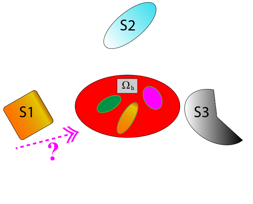
The right panel of Fig. 1 illustrates a more interesting, and more complicated, case. Suppose that the Trefftz training set has been generated for the original inhomogeneous scatterer – same as in the left panel. However, the unknown “dashed arrow” solution may involve additional objects – such as S1, S2, S3 – in the computational domain. Obviously, under this complication, little can be inferred about the unknown solution from the Trefftz set in the whole domain, especially in the regions around the additional scatterers. One may hope, however, that the field within a given small subdomain inside the original scatterer can still be approximated accurately as a superposition of the known Trefftz waves. This setup is the central issue of Sections 6.2, 6.3, and is inspired by our numerical experiments with pseudorandom structures of Section 5, as well as by our earlier work on multiparticle problems [23].
The overall motivation for the paper is to highlight applications of Trefftz functions to problems involving complex, inhomogeneous media. Much of mathematical analysis so far has revolved around the homogeneous case (that is, equations with constant coefficients), where cylindrical, spherical or plane waves serve as Trefftz functions for the Helmholtz equation, while harmonic polynomials are used for the Laplace equation. One can refer, for example, to papers by Melenk, Hiptmair, Moiola, Perugia et al. cited above, to the references in these papers, and to Perrey-Debain’s paper [24]. Much less attention has been paid to the inhomogeneous case [25, Chapter IV], [26, Section 3], [27, 28], which is substantially more complicated but at the same time more rewarding in practice.
For illustration, in Sections 4 and 5 we consider two application examples where Trefftz approximations prove to be effective for two different variations of the generic setup shown in Fig. 1. The first example is non-asymptotic and nonlocal two-scale homogenization. Instead of a single scatterer, in this case one deals with a periodic structure; Trefftz functions on the fine scale are Bloch waves traveling in different directions, and on the coarse scale – the corresponding plane waves.
The second example involves a common setup in metasurface and nanophotonics research: a patterned finite-thickness slab. This problem is especially challenging computationally when the pattern is non-periodic and the slab is geometrically large relative to the vacuum wavelength. One possible simulation procedure relies on high-order Trefftz difference schemes (FLAME). The Trefftz bases are computed “locally,” i.e. over relatively small segments of the structure (Section 5).
2 Preliminaries: Trigonometric Projection and Interpolation
Trigonometric approximation of periodic functions is a well-established subject. Here we summarize the key mathematical results that will be needed in Section 6.1.
For any Lipschitz-continuous periodic function on , one may consider its best possible approximation by a trigonometric polynomial in the maximum norm:
| (1) |
where
| (2) |
A slightly modified notation of [29] is used here. Note that the total number of coefficients , in the trigonometric series is .
It follows from Jackson’s theorem [30], or [29, Theorem 41], that if the derivative exists and is bounded, i.e.
| (3) |
then
| (4) |
For reasons that will become apparent in Section 6.1, we are interested primarily in trigonometric interpolation rather than the best approximation, and thus need to relate the two. The interpolant of a given function over a set of equidistant knots is defined in a standard way, by requiring that
| (5) |
It is known that this interpolant exists and is unique. Furthermore, there is an upper bound for the interpolation error:
| (6) |
where is the Lebesgue constant, which itself has an upper bound [31]
| (7) |
All the above information can be found in a variety of sources, including very recent ones [32, 33], [34, Section 7].
Combining (6), (7), and (4), one has
| (8) |
This indicates fast uniform algebraic convergence of the interpolant with respect to the number of knots. Moreover, under additional assumptions of analyticity of in a strip of the complex plane Re, , convergence becomes exponential [34, (7.19)]:
| (9) |
We are also interested in the approximation of the integral
| (10) |
using the values of at the equispaced knots:
| (11) |
which is the trapezoidal rule for the numerical quadrature. Under the same analyticity assumptions as above, the error of this quadrature can be bounded as [34, (7.20)]
| (12) |
A similar result can be found in [32, Theorem 1]. Adapted to our needs and notation, it states:
If is times continuously differentiable and is Lipschitz continuous, then
| (13) |
If can be analytically continued to a -periodic function for for some , then for any ,
| (14) |
The qualitative conclusion of this section is that trigonometric interpolation of a smooth periodic function provides a very accurate approximation of the function and its integrals.
3 Preliminaries: Finite Difference Trefftz Schemes
Another preliminary subject, which will be needed in Section 5, is FLAME [16, 17, 18, 19, 35, 36]. Recall that classical FD schemes are typically derived from Taylor expansions; but this is problematic if the solution is not sufficiently smooth – e.g. at material interfaces. That is the root cause of the notorious “staircase” effect at slanted or curved interface boundaries that do not conform geometrically to the grid lines. FLAME replaces Taylor polynomials with Trefftz functions, which often produces high-order schemes.
The key ideas of FLAME are as follows. Let a boundary value problem be defined in a computational domain and consider a small subdomain within which a difference scheme is to be formed. In , introduce a set of degrees of freedom (DoF). These DoF are, by definition, linear functionals, (), each mapping any admissible field to a number (real or complex, depending on the problem). The simplest example of DoF for a scalar field is as set of nodal values , where are a set of grid nodes in . In the case of vector fields, one may also consider fluxes, circulations, etc. as other examples of DoF .
Locally, within , the solution is approximated by a linear combination of Trefftz functions () :
| (15) |
where is a coefficient vector and is a vector of basis functions (both generally complex). In , we seek an FD equation of the form
| (16) |
where is a vector of complex coefficients (a “scheme”) to be determined. In the simplest version of FLAME, the scheme is required to be exact for any linear combination (15) of basis functions. Then, after straightforward algebra, one obtains [17, 18]
| (17) |
There are also least-squares versions of this idea [37, 16].
Many illustrative examples are given in [35, 17, 18]. Here we mention just one of them, closely related to the construction of FLAME schemes in Section 5. For the 2D Helmholtz equation, one may consider a Trefftz basis set of eight plane waves traveling at the angles (), where is a given angle; practical choices are or . Evaluating these plane waves over a standard grid “molecule,” one obtains an matrix whose null vector is the FLAME scheme. The result for is a nine-point () order-six scheme [18]. For , one arrives at a scheme derived by Babuška et al. in 1995 [38] from very different considerations.
4 Trefftz Homogenization of Electromagnetic Structures
We consider Trefftz-based homogenization of electromagnetic periodic structures (photonic crystals and metamaterials). The general description of the problem in this section follows [39, 40] closely; but our focus here is on Trefftz approximation, the importance of other aspects of the problem notwithstanding.
The physical essence of the problem is as follows. A sample of a periodic material is illuminated by incoming monochromatic electromagnetic waves at a given frequency and the corresponding free-space wavenumber . To sidestep the complicated problem of field behavior at corners, the sample is assumed to be a finite-thickness slab contained between the planes and , and infinite in the and directions. The periodic medium in the sample is to be replaced with a homogeneous material in such a way that the scattering wave pattern would be preserved as accurately as possible.
Following [39, 40], let us define the problem more precisely. Assume that the intrinsic dielectric permittivity within the slab is lattice-periodic, and that all material constituents are nonmagnetic, . Let all constitutive relationships be local and linear, and let the sample be illuminated by monochromatic waves with a given far-field pattern; these waves are reflected by the metamaterial.
The problem has two principal scales (levels). Fine-level fields are the exact solutions of Maxwell’s equations for given illumination conditions for a given sample. These fields are denoted with small letters , , and . In general, their variation in space is rapid and consistent with the microstructure of metamaterial cells. Coarse-level fields , , , vary on a characteristic scale greater that the cell size. They represent some smoothed (averaged) versions of the fine-level fields and are auxiliary mathematical constructions rather than measurable physical quantities. The coarse-level fields are sought to satisfy Maxwell’s equations and all interface boundary conditions as accurately as possible.
Importantly, effective magnetic properties of metamaterials cannot be determined from the bulk behavior alone as a matter of principle. This is due, in particular, to the fact that the Maxwell equation is invariant with respect to an arbitrary simultaneous rescaling of vectors H and D. Loosely speaking, bulk behavior defines the dispersion relation only, while magnetic characteristics depend on the boundary impedance as well.
The fine-level fields satisfy macroscopic Maxwell’s equations of the form
| (18) |
everywhere in space, supplemented by the usual radiation boundary conditions at infinity. Outside the slab, the most general solution of (18) can be written as a superposition of incident, transmitted and reflected waves. For the electric field, we can write these in the form of angular-spectrum expansions [40]:
| (19a) | |||
| (19b) | |||
| (19c) | |||
where
| (20) |
and the square root branch is defined by the condition . Expressions for the magnetic field are obtained from (19) by using the second Maxwell equation in (18). In (19), , and are the angular spectra of the incident, transmitted and reflected fields. Waves included in these expansions can be evanescent or propagating. For propagating waves, , otherwise the waves are evanescent.
Everywhere in space, the total electric field can be written as a superposition of the incident and scattered fields, viz,
| (21) |
Outside the material, the reflected and transmitted fields form the scattered field:
| (22) |
The scattered field inside the material is also formally defined by (21).
It is natural to approximate fine-level fields via a basis set of Bloch waves traveling in different directions:
| (23) |
where index labels both the wave vector and the polarization state of the Bloch wave in a lattice cell ; , are the respective lattice-periodic factors. As the notation indicates, the basis is defined cell-wise; different bases in different lattice cells could be used. This makes the homogenization problem tractable and reducible to a single cell, rather than global and encompassing the whole sample.
On the coarse scale, a natural counterpart of the fine-scale Bloch basis is a set of generalized plane waves
| (24) |
which satisfy Maxwell’s equations in a homogeneous but possibly anisotropic medium; subscript ‘0’ indicates the field amplitudes to be determined.
Further technical details of the procedure can be found in [40, 39]. The final result is as follows. First, the coarse-level wave vector for each plane wave is taken to be the same as its counterpart for the corresponding Bloch wave, which is already reflected in our notation above (23), (24). Secondly, the amplitudes of each plane wave are the boundary average of the tangential components of the respective fine-scale Bloch wave:
| (25) |
The averaging operator for tangential components of a generic vector field is defined, in the case of an orthorhombic cell , as
| (26) |
Here acts simply as the Kronecker delta for the faces of the cell parallel to a given coordinate direction , . Note that the averages in (25) involve the periodic factor of the Bloch wave. The amplitudes , , along with the Bloch wave vector, define the coarse-level basis function in a lattice cell .
The homogenization procedure of [39, 40] leads to a system of algebraic equations of the form
| (27) |
Here ‘l.s.’ stands for ‘least squares’. Each column of the rectangular matrix corresponds to a given coarse-level basis function , and the entries of that column are the -components of the wave amplitudes , . The number of columns is equal to the chosen number of basis functions; the number of rows is, in general, six, unless some of the field components are known to be zero (e.g. for - or -polarized waves). The matrix is completely analogous and contains the amplitudes derived from Maxwell’s curl equations:
| (28) |
The (local) material tensor is represented, in general, by a matrix. Since the number of columns in matrix is typically greater than the number of rows, the matrix equation (27) for the material tensor is solved in the least squares sense:
| (29) |
where is the Moore-Penrose pseudoinverse of , and is the associated least-squares error.


As demonstrated in [39], the homogenization accuracy can be further improved by including, in addition to the amplitudes, integral DoF of the form
| (30) |
where is a convolution kernel depending only on the coordinates tangential to the boundary of the sample:
A natural (but certainly not unique) choice for this kernel is a Gaussian
where the amplitude and width are adjustable parameters, and is the unit normal vector.
Since our focus is on the approximation properties of Trefftz functions and not on the homogenization procedure per se, we do not discuss the physics of the problem here, or the merits and demerits of nonlocal vs. local theory.11 1 It should, however, be noted that our nonlocal procedure operates in real space, in contrast with -space techniques that we critiqued elsewhere [41]. We also omit further technical details and limit ourselves to just one illustration example.
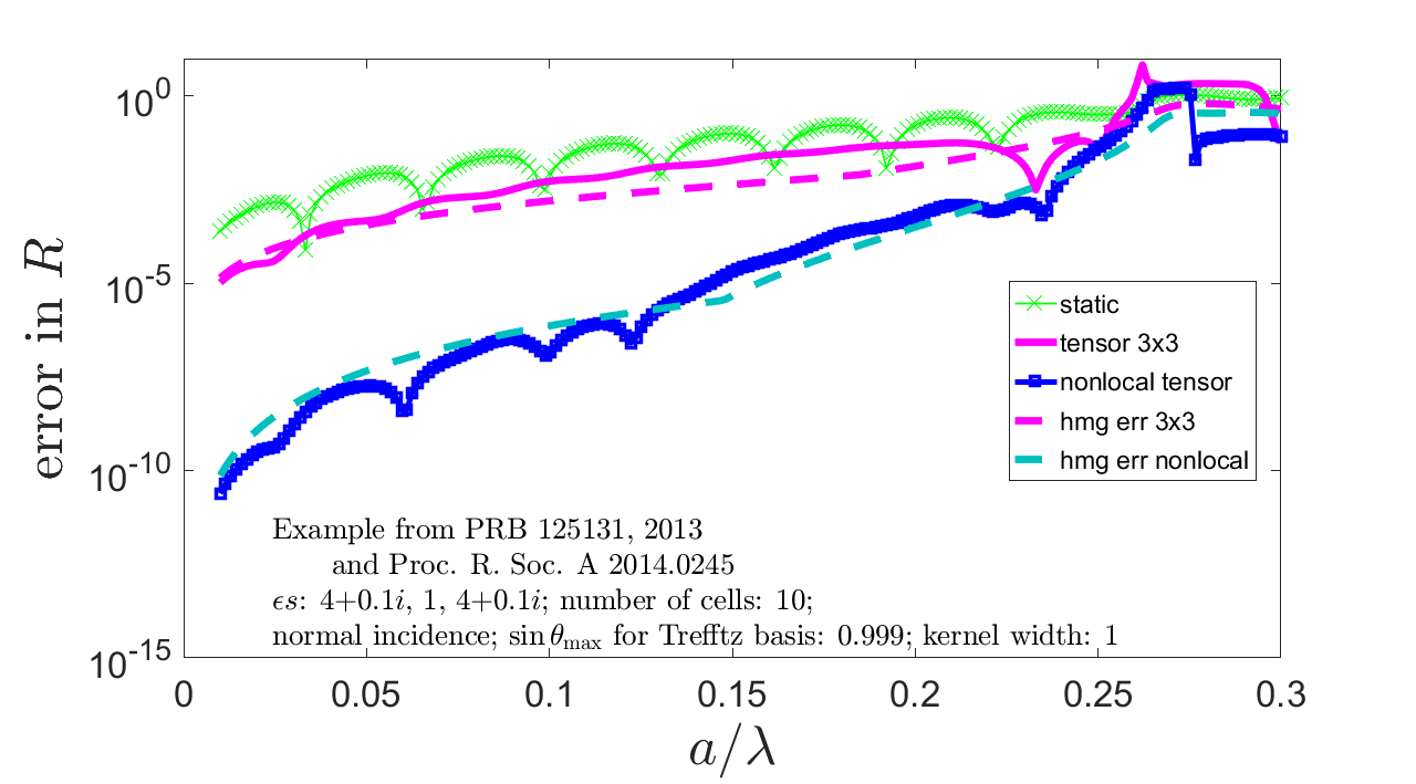
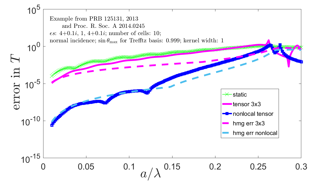
Shown in Figs. 2 and 3 are the reflection and transmission coefficients for electromagnetic waves propagating through a layered slab. These coefficients are defined in a standard way, as the ratio of the complex amplitudes of the reflected/transmitted waves to that of the incident wave. The geometric and physical parameters correspond to Example A of [41]: the lattice cell of a width contains three layers of widths , and , with scalar permittivities , , and , respectively; and . The fine-level Trefftz basis contains Bloch modes traveling at equispaced angles in ; . In nonlocal homogenization, the additional DoF are the integrals of the form (30), with the Gaussian kernel of width .
Fig. 2 shows the real part of and as a function of the angle of incidence, for . (The imaginary parts are not plotted to save space but are qualitatively similar). Since analytical solutions for wave propagation in layered media are fairly simple and well known, one may easily calculate the errors in and ; those are plotted in Fig. 3.
The figures show that our numerical results, especially for nonlocal homogenization, are highly accurate. In fact, we are not aware of any alternative methods that could produce a comparable level of accuracy at a comparable computational cost.22 2 The latter provision is needed to exclude from consideration “brute force” numerical optimization of the material tensor.
What explains this high accuracy? Plausible mechanisms are presented in Section 6.
5 Electromagnetic Waves in Slab Geometries
5.1 Formulation of the problem
The general description of the problem in this section closely follows the recently published paper [42], which explores a new computational method, “FLAME-slab,” for electromagnetic wave scattering problems in aperiodic photonic structures – specifically, structures possessing short-range regularity but lacking long-range order, such as amorphous or quasicrystalline lattices. Structures of this type can exhibit a variety of interesting properties, e.g. highly isotropic band gaps and fractal photonic spectra, but are difficult to study numerically [43, 44, 45, 46, 47, 48, 49, 50, 51, 52]. FLAME-slab exploits the short-range regularity of the structure by generating a Trefftz basis in a relatively small segment of the structure.
As an example, we consider a slab substrate patterned with aperiodically placed but geometrically identical pillars (Fig. 4). The slab has thickness , and there are 10 pillars of height and width . Both the substrate and the pillars have dielectric constant . The surrounding medium is air. In our calculations, we adopt computational units where the vacuum constants and the speed of light are all set to unity: , , . Then the frequency has the units of , where is the free space wavelength.
Light is incident from the top, as shown in Fig. 4, with a wavenumber and incidence angle relative to the -axis. We take the entire structure to be a supercell of length , with quasi-periodic boundary conditions (see below). The electric and magnetic fields in the structure are governed by Maxwell’s equations:
| (31) |
We consider the case where the electric field is -polarized, , so that the magnetic field has the form . The quasi-periodic boundary conditions are:
| (32) |
where is the -component of the incident wave vector .
The scattered electric field is defined as
| (33) |
where and are the total and incident electric fields, respectively. The magnetic field is split similarly. The scattered field is purely outgoing on both the upper side (towards the negative -direction) and the lower side (towards the positive -direction) of the structure.
Fig. 5(a) shows the discretization scheme for FLAME. The structure is discretized into grid points in the horizontal direction. In the vertical direction, the number of layers is deliberately limited to three (, , ), to demonstrate that FLAME-slab can work well on very coarse grids. The electric fields in these three layers are denoted with , , . Similarly, the magnetic fields in the upper and bottom layers are denoted with , .
We define three distinct types of patches, with their corresponding grid “molecules” and FD stencils. The first is a standard 9-point stencil containing just the electric field degrees of freedom (DoF), as shown in the left panel of Fig. 5(b). The second is a 6-point stencil over the middle and top layers, containing both the electric and magnetic fields (middle panel). The third is a 6-point stencil over the middle and bottom layers, containing both the electric and magnetic fields (right panel of Fig. 5(b)).
Each type of patch thus contains 9 degrees of freedom. FLAME uses 8 basis functions, to be determined by solving Maxwell’s equations for “Trefftz cells” matching the local dielectric environment in each patch. Each Trefftz cell contains a segment of length with a single pillar on the substrate; quasi-periodic boundary conditions are imposed. We choose , so that Maxwell’s equations can be solved much more rapidly for the Trefftz cell than for the entire aperiodic structure. We generate 8 different Trefftz basis functions by picking two different segment lengths ( and ), and four different angles of incidence for each . To compute the fields in the Trefftz cell, we use the existing rigorous coupled wave analysis (RCWA) solver [53].
The FLAME procedure now yields a matrix equation of the form
| (34) |
where is a matrix of stencil coefficients and is a column vector containing the nodal values of the total electric and magnetic fields. In our examples, has the size , and has the size ; we emphasize that this is just one possible choice of discretization, and other choices can be handled in a completely analogous way. Details about the calculation of can be found in [42].
FLAME schemes need to be supplemented with radiation boundary conditions. One way of implementing such conditions is via the Dirichlet-to-Neumann (DtN) maps in the semi-infinite air strips above and below the slab. DtN maps can be efficiently calculated via Fast Fourier Transforms (FFTs). More specifically, from Maxwell’s equations in free space,
| (35) |
The operating frequency , under the assumed normalization . We expand the scattered electric field into its Fourier series:
| (36) |
where the factor of comes from the quasiperiodic boundary conditions in the direction, with . The summation runs over the integer values, is the horizontal wavenumber, and
| (37) |
In the above equation, the choice of depends upon the layer we are dealing with ( for the upper layer and for the bottom layer), so that the scattered field is outgoing. Eqs. (35) and (36) give
| (38) |
The coefficients in (36) can be efficiently computed via a Fast Fourier Transform, and then the scattered magnetic field (38) can be obtained via the respective inverse transform (detailed expressions can be found in [54]). This leads to equations in the following matrix form:
| (39) |
where is a sparse sub-matrix obtained using FLAME, and is sub-matrix obtained from the boundary relations [42]. In our 2D examples, standard direct solvers in Matlab were sufficient for finding . In 3D, iterative solvers will need to be used, but this issue is completely beyond the scope of the present paper.
5.2 Results
Fig. 6 compares the fields calculated using FLAME-slab to a reference RCWA calculation. The structure is the one shown in Fig. 4, with frequency and incidence angle . For the FLAME-slab calculation, we take a horizontal discretization of , and precompute the Trefftz basis functions with (the number of expansion terms used in the RCWA subroutine [53]) and (the cell dicretization used for storing the Trefftz basis functions). The pure RCWA reference solution is computed using – an “overkill” setting meant to produce a highly accurate solution. The figure shows two representative field components: the real part of the scattered electric field () in the middle layer () in Fig. 6(a), and the scattered magnetic field () in the bottom layer () in Fig. 6(b). The FLAME-slab solution is seen to be in excellent agreement with the RCWA solution.
The central issue of this paper is approximation, and the finite-difference measure most closely related to it is the (normalized) consistency error
| (40) |
where Euclidean vector norms and the Frobenius matrix norm are implied.
In (40), should ideally be the exact solution, which is not available; hence an overkill RCWA solution with is used in its stead.
Since FLAME-slab contains a few adjustable parameters, we study the dependence of the consistency error on these parameters separately.
Fig. 7 displays the consistency error versus the incidence angle . For this calculation, we set , , and . The consistency error oscillates but remains bounded by over the entire range of .
Fig. 8 shows the consistency error versus the vacuum wavelength for the 10 pillar system, with fixed incidence angle . The FLAME-slab parameters are fixed at , , and . As is increased, decreases from to around . Past this point, saturates.
Fig. 9 shows the consistency error versus spatial discretization , for and normal incidence . The other FLAME-slab parameters are and . The consistency error decreases with , saturating at for .
For the purposes of the paper, the main qualitative conclusion of this section is that Trefftz functions, on which FLAME-slab is based, provide an accurate approximation of the electromagnetic field in a geometrically and physically complex structure.
6 The Accuracy of Trefftz Approximations
6.1 An Interpolation Argument
The numerical results for the two application examples of the previous sections show that Trefftz approximations are surprisingly effective. What explains their high accuracy?
As noted in Section 1, in the mathematical literature this question has been studied primarily for homogeneous subdomains (harmonic polynomials, plane/cylindrical/spherical wave expansions) but needs to be posed much more broadly, because complex inhomogeneous media are of great theoretical and practical interest. This section is an attempt to understand the general mechanisms of high accuracy of Trefftz approximations. Due to the complexity of this subject, some of the material, especially that of Section 6.3, is speculative and intended to stimulate further analysis and discussion.
In the case of Trefftz homogenization (Section 4), one can apply an interpolation argument using the summary in Section 2. Indeed, the key parameters in our homogenization methodology are the boundary averages of the Bloch fields (25). Each of these averages is, trivially, a periodic function of the angle (direction) of propagation of the respective Bloch wave and, as such, can be accurately approximated by the trigonometric interpolant over a set of equispaced knots. But these knots correspond precisely to the basis set of Bloch waves chosen in our procedure. Per Section 4, the accuracy of this interpolation is if the respective Bloch average is times continuously differentiable, or, under additional analyticity assumptions, even , where is the size of the Bloch basis set (which is the same as the number of interpolation knots).

In our second example of wave propagation and scattering in a slab geometry, the interpolation argument is not sufficient. This is because our Trefftz functions are defined over a segment of the structure, whereas the full electromagnetic problem is defined over the whole structure. Hence a more sophisticated explanation for the accuracy of Trefftz approximations in this case is needed.
We start with a slightly more abstract physical setup than that of Fig. 1. Namely, let us assume, as before, that an inhomogeneous scatterer occupies a Lipschitz domain (solid red in Fig. 10) which is enclosed in a shell (textured area). As previously, we consider a Trefftz “training set” corresponding to several incident waves, and are interested in approximating a different, generally unknown, solution in a small subdomain . This approximation can be used, for example, to generate a high-order difference scheme in , as was done in Section 5.
The Trefftz training set is also generated for fixed position-dependent parameters in . Importantly, however, the unknown solution may correspond to material parameters which differ in from those assumed for the training set (but are the same in ). The presence of the variable layer makes this case peculiar. The following section examines why accurate local Trefftz approximations can still be expected.
6.2 An Auxiliary “Reference” Basis
Let us assume that in there is an auxiliary basis () which can provide an accurate approximation of a (generic) solution of the wave equation:
| (41) |
Here is an error term, is a coefficient vector, and are some generic constants, the latter being “small” in some sense (see Theorems below). In the specific example of -wave scattering in Section 5, the unknown is the -field; but here we use the “generic” symbol as an indication that our analysis could be applied more broadly.
Assuming that (41) holds, one applies it to the training set of Trefftz waves, and arrives at the linear transformation
where column vectors are underlined; is the transformation matrix, and is the approximation error for the Trefftz functions in terms of the local basis. If , and if matrix is invertible, then
where the ‘+’ subscript indicates the Moore-Penrose pseudoinverse.

The solution in can therefore be expressed as
| (42) |
where is the approximation error of this solution via the basis. Thus the smallness of the Trefftz approximation error hinges on the smallness of the norm of the pseudoinverse – that is, on the inverse of its minimum singular value ; we discuss that below.
The transformations above are schematically illustrated in Fig. 11. If the Trefftz basis and the solution can be approximated via the reference basis as in (41), and if is bounded from below, then one can approximate via the Trefftz basis (by following, conceptually, the two solid arrows in the sketch).
An example of this auxiliary basis is, in the special case of a homogeneous domain , a set of cylindrical harmonics , ; is the Bessel function of the first kind. Detailed error analyses have been carried out by Melenk, Hiptmair, Moiola and Perugia [25, 22, 55]. For our purposes, the most convenient final results can be found in [4, 26].
[4, Theorem 4]. Let be a simply connected, bounded Lipschitz domain. Let and assume that solves the homogeneous Helmholtz equation on . ¹ Then
| (43) |
where , ; depend only on , , and the wavenumber .
Under the assumptions of this theorem, the presence of a “buffer region” ensures that high-order harmonics from the boundary of die out sufficiently. If this assumption is not made, an alternative error estimate, dependent on the level of smoothness of the solution, reads:
[4, Theorem 5]. Let be a simply connected, bounded Lipschitz domain, star-shaped with respect to a ball. Let the exterior angle of be bounded from below by , . Assume that , , satisfies the homogeneous Helmholtz equation. Then33 3 There is an apparent misprint in [4]: instead of in the norm on the right hand side.
| (44) |
Obviously, in our case plays the role of the generic in the estimates above. These estimates of the error term in (41) are valid for the 2D Helmholtz equation in a physically homogeneous medium within .
Also in the special case of a homogeneous domain , and the Trefftz set consisting of plane waves traveling in equispaced angular directions, the norm of the pseudoinverse can be evaluated explicitly. From the Jacobi-Anger expansion, the entries of the matrix are
| (45) |
This matrix corresponds to a discrete Fourier transform, and its columns are easily shown to be orthogonal, so that
| (46) |
where is the identity matrix of dimension . It then immediately follows that
| (47) |
so in this case stability of the transformation is guaranteed.
6.3 A Connection with Random Matrix Theory
A natural, and critical, question is whether the well-posedness of the transformation noted above is accidental and valid in special cases only, or whether it has broader applicability. Practical experience with multiparticle problems, random and quasi-random structures of different kind [17, 18, 19, 23, 42], [35, Chapters 4, 6] strongly suggests the latter. Rigorous mathematical analysis is so far available only for a narrow subset of cases [25, Chapter IV], [26, Section 3], [27, 28], and may constitute an interesting direction of future research.
In the remainder of this section, we outline – on physical grounds – a curious connection between the accuracy of Trefftz approximations and the theory of random matrices. This theory dates back to von Neumann and Wigner [56, 57] and is now quite mature [58, 59, 60, 61, 62]. Particularly relevant to us is the following result.
Rudelson & Vershynin [62, Theorem 3.3].
Let be an random matrix whose entries are independent
and identically distributed (i.i.d.) subgaussian random variables
with zero mean and unit variance. Then
where and depend only on the subgaussian moment of the entries.
The connection of this theorem with the previous subsection can be outlined as follows.
- 1.
The Trefftz “training set” can be viewed as a particular realization of some random distribution (e.g. angles of incidence randomly chosen and/or random properties of the “shell” ). A notable feature of random matrix theory is universality: only mild dependence of the spectral bounds on the distribution of the random variables.
- 2.
One major restrictive condition, however, is that the matrix entries be i.i.d. variables. Strictly speaking, this condition can be immediately ascertained only under additional symmetry assumptions, e.g. the bases being invariant under rotation by a given angle. It is hoped that such strong assumptions can be relaxed.
- 3.
The assumption of zero mean is less restrictive and valid if the probability distribution of each function in the Trefftz training set , for all , is invariant with respect to the sign change of that function.
- 4.
Clearly, the theorem is applied with , .
- 5.
The assumption that the distribution is subgaussian is satisfied, in particular, by all bounded random variables and hence is not restrictive.44 4 A random variable is called subgaussian if there exists a positive constant such that for .55 5 There is an apparent misprint in [62]: instead of .
- 6.
Complex bases and matrices can be decomplexified by the substitutions of the form , . This preserves the relevant norms and hence does not affect the spectral bounds.
- 7.
The assumption of unit variance is obviously a matter of scaling only.
The theorem affirms that stability (47) of the transformation is not accidental. In fact, with a probability close to one, is not small, for any reasonable choice of the Trefftz basis.
7 Conclusion
The key argument of this paper is that Trefftz approximations – that is, approximations by functions satisfying (locally) a given differential equation – deserve to be studied and applied more broadly than is traditionally done. Conventionally, these approximations are used in homogeneous subdomains, where the underlying differential equation has constant coefficients; this is done in various contexts (GFEM, DG, FD).
As an illustration of a much broader use of Trefftz functions, the paper reviews two disparate but representative examples: (i) non-asymptotic and nonlocal two-scale homogenization of periodic electromagnetic media, and (ii) special Trefftz FD (FLAME) schemes for wave scattering from photonic structures with slab geometries. In both cases, Trefftz approximations are applied in complex inhomogeneous domains and prove to be quite effective.
We discuss possible mechanisms engendering the high accuracy of Trefftz approximations. One such mechanism is trigonometric interpolation, which itself is known to be surprisingly accurate for smooth periodic functions, in comparison with other typical forms of interpolation. We also outline, on physical grounds, a curious connection of Trefftz approximations with the theory of random matrices.
It is hoped that these considerations will stimulate further mathematical research and practical applications of Trefftz-based methods.
Acknowledgment
The work of IT was supported in part by the US National Science Foundation Grants DMS-1216927 and DMS-1620112. The research of SM and YC was supported by the Singapore MOE Academic Research Fund Tier 2 Grant MOE2016-T2-1-128, the Singapore MOE Academic Research Fund Tier 2 Grant MOE2015-T2-2-008, and the Singapore MOE Academic Research Fund Tier 3 Grant MOE2016-T3-1-006. The work of VM was supported in part by the US National Science Foundation Grants DMS-1216970.
IT thanks Ralf Hiptmair, Andrea Moiola, Lise-Marie Imbert-Gérard and Ben Schweizer for discussions.
References
References
- [1] I. Herrera, Trefftz method: A general theory, Numer. Methods Partial Differential Eq. 16 (2000) 561–580.
- [2] C. Farhat, R. Tezaur, J. Toivanen, A domain decomposition method for discontinuous Galerkin discretizations of Helmholtz problems with plane waves and Lagrange multipliers, International Journal for Numerical Methods in Engineering 78 (13) (2009) 1513–1531. doi:10.1002/nme.2534.
- [3] J. Melenk, I. Babuška, The partition of unity finite element method: Basic theory and applications, Comput. Methods Appl. Mech. Engrg. 139 (1996) 289–314.
- [4] I. Babuška, J. Melenk, The partition of unity method, Int. J. for Numer. Meth. in Eng. 40 (4) (1997) 727–758.
- [5] I. Babuška, U. Banerjee, J. E. Osborn, Generalized finite element methods – main ideas, results and perspective, International Journal of Computational Methods 1 (1) (2004) 67–103. doi:10.1142/S0219876204000083.
- [6] A. Plaks, I. Tsukerman, G. Friedman, B. Yellen, Generalized Finite Element Method for magnetized nanoparticles, IEEE Trans. Magn. 39 (3) (2003) 1436–1439.
- [7] L. Proekt, I. Tsukerman, Method of overlapping patches for electromagnetic computation, IEEE Trans. Magn. 38 (2) (2002) 741–744.
- [8] T. Strouboulis, I. Babuška, R. Hidajat, The generalized finite element method for Helmholtz equation: Theory, computation, and open problems, Computer Methods in Applied Mechanics and Engineering 195 (37) (2006) 4711 – 4731, John H. Argyris Memorial Issue. Part I. doi:10.1016/j.cma.2005.09.019.
- [9] B. Cockburn, G. Karniadakis, C.-W. Shu, The development of discontinuous Galerkin methods, in: B. Cockburn, G.E.Karniadakis, C.-W.Shu (Eds.), Discontinuous Galerkin Methods. Theory, Computation and Applications, Vol. 11 of Lecture Notes in Comput. Sci. Engrg., Springer-Verlag, New York, 2000, pp. 3–50.
- [10] D. N. Arnold, F. Brezzi, B. Cockburn, L. D. Marini, Unified analysis of discontinuous Galerkin methods for elliptic problems, SIAM J. Numer. Analysis 39 (5) (2002) 1749–1779.
- [11] A. Buffa, P. Monk, Error estimates for the ultra weak variational formulation of the Helmholtz equation, M2AN, Math. Model. Numer. Anal. 42 (6) (2008) 925–940.
- [12] C. J. Gittelson, R. Hiptmair, I. Perugia, Plane wave discontinuous Galerkin methods: Analysis of the h-version, ESAIM: M2AN 43 (2) (2009) 297–331. doi:10.1051/m2an/2009002.
- [13] G. Gabard, P. Gamallo, T. Huttunen, A comparison of wave-based discontinuous Galerkin, ultra-weak and least-square methods for wave problems, International Journal for Numerical Methods in Engineering 85 (3) (2011) 380–402. doi:10.1002/nme.2979.
- [14] R. Hiptmair, A. Moiola, I. Perugia, Plane wave discontinuous Galerkin methods for the 2d Helmholtz equation: Analysis of the p-version, SIAM Journal on Numerical Analysis 49 (1) (2011) 264–284. doi:10.1137/090761057.
- [15] F. Kretzschmar, A. Moiola, I. Perugia, S. M. Schnepp, A priori error analysis of space–time Trefftz discontinuous Galerkin methods for wave problems, IMA Journal of Numerical Analysis 36 (4) (2016) 1599–1635.
- [16] I. Tsukerman, Trefftz difference schemes on irregular stencils, J of Comput Phys 229 (8) (2010) 2948–2963.
- [17] I. Tsukerman, Electromagnetic applications of a new finite-difference calculus, IEEE Trans. Magn. 41 (7) (2005) 2206–2225.
- [18] I. Tsukerman, A class of difference schemes with flexible local approximation, J. Comput. Phys. 211 (2) (2006) 659–699.
- [19] I. Tsukerman, F. Čajko, Photonic band structure computation using FLAME, IEEE Trans Magn 44 (6) (2008) 1382–1385.
- [20] E. Deckers, O. Atak, L. Coox, R. D’Amico, H. Devriendt, S. Jonckheere, K. Koo, B. Pluymers, D. Vandepitte, W. Desmet, The wave based method: An overview of 15 years of research, Wave Motion 51 (4) (2014) 550 – 565, Innovations in Wave Modelling. doi:10.1016/j.wavemoti.2013.12.003.
- [21] Q. Qin, Trefftz finite element method and its applications, ASME Appl. Mech. Rev. 58 (5) (2005) 316–337. doi:doi:10.1115/1.1995716.
- [22] R. Hiptmair, A. Moiola, I. Perugia, A Survey of Trefftz Methods for the Helmholtz Equation, Springer International Publishing, 2016, pp. 237–279. doi:10.1007/978-3-319-41640-3_8.
- [23] J. Dai, H. Pinheiro, J. Webb, I. Tsukerman, Flexible approximation schemes with numerical and semi-analytical bases, COMPEL 30 (2) (2011) 552–573.
- [24] E. Perrey-Debain, Plane wave decomposition in the unit disc: Convergence estimates and computational aspects, Journal of Computational and Applied Mathematics 193 (1) (2006) 140 – 156. doi:10.1016/j.cam.2005.05.027.
- [25] J. M. Melenk, On generalized finite element methods, PhD Thesis, Univ. of Maryland (1995).
- [26] J. Melenk, Operator adapted spectral element methods I: harmonic and generalized harmonic polynomials, Numer. Math. 84 (1999) 35–69.
- [27] O. Laghrouche, P. Bettess, E. Perrey-Debain, J. Trevelyan, Wave interpolation finite elements for helmholtz problems with jumps in the wave speed, Computer Methods in Applied Mechanics and Engineering 194 (2) (2005) 367 – 381, Selected papers from the 11th Conference on The Mathematics of Finite Elements and Applications. doi:10.1016/j.cma.2003.12.074.
- [28] L.-M. Imbert-Gérard, Interpolation properties of generalized plane waves, Numer. Math. 131 (4) (2015) 683–711. doi:10.1007/s00211-015-0704-y.
- [29] G. Meinardus, Approximation of Functions: Theory and Numerical Methods, Springer, 1967.
- [30] D. Jackson, The Theory of Approximation, no. v. 11 in Colloquium Publications – American Mathematical Society, Amer Mathematical Society, 1930.
- [31] E. W. Cheney, T. J. Rivlin, Some polynomial approximation operators, Mathematische Zeitschrift 145 (1) (1975) 33–42. doi:10.1007/BF01214496.
- [32] A. P. Austin, L. N. Trefethen, Trigonometric interpolation and quadrature in perturbed points, SIAM Journal on Numerical Analysis 55 (5) (2017) 2113–2122. doi:10.1137/16M1107760.
- [33] A. P. Austin, Some new results on and applications of interpolation in numerical computation, D. Phil. Thesis (2016).
- [34] L. N. Trefethen, J. A. C. Weideman, The exponentially convergent trapezoidal rule, SIAM Review 56 (3) (2014) 385–458. doi:10.1137/130932132.
- [35] I. Tsukerman, Computational Methods for Nanoscale Applications: Particles, Plasmons and Waves, Springer, 2007.
- [36] H. Pinheiro, J. Webb, I. Tsukerman, Flexible local approximation models for wave scattering in photonic crystal devices, IEEE Trans. Magn. 43 (4) (2007) 1321–1324. doi:0.1109/TMAG.2006.891004.
- [37] A. Boag, A. Boag, R. Mittra, Y. Leviatan, A numerical absorbing boundary-condition for finite-difference and finite-element analysis of open structures, Microwave & Opt Tech Lett 7 (9) (1994) 395–398.
- [38] I. Babuška, F. Ihlenburg, E. T. Paik, S. A. Sauter, A generalized finite element method for solving the Helmholtz equation in two dimensions with minimal pollution, Comput Meth Appl Mech & Eng 128 (1995) 325–359.
- [39] I. Tsukerman, Classical and non-classical effective medium theories: New perspectives, Physics Letters A 381 (19) (2017) 1635 – 1640. doi:http://doi.org/10.1016/j.physleta.2017.02.028.
- [40] I. Tsukerman, V. A. Markel, A nonasymptotic homogenization theory for periodic electromagnetic structures, Proc Royal Society A 470 (2014) 2014.0245. doi:10.1098/rspa.2014.0245.
- [41]
V. A. Markel, I. Tsukerman,
Current-driven
homogenization and effective medium parameters for finite samples, Phys.
Rev. B 88 (2013) 125131.
doi:10.1103/PhysRevB.88.125131.
URL http://link.aps.org/doi/10.1103/PhysRevB.88.125131 - [42] S. Mansha, I. Tsukerman, Y. Chong, The FLAME-slab method for electromagnetic wave scattering in aperiodic slabs, Optics Express 25 (2017) 32602–32617.
- [43]
C. Jin, X. Meng, B. Cheng, Z. Li, D. Zhang,
Photonic gap in
amorphous photonic materials, Phys. Rev. B 63 (2001) 195107.
doi:10.1103/PhysRevB.63.195107.
URL https://link.aps.org/doi/10.1103/PhysRevB.63.195107 - [44]
P. García, R. Sapienza, A. Blanco, C. López,
Photonic glass: A novel
random material for light, Advanced Materials 19 (18) (2007) 2597–2602.
doi:10.1002/adma.200602426.
URL http://dx.doi.org/10.1002/adma.200602426 - [45]
M. Florescu, S. Torquato, P. J. Steinhardt,
Designer disordered
materials with large, complete photonic band gaps, Proceedings of the
National Academy of Sciences 106 (49) (2009) 20658–20663.
doi:10.1073/pnas.0907744106.
URL http://www.pnas.org/content/106/49/20658.abstract - [46]
H. Noh, J.-K. Yang, S. F. Liew, M. J. Rooks, G. S. Solomon, H. Cao,
Control of
lasing in biomimetic structures with short-range order, Phys. Rev. Lett. 106
(2011) 183901.
doi:10.1103/PhysRevLett.106.183901.
URL https://link.aps.org/doi/10.1103/PhysRevLett.106.183901 - [47]
H. K. Liang, B. Meng, G. Liang, J. Tao, Y. Chong, Q. J. Wang, Y. Zhang,
Electrically pumped
mid-infrared random lasers, Advanced Materials 25 (47) (2013) 6859–6863.
doi:10.1002/adma.201303122.
URL http://dx.doi.org/10.1002/adma.201303122 - [48]
S. Mansha, Z. Yongquan, Q. J. Wang, Y. D. Chong,
Optimization
of tm modes for amorphous slab lasers, Opt. Express 24 (5) (2016)
4890–4898.
doi:10.1364/OE.24.004890.
URL http://www.opticsexpress.org/abstract.cfm?URI=oe-24-5-4890 - [49]
Z. Feng, X. Zhang, Y. Wang, Z.-Y. Li, B. Cheng, D.-Z. Zhang,
Negative
refraction and imaging using 12-fold-symmetry quasicrystals, Phys. Rev.
Lett. 94 (2005) 247402.
doi:10.1103/PhysRevLett.94.247402.
URL https://link.aps.org/doi/10.1103/PhysRevLett.94.247402 - [50]
W. Steurer, D. Sutter-Widmer,
Photonic and phononic
quasicrystals, Journal of Physics D: Applied Physics 40 (13) (2007) R229.
URL http://stacks.iop.org/0022-3727/40/i=13/a=R01 - [51]
S. F. Liew, S. Knitter, W. Xiong, H. Cao,
Photonic crystals
with topological defects, Phys. Rev. A 91 (2015) 023811.
doi:10.1103/PhysRevA.91.023811.
URL https://link.aps.org/doi/10.1103/PhysRevA.91.023811 - [52]
S. Knitter, S. F. Liew, W. Xiong, M. I. Guy, G. S. Solomon, H. Cao,
Topological defect
lasers, Journal of Optics 18 (1) (2016) 014005.
URL http://stacks.iop.org/2040-8986/18/i=1/a=014005 - [53]
V. Liu, S. Fan,
S4
: A free electromagnetic solver for layered periodic structures, Computer
Physics Communications 183 (10) (2012) 2233 – 2244.
doi:http://dx.doi.org/10.1016/j.cpc.2012.04.026.
URL http://www.sciencedirect.com/science/article/pii/S0010465512001658 - [54] S. Mansha, Amorphous photonic structures, PhD Thesis, Nanyang Technological University, Singapore (2018).
- [55] A. Moiola, Trefftz-Discontinuous Galerkin Methods for Time-Harmonic Wave Problems, Ph.D. thesis, ETH Zurich (2011).
- [56] J. von Neumann, H. Goldstine, Numerical inverting of matrices of high order, Bull. Amer. Math. Soc. 53 (11) (1947) 1021–1099.
- [57]
E. P. Wigner, Characteristic vectors
of bordered matrices with infinite dimensions, Annals of Mathematics 62 (3)
(1955) 548–564.
doi:10.2307/1970079.
URL http://www.jstor.org/stable/1970079 - [58] G. Akemann, J. Baik, P. D. Francesco, The Oxford Handbook of Random Matrix Theory, Oxford: Oxford University Press, 2011.
- [59]
T. Tao, V. Vu, Random
matrices: the distribution of the smallest singular values, Geometric and
Functional Analysis 20 (1) (2010) 260–297.
doi:10.1007/s00039-010-0057-8.
URL https://doi.org/10.1007/s00039-010-0057-8 - [60] M. Rudelson, R. Vershynin, The least singular value of a random rectangular matrix, Comptes rendus de l’Acadmie des sciences – Mathmatique 346 (2008) 893–896.
- [61]
M. Rudelson, R. Vershynin, Smallest
singular value of a random rectangular matrix, Communications on Pure and
Applied Mathematics 62 (12) (2009) 1707–1739.
doi:10.1002/cpa.20294.
URL http://dx.doi.org/10.1002/cpa.20294 - [62] M. Rudelson, R. Vershynin, Non-asymptotic theory of random matrices: extreme singular values, in: Proceedings of the International Congress of Mathematicians, Hyderabad, India, 2010.