Stability, convergence, and sensitivity analysis of the FBLM and the corresponding FEM
Abstract
This paper focuses on the study of the filament based lamellipodium model (FBLM) and the corresponding finite element method (FEM) from a numerical point of view. We study fundamental numerical properties of the FEM and justify the further use of the FBLM. We exhibit that the FEM satisfies a timestep stability condition that is consistent with the nature of the problem. We propose a particular strategy to automatically adapt the time step of the method. We show that the FEM convergences with respect to the (two-dimensional) space discretization in a series of characteristic and representative experiments. We embed and couple the FBLM with a complex extracellular environment comprised of chemical and haptic components and study their combined time evolution. Under this prism, we study the sensitivity of the FBLM on several of its controlling parameters and discuss their influence in the development of the model.
1 Introduction
Fibroblasts, keratocytes, cancer cells, and other types of fast moving cells exhibit a particular crawling-like motion in which the lamellipodium of the cells plays a pivotal role, Small et al. (2002); Svitkina et al. (1997); Yam et al. (2007); Postlethwaite and Keski-Oja (1987); Gerisch and Keller (1981); Iijima et al. (2002); Zigmond and Hirsch (1973).
The lamellipodium is a sheet-like dense network that can be found in the propagating front of the cells and is comprised of linear biopolymers of the protein actin —termed actin-filaments or simply filaments.. These actin-filaments are highly dynamic; they continuously polymerize, adhere to the substrate, and are subject to numerous other processes like nucleation, fragmentation, capping, and more Blanchoin et al. (); Lauffenburger and Horwitz (1996); Gittes et al. (1993); Tojkander et al. (2012); Mitchison and Cramer (1996); Jay et al. (1995); Chen (1981).
These processes affect the structure and the functionality of the lamellipodium and the motility of the cell, Small et al. (2002). They are influenced, to a large extent, by the extracellular environment, its chemical composition and the architecture of the Extracellular Matrix (ECM). The response of the cell to gradients of extracellular chemical signals and ECM-bound adhesion sites is termed chemotaxis and haptotaxis respectively.
There have been several approaches in the literature to model and simulate lamellipodium driven cell motility. In the current paper we do not aim to develop a new model or to perform biologically relevant numerical experiments, hence we do not discuss the literature in detail or compare the different models. We merely refer the interested reader to some of the existing works Sabass and Schwarz (2010); Fuhrmann and Stevens (2015); Marth et al. (2015); Rubinstein et al. (2009); Alt and Kuusela (2009); Cardamone et al. (2011); Scianna et al. (2013); Möhl et al. (2012); Madzvamuse and George (2013); Ambrosi and Zanzottera (2016).
The model we follow is the Filament Based Lamellipodium Model (FBLM), a two dimensional, two phase model that describes the lamellipodium at the level of actin-filaments. It was first introduced in Oelz et al. (2008); Oelz and Schmeiser (2010a) and was further extended in Manhart et al. (2015). When endowed with a particular problem specific Finite Element Method (FEM), the the resulting FBLM-FEM is able to reproduce a realistic, crawling-like lamellipodium driven motility Manhart et al. (2016); Brunk et al. (2016).
Although the FBLM describes the dynamics of the actin-filaments and the lamellipodium, the deduced motility is understood as the motility of the full cell. This is due to the fact that the role of the lamellipodium in the motility of the model biological cell (fish keratocyte) is predominant, Small et al. (2002). We henceforth will not distinguish between the two, and for convenience we will use the term cell motility for both cases.
The FBLM and the corresponding FEM have been used so far in several works to simulate various cases of cell motility, e.g. Manhart et al. (2015); Manhart et al. (2016); Brunk et al. (2016). To date though no numerical investigations have been presented in the literature to verify that the FBLM-FEM combination satisfies some (at least minimum) numerical prerequisites and justify thusly its further use in biological relevant situations. What moreover is missing from the relevant literature is a study of the corresponding parameters and of the effect they have on the dynamics of the FBLM. Such parameter study would facilitate the parameter identification procedure in the reproduction/simulation of realistic biological experiments. The current work aims to partially fill these gaps and is split in two main parts.
In the first part of the paper, we identify appropriate timestep stability conditions in chemotaxis and haptotaxis experiments where we propose a relation between the time and the (two-dimensional) “space” discretization steps. We investigate the dependence of the stability constant on the gradient of the ECM and propose an adaptive time control (ATC) method for the automatic adaptation of the timestep of the numerical method.
We also exhibit the convergence of the FEM. For that we consider three generic and representative experiments and a discretization grid that is refined with respect to both “spatial” variables.
As the model and the numerical method are quite complex, they do not allow for a rigorous numerical analysis study; as a result we restrict our work here to the experimental and case dependent study of these properties and postpone the more rigorous numerical and analytical investigations for a separate work. Nevertheless, the benefit that stems from the first part of our work is mainly the verification that the FBLM-FEM can be further employed in biologically relevant numerical simulations. Most notably, that the refinement of the mesh and the adaptation of the timestep will be able to reveal the dynamics of the model.
In the second part of the paper, we make one more step towards biological realism and embed the FBLM in a complex and adaptive chemical and haptic extracellular environment. Such extended FBLM-environment model combination will allow us to better reproduce in vitro biological experiments. The model for the environment we propose here is minimal. It includes only some basic components of the extracellular environment and we use it primarily to present the FBLM-environment coupling.
Based on the FBLM-environment combination, we perform a sensitivity analysis in a generic experimental case, where we identify the most influential parameters and address the effect they have in the dynamics of the model. We get this way a critical insight of the different components and dynamics of the FBLM and pave the way for more detailed and problem specific parameter identification investigations and the simulation of biologically relevant experimental scenarios.
The structure of the paper is as follows: in Section 2 we describe briefly the FBLM and give some details on extensions of the model that we consider for the first time. In Sections 3 and 4 we study the stability and the convergence of the the FEM. In Section 5 we introduce the model for the extracellular environment, and in Section 6, we study the sensitivity of the FBLM-FEM on a series of its controlling parameters. In the Appendix we provide some basic information on the FEM and the FV methods we use to solve the FBLM and the environment.
2 The FBLM
We present here some information on the FBLM and the new components that we include, and refer to Oelz et al. (2008); Oelz and Schmeiser (2010a); Oelz and Schmeiser (2010b); Manhart et al. (2015); Manhart et al. (2016); Brunk et al. (2016) for more details.
The FBLM is a two-dimensional, two-phase continuum model that describes the dynamics of the lamellipodium by retaining key biological processes of the actin-filaments, the interactionswith each other, as well as their interactions with the extracellular environment.
The main assumptions behind the FBLM are a) the lamellipodium is a two dimensional structure, and b) the actin filaments are organized in two locally parallel families (denoted here by the superscripts or ). Each family covers a region with the filaments connecting the membrane with the inside of the cell.
The filaments of the family are indexed by and have a maximal length at time . The two families are parametrized with respect to their arclength as
| (1) |
and coincide at their outer boundaries () with the membrane of the cell
| (2) |
They moreover satisfy the constraint
| (3) |
that is understood as an inextensibility condition between their monomers.
We assume that filaments of the same family do not intersect each other
| (4) |
and that filaments of different families cross at most once
| (5) |
In the heart of the FBLM is found the system of equations
| (6) |
where and where we have dropped the notation and focus on one of the two families/equations. The other family is indicated by the superscript ∗ for which a similar equation holds.
The function represents the (number) density of filaments of length at least at time with respect to . The corresponding submodels used to derive the evolution of (and ) incorporate the effects of polymerization, depolymerization, branching, and capping, see Manhart et al. (2015).
The first term on the right hand side of (6) describes the resistance of the filaments against bending, the second term is a tangential tension force, stemming from the inextensibility constraint (3) with the Lagrange multiplier . The third term describes the friction between the filament network and the substrate.
The filaments polymerize at the leading edge with rate . The material derivative operator
describes the velocity of the actin-material relative to the substrate. In a similar way we set .
The pressure effect in (6) is caused by Coulomb repulsion between neighbouring filaments of the same family with pressure given by the density of actin as
| (7) |
The last two terms in (6) model the interaction between the two families caused by elastic cross-links and/or branch junctions. The first one describes the resistance against changing the angle
between crossing filaments away from the equilibrium angle of the cross-linking molecule. The second one describes the friction between the two families analogously to the friction with the substrate.
The system (6) is subject to the boundary conditions
| (8) | ||||
The terms in the second line, describe forces applied to the filament ends. The force in the direction orthogonal to the leading edge at arises from the constraint (2) with the Lagrange parameter . The forces at the inner boundary model the contraction effect of actin-myosin interaction in the interior region, refer to Manhart et al. (2015) for details.
Fundamental to the motility of the cell, is the breaking of the symmetry in the thickness of the lamellipodium. This way, the effective pulling force becomes stronger in the direction of the wider lamellipodium Yam et al. (2007). The maximal length of the filaments and width of the lamellipodium , depends on the polymerization rate. Based on the capping, severing, and filament nucleation procedures, we have deduced in Manhart et al. (2015) the relation
| (11) |
which reveals the direct dependence of the width of the lamellipodium to the polymerization rate of of the local filaments.
For more details on the FBLM we refer to Oelz et al. (2008); Oelz and Schmeiser (2010a); Oelz and Schmeiser (2010b); Manhart et al. (2015); Manhart et al. (2016).
Adjusting the polymerization rate
We consider in this work two mechanisms to control the polymerization rate of the filaments. The first is the direct response of the intracellular polymerization mechanism to extracellular chemical signals as they are perceived by the cell through transmembrane receptors. The second mechanism represents (unspecified in this paper) intracellular processes that destabilize, cut off, or even enhance the response of the polymerization mechanism.
For the first mechanism we assume that the polymerization rate of the filament is adjusted between the minimum and the maximum value , of the cell polymerization mechanism according to the density of the extracellular chemical signal (that serves as a chemo-attractant) by the formula
| (12) |
where is the density of the extracellular chemical at the barbed end of the filament at time , i.e
The coefficient represents the response of the cell and in particular of the polymerization mechanism to changes of the extracellular chemical. Larger values lead to more pronounced changes of the polymerization rate and to more polarized cells.
The exponential function in (12) has no biological justification; it is used merely to provide a smooth transition from the minimum to the maximum polymerization rate in a continuous and controlled manner. Other functions with the same attributes could be used in its place.
The second mechanism that we consider describes primarily intracellular processes. For biological reasons that are not specified in this work, the polymerization mechanism can be hampered or otherwise destabilized, leading to an assortment of phenomena like persistent very high or low polymerization rates, abrupt changes of the polymerization rate, etc. This part of the model was previously proposed in Manhart et al. (2015) where it was used to prescribe the polymerization rate directly on the membrane of the cell.
The conditions that destabilize the polymerization mechanism are important in a assortment of phenomena (pathological or not) which are beyond the scope of this paper, so we will not comment on them any more. We understand though the biological significance of both mechanisms as well as their distinctive functionality and use both of them in this work.
Overall, the polymerization rate that we consider is given as
| (13) |
where describes the internal controlling mechanism that can potentially depend on a large number of cellular processes. Nevertheless, unless otherwise stated, we assume throughout this paper that and hence
| (14) |
For the numerical solution of the FBLM we employ a problem specific FEM that we briefly describe in Appendix A. It was previously developed in Manhart et al. (2016); Brunk et al. (2016), where we refer for more details.
 |
 |
| (a) | (b) |
3 Timestep stability
The complexity of the FBLM (6) and the FEM (35) do not allow for a rigorous stability analysis. Instead, we perform here an experimental/numerical investigation where we exhibit the existence of regions of stability for the timestep in terms of the space discretizaiton steps and .
To this end, we first note that the structure of the FEM (37)–(41) indicates a particular relation between , , and , of the form:
| (15) |
To identify the stability constant , we numerically solve indicative experiments for different combinations of , , . For each combination, we characterize the resulting conformation as smooth (or not) and accordingly accept (or not) the corresponding combination. The largest to result to smooth solutions gives rise to . As we see later, this procedure can be used to set the timestep of the method in an automated way.
The experiments that we consider are particular; one chemotaxis and one haptotaxis. In the fist we exhibit the approach we follow to identify the stability constraint, and discuss a computational approach to set the timestep automatically. In the second we go one step further and identify the relation between the stability constraint as the gradient of the ECM.
The first experiment we consider is a chemotaxis driven cell migration.
Experiment 3.1 (Stability – Chemotaxis)
An initially rotational symmetric cell migrates under the influence of a chemical signal. The direction and strength of the signal and the final simulation time are chosen in a way that the deformation and migration of the cell is small, while at the same time the width of the lamellipodium (and hence the effective pulling force) becomes significantly asymmetric around the lamellipodium.
The parameters for this experiment are given in Table 3. The polymerization rate varies smoothly from the minimum value at the posterior side of the cell, to the maximum value at the anterior, see Manhart et al. (2015) for more details.
 |
 |
| (a) | (b) |
As a first step for the computation of , we set the resolution of in (36) to be and , along the and directions respectively. Accordingly, (15) recasts to . Using Experiment 3.1 and varying by small increments we identify two smooth conformations: one for and one for , cf. Figure 2. When these timesteps are combined with (15) they yield respectively
| (16) |
To distinguish between these two values of , we consider the coarser grid with and and we deduce from (15) and (16) the timesteps and respectively. We test these values in Experiment 3.1 and note that in both cases the conformation of the lamellipodium is “smooth”, cf. Figure 3. In the case though, the corresponding polymerization rate functions are non smooth; this implies timestep driven numerical instabilities in the solution. In effect, the value is too large, and hence we promote the value .
We verify this stability constant with an even coarser grid with and . This time, we deduce from (16) and (15), the timesteps and respectively. The simulation results are shown in Figure 4, where we note that when the filaments in the lamellipodium and the polymerization rates are not smooth. Hence, we promote once again the stability constant
| (17) |
 |
 |
| (a) | (b) |
It is understood that this stability constant depends on a number of environmental parameters and variables, most notably on the extracellular chemical and matrix. Nevertheless, it is important to note that the FEM clearly exhibits stability regions with respect to the time and space steps and , .
Choosing the timestep
What we have seen by the previous analysis is that the stability of the method can be identified by the smoothness of the polymerization rate and the filament density functions. Using this information we can adjust the timestep of the method in an automated way, similar to the adaptive timestep control (ATC) methods, Hundsdorfer and Verwer (2003). For that, we propose to use the divided difference smoothness measure LeVeque (); Kolbe et al. (2016) or the smoothness indicators used in weighted essentially non-oscillatory (WENO) schemes, see e.g. Shu (2009).
In some more detail, we consider the discrete polymerization rate (and/or the filament density) function of the filaments at the end of one timestep of the method, see e.g. upper right panel in Figures 2, 3, 4.
The smoothness indicator is computed for as
| (18) |
where the “boundary” terms and are computed periodically with respect to , and where (by construction). The formula (18) is derived from a fourth order polynomial fitted to the numerical values . This “assumption” is made to meet the smoothness of the FEM shape functions, i.e. third order along the - and first order along the -direction, see (38), (39).
The results ought to be understood as follows: the larger is, the “less smooth” the discrete function is, see also Shu (2009) for details.
Accordingly, we update the timestep of the method using the rule
| (19) |
where the threshold value is set experimentally. In the first case, the updated is employed in the next step of the method, whereas in the second case the same step is repeated with the updated value. Subsequent repetitions of the same step of the method might be needed in the second case.
Haptotaxis and dependence on the gradient of the ECM
The second experiment that we consider in the time-step stability study is a haptotaxis one. This time though we make one more step and identify the relation between the stability constant and the gradient of the ECM. We do so in the following experiment:
Experiment 3.2 (Stability – Haptotaxis)
An initially rotational symmetric cell lies over a non-uniform adhesion substrate. We consider three different cases that are incorporated in (6) by the adhesion coefficients:
| (20a) | ||||
| (20b) | ||||
| (20c) | ||||
where . We assume that the chemical environment is uniform to a level that the polymerization rate is approximately11 1 Small variations might emanate from the variable curvature of the membrane, see Section 2 and Manhart et al. (2015) for details. for all filaments. The domain is discretized with and , and the rest of the parameters are given in Table 3 and the simulation results are shown in Figure 5.
 |
 |

 |
|---|---|---|
| (a) | (b) | (c) |
As with Experiment 3.1, we identify for each case (20a)–(20c), the corresponding stability constant in (15). We do so by varying the timestep of the method by small increments and find the largest that still delivers smooth results.
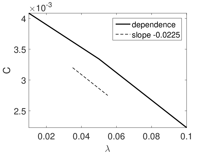
This way, we identify the stability constants
respectively for , , . As the motility of the cell is haptotaxis driven, we correlate through with the corresponding (norm of the) gradients of the ECM
The relation between the stability constant and the gradient of the ECM is approximately linear
| (21) |
see also Figure 6. Clearly, the coefficient might depend on several cellular and extracellular parameters. Nevertheless, it is clearly exhibited by this experiment that the timestep stability constant depends in a linear decreasing way on the gradient of the ECM.
4 Convergence of the FEM
As is typically done in complex models and methods, we exhibit here the convergence of the FEM in characteristic numerical experiments. In particular, we consider chemotaxis, haptotaxis, and chemo-haptotaxis experiments.
In each of these experiments we vary and/or and compute cascades of numerical solutions over nested refined grids. As the exact solutions are not known, we compare every numerical solution to the one of the finest grid.
The experiments that we consider are the following:
Experiment 4.1 (Convergence – Chemotaxis)
The cell migrates over a uniform adhesion substrate, under the influence of a chemical stimulus. The effect of chemotaxis is incorporated as a variable polymerization rate at the membrane. It varies smoothly at the posterior side of the lamellipodium, to at the anterior, see Manhart et al. (2015) for more details. The rest of the parameters are given in Table 3.
Experiment 4.2 (Convergence – Haptotaxis)
The cell migrates within a chemically uniform environment over a non-uniform adhesion substrate. The variable ECM density is included in (6) by the adhesion coefficient,
The polymerization rate is set at the same value22 2 Small changes might occur due to variations in the curvature of the membrane, see Section 2 and Manhart et al. (2015) for details. for all the filaments. The rest of the parameters are set as in Table 3.
 | |
| (a) | (b) |
Experiment 4.3 (Convergence – Chemo-haptotaxis)
For each of the these experiments, the comparison between the results takes place in physical space. We denote by the full cell (area enclosed by the outer border of the lamellipodium) consider the following “norms”:
- Invasiveness:
-
The maximum -coordinate of the cell:
(22a) This “norm” is more suited for experiments where the cell migrates to the right.
- Size:
-
The area of the minimum quadrilateral that the cell occupies:
(22b) - Perimeter:
-
The length of the membrane of the cell, which coincides with the outer boundary of the lamellipodium:
(22c) We compute this “norm” as the length of the closed piecewise-linear curve defined by the outer ends of the discretization filaments.
- Elongation:
-
The ratio of the sides of the minimum quadrilateral that the cell occupies:
(22d)
 | |
| (a) haptotaxis, | (b) chemo-haptotaxis, |
We first define the distance between two cells as
| (23) |
where , , or , represents the “norm” of choice. The convergence results with respect to the and “norms” can be found in Figures 7 – 9; similar results are obtain for the and “norms”.
Figure 7 refers to the chemotaxis Experiment 4.1. We set the fixed value and allow for to vary. For every instance of we compute the “error” as the distance of the corresponding with the one with the finest grid, i.e.
In this case, we deduce a convergence rate of about two. In a similar way, we consider the fixed value and vary to deduce a convergence rate of approximately three.
In Figure 8 we study the convergence of the haptotaxis Experiment 4.2 and the chemo-haptotaxis Experiment 4.3. We set the fixed values and respectively, and allow for to vary. We once again deduce the convergence of the numerical method. When comparing with the convergence in the chemotaxis Experiment 4.1 (shown in Figure 7), the results obtained here indicate that the influence of the non-uniform ECM on the numerical error dissipates fast with respect to the resolution of the grid. In other words, coarse discretization grids are suited better for haptotaxis rather than for chemotaxis experiments.
 |
 |
| inscribed circle diameter | inscribed circle diameter |
| (a) norm | (b) norm |
In Figure 9 we consider again the mixed chemo-haptotaxis Experiment 4.3. This time though, the discretization varies with respect to both and at the same time. As the grid is refined, we consider the diameter of the inscribed circle of the discretization cell as the controlling parameter, and study the convergence of the method with respect to it. We use the norms and , and compare every numerical solution with the one of the finest grid. The detailed results for the “norm” can be found in Table 1, where the convergence rates are computed by the slope of piecewise linear curve.
5 Embedding the FBLM in the extracellular environment
In this section we model and simulate the interactions between the FBLM-FEM and the extracellular environment. We start with a model that describes the extracellular environment and the cell, and with a short description of the numerical method that we use to solve it. We conclude this section with two particular numerical experiments that exhibit the combination of the FBLM-FEM with the environment.
5.1 A model for the environment
We assume that the extracellular environment is comprised of the ECM, a chemical ingredient that serves as chemoattractant for the cell, and matrix metalloproteinases (MMPs) that are secreted by the cell and are responsible for the degradation of the matrix. These environmental components participate in our study via the density of the corresponding (macro-)molecules.
The extracellular chemical, denoted by , is injected in the environment by one or more micro-pipettes that are modelled here as source terms. The chemical is assumed to diffuse freely in the environment, to decay with time (chemical degradation), and to be degraded by the cell upon attachment. The MMPs, denoted by , are produced by the cell, they diffuse freely in the environment, and decay with time. The ECM, denoted by , is assumed to be an immovable component of the system that decays upon attachment of the MMPs, and is not remodelled. Overall the model of the environment reads
| (24) |
with , , and . The number of pipettes is and the corresponding domain/source has support , . The feedback of the FBLM-FEM to the environment takes place through the term , where represents the full cell (lamellipodium and internal structures).
| inscribed circle | convergence | |
|---|---|---|
| diameter | “error” | rate |
| 0.27925 | 0.46966 | — |
| 0.23271 | 0.32897 | 1.9529 |
| 0.19947 | 0.22370 | 2.5022 |
| 0.17453 | 0.18117 | 1.5788 |
| 0.15514 | 0.13964 | 2.2108 |
| 0.13963 | 0.10468 | 2.7357 |
| 0.12693 | 0.08957 | 1.6343 |
| 0.11636 | 0.06306 | 4.0358 |
| 0.10740 | 0.04702 | 3.6627 |
| 0.09973 | 0.03610 | 3.5346 |
Clearly, model (24) is simple and accounts only for some of the basic extracellular processes and interactions between the FBLM and the environment. It can easily be extended to incorporate further and more precise biological properties/phenomena. As it is not though the main aim of this paper, we refrain from such generalizations here and postpone this study for a follow-up work.
As it is easier for the presentation of the numerical method, we write the system (24) in an alternative operator form:
| (25) |
where and where , are the reaction and diffusion operators respectively:
| (26) | ||||
| (27) |
The system (24) (or (25)) is equipped with initial and boundary conditions, and parameters that are experiment specific.
For the numerical treatment of (25) we use a second order Implicit-Explicit Runge-Kutta (IMEX-RK) Finite Volume (FV) numerical method that was previously developed in Kolbe et al. (2016); Sfakianakis et al. (2017) where we refer for more details. Here, in Appendix B, we give some details.
5.2 Coupling the FBLM with the environment

 |
 |

 |
| (a) | (b) | (c) |
The FBLM-FEM (6) and the environment (24) are coupled at three different places through: a) the characteristic function in the model of the environment (24), where the cell produces MMPs and degrades the chemical, b) the adhesion coefficient of the FBLM in (6) that reflects the density of the ECM, see e.g. Experiment 4.2, and c) the polymerization rate in (12) which is primarily controlled by the intensity of the extracellular chemical at the membrane of the cell.
Numerically, the FEM and FV methods that solve the FBLM (6) and environment (24) model, are combined in a modular way. During the time period , , the following hold
- —
The timestep is common in the FEM and the FV and is dictated by the stability of both methods, see also Section (3).
- —
The FV takes into account the position of the cell at , i.e. the FV is explicit with respect to the cell.
- —
Similarly, the FEM is explicit with respect to the density of the ECM and the chemical.
We exhibit the coupling of the cell with the environment, and their interactions with two particular experiments:
Experiment 5.1 (In the environment)
We consider an initial non-uniform adhesion substrate, a circular pipette that injects chemical in the environment, and a rotational symmetric cell in some distance from the pipette. The ECM is given by
| (28) |
where .
The chemical diffuses in the environment and is identified by the cell, which responds with a combined motion to its gradient and to the gradient of the ECM. While the cell migrates, it secretes MMPs that diffuse in the environment, decay, and degrade the ECM.
Experiment 5.1 exhibits the relation between the size of the cell, the width of the lamellipodium, the polymerization rates of the filaments, and the density of the extracellular chemical attractant. We clearly see how the size of the cell increases as it approaches the pipette and the higher density of the chemical, cf. (11) and Manhart et al. (2015); Brunk et al. (2016).
 |
 |
 |

 |
| (a) | (b) | (e) | (e) |
For the next experiment we are motivated by Schlüter and Chaplain (2012); Lo et al. (2000), and in particular by the opposing effects that chemical attraction and the lack of sufficient adhesion can have on the migration of the cell. As the aim of this paper is not to reproduce experimental scenarios, we postpone this more detailed work for a follow-up work. Nevertheless we present it here as an indication of the combination of the FBLM (6) and the environment (24) with multiple chemical sources.
Experiment 5.2 (Adhesion wall)
We consider three sources that inject the same chemical in the environment in a constant rate. The chemical diffuses and decays and a complex chemical landscape is formed in the environment. The ECM exhibits a jump-discontinuity between a higher and lower density that separates the domain in two parts.
| (29) |
The three pipettes reside on the lower-ECM-density part of the domain () whereas an (initially rotational symmetric) cell on the higher-ECM part ().
As the chemical gradient is formed, it is identified by the cell which starts migrating towards the pipettes. The propagating front of the cell ceases further migration when the cell arrives at the discontinuity of the ECM, as it cannot create sufficient adhesions to the lower-density ECM and transfer its momentum. The rest of the cell, that resides on the higher-density ECM, keeps on migrating and the cell effectively elongates in a direction parallel to the discontinuity.
6 Sensitivity analysis
We investigate here the sensitivity of the FBLM-FEM on several of its parameters. We consider a particular experiment and a reference parameter set and compute with them a reference numerical solution. We then vary the parameter set, compute the new results, compare them with the reference solution, and quantify the effect the varied parameters have on the numerical solution.
As opposed to the study of the stability and the convergence in Sections 3 and 4, the sensitivity includes more biological information and meaning. For that reason, we employ now the FBLM augmented with the model for the environment (24).
The control experiment that we consider is a chemotaxis scenario with two sources of chemical.
Experiment 6.1 (Sensitivity – Chemotaxis)
An initially rotational symmetric cell resides over an adhesively uniform substrate
| (30) |
Two sources of the chemical are found in the vicinity of the cell as seen Figure 12 (a). They represent two pipettes of the same circular shape that inject the chemical in the environment with the same rate, cf. Tables 3 and 4 for the relevant parameters.
In Figure 12 we reproduce the time evolution of the Experiment 6.1. As the chemical diffuses in the environment, it decays with time (chemical degradation), and is degraded upon attachment with the cell. The cell responds to the gradient of the chemical by adjusting its polymerization rate, breaking its symmetry, and moving towards the direction of the pipettes.
The parameters we consider in the sensitivity analysis of the FBLM-FEM are
| (31) |
that we index by and set the reference parameter set to be
| (32) |
with values given in Table 3. For this parameter set, the final time conformation of the cell is denoted by and is depicted in Figure 12 (b).
 |
 |
 |
| (a) Initial time | (b) Final time |
We perturb one after the other the reference parameters to new values , while maintaining the rest to their reference values. For each perturbation, the new parameter set differs from the reference set only at the parameter .
For each perturbation of the parameter set, we compute the final time conformation of the cell and compare it with the reference as:
| (33) |
where the “norm” , is one of the “norms” introduced in Section 4. The perturbations of the parameters are small, hence the divided differences in (33) can also be viewed as approximations to the corresponding derivatives, around the reference state .
In essence, represents the rate at which the cell changes, in the sense of the “norm” , with respect to the parameter . Accounting for all the parameters of , the local sensitivity follows. We refer to the Tables and 3 for the full list of the reference parameters and to Table 2 and Figure 13 for a concise description of the sensitivity analysis results.
We note that these results are not global in the sense that they are influenced by the experiment under investigation, the initial state of the cell, the environment, the reference parameters, and more.

|
| (a) Sensitivity results for all the parameters in (31). |

|
| (b) Subtracting the most influential parameters and from (a), reveals the importance of the adhesion coefficient , the inner pulling force , the pressure . |
Nevertheless, we present here some characteristic remarks that will assist in further investigations:
- –
The membrane tethering parameter , is the most influential of the parameters (31) in all the “norms”. The fact in particular that it has a negative effect in the invasiveness “norm” and a positive in the perimeter and elongation “norms”, implies that its primer effect is retractive not on the protruding but rather on the side parts of the cell.
- –
The twisting parameter is equally important. This is in contrast to the lesser influence of the parameter (the other biological component of the crosslink protein). Moreover, the negative influence in area and positive in perimeter “norms” is understood by the fact that the decrease of leads to more linear and radial filaments, and to rotational symmetric and circular cells; hence to (relative) increase of the area and decrease of the perimeter. The decrease of the preferred angle has also the same effect.
- –
All the parameters, except for , have opposite effects in the area and perimeter “norms”. As in the case of , this is understood by the fact that each term either leads towards to or away from a more circular conformation of the cell, which in turn maximizes the area and minimizes the perimeter. In contrast, increase of leads to a larger cell by increasing the inner area of the cell (behind the lamellipodium) and which leads to increase of the total area of the cell and its perimeter.
- –
Increasing the polymerization rates and has a positive effect in all the “norms” except for the perimeter . This is so since the polymerization of filaments opposes the retracting effects of the other components of the model which in turn are responsible for the deformation of the initial rotational symmetric cell; in short: increasing the polymerization rates, leads to more circular cells.
- –
The myosin-actin inner pulling parameter is also very influential in all the “norms”. Note also that and are the only parameters with negative impact in the elongation “norm” . That is, the higher the or the are, the less elongated the cell becomes, see also Figure 11.
- –
We note the effect of and is almost identical in the invasiveness and elongation “norms” , . On the other hand, in the size and elongation “norms” , , their effects are of similar magnitude but opposite sign. This is understood as follows: increase of the adhesion parameter leads to an increase of the size of the cell (see also Brunk et al. (2016)) whereas increase of the stretching parameter leads to its decrease.
| variable | Invasiveness | Area | Perimeter | Elongation |
|---|---|---|---|---|
7 Discussion
The aim of this work was twofold: to investigate two fundamental numerical properties (stability and convergence) of the FEM solving the FBLM, and to embed the FBLM in a complex and adaptive extracellular environment and study its sensitivity to several of its controlling parameters.
We have showed in Section 3 that the FEM exhibits the expected timestep stability behaviour (15) in both chemotaxis and haptotaxis experiments. We have verified this assertion in a particular chemotaxis experiment where we have identified the stability constant and have proposed an automated way of computing proper timesteps for the method. The technique proposed is inspired by the well known ATC methods used in many cases of scientific computing, and is based on the smoothness of the filament polymerization rate and the filament density functions.
We have proceeded further and identified with a series of haptotaxis experiments the dependence between the timestep stability and the gradient of the ECM. We have seen that this relation (21) is linear and we expect it to hold globally, although with different coefficients.
We have exhibited in Section 4 the convergence of the FEM as the discretization grid is refined with respect to and/or . As is commonly done in complex models/methods, we have considered characteristic/representative experimental cases. Since the exact solutions are unknown we deduce the convergence by comparison against the numerical solutions of the finest discretization grid. The comparisons themselves are conducted in terms of particular “norms” that we define in (22a)–(22d).
In Section 5 we have dealt with the embedding of the FBLM-FEM in a complex and adaptive extracellular environment. The model for the environment that we propose in (24) is an reaction-diffusion system of the densities of the involved quantities. The proposed model is relatively simple and is used here mostly to exhibit the coupling between the FBLM and the environment.
We close this work in Section 6 with a first study of the sensitivity of the FBLM-FEM on several of its controlling parameters. This sensitivity analysis is performed around predefined parameter values, most of which are biologically relevant and that have been previously proposed in the literature. We identify the most significant parameters and get an insight on the magnitude of the effect of the different model components.
Although the current work is based on particular experimental cases and is not escorted by rigorous numerical (or other type of) analysis, the benefit is twofold:
On the one hand, the combination FBLM-FEM can be further used to model and simulate biologically relevant experimental situations. We know now that the refinement of the discretization grid, augmented by the automated adaptation of the timestep, provides with a stable and converging method that will reveal the inherent dynamics of the model.
On the other hand, having verified that the behaviour of the FBLM-FEM is the expected one in terms of convergence and stability, the rigorous numerical analysis is well warranted. It is expected that the remarks of this work will serve also as a guide in this effort.
Moreover, the coupling of the FBLM with the extracellular environment that we propose here will serve as springboard for the further modelling and simulation of more biologically relevant settings and in-vitro experiments. It can easily be extended to include e.g. the description of the ECM as a fibrous component of the environment, more than one chemical ingredients (attractants or repellents), as well as more than one cells interacting with each other.
The sensitivity analysis results have served here for the deeper understanding of the effect of different terms on the model. The insight we have gained will serve in the further refinement of the FBLM-FEM and the parameter estimation procedures, when reproducing and simulating realistic experimental scenarios.
| symb. | description | value | comment |
|---|---|---|---|
| bending elasticity | Gittes et al. (1993) | ||
| adhesion | Li et al. (2003); Oberhauser et al. (2002) & Oelz et al. (2008); Oelz and Schmeiser (2010a); Oelz and Schmeiser (2010b) | ||
| cross-link twisting | |||
| cross-link stretching | |||
| crosslinker equil. angle | Oelz and Schmeiser (2010b) | ||
| actin-myosin strength | |||
| minimal polymerization | in biological range | ||
| maximal polymerization | in biological range | ||
| pressure constant | |||
| equilibrium inner area | Verkhovsky et al. (1999); Small et al. (1978) | ||
| inextensibility | |||
| membrane tethering |
| symb. | description | Experiment 5.1 | Experiment 5.2 | Experiment 6.1 |
|---|---|---|---|---|
| and Figure 10 | and Figure 11 | and Figure 12 | ||
| diffusion of the chemical | ||||
| diffusion of the MMPs | ||||
| production rate of chemical | ||||
| production of MMPs | ||||
| decay of the chemical | ||||
| decay of the MMPs | ||||
| degr. chemical by the cell | ||||
| degr. of the ECM by the MMPs |
Acknowledgement
The authors would like to thank Christian Schmeiser, Anna Marciniak-Czochra, and Mark Chaplain for the fruitful discussions and suggestions during the preparation of this manuscript.
References
- Small et al. [2002] J.V. Small, T. Stradal, E. Vignal, and K. Rottner. The lamellipodium: where motility begins. Trends Cell Biol., 12(3):112–20, 2002.
- Svitkina et al. [1997] T.M. Svitkina, A.B. Verkhovsky, K.M. McQuade, and G.G. Borisy. Analysis of the actin-myosin II system in fish epidermal keratocytes: mechanism of cell body translocation. J. Cell Biol., 139(2):397–415, 1997.
- Yam et al. [2007] P.T. Yam, C.A. Wilson, L. Ji, B. Herbert, E.L. Barnhart, N.A. Dye, P.W. Wiseman, G. Danuser, and J.A. Theriot. Actin-myosin network reorganisation breaks symmetry at the cell rear to sponaneously initiate polarized cell motility. J. Cell Biol., 178(7):1207–1221, 2007.
- Postlethwaite and Keski-Oja [1987] A.E. Postlethwaite and J. Keski-Oja. Stimulation of the chemotactic migration of human fibroblasts by transforming growth factor beta. J. Exper. Med., 165(1):251–256, 1987.
- Gerisch and Keller [1981] G. Gerisch and H.U. Keller. Chemotactic reorientation of granulocytes stimulated with micropipettes containing fMet-Leu-Phe. J. Cell Sci., 52:1–10, 1981.
- Iijima et al. [2002] M. Iijima, Y. E. Huang, and J. Devreotes. Temporal and spatial regulation of chemotaxis. Dev. Cell, 3(4):469–478, 2002.
- Zigmond and Hirsch [1973] S.H. Zigmond and J.G. Hirsch. Leukocyte locomotion and chemotaxis. J. Exper. Med., 137:387–410, 1973.
- [8] L. Blanchoin, R. Boujemaa-Paterski, C. Sykes, and J. Plastino. Actin dynamics, architecture, and mechanics in cell motility. Physiol. Rev.
- Lauffenburger and Horwitz [1996] D.A. Lauffenburger and A.F. Horwitz. Cell migration: a physically integrated molecular process. Cell, 84(3):359–69, 1996. ISSN 0092-8674.
- Gittes et al. [1993] F. Gittes, B. Mickey, J. Nettleton, and J. Howard. Flexural rigidity of microtubules and actin filaments measured from thermal fluctuations in shape. J. Cell Biol., 120(4):923–34, 1993. ISSN 0021-9525.
- Tojkander et al. [2012] S. Tojkander, G. Gateva, and P. Lappalainen. Actin stress fibers - assembly, dynamics and biological roles. J. Cell Sci., 125(8):1855–1864, 2012.
- Mitchison and Cramer [1996] T.J. Mitchison and L.P. Cramer. Actin-based cell motility and cell locomotion. Cell, 84(3):371–379, 1996.
- Jay et al. [1995] P.Y. Jay, P.A. Pham, S.A. Wong, and E.L. Elson. A mechanical function of myosin II in cell motility. J. Cell Sci., 108(1):387–393, 1995.
- Chen [1981] W.T. Chen. Mechanism of retraction of the trailing edge during fibroblast movement. The Journal of Cell Biology, 90(1):187–200, 1981.
- Sabass and Schwarz [2010] B. Sabass and U.S. Schwarz. Modeling cytoskeletal flow over adhesion sites: competition between stochastic bond dynamics and intracellular relaxation. J. Phys.: Condens. Matter, 22:194112 (10pp), 2010.
- Fuhrmann and Stevens [2015] J. Fuhrmann and A. Stevens. A free boundary problem for cell motion. Diff. Integr. Eq., 28:695–732, 2015.
- Marth et al. [2015] W. Marth, S. Praetorius, and A. Voigt. A mechanism for cell motility by active polar gels. J. R. Soc. Interface, 12:20150161, 2015.
- Rubinstein et al. [2009] B. Rubinstein, M.F. Fournier, K. Jacobson, A.B. Verkhovsky, and A. Mogilner. Actin-myosin viscoelastic flow in the keratocyte lamellipod. Biophys. J., 97(7):1853–1863, 2009.
- Alt and Kuusela [2009] W. Alt and E. Kuusela. Continuum model of cell adhesion and migration. J. Math. Biol., 58(1-2)::135, 2009.
- Cardamone et al. [2011] L. Cardamone, A. Laio, V. Torre, R. Shahapure, and A. DeSimone. Cytoskeletal actin networks in motile cells are critically self-organized systems synchronized by mechanical interactions. PNAS, 108:13978–13983, 2011.
- Scianna et al. [2013] M. Scianna, L. Preziosi, and K. Wolf. A cellular potts model simulating cell migration on and in matrix environments. Math. Biosci. Engng., 10:235–261, 2013.
- Möhl et al. [2012] C. Möhl, N. Kirchgessner, C. Schäfer, B. Hoffmann, and R. Merkel. Quantitative mapping of averaged focal adhesion dynamics in migrating cells by shape normalization. J. Cell Sci., 125:155–165, 2012.
- Madzvamuse and George [2013] A. Madzvamuse and U.Z. George. The moving grid finite element method applied to cell movement and deformation. Finite Elem. Anal. Des., 74:76 – 92, 2013.
- Ambrosi and Zanzottera [2016] D. Ambrosi and A. Zanzottera. Mechanics and polarity in cell motility. Physica D, 330:58–66, 2016.
- Oelz et al. [2008] D. Oelz, C. Schmeiser, and J.V. Small. Modeling of the actin-cytoskeleton in symmetric lamellipodial fragments. Cell Adhes. Migr., 2:117–126, 2008.
- Oelz and Schmeiser [2010a] D. Oelz and C. Schmeiser. Derivation of a model for symmetric lamellipodia with instantaneous cross-link turnover. Arch. Ration. Mech. An., 198:963–980, 2010a.
- Manhart et al. [2015] A. Manhart, D. Oelz, C. Schmeiser, and N. Sfakianakis. An extended Filament Based Lamellipodium: Model produces various moving cell shapes in the presence of chemotactic signals. J. Theor. Biol., 382:244–258, 2015.
- Manhart et al. [2016] A. Manhart, D. Oelz, C. Schmeiser, and N. Sfakianakis. Numerical treatment of the Filament Based Lamellipodium Model (FBLM). Book chapter in Modelling Cellular Systems, 2016.
- Brunk et al. [2016] A. Brunk, N. Kolbe, and N. Sfakianakis. Chemotaxis and haptotaxis on a cellular level. Proc. XVI Int. Conf. Hyper. Prob., 2016.
- Oelz and Schmeiser [2010b] D. Oelz and C. Schmeiser. Cell mechanics: from single scale-based models to multiscale modeling, chapter How do cells move? Mathematical modeling of cytoskeleton dynamics and cell migration. Chapman and Hall, 2010b.
- Hundsdorfer and Verwer [2003] W. Hundsdorfer and J. Verwer. Numerical solution of time-dependent advection-diffusion-reaction equations. Springer Series in Computational Mathematics, Springer-Verlag, Berlin, 2003.
- [32] R. LeVeque. Finite Volume Methods for Hyperbolic Problems. Cambridge University Press.
- Kolbe et al. [2016] N. Kolbe, J. Katuchova, N. Sfakianakis, Hellmann N., and M. Lukacova-Medvidova. A study on time discretization and adaptive mesh refinement methods for the simulation of cancer invasion: The urokinase model. Appl. Math. Comput., 273:353–376, 2016.
- Shu [2009] C.W. Shu. High order weighted essentially non-oscillatory schemes for convection dominated problems. SIAM Review, 51:82–126, 2009.
- Sfakianakis et al. [2017] N. Sfakianakis, N. Kolbe, Hellmann N., and M. Lukacova-Medvidova. A multiscale approach to the migration of cancer stem cells: Mathematical modelling and simulations. Bull. Math. Biol., 79:209–235, 2017.
- Schlüter and Chaplain [2012] I. Schlüter, D.K. Ramis-Conde and M.A. Chaplain. Computational modeling of single-cell migration: the leading role of extracellular matrix fibers. J. Biophys., 103(6):1141–51, 2012.
- Lo et al. [2000] C.M. Lo, H.B. Wang, M. Dembo, and Y.L. Wang. Cell movement is guided by the rigidity of the substrate. J. Biophys., 79(1):144–152, 2000.
- Li et al. [2003] F. Li, S.D. Redick, H.P. Erickson, and V.T. Moy. Force measurements of the integrin-fibronectin interaction. Biophys. J., 84(2):1252–1262, 2003.
- Oberhauser et al. [2002] A.F. Oberhauser, C. Badilla-Fernandez, M. Carrion-Vazquez, and J.M. Fernandez. The mechanical hierarchies of fibronectin observed with single-molecule AFM. J. Mol. Biol., 319(2):433–47, 2002.
- Verkhovsky et al. [1999] A.B. Verkhovsky, T.M. Svitkina, and G.G. Borisy. Self-polarisation and directional motility of cytoplasm. Curr. Biol., 9(1):11–20, 1999.
- Small et al. [1978] J.V. Small, G. Isenberg, and J.E. Celis. Polarity of actin at the leading edge of cultured cells. Nature, bf 272:638–639, 1978.
- Kennedy and Carpenter [2003] C.A. Kennedy and M.H. Carpenter. Additive Runge-Kutta schemes for convection-diffusion-reaction equations. Appl. Numer. Math., 1(44):139–181, 2003.
- Krylov [1931] A.N. Krylov. On the numerical solution of the equation by which in technical questions frequencies of small oscillations of material systems are determined. Otdel. mat. i estest. nauk., VII(4):491–539, 1931.
- van der Vorst [1992] H.A. van der Vorst. Bi-CGSTAB: A fast and smoothly converging variant of Bi-CG for the solution of nonsymmetric linear systems. SIAM J. Sci. Comput., 13(2):631–644, 1992.
Appendix A The FEM for the FBLM
We numerically solve the FBLM (6) with a problem specific FEM that was first presented in Manhart et al. [2016]. Here we present some of its components.
The maximal filament length varies around the lamellipodium, and in effect the computational domain
is non-rectangular. For consistency and stability reasons we recover the orthogonality of the domain , using the coordinate transformation
and replace it by
| (34) |
Accordingly, the weak formulation of (6), recasts into
| (35) |
with . In a similar manner the modified material derivative and in-extensibility conditions read
and
We decompose into disjoined rectangular computational cells as follows:
| (36) |
for , , , and , , . The resolution of the grid along the and directions is denoted by , . The -periodicity assumption suggests that is identified with .
We follow Manhart et al. [2016] and set the conforming FE space
| (37) |
of continuous functions that are continuously differentiable with respect to , and such that on each computational cell they coincide with a first order polynomial in , and a third order polynomial in .
In particular, we consider for , , and , that
| (38) |
with
| (39) |
and that , , whenever .The basis functions are then defined as:
| (40) |
for , and the element can be represented in terms of the point values and the -derivatives at the discretization nodes, as:
| (41) |
The FE formulation of the lamellipodium problem on the time interval is to find , such that (35) holds for all .
Appendix B The FV method the environment
We solve the (24) using a FV method that was previously developed in Kolbe et al. [2016], Sfakianakis et al. [2017] where we refer for details. Here we provide some information.
We consider the advection-reaction-diffusion (ARD) system
| (42) |
where represents the solution vector, and , , and the advection, reaction, and diffusion operators respectively.
We denote by the corresponding (semi-)discrete numerical approximation, indexed by the maximal diameter of the spatial grid , that satisfies the system of ODEs
| (43) |
where the numerical operators , , and are discrete approximations of the operators , , and in (42) respectively.
We split (43) in an explicit and an implicit part as
| (44) |
The details of the splitting depend on the particular problem in hand but in a typical case, the advection terms are explicit in time, the diffusion terms implicit, and the reaction terms partly explicit and partly implicit, according to the reaction rates.
More precisely, we employ a diagonally implicit RK method for the implicit part, and an explicit RK for the explicit part
| (45) |
where are the stages of the IMEX method, , , , , are respectively the coefficients for the explicit and the implicit part of the scheme, given in the Butcher Tableau in Table 5, Kennedy and Carpenter [2003]. The linear systems in (45) are solved using the iterative biconjugate gradient stabilized Krylov subspace method Krylov [1931], van der Vorst [1992].
| 0 | ||||