Graph-Theoretic Framework for Unified Analysis of Observability and Data Injection Attacks in the Smart GridThanks: This research was supported by the U.S. National Science Foundation under Grants ECCS-1549894 and CNS-1446621, and in part by the Office of Naval Research (ONR) MURI Grant N00014-16-1-2710.

In this regard, the works in [10] and [11] focused on computing a security set which comprises the minimum set of measurements which must be attacked in addition to a certain specific measurement in order to make the system unobservable. Moreover, the work in [12] focused on computing the cardinality of the smallest set of meters which when attacked render the system unobservable. The authors in [13, 14, 15] extended such observability problems to studying SDIAs. In this regard, these works focused on characterizing the sparsest stealthy attack containing a certain specific measurement. In addition, the work in [16] focused on characterizing a set of measurements to defend so that no attack which concurrently manipulates a set of meters whose cardinality is below a certain threshold can be stealthy. Hence, this latter analysis focuses on the defense against resource-limited attackers. As such, these works have focused on formulating and studying mathematical problems whose solutions enable anticipating potential sophisticated attacks – which constitutes a first step towards deriving corresponding defense mechanisms – and designing optimal defense strategies to thwart such attacks and mitigate their potential effect.

The computational complexity of these problems [10, 11, 12, 13, 14, 15, 16] has led to limiting the analysis of their solutions to special, often approximated, cases or required the use of heuristics and relaxation techniques which led to suboptimal solutions. For example, for characterizing the sparsest observability attacks containing a specific measurement, the work in [10] focused on the special case of measurement sets of low cardinality while the work in [11] derived an approximate solution that is based on the solution of a min-cut problem. In addition, with regard to the analysis of the sparsest SDIAs containing a certain measurement [13, 14, 15], the work in [13] focused on deriving an upper-bound on this stealthy attack set while the work in [14] used min-cut relaxation techniques to approximate the sought solution. Moreover, the work in [15] proposed a heuristic algorithm which can approximate the solution of the studied problem while an exact solution was found for the special case in which power flows over all the transmission lines and power injections into and out of every bus are assumed to be measured. To defend against a resource-limited data injection attacker, the authors in [16] used an $l_{1}$ relaxation method for characterizing the set of meters to defend to thwart SDIAs launched by attackers whose attack space is limited by a certain cardinality threshold. Other related security works are also found in [17, 18, 19, 20, 21, 22].

Therefore, this rich body of literature [10, 11, 12, 13, 14, 15, 16, 17, 18, 19, 20, 21, 22] employs heuristics and approximation techniques to numerically approximate the solutions to these fundamental observability attacks and SDIA problems rather than propose new analytical methods for studying these problems and characterizing their solutions. As such, there is a need for an analytical framework which allows modeling and studying such data availability and integrity attacks and enables an analytical characterization of solutions to such widely-studied security problems. In addition, the fact that these works [10, 11, 12, 13, 14, 15, 16] studied correlated problems but from different perspectives highlights the need for a unified framework using which solutions to such correlated observability attacks and SDIA problems can be studied and derived.

The main contribution of this paper is a novel unified graph-theoretic framework that enables a global detailed modeling and understanding of observability attacks and SDIAs. As a result, this framework provides a unified tool for analyzing various widely-studied observability attacks and SDIA problems such as those studied in [10, 11, 12, 13, 14, 15, 16], among others. In addition, the proposed framework enables a graph-theoretic characterization of solutions to such security problems. In this regard, our proposed framework is based on a shift in the modeling of observability attacks and SDIAs from a linear algebra frame of reference to a graph-theoretic perspective. As a result, based on this proposed framework, such attacks can be modeled and analyzed by requiring only power system topological data, namely, the power system 1-line diagram and the location of deployed measurement units without the need for neither line parameters data nor the exact knowledge of power flow levels throughout the system.

To build the proposed framework, we first begin by introducing a graph-theoretic basis of observability attacks and, then, we prove that SDIAs are a special case of such observability attacks. In this respect, we introduce an algorithm providing a step-by-step approach for building critical sets, a set of measurements – containing a certain specific measurement – which, when removed, renders the system unobservable. We then prove that for a DIA to be stealthy, the attacked measurements should strictly result in leaving critical sets unmatched as part of a maximum matching over an introduced bipartite graph. As such, a graph-theoretic model of SDIAs is then introduced based on which we analyze various well-studied SDIA problems. In particular, we show that our developed framework enables a graph-theoretic characterization of solutions to various SDIA problems such as, but not limited to: 1) Finding the stealthy attack of lowest cardinality, 2) Finding the stealthy attack of lowest cardinality, including a specific measurement, 3) Finding a set of measurements which when defended can thwart all possible stealthy attacks, and 4) Finding a set of measurements to defend against a resource-limited attacker, among others. Here, we note that our goal is not to propose tractable algorithms to these problems, but rather to identify graph-theoretic problems whose solutions would lead to the solutions of these problems. A case study using the IEEE 14-bus system, with $17$ distributed measurement units, is considered throughout the paper to showcase the developed analytical concepts.

The rest of the paper is organized as follows. Section II introduces state estimation and power system observability. Section III introduces our proposed graph-theoretic foundation of observability attacks and shows its impact on modeling and analyzing such data availability attacks. Section IV introduces the proposed graph-theoretic framework for modeling SDIAs, as well as investigates various well-studied SDIA problems. Section V concludes the paper and provides an outlook detailing the impact of the proposed framework on studying future observability and data injection attacks.

A summary of the main notations used in this paper is given in Table I.

Consider a power system state estimation process which uses various measurements collected from across the system to estimate the voltage magnitudes and phase angles at every bus in the system, known as the system states [8]. Let $\boldsymbol{z}\in\mathds{R}^{\mu}$ ($\mu$ being the number of measurements) be the vector of collected measurements, which includes power flow levels (real and reactive) over transmission lines, power (real and reactive) injected in or withdrawn from certain buses, as well as bus voltage magnitudes. In addition, let $\boldsymbol{x}\in\mathds{R}^{\nu}$ be the vector of system states. The relationship between the measurements and the states directly follows from the linearized power flow equations [8]:

where $\boldsymbol{H}\in\mathds{R}^{\mu\times\nu}$ is the measurement Jacobian matrix and $\boldsymbol{e}\in\mathds{R}^{\mu}$ is the vector of random errors that typically follows a Gaussian distribution, ${N(0,\boldsymbol{R})}$, where $\boldsymbol{R}$ is positive definite. Here $\mu\geq\nu$, that is the dimension of $\boldsymbol{x}$ cannot be larger than the dimension of the measurement vector, $\boldsymbol{z}$. Further, we assume that $\boldsymbol{H}$ is a full column rank matrix. Using a maximum-likelihood estimator – a weighted least squares estimator (WLS) for a Gaussian error vector $\boldsymbol{e}$ – an estimate of the states, $\hat{\boldsymbol{x}}$, will be:

This estimate of all the states provides visibility of the steady-state operating conditions of the system, based on which various operational decisions are performed [8].

The observability¹¹ 1 Our analysis focuses on static state estimation and static observability of the power system, which is a fundamental aspect of power system analysis [8]. Our analysis, thus, does not extend to dynamic observability of a power system, which would arise with dynamically changing states. of the power system consists of the ability to uniquely determine its states based on the collected set of measurements [8]. Observability, hence, requires the collected measurements to provide a sufficient number of independent equations to allow for the estimation of the state vector, $\boldsymbol{x}$. Otherwise, when this observability condition is not met, the power system is dubbed unobservable. The power system is observable if and only if the measurement matrix $\boldsymbol{H}$ is of full column rank [8], which was our initial assumption. This is known as algebraic observability, as it enables assessment of observability using linear algebra. Due to the $P-\theta$, $Q-V$ decoupling²² 2 $P$ denotes real power, $\theta$ denotes voltage phase angles, $Q$ denotes reactive power, and $V$ denotes voltage magnitudes. in power systems [9], the observability analysis can be decoupled by separately studying the observability of voltage phase angles, using real power measurements, and the observability of voltage magnitudes, based on reactive power measurements. Since the two analyses are identical, we focus here on phase angle observability. To this end, we consider $\boldsymbol{z}\in\mathds{R}^{\mu}$ to be a vector of real power measurements (bus injections and line flows), and the state vector $\boldsymbol{x}\in[-\pi,\pi]^{\nu}$ to be the vector of voltage phase angles (in radians). Here, $\nu=N-1$ for a power system with $N$ buses given that the phase angle of the reference bus is fixed and is taken to be the reference with respect to which all other phase angles are calculated [8].

An alternative measure of observability, which turns out to be equivalent to algebraic observability, has been proposed in [23] and uses graph-theoretic techniques to introduce the concept of topological observability. Topological observability is equivalent to algebraic observability, in the sense that it enables assessment of the observability of the power system using graph-theoretic tools rather than using linear algebra as done for algebraic observability. In this regard, let the power system 1-line diagram be represented as a graph $\mathcal{G}(\mathcal{N},\mathcal{L})$ in which the set of vertices $\mathcal{N}$, $|\mathcal{N}|=N$, represents the set of buses of the power system while the set of branches $\mathcal{L}$, $|\mathcal{L}|=L$, represents the set of lines. One key result that was shown in [23] and that will be of relevance to our work is the following:

If a measurement assignment yields a spanning tree over the power network $\mathcal{G}$, then the power system will be observable (and vice versa). Fig. 1 shows an example of measurement assignments over the IEEE 14-bus system. This figure shows the tree edges (marked in solid red lines) to which measurement where assigned as part of the measurement assignment function. The measurements that were assigned to each one of these edges are identified using dashed arrow lines originating from the assigned measurement and pointing to the line to which this measurement is assigned. This tree is formed of edges $\{1,\,2,\,4,\,6,\,8,\,9,\,10,\,12,\,13,\,15,\,16,\,17,\,19\}$ and spans the whole vertex set $\mathcal{N}$ of the power system graph $\mathcal{G}$, and hence, is a spanning tree. As a result, since this measurement assignment yields a spanning tree, then the available set of measurements renders the system observable.

Let $\mathcal{M}$ be the set of measurements, and let $\mathcal{T}(\mathcal{N},\mathcal{B})$ be a spanning tree formed by an assignment of a subset of measurements, $\mathcal{M}^{A}\subseteq\mathcal{M}$, to a subset of lines $\mathcal{B}\subseteq\mathcal{L}$ following the measurement assignment rules in Proposition 1. The assignment of measurements in $\mathcal{M}^{A}$ to lines in $\mathcal{B}$ for constructing the spanning tree $\mathcal{T}(\mathcal{N},\mathcal{B})$ can be modeled by an assignment function $f(.)$ formally defined [23] as follows:

For example, in Fig. 1, $\mathcal{M}^{A}$ is composed of the injection measurements over buses $1,2,3,5,6,9$, and $13$ and the line flow measurements over lines $2,8,9,15,17$, and $19$. In addition, $\mathcal{B}=\{1,\,2,\,4,\,6,\,8,\,9,\,10,\,12,\,13,\,15,\,16,\,17,\,19\}$, where each edge of $\mathcal{B}$ in Fig. 1 is colored in red. Moreover, the corresponding assignment function $f(.)$ is visualized in Fig. 1 by dashed red arrows indicating which measurement in $\mathcal{M}^{A}$ is assigned to which line in $\mathcal{B}$.

Measurements in $\mathcal{M}$ that are not part of $\mathcal{M}^{A}$, i.e. $m\in\mathcal{M}\setminus{\mathcal{M}^{A}}$, are not assigned measurements and are, therefore, redundant measurements with respect to the assigned set of measurements $\mathcal{M}^{A}$. Here, we note that due to this redundancy, a spanning tree which can be obtained from the measurement set following the measurement assignment rules may not be unique [23]. Hence, when such a redundancy exists, following a different assignment function can result in a different spanning tree and, hence, in different sets of assigned and redundant measurements.

Various algorithms of low complexity have been proposed to find and build such a spanning tree [23, 24, 25]. In this regard, the work in [23] proposes an algorithm to find a spanning tree over $\mathcal{G}$, which will be used in some of the derivations in the following sections. This algorithm starts by processing flow measurements by assigning each flow measurement to its corresponding branch to form disjoint tree components. Then, injection measurements are assigned to lines in a way to connect these tree components to form one spanning tree. Here, we highlight one type of injection measurements, namely, boundary injections, which will play a crucial role in our derivations.

Boundary injections play a major role in connecting these tree components. Indeed, for a bus which is not incident to a measured line to be connected to the spanning tree, it has to be reachable from a boundary injection through a series of measurement assignments [23]. As such, boundary injections are considered to be sources and unmeasured buses are considered to be sinks which must be connected to these sources following the set of measurement assignment rules.

We next build on the foundation of topological observability to present a graph-theoretic framework for modeling and studying the security of the smart grid facing observability attacks and SDIAs. This framework is based on our proposed concepts of critical sets and observability sets, which we define and derive in the next section.

Understanding and modeling observability attacks requires an in-depth understanding of the effect of the loss of any bundle of measurements on the observability of the system. In this regard, we next introduce a structured method for identifying, for each measurement $m$, a minimal set of measurements including $m$ (which we refer to as a critical set of $m$), which when removed renders the system unobservable. To this end, we first characterize the set of potential measurements to be investigated, for each measurement $m$, and then provide the necessary discussion and introduce the underlying method for characterizing a critical set of $m$. Then, a detailed algorithm is introduced to provide a step-by-step method for characterizing such critical sets.

As defined in Section II-B, we let $\mathcal{M}^{A}\subseteq\mathcal{M}$ be a set of assigned measurements, i.e., a subset of measurements that are assigned to a subset of lines of the power system graph $\mathcal{G}(\mathcal{N},\mathcal{L})$, following the measurement assignment rules in Proposition 1, to form a spanning tree, $\mathcal{T}(\mathcal{N},\mathcal{B})$, over this graph. As described in Section II-B, $\mathcal{T}(\mathcal{N},\mathcal{B})$ is a spanning tree as it includes all the nodes of $\mathcal{G}(\mathcal{N},\mathcal{L})$. The set of edges of this tree, i.e. $\mathcal{B}$, represents the set of lines to which measurements in $\mathcal{M}^{A}$ were assigned to construct the spanning tree. We refer to measurements that are not part of $\mathcal{M}^{A}$ as unassigned measurements. We consider that the system is originally observable. Hence, such a spanning tree and its corresponding set of assigned measurements exist.

In this regard, consider a spanning tree $\mathcal{T}(\mathcal{N},\mathcal{B})$ resulting from a measurement assignment and consider an assigned measurement $m\in\mathcal{M}^{A}$. Since $m$ is assigned to a line $f(m)$ to build the spanning tree $\mathcal{T}(\mathcal{N},\mathcal{B})$, its removal will split the original tree $\mathcal{T}(\mathcal{N},\mathcal{B})$ into two trees $\mathcal{T}_{1}^{m}(\mathcal{N}^{m}_{1},\mathcal{B}_{1}^{m})$ and $\mathcal{T}_{2}^{m}(\mathcal{N}_{2}^{m},\mathcal{B}_{2}^{m})$ each spanning, respectively, subgraphs $\mathcal{G}^{m}_{1}(\mathcal{N}^{m}_{1},\mathcal{L}^{m}_{1})$ and $\mathcal{G}^{m}_{2}(\mathcal{N}^{m}_{2},\mathcal{L}^{m}_{2})$, such that $\mathcal{N}=\mathcal{N}^{m}_{1}\cup\mathcal{N}^{m}_{2}$ and $\mathcal{B}=\mathcal{B}^{m}_{1}\,\cup\,\mathcal{B}_{2}^{m}\,\cup\,\{f(m)\}$. We let $N^{m}_{1}=|\mathcal{N}^{m}_{1}|$ and $N^{m}_{2}=|\mathcal{N}^{m}_{2}|$. We refer to the set of measurements within each of $\mathcal{G}^{m}_{1}(\mathcal{N}^{m}_{1},\mathcal{L}^{m}_{1})$ and $\mathcal{G}^{m}_{2}(\mathcal{N}^{m}_{2},\mathcal{L}^{m}_{2})$ by, respectively, $\mathcal{M}^{m}_{1}$ and $\mathcal{M}^{m}_{2}$. In other words, $\mathcal{M}^{m}_{i}$, for $i\in\{1,2\}$, consists of injection measurements over buses in $\mathcal{N}^{m}_{i}$ and power flow measurements over lines in $\mathcal{L}^{m}_{i}$.

Fig. 2 provides an illustrative example of the two spanning trees created by the deletion of flow measurement $F_{2}$ over line $2$. Here, $f(F_{2})$ is line $2$. Fig. 2 represents the same system shown in Fig. 1 and will be used hereinafter to provide a practical example of the defined concepts and analytical derivations. As can be seen from Fig. 2, since $F_{2}$ was assigned to line $2$, when the measurement assignment is not modified (i.e. not considering the redundant measurements), the removal of $F_{2}$ will split the original tree $\mathcal{T}(\mathcal{N},\mathcal{B})$, represented in solid red lines in Fig. 1, into two trees each of which spans a subgraph of $\mathcal{G}(\mathcal{N},\mathcal{B})$, namely, subgraphs $\mathcal{G}^{F_{2}}_{1}$ and $\mathcal{G}^{F_{2}}_{2}$ in Fig. 2.

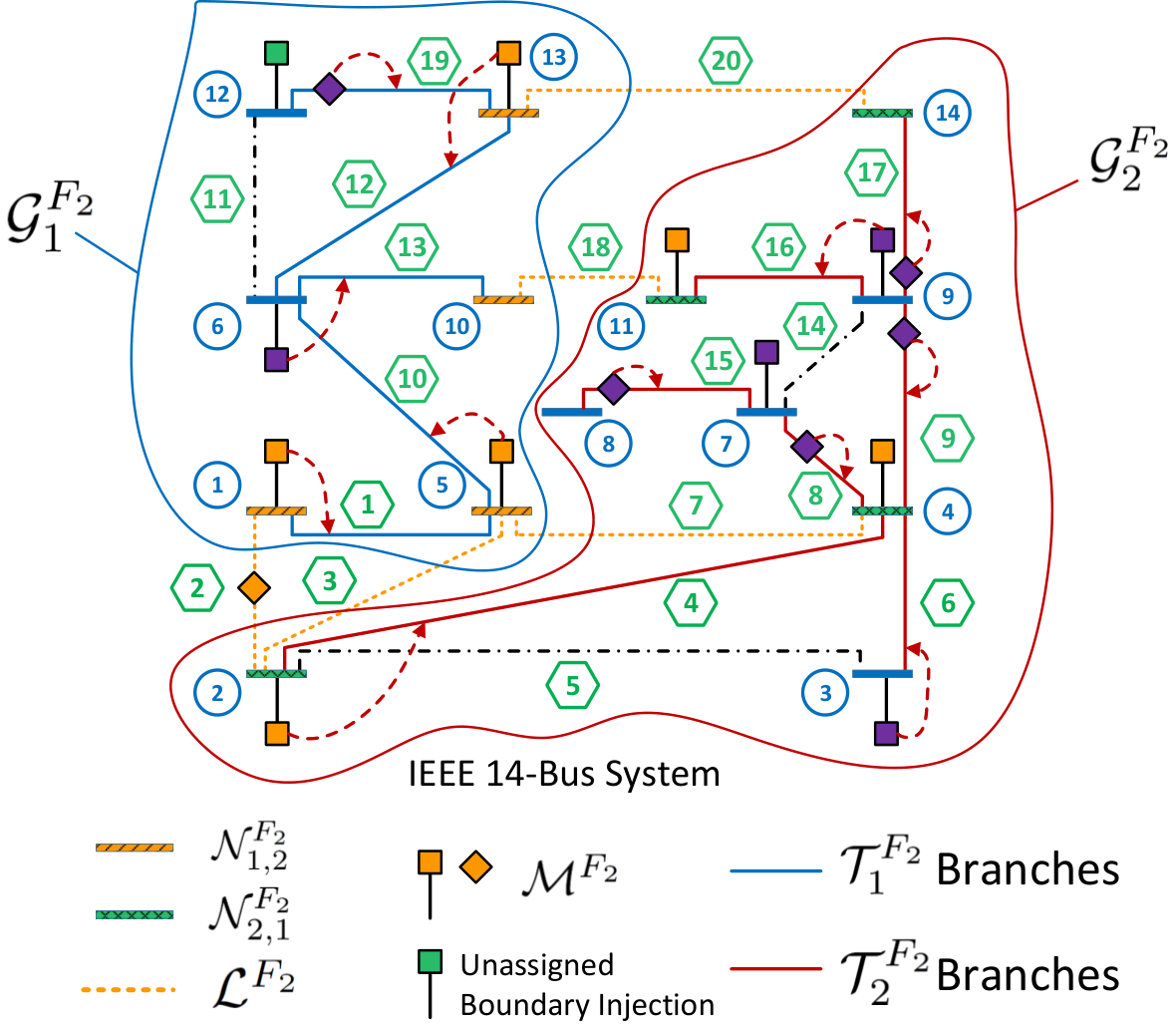
We let $\mathcal{L}^{m}$ be the set of lines connecting a bus in $\mathcal{G}_{1}^{m}$ to a bus in $\mathcal{G}_{2}^{m}$. In addition, let $\mathcal{N}_{1,2}^{m}\subseteq\mathcal{N}_{1}^{m}$ and $\mathcal{N}_{2,1}^{m}\subseteq\mathcal{N}_{2}^{m}$ be the set of nodes in, respectively, $\mathcal{N}_{1}^{m}$ and $\mathcal{N}_{2}^{m}$ which are connected to a node in, respectively, $\mathcal{N}_{2}^{m}$ and $\mathcal{N}_{1}^{m}$. An example of these notations is provided in Fig. 2, for $m\triangleq F_{2}$. $\mathcal{L}^{m}$ is, hence, formally defined as:

$\mathcal{G}_{1}^{m}$ and $\mathcal{G}_{2}^{m}$ are two disjoint subgraphs of $\mathcal{G}$. Hence, for any tree to potentially span $\mathcal{G}$, it must connect $\mathcal{G}_{1}^{m}$ and $\mathcal{G}_{2}^{m}$ (i.e. connect at least one node of $\mathcal{G}_{1}^{m}$ to a node in $\mathcal{G}_{2}^{m}$), which can only be achieved by assigning a measurement to a line in $\mathcal{L}^{m}$. In this regard, we define $\mathcal{M}_{\mathcal{L}^{m}}$ to be the set of line measurements over lines in $\mathcal{L}^{m}$ and injection measurements over buses incident to $\mathcal{L}^{m}$, i.e., buses in $\{\mathcal{N}_{1,2}^{m}\,\cup\,\mathcal{N}_{2,1}^{m}\}$. Based on the measurement assignment rules described in Section II-B, also summarized in Proposition 1, only measurements in $\mathcal{M}_{\mathcal{L}^{m}}$ could be potentially assigned to a line in $\mathcal{L}^{m}$. As a result, removing all of the measurements in $\mathcal{M}_{\mathcal{L}^{m}}$ will guarantee that the system becomes unobservable, as it guarantees that two subgraphs of $\mathcal{G}$ would never be connected by any measurement assignment, making it, thus, impossible to build a spanning tree over $\mathcal{G}$. Hence, the removal of $\mathcal{M}_{\mathcal{L}^{m}}$ is a sufficient condition for causing the unobservability of the system. However, removing the entire set $\mathcal{M}_{\mathcal{L}^{m}}$ may be more than required to prevent any possible measurement assignment (or constructed tree) from connecting $\mathcal{G}_{1}^{m}$ and $\mathcal{G}_{2}^{m}$; a goal which could be achieved by the removal of only a subset of $\mathcal{M}_{\mathcal{L}^{m}}$, as we investigate next.

In this regard, for the pair of subgraphs $\mathcal{G}_{1}^{m}$ and $\mathcal{G}_{2}^{m}$, resulting from the spanning tree $\mathcal{T}$, we define a set of measurements, $\mathcal{C}^{m}\in\mathcal{M}_{\mathcal{L}^{m}}$, for each measurement $m\in\mathcal{M}^{A}$, to which we refer as a critical set of $m$, as follows:

In other words, $\mathcal{C}^{m}$ includes $m$ and a maximal set of redundant measurements in $\mathcal{M}_{\mathcal{L}^{m}}\setminus\{m\}$. When all of the measurements within $\mathcal{C}^{m}$ except for an arbitrary one are removed, $\mathcal{G}_{1}^{m}$ and $\mathcal{G}_{2}^{m}$ can still be connected while having a spanning tree in each, to form a spanning tree over the entire graph $\mathcal{G}$. Indeed, when $m$ is removed, any $m^{\prime}\in\mathcal{C}^{m}$ can be assigned to a line in $\mathcal{L}^{m}$ to reconnect $\mathcal{G}_{1}^{m}$ and $\mathcal{G}_{2}^{m}$, while a spanning tree can still be formed over $\mathcal{G}^{m}_{1}$ and $\mathcal{G}^{m}_{2}$, using $\{\mathcal{M}^{m}_{1}\cup\mathcal{M}^{m}_{2}\}\setminus\mathcal{C}^{m}$. A critical set, such as $\mathcal{C}^{m}\in\mathcal{M}_{\mathcal{L}^{m}}$ is maximal in the sense that if any additional measurement in $\mathcal{M}_{\mathcal{L}^{m}}$ is added to $\mathcal{C}^{m}$, no spanning tree could be formed in $\mathcal{G}^{m}_{1}(\mathcal{N}^{m}_{1},\mathcal{L}^{m}_{1})$ or $\mathcal{G}^{m}_{2}(\mathcal{N}^{m}_{2},\mathcal{L}^{m}_{2})$ using measurements in $\{\mathcal{M}^{m}_{1}\cup\mathcal{M}^{m}_{2}\}\setminus\mathcal{C}^{m}$. From an algebraic perspective, $\mathcal{C}^{m}$ is such that the Jacobian matrices of $\mathcal{G}_{1}^{m}$ and $\mathcal{G}_{2}^{m}$ using only the measurements in $\mathcal{M}^{m}_{1}\setminus\{\mathcal{M}^{m}_{1}\cap\mathcal{C}^{m}\}$ and $\mathcal{M}^{m}_{2}\setminus\{\mathcal{M}^{m}_{2}\cap\,\mathcal{C}^{m}\}$, denoted by $\boldsymbol{H}^{(-\mathcal{C}^{m})}_{1}$ and $\boldsymbol{H}^{(-\mathcal{C}^{m})}_{2}$, are full column rank, i.e., rank$(\boldsymbol{H}^{(-\mathcal{C}^{m})}_{1})=N^{m}_{1}-1$ and rank$(\boldsymbol{H}^{(-\mathcal{C}^{m})}_{2})=N^{m}_{2}-1$. However, the addition of any additional measurement in $\mathcal{M}_{\mathcal{L}^{m}}$ to $\mathcal{C}^{m}$ would lead to rank$(\boldsymbol{H}^{(-\mathcal{C}^{m})}_{1})<N^{m}_{1}-1$ or rank$(\boldsymbol{H}^{(-\mathcal{C}^{m})}_{2})<N^{m}_{2}-1$. Hence, finding $\mathcal{C}^{m}$ corresponds to finding a maximal set of redundant measurements in $\mathcal{M}_{\mathcal{L}^{m}}\setminus\{m\}$. This maximal set may not be unique (as we will demonstrate in the analysis that ensues). Indeed, any set of measurements that meets Definition 3, is a critical set of $m\in\mathcal{M}^{A}$, considering the pair of subgraphs $\mathcal{G}^{m}_{1}(\mathcal{N}^{m}_{1},\mathcal{L}^{m}_{1})$ and $\mathcal{G}^{m}_{2}(\mathcal{N}^{m}_{2},\mathcal{L}^{m}_{2})$. Here, in general, a set of measurements is redundant if its removal does not affect the rank of the Jacobian matrix in the studied graph/subgraph or, equivalently, does not prevent the possibility of building a spanning tree over the studied graph/subgraph. We next introduce a set of rules for building a critical set – which is not necessarily unique – of a certain measurement, following which we provide a step-by-step procedure for building such critical sets. As such, a critical set can be derived for each of the $N-1$ measurements in $\mathcal{M}^{A}$, i.e., the measurement assigned as part of the original tree. This set of $N-1$ critical sets is then used, analyzed, and extended for analyzing the observability of the system.

For a measurement $m$, we let $\mathcal{M}^{m}=\mathcal{M}_{\mathcal{L}^{m}}\setminus\{m\}$, and investigate the redundant subset of measurements in $\mathcal{M}^{m}$ to obtain a critical set $\mathcal{C}^{m}$. Given that $m$ is always considered to be part of $\mathcal{C}^{m}$, $m$ is always added to $\mathcal{C}^{m}$ after investigating the measurements in $\mathcal{M}^{m}$. An example of the set $\mathcal{M}^{m}$ for $m\triangleq F_{2}$ is shown in Fig. 2. The measurements in $\mathcal{M}^{m}$ can be grouped into three different categories: 1) flow measurements over lines in $\mathcal{L}^{m}$, which we denote by $\mathcal{M}^{m}_{F}$,⁴⁴ 4 Such measurements are unassigned measurements. In fact, if $m$ is a line measurement, lines in $\mathcal{L}^{m}$ would form a loop with $f(m)$ and hence cannot be part of the original spanning tree. Moreover, if $m$ is an injection measurement, $\mathcal{M}^{m}_{F}$ would be an empty set since, otherwise, based on the spanning tree building method described in Section II-B and originally presented in [23], one of the measurements in $\mathcal{M}^{m}_{F}$ would have been assigned to a line in $\mathcal{L}^{m}$, and $m$ would not have been part of $\mathcal{M}^{A}$. As a result, measurements in $\mathcal{M}^{m}_{F}$ are redundant. 2) unassigned injection measurements over buses in $\mathcal{N}_{1,2}^{m}\cup\mathcal{N}_{2,1}^{m}$, and 3) assigned injection measurements over buses in $\mathcal{N}_{1,2}^{m}\cup\mathcal{N}_{2,1}^{m}$, i.e., measurements in $\mathcal{M}^{m}\cap\mathcal{M}^{A}$. A representation of this partition is shown in Fig. 3

Since the measurements in $\mathcal{M}^{m}_{F}$ and the unassigned injection measurements over buses in $\mathcal{N}_{1,2}^{m}\,\cup\,\mathcal{N}_{2,1}^{m}$ (which are the first two categories of measurements in $\mathcal{M}^{m}$, as shown in Fig. 3) are redundant, they are part of $\mathcal{C}^{m}$. For example, consider the injection measurement, $I_{4}$, over bus $4$ in Fig. 2. $I_{4}$ is in $\mathcal{M}^{F_{2}}$ and is a redundant measurement since it was not assigned to any line as part of the original tree $\mathcal{T}$. Thus, $I_{4}\in\mathcal{C}^{F_{2}}$.

Now, when $m^{\prime}\in\mathcal{M}^{m}$ is assigned as part of the original assignment function, i.e., $m^{\prime}\in\mathcal{M}^{m}\cap\mathcal{M}^{A}$ (which corresponds to the third category of measurements in $\mathcal{M}^{m}$, indicated in Fig. 3), then additional investigation is needed to determine whether $m^{\prime}$ is redundant, and hence, whether it can be considered in $\mathcal{C}^{m}$. This process will explore all alternative ways of building a spanning tree in the subgraph in which $m^{\prime}$ is assigned, to determine whether $m^{\prime}$ is a redundant measurement.

In this regard, consider that $m^{\prime}\in\mathcal{M}^{m}$ is assigned to a line $l^{\prime}$, i.e., $f(m^{\prime})=l^{\prime}\in\mathcal{B}$. If $m^{\prime}$ is to be reassigned to a line $l\in\mathcal{L}^{m}$, $\mathcal{T}_{1}^{m}$ and $\mathcal{T}_{2}^{m}$ will be reconnected, but since $m^{\prime}$ was originally assigned as part of the original tree, another portion of the tree gets disconnected by this reassignment of $m^{\prime}$ to $l$ instead of $l^{\prime}$. Hence, $m^{\prime}$ would be redundant and can, thus, be part of $\mathcal{C}^{m}$ if another measurement can be used to reconnect the subgraph which was disconnected by the reassignment of $m^{\prime}$ from $l^{\prime}$ to $l$. In other words, $m^{\prime}$ can be part of $\mathcal{C}^{m}$ if the measurement set within the subgraph that was disconnected by the reassignment of $m^{\prime}$ to $l$ instead of $l^{\prime}$ allows building a spanning tree over this subgraph. This can be assessed by analyzing the redundant measurements within this subgraph to investigate all other possible spanning trees which can be formed, hence, not limiting the analysis to the original spanning tree $\mathcal{T}$. For example, consider the injection measurement over bus $13$ in Fig. 2, which we denote by $I_{13}$. $I_{13}$ has been assigned to line $12$ as part of the original spanning tree. Hence, if $I_{13}$ is assigned to line $20$ to reconnect $\mathcal{T}^{F_{2}}_{1}$ and $\mathcal{T}^{F_{2}}_{2}$ after measurement $F_{2}$ is removed, it cannot be assigned to line $12$ anymore which will split $\mathcal{T}^{F_{2}}_{1}$ into two subtrees, one formed by buses $\{12,\,13\}$ and line $19$ and the other subtree composed of buses $\{6,\,10,\,1,\,5\}$ and lines $\{13,\,10,\,1\}$. We denote these two subtrees by $\mathcal{T}^{F_{2}}_{1,1}$ and $\mathcal{T}^{F_{2}}_{1,2}$, respectively. In this respect, if another measurement can replace $I_{13}$ in reconnecting $\mathcal{T}^{F_{2}}_{1,1}$ and $\mathcal{T}^{F_{2}}_{1,2}$, then $I_{13}$ would be redundant and can be assigned to line $20$ and, hence, should be part of $\mathcal{C}^{F_{2}}$. To this end, consider the injection measurement over bus $12$, denoted by $I_{12}$, which was not part of the original spanning tree assignment, i.e., $I_{12}\notin\mathcal{M}^{A}$. $I_{12}$ can be assigned to line $11$ to reconnect $\mathcal{T}^{F_{2}}_{1,1}$ and $\mathcal{T}^{F_{2}}_{1,2}$ in case $I_{13}$ is reassigned to line $20$ instead of line $12$. Hence, $I_{13}$ is indeed redundant, resulting in $I_{13}\in\mathcal{C}^{F_{2}}$. Thus, the assignment of $I_{12}$ to line $11$ will lead to modifications to $\mathcal{T}^{F_{2}}_{1}$. However, here, the goal is not to identify the new form of $\mathcal{T}^{F_{2}}_{1}$, but rather to merely investigate whether or not a new form of $\mathcal{T}^{F_{2}}_{1}$ can be constructed using the measurement set in $\mathcal{G}^{F_{2}}_{1}$. To generalize the analysis in this example, we next provide a general discussion of measurements in $\mathcal{M}^{m}\cap\mathcal{M}^{A}$ (i.e., third category in Fig. 3) which allows determining whether a measurement in this set is part of $\mathcal{C}^{m}$.

More generally, consider $m^{\prime}\in\mathcal{M}^{m}\cap\mathcal{M}^{A}$ to be a measurement assigned to a branch $l^{\prime}=f(m^{\prime})$ in $\mathcal{B}_{1}^{m}$, and let $\mathcal{M}_{1}^{m}$ be the set of measurements in $\mathcal{G}_{1}^{m}$. Reassigning $m^{\prime}$ to $l\in\mathcal{L}^{m}$ instead of $l^{\prime}$, to reconnect $\mathcal{T}_{1}^{m}$ and $\mathcal{T}_{2}^{m}$, will split $\mathcal{T}_{1}^{m}$ into two subtrees $\mathcal{T}^{m}_{1,1}$ and $\mathcal{T}^{m}_{1,2}$. These trees, respectively, span subgraphs $\mathcal{G}^{m}_{1,1}$ and $\mathcal{G}^{m}_{1,2}$. Let $\mathcal{M}^{m}_{1,1}$ and $\mathcal{M}^{m}_{1,2}$ be the sets of measurements in $\mathcal{G}^{m}_{1,1}$ and $\mathcal{G}^{m}_{1,2}$. $m^{\prime}$ can be reassigned to $l$ only if some measurement in $\mathcal{M}^{m}_{1}$ can reconnect $\mathcal{T}^{m}_{1,1}$ and $\mathcal{T}^{m}_{1,2}$. Hence, this corresponds to finding a measurement assignment that connects the two subtrees $\mathcal{T}^{m}_{1,1}$ and $\mathcal{T}^{m}_{1,2}$. As discussed in Section II-B, two subtrees can be connected by using a measurement assignment if the processing of an unassigned boundary injection in one of them reaches a node in the other. We denote such unassigned boundary injections by backup boundary injections, defined as follows:

Since the tree building algorithm in [23] is based on connecting subtrees (i.e. tree components) – to build a full spanning tree – by starting from an unassigned boundary injection in a certain subtree (as a source) to reach a node in another subtree (as a sink), this algorithm can be readily employed to identify a backup boundary injection for a measurement $m^{\prime}\in\mathcal{M}^{m}\cap\mathcal{M}^{A}$. To this end, to find a backup boundary injection of $m^{\prime}$, we run the algorithm in [23] by starting from an unassigned boundary injection in either $\mathcal{T}^{m}_{1,1}$ or $\mathcal{T}^{m}_{1,2}$ and checking whether the algorithm reaches a bus in $\mathcal{T}^{m}_{1,2}$ or $\mathcal{T}^{m}_{1,1}$, respectively. As such, using the spanning tree building algorithm provided in [23, Fig. 1], one can identify the backup boundary injections for each injection measurement in $m^{\prime}\in\mathcal{M}^{m}\cap\mathcal{M}^{A}$. Here, we note that, following our proposed method for constructing $\mathcal{C}^{m}$, a backup boundary injection cannot be an injection measurement in $\mathcal{M}^{m}$, since if $m^{\prime\prime}\in\mathcal{M}^{m}$ and $m^{\prime\prime}$ is unassigned, $m^{\prime\prime}$ will itself be part of $\mathcal{C}^{m}$, as previously discussed.

Therefore, an assigned injection measurement $m^{\prime}\in\mathcal{M}^{m}\cap\mathcal{M}^{A}$ is a redundant measurement and is, as a result, part of $\mathcal{C}^{m}$ if it has a nonempty boundary injection set $\mathcal{I}_{b-m^{\prime}}^{m}$. However, a boundary injection may be part of multiple backup boundary injection sets. In this regard, based on the measurement assignment rules, an injection measurement can be assigned to only one line at a time. Hence, an unassigned boundary injection can act as a backup boundary injection for only one measurement in $\mathcal{M}^{m}\cap\mathcal{M}^{A}$, at a time. Thus, if two measurements $m_{1}$ and $m_{2}$ in $\mathcal{M}^{m}\cap\mathcal{M}^{A}$ have only one and the same backup boundary injection, only one of them can be concurrently in $\mathcal{C}^{m}$, which indicates that a critical set $\mathcal{C}^{m}$ of $m$ may not be unique. As a result, due to this one-to-one assignment requirement between backup boundary injections and injection measurements in $\mathcal{M}^{m}\cap\mathcal{M}^{A}$, finding this assignment can be performed by solving a maximum matching problem over a bipartite graph⁵⁵ 5 A matching over a graph is a subset of edges sharing no vertices. A maximum matching is a matching having the maximum possible number of edges [26]., as the one shown in Fig. 4. We refer to this graph as the injection measurements - backup boundary injections bipartite graph.

In this bipartite graph, the left-side nodes denote the injection measurements in $\mathcal{M}^{m}\cap\mathcal{M}^{A}$ and right-side nodes denote the union of their backup boundary injections, $\bigcup\limits_{m^{\prime}\in\mathcal{M}^{m}\cap\mathcal{M}^{A}}\mathcal{I}_{b-m^{\prime}}^{m}$, in which each node represents one backup boundary injection. In this bipartite graph, an edge exists between a node $m^{\prime}\in\mathcal{M}^{m}\cap\mathcal{M}^{A}$, on the left-side of the graph, and a boundary injection $m^{\prime\prime}$, on the right-side of the graph, if $m^{\prime\prime}\in\mathcal{I}^{m}_{b-m^{\prime}}$. Here, we note that a boundary injection can be simultaneously part of different backup boundary injection sets. Hence, finding the injection measurements in $\mathcal{M}^{m}\cap\mathcal{M}^{A}$ which are part of a critical set of $m$, $\mathcal{C}^{m}$, requires solving a maximum matching problem over this bipartite graph⁶⁶ 6 The solution of a maximum matching problem over a bipartite graph can be efficiently obtained in polynomial time by transforming the matching problem into a max-flow problem, which can be solved in polynomial time using various known algorithms such as Ford-Fulkerson [26].. As a result, the matched left-side nodes in a maximum matching over the “injection measurements - backup boundary injections bipartite graph” are the injection measurements in $\mathcal{M}^{m}\cap\mathcal{M}^{A}$ which will be part of $\mathcal{C}^{m}$. Here, we note that this leads to the identification of a critical set $\mathcal{C}^{m}$ of $m$, as $\mathcal{C}^{m}$ may not be unique given that a maximum matching over a bipartite graph may not be unique. Indeed, each possible maximum matching would lead to a different $\mathcal{C}^{m}$.

Based on these introduced rules for building critical sets, Algorithm 1 provides a structured step-by-step method for building a critical set, $\mathcal{C}^{m}$, for each measurement $m\in\mathcal{M}^{A}$.

As an example of characterizing critical sets of the various assigned measurements, as part of a spanning tree, in a power system, we consider the IEEE 14-bus system in Fig. 1. In this example, we denote an injection measurement over bus $k$ by $I_{k}$ and a flow measurement over line $k$ by $F_{k}$. We first consider the measurement over line $2$, $F_{2}$, for which we find a critical set $\mathcal{C}^{F_{2}}$ using Algorithm 1.

From Fig. 2, we can see that removing $F_{2}$ will result in splitting the original spanning tree into two trees, $\mathcal{T}_{1}^{F_{2}}(\mathcal{N}^{F_{2}}_{1},\mathcal{B}^{F_{2}}_{1})$ and $\mathcal{T}^{F_{2}}_{2}(\mathcal{N}^{F_{2}}_{2},\mathcal{B}^{F_{2}}_{2})$, such that $\mathcal{N}^{F_{2}}_{1}=\{1,5,6,10,12,13\}$ and $\mathcal{N}^{F_{2}}_{2}=\{2,3,4,7,8,9,11,14\}$ are the sets of nodes of the two trees and $\mathcal{B}^{F_{2}}_{1}=\{1,10,13,12,19\}$ and $\mathcal{B}^{F_{2}}_{2}=\{4,6,8,15,9,16,17\}$ are their sets of edges. These two trees span, respectively, $\mathcal{G}^{F_{2}}_{1}$ and $\mathcal{G}^{F_{2}}_{2}$, as shown in Fig. 2. In addition, $\mathcal{N}_{1,2}^{F_{2}}=\{1,5,10,13\}$, $\mathcal{N}_{2,1}^{F_{2}}=\{2,4,11,14\}$, $\mathcal{L}^{F_{2}}=\{2,3,7,18,20\}$, and $\mathcal{M}^{F_{2}}=\{F_{2},\,I_{4},\,I_{11},\,I_{2},I_{1},\,I_{5},\,I_{13}\}$. Now, for characterizing a critical set of $F_{2}$, we explore set $\mathcal{M}^{F_{2}}$.

The first measurement in $\mathcal{M}^{F_{2}}$ is $F_{2}$. $F_{2}$ is a flow measurement. Hence, $F_{2}\in\mathcal{C}^{F_{2}}$. The second and third measurements in $\mathcal{M}^{F_{2}}$ are $I_{4}$ and $I_{11}$. $I_{4}$ and $I_{11}$ are unassigned injection measurements, i.e. $I_{4}\notin\mathcal{M}^{A}$ and $I_{11}\notin\mathcal{M}^{A}$. Hence, $\{I_{4},I_{11}\}\subseteq\mathcal{C}^{F_{2}}$. Indeed, $I_{4}$ can be assigned to line $7$ to reconnect $\mathcal{T}_{1}^{F_{2}}$ and $\mathcal{T}_{2}^{F_{2}}$, while $I_{11}$ can be assigned to line $18$ for that purpose. $I_{2}$ is the fourth measurement in $\mathcal{M}^{F_{2}}$ and the last remaining injection measurement on $\mathcal{N}^{m}_{2,1}$ to be explored. $I_{2}$ is an assigned measurement, originally assigned to line $4$ as part of the spanning tree $\mathcal{T}$. As $I_{2}\in\mathcal{M}^{A}$, assigning $I_{2}$ to lines $2$ or $3$ to reconnect $\mathcal{T}_{1}^{F_{2}}$ and $\mathcal{T}_{2}^{F_{2}}$ will disconnect bus $2$ from the rest of $\mathcal{T}_{2}^{F_{2}}$. Hence, we next characterize the backup boundary injection set of $I_{2}$, i.e. $\mathcal{I}^{F_{2}}_{b-I_{2}}$. The only unassigned boundary injection in $\mathcal{G}_{2}^{F_{2}}$ that is not part of $\mathcal{M}^{F_{2}}$ is $I_{7}$. However, using the algorithm in [23, Fig. 1], we can observe that starting from $I_{7}$, the algorithm does not reach bus $2$. Hence, bus $2$ cannot be reconnected to the rest of $\mathcal{T}^{F_{2}}_{2}$ using any unassigned boundary injections over buses in $\mathcal{G}_{2}^{F_{2}}$. Hence, $\mathcal{I}^{F_{2}}_{b-I_{2}}=\emptyset$, and as a result $F_{2}\notin\mathcal{C}^{F_{2}}$. Similarly, exploring $I_{1}$ and $I_{5}$ – the fifth and sixth measurements in $\mathcal{M}^{F_{2}}$ – which are both assigned measurements, i.e. $\{I_{1},\,I_{5}\}\subseteq\mathcal{M}^{A}$, shows that they both have empty backup boundary injection sets⁷⁷ 7 If $I_{1}$ or $I_{5}$ are to be reassigned to lines $2$ or $3$, respectively, to reconnect $\mathcal{T}_{1}^{F_{2}}$ and $\mathcal{T}_{2}^{F_{2}}$, each of these reassignments will split $\mathcal{T}_{1}^{F_{2}}$ into two subtrees which cannot be reconnected using the unassigned boundary injection $I_{12}$, as can be shown by a run of the algorithm in [23, Fig. 1]. Here, we note that $I_{12}$ is the only unassigned boundary injection in $\mathcal{G}^{F_{2}}_{1}$., i.e. $\mathcal{I}^{F_{2}}_{b-I_{1}}=\emptyset$ and $\mathcal{I}^{F_{2}}_{b-I_{5}}=\emptyset$. Hence, neither $I_{1}$ nor $I_{5}$ are part of $\mathcal{C}^{F_{2}}$. The only remaining measurement in $\mathcal{M}^{F_{2}}$ is $I_{13}$. $I_{13}$ is an assigned measurement, $I_{13}\in\mathcal{M}^{A}$. As previously discussed in Section III-A, when $I_{13}$ is reassigned to line $20$ to reconnect $\mathcal{T}^{F_{2}}_{1}$ and $\mathcal{T}^{F_{2}}_{2}$, the subtree containing buses $12$ and $13$ and line $19$ gets disconnected from the rest of $\mathcal{T}^{F_{2}}_{1}$. Hence, we next characterize the backup boundary injection set of $I_{13}$, i.e. $\mathcal{I}^{F_{2}}_{b-I_{13}}$. To this end, $I_{12}$, the only unassigned boundary injection measurement in $\mathcal{G}_{1}^{F_{2}}$, can be assigned to line $11$ to reconnect the two subtrees, and is the only boundary injection which can do so. Hence, $\mathcal{I}^{F_{2}}_{b-I_{13}}=\{I_{12}\}$. As a result, the “injection measurements - backup boundary injections bipartite graph” is composed of only $I_{13}$ on the left-side connected to $\mathcal{I}^{F_{2}}_{b-I_{13}}=\{I_{12}\}$ on the right-side. Hence, $I_{13}$ is matched to the backup boundary injection $I_{12}$. As a result, $I_{13}\in\mathcal{C}^{F_{2}}$. The processing of $\mathcal{M}^{F_{2}}$ is thus complete, resulting in $\mathcal{C}^{F_{2}}=\{F_{2},I_{4},I_{11},I_{13}\}$.

Similarly, Algorithm 1 can be carried out to characterize critical sets of all of the measurements in $\mathcal{M}^{A}$ in the IEEE 14-bus system in Fig.1. The results are listed in Table II.

We next discuss the value of critical sets with regard to understanding and analyzing observability attacks. We also introduce the concept of observability sets, a generalization of critical sets, which provides a holistic modeling of observability attacks.

Notation: We use the following notation in the derivations that ensue. For the Jacobian matrix $\boldsymbol{H}$, we let $\boldsymbol{H}^{(-\mathcal{K})+(\mathcal{K}^{\prime})}$ correspond to $\boldsymbol{H}$ but with the removal of the rows corresponding to measurements in $\mathcal{K}$ and the addition of rows corresponding to measurements in $\mathcal{K}^{\prime}$.

Next, we show that the derived critical sets are indispensable for modeling observability attacks. In this regard, we show that the removal of a critical set renders the system unobservable. The proof is carried out using two approaches: 1) A graph-theoretic approach presented in Theorem 1 and showing that no spanning tree could be build over $\mathcal{G}$ when a critical set is removed, and 2) an approach based on linear algebra, presented in Theorem 2, where we will prove that the rank of the Jacobian matrix of the power system graph $\mathcal{G}$, when not considering the measurements in a critical set (i.e. after the removal of a critical set), is strictly less than $N-1$ (we, in fact, prove that the rank of the Jacobian matrix becomes $N-2$), making the Jacobian matrix not full column rank and leading the system to become unobservable. These two approaches are presented next.

1) Proof by Graph-Theoretic Arguments:

References

- [1] Y. Mo, T. H. J. Kim, K. Brancik, D. Dickinson, H. Lee, A. Perrig, and B. Sinopoli, “Cyber–physical security of a smart grid infrastructure,” Proceedings of the IEEE, vol. 100, no. 1, pp. 195–209, Jan 2012.
- [2] Y. Liu, P. Ning, and M. K. Reiter, “False data injection attacks against state estimation in electric power grids,” in Proc. 16th ACM Conference on Computer and Communications Security, Chicago, Illinois, USA, November 2009, pp. 21–32.
- [3] A. Sanjab and W. Saad, “Data injection attacks on smart grids with multiple adversaries: A game-theoretic perspective,” IEEE Transactions on Smart Grid, vol. 7, no. 4, pp. 2038–2049, July 2016.
- [4] ——, “Smart grid data injection attacks: To defend or not?” in Proc. IEEE International Conference on Smart Grid Communications (SmartGridComm), Nov 2015, pp. 380–385.
- [5] L. Xie, Y. Mo, and B. Sinopoli, “Integrity data attacks in power market operations,” IEEE Transactions on Smart Grid, vol. 2, no. 4, pp. 659–666, Dec 2011.
- [6] F. Pasqualetti, F. Dorfler, and F. Bullo, “Attack detection and identification in cyber-physical systems,” IEEE Transactions on Automatic Control, vol. 58, no. 11, pp. 2715–2729, Nov 2013.
- [7] Q. Zhu and T. Başar, “Robust and resilient control design for cyber-physical systems with an application to power systems,” in Proc. 50th IEEE Conference on Decision and Control and European Control Conference (CDC-ECC), Dec 2011, pp. 4066–4071.
- [8] A. Abur and A. G. Exposito, Power System State Estimation: Theory and Implementation. New York: Marcel Dekker, 2004.
- [9] A. J. Wood and B. F. Wollenberg, Power Generation, Operation, and Control. John Wiley & Sons, 2012.
- [10] J. B. A. London, L. F. C. Alberto, and N. G. Bretas, “Network observability: identification of the measurements redundancy level,” in Proc. International Conference on Power System Technology (PowerCon), vol. 2, 2000, pp. 577–582.
- [11] K. C. Sou, H. Sandberg, and K. H. Johansson, “Computing critical -tuples in power networks,” IEEE Transactions on Power Systems, vol. 27, no. 3, pp. 1511–1520, Aug 2012.
- [12] O. Kosut, L. Jia, R. J. Thomas, and L. Tong, “Malicious data attacks on the smart grid,” IEEE Transactions on Smart Grid, vol. 2, no. 4, pp. 645–658, Dec 2011.
- [13] H. Sandberg, A. Teixeira, and K. H. Johansson, “On security indices for state estimators in power networks,” in First Workshop on Secure Control Systems (SCS), 2010.
- [14] K. C. Sou, H. Sandberg, and K. H. Johansson, “Electric power network security analysis via minimum cut relaxation,” in Proc. 50th IEEE Conference on Decision and Control and European Control Conference, Dec 2011, pp. 4054–4059.
- [15] J. M. Hendrickx, K. H. Johansson, R. M. Jungers, H. Sandberg, and K. C. Sou, “Efficient computations of a security index for false data attacks in power networks,” IEEE Transactions on Automatic Control, vol. 59, no. 12, pp. 3194–3208, Dec 2014.
- [16] T. Kim and H. V. Poor, “Strategic protection against data injection attacks on power grids,” IEEE Transactions on Smart Grid, vol. 2, no. 2, pp. 326–333, June 2011.
- [17] S. Cui, Z. Han, S. Kar, T. T. Kim, H. V. Poor, and A. Tajer, “Coordinated data-injection attack and detection in the smart grid: A detailed look at enriching detection solutions,” IEEE Signal Processing Magazine, vol. 29, no. 5, pp. 106–115, Sept 2012.
- [18] J. London, A. Bretas, and N. Bretas, “Algorithms to solve qualitative problems in power system state estimation,” International Journal of Electrical Power and Energy Systems, vol. 26, no. 8, pp. 583 – 592, 2004.
- [19] E. Castillo, A. J. Conejo, R. E. Pruneda, C. Solares, and J. M. Menendez, “ robust observability in state estimation,” IEEE Transactions on Power Systems, vol. 23, no. 2, pp. 296–305, May 2008.
- [20] K. C. Sou, H. Sandberg, and K. H. Johansson, “On the exact solution to a smart grid cyber-security analysis problem,” IEEE Transactions on Smart Grid, vol. 4, no. 2, pp. 856–865, June 2013.
- [21] Y. Zhao, A. Goldsmith, and H. V. Poor, “Minimum sparsity of unobservable power network attacks,” IEEE Transactions on Automatic Control, vol. 62, no. 7, pp. 3354–3368, July 2017.
- [22] ——, “A polynomial-time method to find the sparsest unobservable attacks in power networks,” in Proc. American Control Conference (ACC), July 2016, pp. 276–282.
- [23] G. R. Krumpholz, K. A. Clements, and P. W. Davis, “Power system observability: A practical algorithm using network topology,” IEEE Transactions on Power Apparatus and Systems, vol. PAS-99, no. 4, pp. 1534–1542, July 1980.
- [24] V. H. Quintana, A. Simoes-Costa, and A. Mandel, “Power system topological observability using a direct graph-theoretic approach,” IEEE Transactions on Power Apparatus and Systems, vol. PAS-101, no. 3, pp. 617–626, March 1982.
- [25] A. Bargiela, M. R. Irving, and M. J. H. Sterling, “Observability determination in power system state estimation using a network flow technique,” IEEE Transactions on Power Systems, vol. 1, no. 2, pp. 108–112, May 1986.
- [26] D. B. West, Introduction to Graph Theory, 2nd ed. Upper Saddle River, N.J: Prentice Hall, 2001.
- [27] Y. Liu, P. Ning, and M. Reiter, “False data injection attacks against state estimation in electric power grids,” ACM Transactions on Information and System Security (TISSEC), vol. 14, no. 1, pp. 1–33, May 2011.
- [28] R. Zimmerman, C. Murillo-Sanchez, and R. Thomas, “Matpower: Steady-state operations, planning, and analysis tools for power systems research and education,” IEEE Transactions on Power Systems, vol. 26, no. 1, pp. 12–19, Feb 2011.
- [29] K. Chandrasekaran, R. Karp, E. Moreno-Centeno, and S. Vempala, “Algorithms for implicit hitting set problems,” in Proceedings of the Twenty-second Annual ACM-SIAM Symposium on Discrete Algorithms, ser. SODA ’11, 2011, pp. 614–629.
- [30] R. M. Karp, Reducibility among Combinatorial Problems. Boston, MA: Springer US, 1972, pp. 85–103.