跳到论文正文
W Papers独立论文阅读器 arXiv:1801.08773 论文正文 计算阅读时间 · 0%
引用这篇论文根据当前论文元数据生成,正式投稿前建议核对。


License: arXiv.org perpetual non-exclusive license
arXiv:1801.08773v3 [math.SG] 19 Nov 2019

Symplectic deformations of Floer homology and non-contractible periodic orbits in twisted disc bundlesThanks: The work is partially supported by NSFC 11701313, the Fundamental Research Funds for the Central Universities 2018NTST18 and by China Postdoctoral Science Foundation grant 2017M620725.

Wenmin Gong Address: School of Mathematical Sciences, Beijing Normal University, Beijing, 100875, China Email address: wmgong@bnu.edu.cn
Abstract.

In this paper we establish the existence of periodic orbits belonging to any σ\sigma-atoroidal free homotopy class for Hamiltonian systems in the twisted disc bundle, provided that the compactly supported time-dependent Hamiltonian function is sufficiently large over the zero section and the magnitude of the weakly exact 22-form σ\sigma admitting a primitive with at most linear growth on the universal cover is sufficiently small. The proof relies on showing the invariance of Floer homology under symplectic deformations and on the computation of Floer homology for the cotangent bundle endowed with its canonical symplectic form.

As a consequence, we also prove that, for any nontrivial atoroidal free homotopy class and any positive finite interval, if the magnitude of a magnetic field admitting a primitive with at most linear growth on the universal cover is sufficiently small, the twisted geodesic flow associated to the magnetic field has a periodic orbit on almost every energy level in the given interval whose projection to the underlying manifold represents the given free homotopy class. This application is carried out by showing the finiteness of the restricted Biran-Polterovich-Salamon capacity.

Key words and phrases: 
Twisted cotangent bundles, Floer homology, Symplectic deformations, Non-contractible periodic orbits, Almost existence theorem
2010 Mathematics Subject Classification
53D40; 37J45; 70H12

1. Introduction

Let (M,g)(M,g) be a closed connected Riemannian manifold with cotangent bundle π:T∗​M→M\pi:T^{*}M\to M. Denote by ω0=−d​λ\omega_{0}=-d\lambda the canonical symplectic form on T∗​MT^{*}M, where λ=p​d​q\lambda=pdq is the Liouville 11-form in local coordinates (q,p)(q,p) of T∗​MT^{*}M. Let (M~,g~)(\tilde{M},\tilde{g}) be the universal cover of (M,g)(M,g). For a closed 22-form σ∈Ω2​(M)\sigma\in\Omega^{2}(M) we denote by σ~\tilde{\sigma} the lift of σ\sigma to M~\tilde{M}, and say that σ\sigma is weakly exact if σ~\tilde{\sigma} is exact. Let DR​T∗​MD_{R}T^{*}M denote the open disc cotangent bundle of finite radius RR with respect to the metric gg. Denote by Ωw2​(M)\Omega_{w}^{2}(M) the set of all weakly exact 22-forms on MM. For each σ∈Ωw2​(M)\sigma\in\Omega_{w}^{2}(M) we denote

ωσ:=ω0+π∗​σ\omega_{\sigma}:=\omega_{0}+\pi^{*}\sigma

the twisted symplectic form, and call the symplectic manifold (T∗​M,ωσ)(T^{*}M,\omega_{\sigma}) the twisted cotangent bundle and (DR​T∗​M,ωσ)(D_{R}T^{*}M,\omega_{\sigma}) the twisted disc bundle.

For a smooth function H:S1×T∗​M→ℝH:S^{1}\times T^{*}M\to\mathbb{R} we are interested in the existence of periodic solutions of the associated Hamiltonian system

x˙​(t)=XH,σ​(t,x⁡(t))∀t∈S1,\dot{x}(t)=X_{H,\sigma}(t,x(t))\quad\forall t\in S^{1},

where the Hamiltonian vector field XH,σX_{H,\sigma} on T∗​MT^{*}M is determined by d​Ht=ι⁡(XH,σ)​ωσdH_{t}=\iota(X_{H,\sigma})\omega_{\sigma}. The existence problem of contractible Hamiltonian periodic solutions on the twisted cotangent bundle has been studied in a number of papers; see, e.g., [10, 18, 22, 23, 35, 36, 37, 49]. On the other hand, non-contractible periodic orbits of the Hamiltonian systems on the ordinary cotangent bundle have been previously investigated in several papers; see, e.g., [7, 19, 32, 51, 53].

The aim of the present paper is to study certain existence results for 11-periodic orbits in given free homotopy classes of loops for compactly supported Hamiltonians on twisted cotangent bundles. The proof relies on the machinery of Floer homology for non-contractible periodic orbits. In the course of the last two decades, this version of Floer homology has been studied and used among others in 2003 by Biran, Polterovich and Salamon [7] on T∗​MT^{*}M for M=𝕋nM=\mathbb{T}^{n} or MM closed and negatively curved, in 2006 by Weber [51] on T∗​MT^{*}M for all closed Riemannian manifolds MM, in 2013 by Gürel [29] on closed symplectic manifolds for simple non-contractible periodic orbits of Hamiltonian diffeomorphisms with arbitrarily large periods and in 2016 by Ginzburg and Gürel [23] on closed symplectic manifolds for infinitely many non-contractible periodic orbits . For further references concerning the existence of non-contractible orbits we refer to [5, 8, 24, 19, 33, 40, 53].

The main difficulty in applying this technique to detect non-contractible periodic orbits of the Hamiltonian flow of HH is to compute the filtered Floer homology HFα(a,b)​(H){\rm HF}_{\alpha}^{(a,b)}(H). It is well known that the method adopted by Biran, Polterovich and Salamon in [7] is applied successfully to many other situations [10, 22, 23, 49, 53, 33]. The basic strategy is to examine the commutative diagram

HFα(a,b)​(H0)\textstyle{{\rm HF}_{\alpha}^{(a,b)}(H_{0})\ignorespaces\ignorespaces\ignorespaces\ignorespaces\ignorespaces\ignorespaces\ignorespaces\ignorespaces}ΨH1​H0\scriptstyle{\Psi_{H_{1}H_{0}}}ΨH​H0\scriptstyle{\Psi_{HH_{0}}}HFα(a,b)​(H1)\textstyle{{\rm HF}_{\alpha}^{(a,b)}(H_{1})}HFα(a,b)​(H)\textstyle{{\rm HF}_{\alpha}^{(a,b)}(H)\ignorespaces\ignorespaces\ignorespaces\ignorespaces}ΨH1​H\scriptstyle{\Psi_{H_{1}H}}

where H0≤H≤H1H_{0}\leq H\leq H_{1} and H0H_{0} and H1H_{1} are time-independent Hamiltonians with HFα(a,b)​(H0){\rm HF}_{\alpha}^{(a,b)}(H_{0}) and HFα(a,b)​(H1){\rm HF}_{\alpha}^{(a,b)}(H_{1}) being not hard to compute. However, in our cases, one can not directly use the method mentioned above which is based on Pozniak’s Theorem [42] since the sets of critical points of the symplectic action functionals of the squeezing functions H0H_{0} and H1H_{1}, in general, are not Morse-Bott in the sense of  [7]. Instead, we interpret the Floer homology in the twisted cotangent bundle as a “small perturbation” of the Floer homology in the ordinary cotangent bundle and show the isomorphism between them. Of course we shall have to make suitable assumptions about the twisted symplectic forms. For a nice introduction to the theories of deformations of Floer homology on a closed symplectic manifold under symplectic perturbations we refer to the papers by Ritter [43], Zhang [54] and Bae and Frauenfelder [4]. It is worth to mention that the monotone homomorphisms (see Section 2.4) are preserved under the isomorphisms which we obtain in this paper. This observation, together with the computation of Floer homology given by Weber [51], helps us to circumvent the difficulty of computing the Floer homology on the twisted disc bundle directly. Our results can be seen as a twisted version of Weber’s results [51] which, in particular, recover a result of Niche [40].

1.1. Main results

Definition 1.1.

A 11-form τ∈Ω1​(M~)\tau\in\Omega^{1}(\tilde{M}) is said to be a primitive of σ\sigma with at most linear growth on the universal cover M~\tilde{M} if d​τ=σ~d\tau=\tilde{\sigma} and, for any x∈M~x\in\tilde{M}, there exists a constant ϱx>0\varrho_{x}>0 such that for all s≥0s\geq 0,

supz∈Bx​(s)‖τz‖g~≤ϱx​(s+1).\sup\limits_{z\in B_{x}(s)}\|\tau_{z}\|_{\tilde{g}}\leq\varrho_{x}(s+1). (1.1)

Here Bx​(s)B_{x}(s) denotes the geodesic ball in M~\tilde{M} of radius s>0s>0 centered at xx. Since MM is compact, the above definition is independent of the choice of the metric gg on MM. Put

uσ,g,x​(s)=infτ∈ℱσsupz∈Bx​(s)‖τz‖g~∀s>0,u_{\sigma,g,x}(s)=\inf\limits_{\tau\in\mathcal{F}_{\sigma}}\sup\limits_{z\in B_{x}(s)}\|\tau_{z}\|_{\tilde{g}}\quad\forall s>0, (1.2)

where ℱσ={τ∈Ω1​(M~)|d​τ=σ~}\mathcal{F}_{\sigma}=\{\tau\in\Omega^{1}(\tilde{M})|d\tau=\tilde{\sigma}\}. We call uσ=uσ,g,x:ℝ+→ℝ+u_{\sigma}=u_{\sigma,g,x}:\mathbb{R}_{+}\to\mathbb{R}_{+} the cofilling function of σ∈Ωw2​(M)\sigma\in\Omega_{w}^{2}(M); see [4, 28, 41]. If g′g^{\prime} is another Riemannian metric on MM and x′∈M~x^{\prime}\in\tilde{M} is a different base point then it is easy to check that L−1​uσ,g,x≤uσ,g′,x′≤L​uσ,g,xL^{-1}u_{\sigma,g,x}\leq u_{\sigma,g^{\prime},x^{\prime}}\leq Lu_{\sigma,g,x} for some constant L>0L>0.

We define the set 𝒫⁡(M)\mathcal{P}(M) as

𝒫⁡(M):={σ∈Ωw2​(M)| there exists a constant​ϵ>0​such that​uσ​(s)≤ϵ⁡(s+1)}.\mathcal{P}(M):=\{\sigma\in\Omega_{w}^{2}(M)|\hbox{ there exists a constant}\;\epsilon>0\;\hbox{such that}\;u_{\sigma}(s)\leq\epsilon(s+1)\}. (1.3)

Notice that each σ∈𝒫⁡(M)\sigma\in\mathcal{P}(M), by definition, admits a primitive with at most linear growth on the universal cover M~\tilde{M}, and hence σ|π2​(M)=0\sigma|_{\pi_{2}(M)}=0. So ωσ\omega_{\sigma} is symplectically aspherical, which means that the symplectic form ωσ\omega_{\sigma} vanishes on π2​(T∗​M)\pi_{2}(T^{*}M).

Example 1.2.

Let us list some manifolds on which there exists a weakly exact 22-form admitting a primitive with at most linear growth on the universal cover; see, e.g., Gromov [28], Polterovich [41], Sikorav [48] and references therein.

  1. (1)

    If a Riemannian manifold MM is closed and of non-positive curvature then every closed 2-form σ\sigma on MM admits a primitive with at most linear growth on M~\tilde{M}. Moreover, whenever MM admits a metric of negative curvature, σ~\tilde{\sigma} admits a bounded primitive, that is, there exists a 11-form τ∈Ω1​(M~)\tau\in\Omega^{1}(\tilde{M}) such that d​τ=σ~d\tau=\tilde{\sigma} and

    supx∈M~‖τx‖<∞.\sup\limits_{x\in\tilde{M}}\|\tau_{x}\|<\infty. (1.4)

    In particular, from (1) we have the following examples:

  2. (2)

    Assume that MM is a closed oriented Riemannian surface with infinite fundamental group. Then the volume form on MM admits a primitive with at most linear growth on M~\tilde{M}.

  3. (3)

    For the standard sympletic torus (𝕋2​n,∑i=12​nd​xi∧d​yi)(\mathbb{T}^{2n},\sum_{i=1}^{2n}dx_{i}\wedge dy_{i}) it holds that ∑i=12​nd​xi\sum_{i=1}^{2n}dx_{i} ∧d​yi∈𝒫⁡(𝕋2​n)\wedge dy_{i}\in\mathcal{P}(\mathbb{T}^{2n}). In fact, for nn-dimensional tori 𝕋n\mathbb{T}^{n} any closed non-exact 2-form σ\sigma admits a primitive with at most linear growth on the universal cover ℝn\mathbb{R}^{n} but does not satisfy (1.4); see [16].

Remark 1.3.

When (M,g)(M,g) is a closed Riemannian manifold of negative curvature, the constant ϵ=ϵ⁡(σ)\epsilon=\epsilon(\sigma) in 𝒫⁡(M)\mathcal{P}(M) can be chosen to converge to zero as |σ|g→0|\sigma|_{g}\to 0 Hereafter we denote |σ|g​=def​supx∈M‖σ⁡(x)‖g|\sigma|_{g}\overset{\rm def}{=}\sup_{x\in M}\|\sigma(x)\|_{g}. Indeed, there exists a universal constant ρ>0\rho>0 such that every closed 22-form β∈Ω2​(M)\beta\in\Omega^{2}(M) with |β|g≤1|\beta|_{g}\leq 1 satisfies uβ​(s)≤ρ,∀s∈[0,∞)u_{\beta}(s)\leq\rho,\;\forall s\in[0,\infty); see Gromov [28, 5.B55.{\rm B}_{5}]. Then for any closed 2-form σ∈Ω2​(M)\sigma\in\Omega^{2}(M) the rescaling form σ^=σ/|σ|g\hat{\sigma}=\sigma/|\sigma|_{g} satisfies |σ^|g=1|\hat{\sigma}|_{g}=1, σ^∈𝒫⁡(M)\hat{\sigma}\in\mathcal{P}(M) and uσ^​(s)≤ρu_{\hat{\sigma}}(s)\leq\rho. This implies that uσ​(s)≤ϵ⁡(σ):=ρ​|σ|gu_{\sigma}(s)\leq\epsilon(\sigma):=\rho|\sigma|_{g} and ϵ⁡(σ)→0\epsilon(\sigma)\to 0 as |σ|g→0|\sigma|_{g}\to 0.

Let S1=ℝ/ℤS^{1}=\mathbb{R}/\mathbb{Z}, and we denote the free loop space of MM by 𝔏​M:=C∞​(S1,M)\mathfrak{L}M:=C^{\infty}(S^{1},M). Given a free homotopy class α∈[S1,M]\alpha\in[S^{1},M] we define

𝔏α​M:={γ∈𝔏​M|[γ]=α}.\mathfrak{L}_{\alpha}M:=\{\gamma\in\mathfrak{L}M\big|[\gamma]=\alpha\}.

We use the symbol Λα\Lambda_{\alpha} for the set of lengths of all periodic geodesics in MM with respect to gg which represent α\alpha. It is a closed and nowhere dense subset of ℝ\mathbb{R} (see [51, Lemma 3.3]), and hence there exists a periodic geodesic qq such that

lα:=∫S1‖q˙​(t)‖g​𝑑t=infΛα.l_{\alpha}:=\int_{S^{1}}\|\dot{q}(t)\|_{g}dt=\inf\Lambda_{\alpha}.
Definition 1.4.

Let σ\sigma be a two-form on MM. A class α∈[S1,M]\alpha\in[S^{1},M] is said to be a σ\sigma-atoroidal class if any map f:S1→𝔏α​Mf:S^{1}\to\mathfrak{L}_{\alpha}M, thought of as a map f:𝕋2→Mf:\mathbb{T}^{2}\to M, satisfies ∫𝕋2f∗​σ=0\int_{\mathbb{T}^{2}}f^{*}\sigma=0.

Note that if σ\sigma is weakly exact, then the class 00 of nullhomotopic loops is atoroidal, since both statements are equivalent to the statement that σ|π2​(M)=0\sigma\big|_{\pi_{2}(M)}=0.

Remark 1.5.

If MM admits a metric of negative curvature, then every smooth map f:𝕋2→Mf:\mathbb{T}^{2}\to M induces the zero map f∗:Hd​R2​(M,ℝ)→Hd​R2​(𝕋2,ℝ)f^{*}:H^{2}_{dR}(M,\mathbb{R})\to H_{dR}^{2}(\mathbb{T}^{2},\mathbb{R}); see [39, Lemma 2.3] or [40]. Therefore, for any closed 22-form σ∈Ω2​(M)\sigma\in\Omega^{2}(M), every free homotopy class α∈[S1,M]\alpha\in[S^{1},M] is a σ\sigma-atoroidal class. Another example is the 33-dimensional torus 𝕋3={(x,y,z)|x,y,z∈ℝ/ℤ}\mathbb{T}^{3}=\{(x,y,z)|x,y,z\in\mathbb{R}/\mathbb{Z}\} with σ=d​x∧d​y\sigma=dx\wedge dy. It is easy to check that the homotopy class α=(0,0,n)\alpha=(0,0,n) for any integer nn is σ\sigma-atoroidal, see also [16].

Throughout this paper, for the sake of brevity, we always assume that σ∈𝒫⁡(M)\sigma\in\mathcal{P}(M) and α∈[S1,M]\alpha\in[S^{1},M] is a σ\sigma-atoroidal class without any special statement. Given a homotopy class α\alpha of free loops in MM, denote by 𝒫α​(H,σ)\mathscr{P}_{\alpha}(H,\sigma) the set of periodic orbits of XH,σX_{H,\sigma}:

𝒫α(H,σ)={x∈C∞(S1,T∗M)|x˙(t)=XH,σ(t,x(t))∀t∈S1,[π(x)]=α}.\mathscr{P}_{\alpha}(H,\sigma)=\{x\in C^{\infty}(S^{1},T^{*}M)\big|\dot{x}(t)=X_{H,\sigma}(t,x(t))\quad\forall t\in S^{1},\;[\pi(x)]=\alpha\}.

Our first main result establishes the following existence of non-contractible periodic orbits for compactly supported Hamiltonians on twisted cotangent bundles.

Theorem 1.6.

Let (M,g)(M,g) be a closed connected Riemannian manifold, and let DR​T∗​MD_{R}T^{*}M be the open disc cotangent bundle of finite radius RR with respect to the metric gg. Assume that σ∈𝒫⁡(M)\sigma\in\mathcal{P}(M) and α∈[S1,M]\alpha\in[S^{1},M] is any σ\sigma-atoroidal class. For every compactly supported Hamiltonian H∈C∞​(S1×DR​T∗​M)H\in C^{\infty}(S^{1}\times D_{R}T^{*}M) with

supS1×MH<−R​lα\sup\limits_{S^{1}\times M}H<-Rl_{\alpha}

there exists δ0​(H,g,σ,α)>0\delta_{0}(H,g,\sigma,\alpha)>0 such that if |δ|<δ0​(H,g,σ,α)|\delta|<\delta_{0}(H,g,\sigma,\alpha) then 𝒫α​(H,δ​σ)≠∅\mathscr{P}_{\alpha}(H,\delta\sigma)\neq\emptyset.

Moreover, if MM is a closed and negatively curved manifold we have the following.

Theorem 1.7 (Niche [40]).

Assume that (M,g)(M,g) is a closed Riemannian manifold of negative curvature, and that α∈[S1,M]\alpha\in[S^{1},M] is any free homotopy class. Denote by σ\sigma a closed 22-form on MM. Let H∈C∞​(S1×DR​T∗​M)H\in C^{\infty}(S^{1}\times D_{R}T^{*}M) be a compactly supported function. Then there exist some positive constants C=C⁡(α)C=C(\alpha) and δ0=δ0​(H,g,α)\delta_{0}=\delta_{0}(H,g,\alpha) such that if

infS1×MH>C\inf\limits_{S^{1}\times M}H>C

then 𝒫−α​(H,σ)≠∅\mathscr{P}_{-\alpha}(H,\sigma)\neq\emptyset whenever |σ|g<δ0|\sigma|_{g}<\delta_{0}.

Remark 1.8.

In [40] the author used Pozniak’s theorem to compute Floer homology of the squeezing functions K±K^{\pm} for a twisted cotangent bundle T∗​MT^{*}M of a negatively curved manifold MM, see [40, Proposition 3]. He proved that the set 𝒫ω​(ρ)\mathcal{P}_{\omega}(\rho) of 11-periodic orbits of Hamiltonian K+K^{+} with respect to the twisted symplectic form ω\omega is homeomorphic to S1S^{1}, see lines 20-25, page 627 in [40]. However, it seems very difficult for us to verify the condition that 𝒫ω​(ρ)\mathcal{P}_{\omega}(\rho) is a Morse-Bott manifold, meaning that C0={x⁡(0):x∈𝒫ω​(ρ)}C_{0}=\{x(0):x\in\mathcal{P}_{\omega}(\rho)\} is a compact submanifold MM and Tx0​C0=Ker⁡(d​ϕ1​(x0)−I​d)T_{x_{0}}C_{0}={\rm Ker}(d\phi_{1}(x_{0})-Id) for every x0∈C0x_{0}\in C_{0}, where ϕ1\phi_{1} is the time one flow of K+K^{+} with respect to ω\omega (not to ω0\omega_{0}!). This condition is the key to make use of Pozniak’s theorem. For this reason, we devise a different method to show Niche’s result, which is a partial motivation of our work.

Theorem 1.6 (resp.Theorem 1.7) is a soft consequence of the invariance of Floer homology under symplectic deformations (see Theorem 3.6 (resp. Theorem 3.8)). As a result, to obtain periodic orbits one needs to bound the magnitude of the weak exact 22-form in terms of HH. To get rid of the dependence on HH, we introduce a class of Hamiltonian functions compactly supported in DR​T∗​MD_{R}T^{*}M, and show the finiteness of a symplectic capacity defined by it. To state this result, we need to put more restrictive assumptions on HH, and the capacity defined here is slightly different from the Biran-Polterovich-Salamon (BPS) capacity (for the original definition see [7, 51]). These additional constraints on the class of Hamiltonians to define the capacity are natural because we will apply the Theorem 3.6 (resp. Theorem 3.8) to two fixed Hamiltonians sandwiching at the same time the whole class of functions to estimate the capacity, see Figure 4.

Let us denote 𝒫α​(H,σ,τ)\mathscr{P}_{\alpha}(H,\sigma;\tau) the set of τ\tau-periodic orbits of XH,σX_{H,\sigma} representing α∈[S1,M]\alpha\in[S^{1},M] (identifying S1S^{1} with ℝ/(τ​ℤ)\mathbb{R}/(\tau\mathbb{Z})). We say a periodic orbit x∈𝒫α​(H,σ,τ)x\in\mathscr{P}_{\alpha}(H,\sigma;\tau) fast if 0<τ≤10<\tau\leq 1; otherwise, we say it slow. Let WW be an open subset of T∗​MT^{*}M containing MM, and let UU be an open subset of T∗​MT^{*}M with compact closure U¯⊂W\bar{U}\subset W. Given a number A>0A>0, denote by ℋ⁡(W,U,A)\mathscr{H}(W,U,A) the class of smooth functions H:W→ℝH:W\to\mathbb{R} such that

  • (H0)

    H⁡(x)≤0H(x)\leq 0, for all x∈Wx\in W;

  • (H1)

    HH is compactly supported in UU; and

  • (H2)

    infWH>−A\inf_{W}H>-A.

Let M⊂V⊂UM\subset V\subset U, where VV is an open subset of T∗​MT^{*}M. For c∈(0,A]c\in(0,A], denote

ℋc​(W,U,V,A):={H∈ℋ⁡(W,U,A)|supVH≤−c}.\mathscr{H}_{c}(W,U,V,A):=\big\{H\in\mathscr{H}(W,U,A)\big|\sup_{V}H\leq-c\big\}.

Then the restricted BPS capacity c^BPS\hat{c}_{\rm BPS} is defined as

c^BPS(W,U,V,A;σ,α)=inf{c>0|∀H∈ℋc(W,U,V,A),there is a fast periodic of H}.\hat{c}_{\rm BPS}(W,U,V,A;\sigma,\alpha)=\inf\big\{c>0\big|\forall H\in\mathscr{H}_{c}(W,U,V,A),\;\hbox{there is a fast periodic of $H$}\big\}.

Here we use the convention that inf∅=∞\inf\emptyset=\infty.

Remark 1.9.

It is easy to check that if c^BPS​(W,U,V,A,σ,α)<∞\hat{c}_{\rm BPS}(W,U,V,A;\sigma,\alpha)<\infty, then every H∈ℋ⁡(W,U,A)H\in\mathscr{H}(W,U,A) satisfying supVH≤−c^BPS​(W,U,V,A,σ,α)\sup_{V}H\leq-\hat{c}_{\rm BPS}(W,U,V,A;\sigma,\alpha) has at least a fast periodic orbit (with respect to the twisted symplectic form ωσ=ω0+π∗​σ\omega_{\sigma}=\omega_{0}+\pi^{*}\sigma) whose projection to MM represents α\alpha.

In what follows, let us denote UR:=DR​T∗​MU_{R}:=D_{R}T^{*}M, let VV be an open subset of UR−ρU_{R-\rho} containing MM with 0<ρ<R0<\rho<R.

Theorem 1.10.

Let (M,g)(M,g) be a closed connected Riemannian manifold. Denote V,A,ρV,A,\rho as above. Assume that σ∈𝒫⁡(M)\sigma\in\mathcal{P}(M) and α∈[S1,M]\alpha\in[S^{1},M] is any σ\sigma-atoroidal class. If A>R​lαA>Rl_{\alpha}, then for any sufficiently small number ϵ>0\epsilon>0 there exists a constant δ0=δ0​(g,σ,α,V,A,ρ,ϵ)>0\delta_{0}=\delta_{0}(g,\sigma,\alpha,V,A,\rho,\epsilon)>0 such that for every δ∈(−δ0,δ0)\delta\in(-\delta_{0},\delta_{0}) it holds that

c^BPS​(UR,UR−ρ,V,A,δ​σ,α)≤R​lα+ϵ.\hat{c}_{\rm BPS}(U_{R},U_{R-\rho},V,A;\delta\sigma,\alpha)\leq Rl_{\alpha}+\epsilon.
Theorem 1.11.

Let (M,g)(M,g) be a closed Riemannian manifold of negative curvature, and let α∈[S1,M]\alpha\in[S^{1},M] be a free homotopy class. Denote V,A,ρV,A,\rho as above, and denote by σ\sigma any closed 22-form on MM. If A>R​lαA>Rl_{\alpha}, then for any sufficiently small number ϵ>0\epsilon>0 there exists a constant δ0=δ0​(g,α,V,A,ρ,ϵ)>0\delta_{0}=\delta_{0}(g,\alpha,V,A,\rho,\epsilon)>0 such that if |σ|g<δ0|\sigma|_{g}<\delta_{0} then we have

c^BPS​(UR,UR−ρ,V,A,σ,α)≤R​lα+ϵ.\hat{c}_{\rm BPS}(U_{R},U_{R-\rho},V,A;\sigma,\alpha)\leq Rl_{\alpha}+\epsilon.

Fix ρ0∈(0,R−ρ)\rho_{0}\in(0,R-\rho) and take V=Uρ0V=U_{\rho_{0}}. By the definition of c^BPS\hat{c}_{\rm BPS} and a scaling argument like in the proof of Proposition 5.2, one can obtain

δ⋅c^BPS​(UR,UR−ρ,Uρ0,A,σ,α)=c^BPS​(Uδ​R,Uδ⁡(R−ρ),Uδ​ρ0,δ​A,δ​σ,α)\delta\cdot\hat{c}_{\rm BPS}(U_{R},U_{R-\rho},U_{\rho_{0}},A;\sigma,\alpha)=\hat{c}_{\rm BPS}(U_{\delta R},U_{\delta(R-\rho)},U_{\delta\rho_{0}},\delta A;\delta\sigma,\alpha)

for any positive number δ\delta. Combining this with Theorem 1.10 and Theorem 1.11 we have the following two theorems.

Theorem 1.12.

Let (M,g)(M,g) be a closed connected Riemannian manifold. Denote A,ρ0,ρA,\rho_{0},\rho as above. Assume that σ∈𝒫⁡(M)\sigma\in\mathcal{P}(M) and α∈[S1,M]\alpha\in[S^{1},M] is any σ\sigma-atoroidal class. If A>R​lαA>Rl_{\alpha}, then for any sufficiently small number ϵ>0\epsilon>0 there exists a constant δ0=δ0​(g,σ,α,A,ρ,ρ0,ϵ)>0\delta_{0}=\delta_{0}(g,\sigma,\alpha,A,\rho,\rho_{0},\epsilon)>0 such that for any λ∈(0,+∞)\lambda\in(0,+\infty) it holds that

c^BPS​(Uλ​R,Uλ⁡(R−ρ),Uλ​ρ0,λ​A,δ0​λ​σ,α)≤λ⁡(R​lα+ϵ).\hat{c}_{\rm BPS}(U_{\lambda R},U_{\lambda(R-\rho)},U_{\lambda\rho_{0}},\lambda A;\delta_{0}\lambda\sigma,\alpha)\leq\lambda(Rl_{\alpha}+\epsilon).
Theorem 1.13.

Let (M,g)(M,g) be a closed Riemannian manifold of negative curvature, and let α∈[S1,M]\alpha\in[S^{1},M] be a free homotopy class. Denote A,ρ,ρ0A,\rho,\rho_{0} as above, and denote by σ\sigma any closed 22-form on MM. If A>R​lαA>Rl_{\alpha}, then for any sufficiently small number ϵ>0\epsilon>0 there exists a constant δ0=δ0​(g,α,A,ρ,ρ0,ϵ)>0\delta_{0}=\delta_{0}(g,\alpha,A,\rho,\rho_{0},\epsilon)>0 such that

c^BPS​(Uδ0​R​|σ|g,Uδ0​(R−ρ)​|σ|g,Uδ0​ρ0​|σ|g,δ0​A​|σ|g,σ,α)≤δ0​(R​lα+ϵ)​|σ|g.\hat{c}_{\rm BPS}(U_{\delta_{0}R|\sigma|_{g}},U_{\delta_{0}(R-\rho)|\sigma|_{g}},U_{\delta_{0}\rho_{0}|\sigma|_{g}},\delta_{0}A|\sigma|_{g};\sigma,\alpha)\leq\delta_{0}(Rl_{\alpha}+\epsilon)|\sigma|_{g}.
Remark 1.14.

In the definition of the restricted BPS capacity, one can also allow HH to be time-dependent. In this case, we require that Ht,t∈[0,1]H_{t},t\in[0,1] to be periodic in time, conditions (H0)-(H2) hold uniformly for t∈S1t\in S^{1}, and that supS1×VH≤−c\sup_{S^{1}\times V}H\leq-c in the definition of ℋc​(W,U,V,A)\mathscr{H}_{c}(W,U,V,A). Then one can show that Theorem 1.10 – Theorem 1.13 still hold.

Like the Hofer-Zehnder capacity, the finiteness of restricted BPS capacity implies almost existence of periodic orbits. Consider a proper11 1 A map is called proper if preimages of compact sets are compact. smooth function

H:T∗​M→ℝH:T^{*}M\to\mathbb{R}

which is bounded from below. Then {H≤s}\{H\leq s\} is compact, and hence {H<s}\{H<s\} is contained in Dr​T∗​MD_{r}T^{*}M for some sufficiently large radius r=r⁡(s)r=r(s). Suppose that M⊂V¯⊂{H<d}M\subset\bar{V}\subset\{H<d\}, where VV is an open neighborhood of MM in T∗​MT^{*}M. Given ρ>0\rho>0 and T>dT>d, let A>(r⁡(T+ρ)+ρ)​lαA>(r(T+\rho)+\rho)l_{\alpha}. Then the finiteness of c^BPS​(Ur⁡(T+ρ)+ρ,Ur⁡(T+ρ),V,A,δ​σ,α)\hat{c}_{\rm BPS}(U_{r(T+\rho)+\rho},U_{r(T+\rho)},V,A;\delta\sigma,\alpha) implies the following.

Theorem 1.15 (Almost existence theorem).

Let (M,g)(M,g) be a closed connected Riemannian manifold. Assume σ∈𝒫⁡(M)\sigma\in\mathcal{P}(M) and α∈[S1,M]\alpha\in[S^{1},M] is a non-trivial σ\sigma-atoroidal class. Let H:T∗​M→ℝH:T^{*}M\to\mathbb{R} be a proper smooth function bounded from below, and denote d,V,A,T,ρd,V,A,T,\rho as above. Then there exists a constant δ0=δ0​(g,σ,α,V,T,A𝐶𝐿𝑂𝑆𝐸,\delta_{0}=\delta_{0}(g,\sigma,\alpha,V,T,A, 𝑂𝑃𝐸𝑁ρ)>0\rho)>0 such that if δ∈(−δ0,δ0)\delta\in(-\delta_{0},\delta_{0}) then for almost all s∈[d,T]s\in[d,T] the level set {H=s}\{H=s\} carries a periodic Hamiltonian orbit with respect to ωδ​σ=ω0+δ​π∗​σ\omega_{\delta\sigma}=\omega_{0}+\delta\pi^{*}\sigma whose projection to MM represents α\alpha.

Similarly, for manifolds of negative curvature the finiteness of c^BPS​(Ur⁡(T+ρ)+ρCLOSE,\hat{c}_{\rm BPS}(U_{r(T+\rho)+\rho}, OPENUr⁡(T+ρ),V,A;σ,α)U_{r(T+\rho)},V,A;\sigma,\alpha) implies the following.

Theorem 1.16 (Almost existence theorem).

Let (M,g)(M,g) be a closed Riemannian manifold of negative curvature, and let α∈[S1,M]\alpha\in[S^{1},M] be any non-trivial free homotopy class. Let H:T∗​M→ℝH:T^{*}M\to\mathbb{R} be a proper smooth function bounded from below. Denote by σ\sigma any closed 22-form on MM, and denote d,V,A,T,ρd,V,A,T,\rho as above. Then there exists a constant δ0=δ0​(g,α,V,T,A,ρ)>0\delta_{0}=\delta_{0}(g,\alpha,V,T,A,\rho)>0 such that if |σ|<δ0|\sigma|<\delta_{0} then for almost every s∈[d,T]s\in[d,T] the level set {H=s}\{H=s\} carries a periodic Hamiltonian orbit with respect to ωσ=ω0+π∗​σ\omega_{\sigma}=\omega_{0}+\pi^{*}\sigma whose projection to MM represents α\alpha.

1.2. Applications

Recall that the Hamiltonian function Hg​(q,p)=‖p‖g2/2H_{g}(q,p)=\|p\|^{2}_{g}/2 is said to be the standard kinetic energy on T∗​MT^{*}M, the Hamiltonian flow of XHg,σX_{H_{g},\sigma} on T∗​MT^{*}M, called a twisted geodesic flow, describes the motion of a charge on MM in the magnetic field σ\sigma. For related results on the existence of periodic orbits of twisted geodesic flows, we refer to the papers by Ginzburg and Gürel [22, 23] using the Floer theory for contractible periodic orbits, by Lu [37] applying pseudo symplectic capacities for magnetic fields given by symplectic forms and by Frauenfelder and Schlenk [18] using the spectral metric when the two-form σ\sigma is exact. Recently, Asselle and Benedetti [2] showed that for almost all energy levels above the maximum critical value of an autonomous Tonelli Hamiltonian there exists a periodic magnetic geodesic based on variational methods. By the same method, Abbondandolo, Macarini, Mazzucchelli and Paternain [1] proved the existence of infinitely many periodic orbits of exact magnetic flows on surfaces for almost every subcritical energy level. It is worth to mention that Ginzburg [21] also gave a counterexample and showed the nonexistence of closed trajectories of HgH_{g}; see [20] for a more comprehensive survey. Numerous results about periodic orbits of the Hamitonian flow in twisted cotangent bundles can be found in [16, 17, 25, 35, 36, 49, 53]. For HgH_{g} the function r⁡(s)r(s) can be taken as 2​s\sqrt{2s}. So by using Theorem 1.15 we obtain the following.

Corollary 1.17.

Let (M,g)(M,g) be a closed connected Riemannian manifold. Assume σ∈𝒫⁡(M)\sigma\in\mathcal{P}(M) and α∈[S1,M]\alpha\in[S^{1},M] is a non-trivial σ\sigma-atoroidal class. Then for 0<d<T0<d<T, there exists a positive constant δ0=δ0​(g,σ,α,d,T)\delta_{0}=\delta_{0}(g,\sigma,\alpha,d,T) such that if δ∈(−δ0,δ0)\delta\in(-\delta_{0},\delta_{0}), then for almost all s∈[d,T]s\in[d,T] the energy level {Hg=s}\{H_{g}=s\} carries a periodic orbit of XHg,δ​σX_{H_{g},\delta\sigma} whose projection to MM represents α\alpha.

Similarly, Theorem 1.16 implies the following.

Corollary 1.18.

Let (M,g)(M,g) be a closed Riemannian manifold of negative curvature, and let α∈[S1,M]\alpha\in[S^{1},M] be any non-trivial free homotopy class. Denote by σ\sigma any closed 22-form on MM. Then for 0<d<T0<d<T, there exists a positive constant δ0=δ0​(g,α,d,T)\delta_{0}=\delta_{0}(g,\alpha,d,T) such that if |σ|g<δ0|\sigma|_{g}<\delta_{0}, then for almost every s∈[d,T]s\in[d,T] the energy level {Hg=s}\{H_{g}=s\} carries a periodic orbit of XHg,σX_{H_{g},\sigma} whose projection to MM represents α\alpha.

Remark 1.19.

The assertions of the above corollaries overlap with Merry’s results [38]. Indeed, Corollary 1.17 complements [38, Theorem 1.1] in the case that magnetic field σ\sigma has no bounded primitive in the universal cover. On the other hand, [38, Theorem 1.1] implies Corollary 1.18. Merry actually showed a stronger result whenever MM admits a metric gg of negative curvature: for each d>0d>0 and each nontrivial homotopy class α∈[S1,M]\alpha\in[S^{1},M], there is a constant c=c⁡(g,d)>0c=c(g,d)>0 such that for every s∈(d,∞)s\in(d,\infty) and every closed 22-form σ\sigma with |σ|g<c|\sigma|_{g}<c the energy level {Hg=s}\{H_{g}=s\} carries a periodic orbit of XHg,σX_{H_{g},\sigma} whose projection to MM represents α\alpha.

Remark 1.20.

When MM is simply connected and σ\sigma is a non-exact closed 22-form on MM, our method in this paper does not apply to the twisted cotangent bundle (T∗​M,ωσ)(T^{*}M,\omega_{\sigma}) since ωσ\omega_{\sigma} is not weakly exact and hence the Floer action functional is not single-valued any more in this case. Fortunately, very recently this weakly exact assumption is removed in the context of a general symplectic cohomology for magnetic cotangent bundles, see [6, 27]. In particular, the case M=S2M=S^{2} is also considered in [6] by Benedetti and Ritter.

The paper is organized as follows. In Section 2 we recall some background results and definitions of the filtered Floer homology on the twisted cotangent bundle. Section 3 is mainly devoted to prove the invariance of Floer homology for symplectic deformations. Before the proof, the action spectrum properties (see Lemma 3.3 and Lemma 3.4) are established in this section. The goal of Section 4 is to compute the Floer homology in T∗​MT^{*}M with its canonical symplectic form ω0\omega_{0}. In Section 5 we prove the main theorems and discuss the flows without non-contractible periodic orbits.

Acknowledgments

I am deeply grateful to my Ph.D. advisor Guangcun Lu for introducing me to symplectic geometry and for valuable suggestions. My special thanks go to my colleague Xingpeng Dong for teaching me to draw beautiful graphs. I thank Rongrong Jin and Kun Shi for helpful discussions. I am also grateful to Viktor L. Ginzburg for useful comments and especially for his ideas in the proof of Proposition 5.2. Finally, I am greatly indebted to the anonymous referee for the very carefully reading and helpful suggestions to improve the paper and for pointing out how to obtain Theorem 1.12 and Theorem 1.13.

2. Floer homology

2.1. Preliminaries

The Riemannian metric gg on MM induces a metric ⟨⋅,⋅⟩\langle\cdot,\cdot\rangle on T​MTM and a horizontal-vertical splitting of T​T∗​MTT^{*}M, together with isomorphisms

Tz​T∗​M=Tzh​T∗​M⊕Tzv​T∗​M≅Tq​M⊕Tq∗​M≅Tq​M⊕Tq​M,z=(q,p)∈T∗​M.T_{z}T^{*}M=T^{h}_{z}T^{*}M\oplus T_{z}^{v}T^{*}M\cong T_{q}M\oplus T_{q}^{*}M\cong T_{q}M\oplus T_{q}M,\quad z=(q,p)\in T^{*}M.

The above splitting gives rise to the almost complex structure JgJ_{g} on T∗​MT^{*}M represented by

Jg=(0−II0).\displaystyle J_{g}=\begin{pmatrix}0&-I\\ I&0\end{pmatrix}. (2.1)

Recall that an almost complex structure JJ on a symplectic manifold (W,ω)(W,\omega) is ω\omega-compatible if the bilinear form ω(⋅,J⋅)\omega(\cdot,J\cdot) defines a Riemannian metric on WW. It is easy to check that JgJ_{g} is ω0\omega_{0}-compatible for every Riemmanian metric gg on MM. Denote Gg(⋅,⋅):=ω0(⋅,Jg⋅)G_{g}(\cdot,\cdot):=\omega_{0}(\cdot,J_{g}\cdot). When WW is a manifold with a Riemanian metric GG, various L∞L^{\infty}-norms |⋅|G|\cdot|_{G} are defined by

|v|G:=supx∈W‖v⁡(x)‖G∀v∈Γ⁡(T​W),|θ|g:=supx∈W‖θ⁡(x)‖g∀θ∈Ωk​(W),|v|_{G}:=\sup\limits_{x\in W}\|v(x)\|_{G}\quad\forall\;v\in\Gamma(TW),\quad|\theta|_{g}:=\sup_{x\in W}\|\theta(x)\|_{g}\quad\forall\;\theta\in\Omega^{k}(W),
|X|G:=supx∈Wsup{∥X(x)v∥G|v∈TxW,∥v∥G=1}∀X∈Γ(End(TW)).|X|_{G}:=\sup\limits_{x\in W}\sup\{\|X(x)v\|_{G}\big|v\in T_{x}W,\;\|v\|_{G}=1\}\quad\forall\;X\in\Gamma({\rm End}(TW)).

Let 𝒥⁡(T∗​M)\mathscr{J}(T^{*}M) be the set of one-periodic almost complex structures on T∗​MT^{*}M with finite |⋅|Gg|\cdot|_{G_{g}}-norm, and denote

𝒥⁡(ωσ):={J∈𝒥⁡(T∗​M):J​is ωσ-compatible on (T∗​M,ωσ)}.\mathscr{J}(\omega_{\sigma}):=\{J\in\mathscr{J}(T^{*}M):J\;\hbox{is $\omega_{\sigma}$-compatible on $(T^{*}M,\omega_{\sigma})$}\}.

Floer homology is the main tool utilized in this paper to prove the existence of periodic orbits of the Hamiltonian flow in twisted bundles. To define the Floer homology of compactly supported functions on a non-compact symplectically aspherical manifold we need to impose certain conditions on the manifold at infinity.

Definition 2.1.

We say that a symplectic manifold (W,ω)(W,\omega) without boundary is geometrically bounded if there exists an almost complex structure JJ and a complete Riemannian metric gg on WW such that

  1. (1)

    JJ is uniformly ω\omega-tame, which means that for all tangent vectors XX and YY to MM

    ω⁡(X,J​X)≥κ1​‖X‖g2and|ω⁡(X,Y)|≤κ2​‖X‖g​‖Y‖g\omega(X,JX)\geq\kappa_{1}\|X\|_{g}^{2}\quad\hbox{and}\quad|\omega(X,Y)|\leq\kappa_{2}\|X\|_{g}\|Y\|_{g}

    for some positive constants κ1\kappa_{1} and κ2\kappa_{2}.

  2. (2)

    the injectivity radius of (W,g)(W,g) is bounded away from zero and the sectional curvature of (W,g)(W,g) is bounded from above.

Obviously, closed symplectic manifolds are geometrically bounded; a product of two geometrically bounded sympletic manifolds is such a manifold. For a more detailed discussion of this concept please refer to Chapters V (by J.-C. Sikorav) and X (by M. Audin, F. Lalonde and L. Polterovich) in [3]. One can easily check that manifolds convex at infinity, e.g., (ℝ2​m,∑i=12​md​xi∧d​yi)(\mathbb{R}^{2m},\sum_{i=1}^{2m}dx_{i}\wedge dy_{i}) and the cotangent bundle (T∗​M,ω0)(T^{*}M,\omega_{0}), are geometrically bounded. It is also well known that every twisted cotangent bundle (T∗​M,ωσ)(T^{*}M,\omega_{\sigma}) admits abundant almost complex structures such that it is geometrically bounded (see [10, Proposition 2.2]). In general Jg∉𝒥⁡(ωσ)J_{g}\notin\mathscr{J}(\omega_{\sigma}). However, Proposition 4.1 in [34] implies that there exists a constant ε0=ε0​(g)>0\varepsilon_{0}=\varepsilon_{0}(g)>0 such that for all r≥ε0​|σ|gr\geq\varepsilon_{0}|\sigma|_{g},

𝒥⁡(ωσ)∩BJg​(r)≠∅,\mathscr{J}(\omega_{\sigma})\cap B_{J_{g}}(r)\neq\emptyset,

where BJg​(r)B_{J_{g}}(r) denotes the open ball of radius rr about JgJ_{g} in 𝒥⁡(T∗​M)\mathscr{J}(T^{*}M). In fact, Lu in [34] shows that for r≥ε0​|σ|gr\geq\varepsilon_{0}|\sigma|_{g} we can find an almost complex structure in 𝒥⁡(ωσ)∩BJg​(r)\mathscr{J}(\omega_{\sigma})\cap B_{J_{g}}(r) such that (T∗​M,ωσ)(T^{*}M,\omega_{\sigma}) for the natural metric GgG_{g} is geometrically bounded; see also [39]. This will be very useful in the proof of Theorem 3.6 and Theorem 3.8 since we will use it to choose suitable almost complex structures to estimate the energy of Floer cylinders and to ensure the necessary compactness of moduli spaces of solutions of Floer equations on twisted cotangent bundles.

Finally let us note that the first Chern class satisfies c1​(T∗​M,J)=0c_{1}(T^{*}M,J)=0 for each J∈𝒥⁡(ωσ)J\in\mathscr{J}(\omega_{\sigma}) since the twisted cotangent bundle (T∗​M,ωσ)(T^{*}M,\omega_{\sigma}) admits a Lagrangian distribution Tv​T∗​MT^{v}T^{*}M (see [47, 39]).

2.2. The definition of filtered Floer homology

Let σ∈𝒫⁡(M)\sigma\in\mathcal{P}(M), and let α∈[S1,M]\alpha\in[S^{1},M] be a σ\sigma-atoroidal class. We denote ℋ\mathscr{H} as the space of smooth compactly supported Hamiltonian functions on S1×DR​T∗​MS^{1}\times D_{R}T^{*}M. For c>0c>0 we denote by ℋc\mathscr{H}_{c} the subspace of all Hamiltonian functions H∈ℋH\in\mathscr{H} satisfying supS1×MH≤−c\sup_{S^{1}\times M}H\leq-c. Let 𝔏α​T∗​M\mathfrak{L}_{\alpha}T^{*}M be the set of all 11-periodic loops xx whose projections to MM belong to 𝔏α​M\mathfrak{L}_{\alpha}M. Fix a reference loop qα∈𝔏α​Mq_{\alpha}\in\mathfrak{L}_{\alpha}M. We define the action functional 𝒜H,σ:𝔏α​T∗​M→ℝ\mathscr{A}_{H,\sigma}:\mathfrak{L}_{\alpha}T^{*}M\to\mathbb{R} by

𝒜H,σ​(x)=∫S1x∗​λ−∫[0,1]×S1w∗​σ−∫01H⁡(t,x)​𝑑t,\mathscr{A}_{H,\sigma}(x)=\int_{S^{1}}x^{*}\lambda-\int_{[0,1]\times S^{1}}w^{*}\sigma-\int^{1}_{0}H(t,x)dt, (2.2)

where w:[0,1]×S1→Mw:[0,1]\times S^{1}\to M is any smooth map such that

w⁡(0,t)=qα​(t)andw⁡(1,t)=π⁡(x⁡(t)).w(0,t)=q_{\alpha}(t)\quad\hbox{and}\quad w(1,t)=\pi(x(t)).

Since α\alpha is a σ\sigma-atoroidal class,

𝒜σ​(q):=∫[0,1]×S1w∗​σ∀q∈𝔏α​M\mathscr{A}_{\sigma}(q):=\int_{[0,1]\times S^{1}}w^{*}\sigma\quad\forall\;q\in\mathfrak{L}_{\alpha}M

is independent of the choice of ww, and therefore 𝒜H,σ\mathscr{A}_{H,\sigma} is well defined. It is easy to check that the set Crit​𝒜H,σ{\rm Crit}\mathscr{A}_{H,\sigma} of critical points of 𝒜H,σ\mathscr{A}_{H,\sigma} equals 𝒫α​(H,σ)\mathscr{P}_{\alpha}(H,\sigma). The set of values of 𝒜H,σ\mathscr{A}_{H,\sigma} on 𝒫α​(H,σ)\mathscr{P}_{\alpha}(H,\sigma) is called the action spectrum with respect to α\alpha, and we denote it by

𝒮α​(H,σ)={𝒜H,σ​(x)|x∈𝒫α​(H,σ)}.\mathscr{S}_{\alpha}(H,\sigma)=\{\mathscr{A}_{H,\sigma}(x)\big|x\in\mathscr{P}_{\alpha}(H,\sigma)\}.

Consider the space ℋ\mathscr{H} with the strong Whitney C∞C^{\infty}-topology. Note that the action spectrum 𝒮α​(H,σ)\mathscr{S}_{\alpha}(H,\sigma) is a compact and measure zero subset of ℝ\mathbb{R} for any H∈ℋH\in\mathscr{H}, and is lower semicontinuous as a multivalued function of H∈ℋH\in\mathscr{H} (see [7, Section 4.4]). For a,b∈ℝ∪{±∞}a,b\in\mathbb{R}\cup\{\pm\infty\}, if a,b∉𝒮α​(H,σ)a,b\notin\mathscr{S}_{\alpha}(H,\sigma), we set

𝒫α(a,b)​(H,σ)={x∈𝒫α​(H,σ)|a<𝒜H,σ​(x)<b}.\mathscr{P}^{(a,b)}_{\alpha}(H,\sigma)=\{x\in\mathscr{P}_{\alpha}(H,\sigma)\big|a<\mathscr{A}_{H,\sigma}(x)<b\}.

In order to define the filtered Floer homology associated to H,σH,\sigma and α\alpha we need the following nondegeneracy condition:

:

(C) Every element x∈𝒫α(a,b)​(H,σ)x\in\mathscr{P}^{(a,b)}_{\alpha}(H,\sigma) is non-degenerate, that is, the linear map d​ϕ1H,σ​(x⁡(0))d\phi_{1}^{H,\sigma}(x(0)) does not have 11 as an eigenvalue, where ϕ1H,σ\phi_{1}^{H,\sigma} is the time-one map of the flow of XH,σX_{H,\sigma}.

For any pair a<ba<b we consider the class of admissible Hamiltonians by

ℋσ;αa,b={H∈ℋ|a,b∉𝒮α(H,σ)}.\mathscr{H}_{\sigma;\alpha}^{a,b}=\{H\in\mathscr{H}\big|a,b\notin\mathscr{S}_{\alpha}(H,\sigma)\}.

If α=0\alpha=0, then every point in the complement of ⋃t∈S1supp⁡(Ht)\bigcup_{t\in S^{1}}{\rm supp}(H_{t}) is a degenerate 11-periodic orbit of XH,σX_{H,\sigma} with zero action of 𝒜H,σ\mathscr{A}_{H,\sigma}. To avoid these trivial periodic orbits, we require that 0∉[a,b]0\notin[a,b] whenever α=0\alpha=0.

Given H∈ℋσ;αa,bH\in\mathscr{H}_{\sigma;\alpha}^{a,b} satisfying nondegeneracy condition (C), for every x=(q⁡(t),p⁡(t))∈𝒫α(a,b)​(H,σ)x=(q(t),p(t))\in\mathscr{P}^{(a,b)}_{\alpha}(H,\sigma) we define the index μ⁡(x)=−μC​Z​(x)+ν⁡(x)\mu(x)=-\mu_{CZ}(x)+\nu(x) following the paper by Weber [52]. Here μC​Z​(x)\mu_{CZ}(x) denotes the Conley-Zehnder index of xx (see [45, 46]), and ν⁡(x):=0\nu(x):=0 if the pullback bundle q∗​T​Mq^{*}TM over S1S^{1} is trivial and ν⁡(x):=1\nu(x):=1 otherwise. Consider the ℤ2\mathbb{Z}_{2}-vector space CFα(a,b)​(H,σ){\rm CF}^{(a,b)}_{\alpha}(H,\sigma)22 2 We use the convention that the complex generated by the empty set is zero. defined by

CFα(a,b)​(H,σ):=CFαb​(H,σ)/CFαa​(H,σ),CFαa​(H,σ):=⨁x∈𝒫α(−∞,a)​(H,σ)ℤ2​x{\rm CF}^{(a,b)}_{\alpha}(H,\sigma):={\rm CF}^{b}_{\alpha}(H,\sigma)/{\rm CF}^{a}_{\alpha}(H,\sigma),\quad{\rm CF}^{a}_{\alpha}(H,\sigma):=\bigoplus\limits_{x\in\mathscr{P}^{(-\infty,a)}_{\alpha}(H,\sigma)}\mathbb{Z}_{2}x

graded by the index μ\mu.

The Floer boundary operator is defined as follows. Let Jg​bJ_{gb} be an almost complex structure such that (T∗​M,ωσ)(T^{*}M,\omega_{\sigma}) is geometrically bounded. Denote by 𝒥\mathcal{J} the set of smooth time-dependent ωσ\omega_{\sigma}-tame almost complex structures on T∗​MT^{*}M that are compatible with ωσ\omega_{\sigma} near supp(H)(H) and equal to Jg​bJ_{gb} outside some compact set. Every Jt∈𝒥J_{t}\in\mathcal{J} give rises to a positive-definite bilinear form on 𝔏α​T∗​M\mathfrak{L}_{\alpha}T^{*}M. Given x±∈CFα(a,b)​(H,σ)x_{\pm}\in{\rm CF}^{(a,b)}_{\alpha}(H,\sigma) we denote by ℳα​(x−,x+,H,J,σ)\mathcal{M}^{\alpha}(x_{-},x_{+},H,J,\sigma) the moduli space of smooth solution u:ℝ×S1→T∗​Mu:\mathbb{R}\times S^{1}\to T^{*}M of the Floer differential equation

∂su+Jt​(u)​(∂tu−XH,σ​(u))=0\partial_{s}u+J_{t}(u)(\partial_{t}u-X_{H,\sigma}(u))=0 (2.3)

with the asymptotic boundary conditions

lims→±∞u⁡(s,t)=x±andlims→±∞∂su⁡(s,t)=0\lim\limits_{s\to\pm\infty}u(s,t)=x_{\pm}\quad\hbox{and}\quad\lim\limits_{s\to\pm\infty}\partial_{s}u(s,t)=0 (2.4)

uniformly in t∈S1t\in S^{1}. For every solution of (2.3) and (2.4) we have the energy identity

E⁡(u):=∫−∞∞∫01ωσ​(∂su,J​∂su)​𝑑s​𝑑t=𝒜H,σ​(x−)−𝒜H,σ​(x+).E(u):=\int^{\infty}_{-\infty}\int_{0}^{1}\omega_{\sigma}(\partial_{s}u,J\partial_{s}u)dsdt=\mathscr{A}_{H,\sigma}(x_{-})-\mathscr{A}_{H,\sigma}(x_{+}). (2.5)

Now we observe:

  • (i)

    The moduli space ℳα​(x−,x+,H,J,σ)\mathcal{M}^{\alpha}(x_{-},x_{+},H,J,\sigma) is uniformly C0C^{0}-bounded. This is because HH is compactly supported, and (T∗​M,ωσ)(T^{*}M,\omega_{\sigma}) with Jg​bJ_{gb} is geometrically bounded; see Chapter V in [3] or [10, 34].

  • (ii)

    Since ωσ\omega_{\sigma} is symplectically aspherical, no bubbling off of holomorphic spheres can occur in T∗​MT^{*}M. From this fact, the energy identity (2.5) and (i) we deduce that the moduli space ℳα​(x−,x+,H,J,σ)\mathcal{M}^{\alpha}(x_{-},x_{+},H,J,\sigma) is compact with respect to C∞C^{\infty}-convergence on compact sets.

  • (iii)

    For a dense subset 𝒥r​e​g​(H,σ)⊂𝒥\mathcal{J}_{reg}(H,\sigma)\subset\mathcal{J}, the linearized operator for equation (2.3) is surjective for each finite-energy solution of (2.3) in the homotopy class α\alpha (see [15]).

For each HH satisfying (C), each J∈𝒥r​e​g​(H,σ)J\in\mathcal{J}_{reg}(H,\sigma) and each pair x±∈CFα(a,b)​(H,σ)x_{\pm}\in{\rm CF}^{(a,b)}_{\alpha}(H,\sigma) the moduli space ℳα​(x−,x+,H,J,σ)\mathcal{M}^{\alpha}(x_{-},x_{+},H,J,\sigma) is an empty set or a smooth manifold of dimension μ⁡(x+)−μ⁡(x−)=μC​Z​(x+)−μC​Z​(x−)\mu(x_{+})-\mu(x_{-})=\mu_{CZ}(x_{+})-\mu_{CZ}(x_{-}); see [45]. As usual, the Floer boundary operator ∂=∂H,Jσ;α\partial=\partial^{H,J}_{\sigma;\alpha} on CFα(a,b)​(H,σ){\rm CF}^{(a,b)}_{\alpha}(H,\sigma) is defined by

∂x−=∑x+∈CFα(a,b)​(H,σ)μ⁡(x−)−μ⁡(x+)=1n⁡(x−,x+)​x+.\partial x_{-}=\sum\limits_{\begin{subarray}{c}x_{+}\in{\rm CF}^{(a,b)}_{\alpha}(H,\sigma)\\ \mu(x_{-})-\mu(x_{+})=1\end{subarray}}n(x_{-},x_{+})x_{+}. (2.6)

Here n⁡(x−,x+)n(x_{-},x_{+}) stands for the number (mod 22) of elements in the set ℳα​(x−,x+,H,J,σ)/ℝ\mathcal{M}^{\alpha}(x_{-},x_{+},H,J,\sigma)/\mathbb{R} (modulo time shift). The operator ∂\partial satisfies ∂∘∂=0\partial\circ\partial=0, and the resulting Floer homology groups

HFα(a,b)​(H,σ)=ker∂im∂{\rm HF}^{(a,b)}_{\alpha}(H,\sigma)=\frac{\rm ker\partial}{\rm im\partial} (2.7)

are independent of the choice of J∈𝒥r​e​g​(H,σ)J\in\mathcal{J}_{reg}(H,\sigma).

Remark 2.2.

It is unclear whether or not the Floer homology HFα(a,b)​(H,σ){\rm HF}^{(a,b)}_{\alpha}(H,\sigma) is always independent of the choice of Jg​bJ_{gb}. It is independent of the choice of Jg​bJ_{gb} whenever the set of almost complex structures for which (T∗​M,ωσ)(T^{*}M,\omega_{\sigma}) is geometrically bounded is connected.

Assume that a<b<ca<b<c, 0∉[a,c]0\notin[a,c] and a,b,c∉𝒮α​(H,σ)a,b,c\notin\mathscr{S}_{\alpha}(H,\sigma). Then we have the exact sequence of complexes

0→CFα(a,b)​(H,σ)→CFα(a,c)​(H,σ)→CFα(b,c)​(H,σ)→0.0\to{\rm CF}^{(a,b)}_{\alpha}(H,\sigma)\to{\rm CF}^{(a,c)}_{\alpha}(H,\sigma)\to{\rm CF}^{(b,c)}_{\alpha}(H,\sigma)\to 0. (2.8)

This induces the exact sequence at the homology level

⋯→HFα∗(a,b)(H,σ)→HFα∗(a,c)(H,σ)→HFα∗(b,c)(H,σ)→HFα(∗−1)(a,b)(H,σ)→⋯.\cdots\to{\rm HF}^{(a,b)}_{\alpha*}(H,\sigma)\to{\rm HF}^{(a,c)}_{\alpha*}(H,\sigma)\to{\rm HF}^{(b,c)}_{\alpha*}(H,\sigma)\to{\rm HF}^{(a,b)}_{\alpha(*-1)}(H,\sigma)\to\cdots. (2.9)

2.3. Homotopic invariance

Suppose that H±∈ℋσ;αa,bH^{\pm}\in\mathscr{H}_{\sigma;\alpha}^{a,b} satisfy (C) and x±∈𝒫α​(H±,σ)x_{\pm}\in\mathscr{P}_{\alpha}(H^{\pm},\sigma). Let Hs:ℝ→ℋH^{s}:\mathbb{R}\to\mathscr{H} be a smooth homotopy connecting H−H^{-} and H+H^{+} such that Hs=H−H^{s}=H^{-} for s≤0s\leq 0 and Hs=H+H^{s}=H^{+} for s≥1s\geq 1. Consider the parameter-dependent Floer equation

∂su+Jts​(u)​(∂tu−XHts,σ​(u))=0\partial_{s}u+J^{s}_{t}(u)(\partial_{t}u-X_{H^{s}_{t},\sigma}(u))=0 (2.10)

which satisfies uniformly in t∈S1t\in S^{1} the asymptotic boundary conditions

lims→±∞u⁡(s,t)=x±andlims→±∞∂su⁡(s,t)=0.\lim\limits_{s\to\pm\infty}u(s,t)=x_{\pm}\quad\hbox{and}\quad\lim\limits_{s\to\pm\infty}\partial_{s}u(s,t)=0. (2.11)

Here Jts:ℝ→𝒥J^{s}_{t}:\mathbb{R}\to\mathcal{J} is a regular homotopy of smooth families of almost complex structures satisfying

  • •

    Jts=Jt−∈𝒥r​e​g​(H−,σ)J^{s}_{t}=J^{-}_{t}\in\mathcal{J}_{reg}(H^{-},\sigma) for s≤0s\leq 0.

  • •

    Jts=Jt+∈𝒥r​e​g​(H+,σ)J^{s}_{t}=J^{+}_{t}\in\mathcal{J}_{reg}(H^{+},\sigma) for s≥1s\geq 1.

  • •

    JtsJ^{s}_{t} is constant and and equals to Jg​bJ_{gb} outside some compact set of DR​T∗​MD_{R}T^{*}M.

  • •

    The linearized operator for equation (2.10) is surjective for each finite-energy solution of (2.10) in the homotopy class α\alpha.

The moduli space ℳα​(x−,x+,Hs,Js,σ)\mathcal{M}^{\alpha}(x_{-},x_{+},H^{s},J^{s},\sigma) of smooth solutions of (2.10) satisfying the boundary conditions (2.11) is Cl​o​c∞C_{loc}^{\infty}-compact. A crucial ingredient for the proof of the compactness is the following energy identity:

E⁡(u):\displaystyle E(u): =\displaystyle= ∫−∞∞∫01ωσ​(∂su,Jts​∂su)​𝑑s​𝑑t\displaystyle\int^{\infty}_{-\infty}\int_{0}^{1}\omega_{\sigma}(\partial_{s}u,J^{s}_{t}\partial_{s}u)dsdt (2.12)
=\displaystyle= 𝒜H−,σ​(x−)−𝒜H+,σ​(x+)−∫−∞∞∫01(∂sHs)​(t,u⁡(s,t))​𝑑s​𝑑t.\displaystyle\mathscr{A}_{H^{-},\sigma}(x_{-})-\mathscr{A}_{H^{+},\sigma}(x_{+})-\int^{\infty}_{-\infty}\int^{1}_{0}(\partial_{s}H^{s})(t,u(s,t))dsdt.

For |H+−H−||H^{+}-H^{-}| small enough we can define a chain map (being similar to the argument in [7, Section 4.4])

Ψ~H+​H−σ:CFα(a,b)​(H−,σ)→CFα(a,b)​(H+,σ)\widetilde{\Psi}^{\sigma}_{H^{+}H^{-}}:{\rm CF}^{(a,b)}_{\alpha}(H^{-},\sigma)\to{\rm CF}^{(a,b)}_{\alpha}(H^{+},\sigma)

which induces an isomorphism

ΨH+​H−σ:HFα(a,b)​(H−,σ)→HFα(a,b)​(H+,σ).\Psi^{\sigma}_{H^{+}H^{-}}:{\rm HF}^{(a,b)}_{\alpha}(H^{-},\sigma)\to{\rm HF}^{(a,b)}_{\alpha}(H^{+},\sigma).

The isomorphism ΨH+​H−σ\Psi^{\sigma}_{H^{+}H^{-}} is independent of the choice of the homotopy HsH^{s} and JsJ^{s} by a homotopy of homotopies argument; see [45, 46]. As a result, we can define the Floer homology groups HFα(a,b)​(H,σ){\rm HF}^{(a,b)}_{\alpha}(H,\sigma) for any H∈ℋσ;αa,bH\in\mathscr{H}_{\sigma;\alpha}^{a,b} by a small perturbation since the Hamiltonians satisfying (C) for a<ba<b are dense in ℋσ;αa,b\mathscr{H}_{\sigma;\alpha}^{a,b}.

2.4. Monotone homotopies

Let H,K∈ℋσ;αa,bH,K\in\mathscr{H}_{\sigma;\alpha}^{a,b} be two functions with H⁡(t,x)≤K⁡(t,x)H(t,x)\leq K(t,x) for all (t,x)∈S1×DR​T∗​M(t,x)\in S^{1}\times D_{R}T^{*}M. Choose a monotone homotopy s→Hs∈ℋs\to H^{s}\in\mathscr{H} from HH to KK such that ∂sHs≥0\partial_{s}H^{s}\geq 0 everywhere (Here we do not require HsH^{s} to be in ℋσ;αa,b\mathscr{H}_{\sigma;\alpha}^{a,b} for every s∈[0,1]s\in[0,1]). From the energy identity (2.12) we deduce that such a homotopy induces a natural homomorphism, which is called monotone homomorphism

ΨK​Hσ:HFα(a,b)​(H,σ)→HFα(a,b)​(K,σ).\Psi_{KH}^{\sigma}:{\rm HF}^{(a,b)}_{\alpha}(H,\sigma)\to{\rm HF}^{(a,b)}_{\alpha}(K,\sigma). (2.13)

It is well known that these monotone homomorphisms are independent of the choice of the monotone homotopy of Hamiltonians and satisfy the following properties (see, e.g., [7, 14, 9, 46, 50]):

Lemma 2.3.
ΨH​Hσ=id∀H∈ℋσ;αa,b,ΨK​Hσ∘ΨH​Gσ=ΨK​Gσ\begin{split}\Psi^{\sigma}_{HH}={\rm id}\quad\forall\;H\in\mathscr{H}_{\sigma;\alpha}^{a,b},\\ \Psi^{\sigma}_{KH}\circ\Psi^{\sigma}_{HG}=\Psi^{\sigma}_{KG}\end{split} (2.14)

whenever G,H,K∈ℋσ;αa,bG,H,K\in\mathscr{H}_{\sigma;\alpha}^{a,b} satisfy G≤H≤KG\leq H\leq K.

Lemma 2.4 (see [50] or [7, Section 4.5]).

If KsK^{s} is a monotone homotopy from HH to KK such that Ks∈ℋσ;αa,bK^{s}\in\mathscr{H}_{\sigma;\alpha}^{a,b} for every s∈[0,1]s\in[0,1], then ΨK​Hσ\Psi^{\sigma}_{KH} is an isomorphism.

Remark 2.5.

To simplify the notation, we omit the mark 00 whenever σ=0\sigma=0, and abbreviate, for example, 𝒜H,0\mathscr{A}_{H,0}, ℋ0;αa,b\mathscr{H}_{0;\alpha}^{a,b}, HFα(a,b)​(H,0){\rm HF}^{(a,b)}_{\alpha}(H,0) and ΨH+​H−0\Psi^{0}_{H^{+}H^{-}} by 𝒜H\mathscr{A}_{H}, ℋαa,b\mathscr{H}_{\alpha}^{a,b}, HFα(a,b)​(H){\rm HF}^{(a,b)}_{\alpha}(H) and ΨH+​H−\Psi_{H^{+}H^{-}} respectively. All the above arguments in this section go through word for word whenever the closed two-form σ\sigma vanishes identically . In this case, there is no restriction on the free homotopy class α∈[S1,M]\alpha\in[S^{1},M], and the Floer homology for H∈ℋαa,bH\in\mathscr{H}_{\alpha}^{a,b} defined here is exactly as that in Weber’s paper [51]. Indeed, Jg∈𝒥⁡(ω0)J_{g}\in\mathscr{J}(\omega_{0}) is an almost complex structure such that (T∗​M,ω0)(T^{*}M,\omega_{0}) is convex at infinity, and hence is geometrically bounded for GgG_{g}. Using [51, Proposition 2.3], Weber defines the filtered Floer homology of a broader class of admissible Hamiltonians:

𝒦R;αa,b:=\displaystyle\mathscr{K}_{R;\alpha}^{a,b}:= {\displaystyle\big\{ H∈C∞​(S1×T∗​M)|∃τ≥0​∃c∈ℝ​such that​Ht​(q,p)=τ​‖p‖g+c​if\displaystyle H\in C^{\infty}(S^{1}\times T^{*}M)\big|\exists\tau\geq 0\;\exists c\in\mathbb{R}\;\hbox{such that}\;H_{t}(q,p)=\tau\|p\|_{g}+c\;\hbox{if}\;
∥p∥g≥Rwith{a,b}∩𝒮α(H)=∅,andτ∉Λαorc∉[a,b]}\displaystyle\|p\|_{g}\geq R\;\hbox{with}\;\{a,b\}\cap\mathscr{S}_{\alpha}(H)=\emptyset,\;\hbox{and}\;\tau\notin\Lambda_{\alpha}\;\hbox{or}\;c\notin[a,b]\big\}

which satisfies 𝒦R;αa,b⊇ℋαa,b\mathscr{K}_{R;\alpha}^{a,b}\supseteq\mathscr{H}_{\alpha}^{a,b}. Here we emphasize that Lemma 2.4 also holds for monotone homotopies in 𝒦R;αa,b\mathscr{K}_{R;\alpha}^{a,b}; see [51]. This will be very useful to compute Floer homology in Section 4.

3. Symplectic deformations of Floer homology

Floer’s work [11, 12, 13] tells us that Floer homology is a topological invariant of a closed symplectically aspherical manifold on which different symplectic forms give rise to the same Floer homology (up to isomorphisms). A direct proof of such a fact can be found in the paper by Viterbo [50]. In this section, by following the idea of Bae and Frauenfelder [4], we discuss the continuation homomorphisms for symplectic deformations under additional hypotheses concerning the sympletic forms. For related results about Floer homology under symplectic perturbations, we refer to the paper by Ritter [43].

3.1. Quadratic isoperimetric inequality

Lemma 3.1.

Assume that σ∈𝒫⁡(M)\sigma\in\mathcal{P}(M) and α∈[S1,M]\alpha\in[S^{1},M] is a σ\sigma-atoroidal class. Then for every q∈𝔏α​Mq\in\mathfrak{L}_{\alpha}M we have

|𝒜σ​(q)|≤ϵ0​(∫01‖q˙​(t)‖g​𝑑t)2+ϵ1,\big|\mathscr{A}_{\sigma}(q)\big|\leq\epsilon_{0}\bigg(\int^{1}_{0}\|\dot{q}(t)\|_{g}dt\bigg)^{2}+\epsilon_{1},

where ϵ0=ϵ0​(M,g,σ)>0\epsilon_{0}=\epsilon_{0}(M,g,\sigma)>0 and ϵ1=ϵ1​(M,g,σ,α)>0\epsilon_{1}=\epsilon_{1}(M,g,\sigma,\alpha)>0 are some constants.

This lemma is based on Lemma 2.7 in [4]; for a proof of it we refer to [16, Lemma 3].

Remark 3.2.

It is easy to check that 𝒫⁡(M)\mathcal{P}(M) is a linear space. Moreover, if σ∈𝒫⁡(M)\sigma\in\mathcal{P}(M), for any δ∈ℝ\delta\in\mathbb{R} it holds that

|𝒜δ​σ​(q)|≤|δ|​ϵ0​(∫01‖q˙​(t)‖g​𝑑t)2+|δ|​ϵ1,\big|\mathscr{A}_{\delta\sigma}(q)\big|\leq|\delta|\epsilon_{0}\bigg(\int^{1}_{0}\|\dot{q}(t)\|_{g}dt\bigg)^{2}+|\delta|\epsilon_{1},

where the constants ϵ0\epsilon_{0} and ϵ1\epsilon_{1} are given as in Lemma 3.1. By Remark 1.3, for every closed Riemannian manifold (M,g)(M,g) of negative curvature, the constants ϵ0​(M,g,σ)\epsilon_{0}(M,g,\sigma) and ϵ1​(M,g,σ,α)\epsilon_{1}(M,g,\sigma,\alpha) in Lemma 3.1 converge to zero as |σ|g→0|\sigma|_{g}\to 0.

3.2. Gap estimates for action spectrum

Lemma 3.3.

Let H∈ℋH\in\mathscr{H}. Suppose that a∈ℝa\in\mathbb{R} is not in the action spectrum of 𝒜H\mathscr{A}_{H}. Then there exist some constants ε0=ε0​(H,g,σ,a,α)>0\varepsilon_{0}=\varepsilon_{0}(H,g,\sigma,a,\alpha)>0 and δ0=δ0​(H,g,σ,a,α)>0\delta_{0}=\delta_{0}(H,g,\sigma,a,\alpha)>0 such that if |δ|<δ0|\delta|<\delta_{0}, then [a−ε0,a+ε0]∩𝒮α​(H,δ​σ)=∅[a-\varepsilon_{0},a+\varepsilon_{0}]\cap\mathscr{S}_{\alpha}(H,\delta\sigma)=\emptyset.

Proof.

Arguing by contradiction, suppose that there is a sequence of number {δk}k∈ℕ⊆ℝ\{\delta_{k}\}_{k\in\mathbb{N}}\subseteq\mathbb{R} such that |δk|<1/(k​|σ|g)|\delta_{k}|<1/(k|\sigma|_{g}) (if σ=0\sigma=0 let δk=0\delta_{k}=0 for all kk), and for every σk:=δk​σ\sigma_{k}:=\delta_{k}\sigma there exists some xk∈𝒫α​(H,σk)x_{k}\in\mathscr{P}_{\alpha}(H,\sigma_{k}), that is,

x˙k=XH,σk​(t,xk)withxk​(0)=xk​(1),\dot{x}_{k}=X_{H,\sigma_{k}}(t,x_{k})\quad\hbox{with}\quad x_{k}(0)=x_{k}(1), (3.1)

such that 𝒜H,σk​(xk)=ak∈(a−1/k,a+1/k)\mathscr{A}_{H,\sigma_{k}}(x_{k})=a_{k}\in(a-1/k,a+1/k). Since

ι⁡(XH)​ω0=d​Ht=ι⁡(XH,σk)​ωσk=ι⁡(XH,σk)​ω0+ι⁡(XH,σk)​π∗​σk,\iota(X_{H})\omega_{0}=dH_{t}=\iota(X_{H,\sigma_{k}})\omega_{\sigma_{k}}=\iota(X_{H,\sigma_{k}})\omega_{0}+\iota(X_{H,\sigma_{k}})\pi^{*}\sigma_{k},

we deduce that

ω0​(XH−XH,σk,Jg​(XH−XH,σk))=π∗​σk​(XH,σk,Jg​(XH−XH,σk)),\omega_{0}\big(X_{H}-X_{H,\sigma_{k}},J_{g}(X_{H}-X_{H,\sigma_{k}})\big)=\pi^{*}\sigma_{k}\big(X_{H,\sigma_{k}},J_{g}(X_{H}-X_{H,\sigma_{k}})\big),

where JgJ_{g} is defined as in (2.1). Then we have

‖XH−XH,σk‖Gg2≤‖σk‖g​‖XH,σk‖Gg​‖XH−XH,σk‖Gg\|X_{H}-X_{H,\sigma_{k}}\|^{2}_{G_{g}}\leq\|\sigma_{k}\|_{g}\|X_{H,\sigma_{k}}\|_{G_{g}}\|X_{H}-X_{H,\sigma_{k}}\|_{G_{g}}

which implies that

‖XH−XH,σk‖Gg≤‖σk‖g​‖XH,σk‖Ggand‖XH,σk‖Gg≤‖XH‖Gg1−‖σk‖g\|X_{H}-X_{H,\sigma_{k}}\|_{G_{g}}\leq\|\sigma_{k}\|_{g}\|X_{H,\sigma_{k}}\|_{G_{g}}\quad\hbox{and}\quad\|X_{H,\sigma_{k}}\|_{G_{g}}\leq\frac{\|X_{H}\|_{G_{g}}}{1-\|\sigma_{k}\|_{g}} (3.2)

for |σk|g<1|\sigma_{k}|_{g}<1. Combining this with the fact that HH is compactly supported in S1×DR​T∗​MS^{1}\times D_{R}T^{*}M we deduce that XH,σkX_{H,\sigma_{k}} is uniformly bounded, and hence xk​(t)x_{k}(t) is equicontinuous. Then, by Arzela-Ascoli theorem, passing to a subsequence, xk​(t)x_{k}(t) converges to some x0​(t)x_{0}(t) in DR​T∗​MD_{R}T^{*}M. We claim that x0​(t)x_{0}(t) is a Hamiltonian periodic orbit of HH for ω0\omega_{0}. For kk large enough, we may assume without loss of generality that HH is defined on ℝ2​n\mathbb{R}^{2n} (by using some local coordinate near x0​(t)x_{0}(t)). Now we only need to prove

x0​(t)−x0​(0)=∫0tXH​(s,x0​(s))​𝑑s.x_{0}(t)-x_{0}(0)=\int^{t}_{0}X_{H}(s,x_{0}(s))ds.

Note that

x0​(t)−x0​(0)=limk→∞(xk​(t)−xk​(0))=limk→∞∫0tx˙k​(s)​𝑑s.x_{0}(t)-x_{0}(0)=\lim_{k\to\infty}(x_{k}(t)-x_{k}(0))=\lim_{k\to\infty}\int^{t}_{0}\dot{x}_{k}(s)ds.

We compute

x0​(t)−x0​(0)−∫0tXH​(s,x0​(s))​𝑑s\displaystyle x_{0}(t)-x_{0}(0)-\int^{t}_{0}X_{H}(s,x_{0}(s))ds =\displaystyle= limk→∞∫0t(x˙k​(s)−XH​(s,x0​(s)))​𝑑s\displaystyle\lim\limits_{k\to\infty}\int^{t}_{0}\big(\dot{x}_{k}(s)-X_{H}(s,x_{0}(s))\big)ds
=\displaystyle= limk→∞∫0t(x˙k​(s)−XH,σk​(s,xk​(s)))​𝑑s\displaystyle\lim\limits_{k\to\infty}\int^{t}_{0}\big(\dot{x}_{k}(s)-X_{H,\sigma_{k}}(s,x_{k}(s))\big)ds
+limk→∞∫0t(XH,σk(s,xk(s))−XH(s,xk(s)))ds\displaystyle+\lim\limits_{k\to\infty}\int^{t}_{0}\big(X_{H,\sigma_{k}}(s,x_{k}(s))-X_{H}(s,x_{k}(s))\big)ds
+limk→∞∫0t(XH(s,xk(s))−XH(s,x0(s)))ds.\displaystyle+\lim\limits_{k\to\infty}\int^{t}_{0}\big(X_{H}(s,x_{k}(s))-X_{H}(s,x_{0}(s))\big)ds.

In the last equality, the first term is zero due to (3.1), the second term is zero since XH,σkX_{H,\sigma_{k}} uniformly converges to XHX_{H} by (3.2) and the compactness of supp(H)(H), and the third term is zero since xk​(t)x_{k}(t) uniformly tends to x0​(t)x_{0}(t). Let qk​(t)=π⁡(xk​(t))q_{k}(t)=\pi(x_{k}(t)). By lemma 3.1, we have

|𝒜σk​(qk)|\displaystyle\big|\mathscr{A}_{\sigma_{k}}(q_{k})\big| ≤\displaystyle\leq δk​ϵ0​(∫01‖q˙k​(t)‖g​𝑑t)2+δk​ϵ1\displaystyle\delta_{k}\epsilon_{0}\bigg(\int^{1}_{0}\|\dot{q}_{k}(t)\|_{g}dt\bigg)^{2}+\delta_{k}\epsilon_{1}
≤\displaystyle\leq δk​ϵ0​(∫01‖XH,σk‖Gg​𝑑t)2+δk​ϵ1→0as​k→0.\displaystyle\delta_{k}\epsilon_{0}\bigg(\int^{1}_{0}\|X_{H,\sigma_{k}}\|_{G_{g}}dt\bigg)^{2}+\delta_{k}\epsilon_{1}\to 0\quad\hbox{as}\;k\to 0.

It follows that

a=limk→∞𝒜H,σk​(xk)=limk→∞𝒜H​(xk)−limk→∞𝒜σk​(qk)=𝒜H​(x0)a=\lim\limits_{k\to\infty}\mathscr{A}_{H,\sigma_{k}}(x_{k})=\lim\limits_{k\to\infty}\mathscr{A}_{H}(x_{k})-\lim\limits_{k\to\infty}\mathscr{A}_{\sigma_{k}}(q_{k})=\mathscr{A}_{H}(x_{0})

which contradicts our assumption that aa is not in the action spectrum of 𝒜H\mathscr{A}_{H}. ∎

By Remark 3.2, the proof of Lemma 3.3 implies

Lemma 3.4.

Let (M,g)(M,g) be a closed Riemannian manifold of non-positive curvature, and let H∈ℋH\in\mathscr{H}. Suppose that a∈ℝa\in\mathbb{R} is not in the action spectrum of 𝒜H\mathscr{A}_{H}, and that σ\sigma is any closed 22-form on MM. Then there exists some constants δ0=δ0​(H,g,a,α)>0\delta_{0}=\delta_{0}(H,g,a,\alpha)>0 and ε0=ε0​(H,g,a,α)>0\varepsilon_{0}=\varepsilon_{0}(H,g,a,\alpha)>0 such that if |σ|g<δ0|\sigma|_{g}<\delta_{0}, then [a−ε0,a+ε0]∩𝒮α​(H,σ)=∅[a-\varepsilon_{0},a+\varepsilon_{0}]\cap\mathscr{S}_{\alpha}(H,\sigma)=\emptyset.

Remark 3.5.

Under the hypotheses of Lemma 3.3, if, moreover, {Hk}k∈ℕ⊆ℋ\{H_{k}\}_{k\in\mathbb{N}}\subseteq\mathscr{H} converges to HH in the C∞C^{\infty}-topology, then we conclude that there exists a positive integer k0>0k_{0}>0 such that [a−ε0,a+ε0]∩𝒮α​(Hk,δ​σ)=∅[a-\varepsilon_{0},a+\varepsilon_{0}]\cap\mathscr{S}_{\alpha}(H_{k},\delta\sigma)=\emptyset for every δ\delta satisfying |δ|<δ0​(H,g,σ,a,α)|\delta|<\delta_{0}(H,g,\sigma,a,\alpha) and every k≥k0k\geq k_{0}. Similarly, under the hypotheses of Lemma 3.4, if ℋ∋Hk⟶C∞H\mathscr{H}\ni H_{k}\stackrel{{\scriptstyle C^{\infty}}}{{\longrightarrow}}H, then there exists a positive integer k0>0k_{0}>0 such that if k≥k0k\geq k_{0} and |σ|g<δ0​(H,g,a,α)|\sigma|_{g}<\delta_{0}(H,g,a,\alpha), then [a−ε0,a+ε0]∩𝒮α​(Hk,σ)=∅[a-\varepsilon_{0},a+\varepsilon_{0}]\cap\mathscr{S}_{\alpha}(H_{k},\sigma)=\emptyset.

3.3. Invariance of Floer homology for symplectic deformations

Theorem 3.6.

Assume that H∈ℋαa,bH\in\mathscr{H}_{\alpha}^{a,b}. Then the following holds.

(1):

There exists a constant δ0=δ0​(H,g,σ,a,b,α)>0\delta_{0}=\delta_{0}(H,g,\sigma,a,b,\alpha)>0 such that if |δ|<δ0|\delta|<\delta_{0}, then there is a continuation chain map

Ψω0ωδ​σ~:CFα(a,b)​(H)→CFα(a,b)​(H,δ​σ)\widetilde{\Psi_{\omega_{0}}^{\omega_{\delta\sigma}}}:{\rm CF}^{(a,b)}_{\alpha}(H)\to{\rm CF}^{(a,b)}_{\alpha}(H,\delta\sigma)

which induces an isomorphism

Ψω0ωδ​σ:HFα(a,b)​(H)→HFα(a,b)​(H,δ​σ).\Psi_{\omega_{0}}^{\omega_{\delta\sigma}}:{\rm HF}^{(a,b)}_{\alpha}(H)\to{\rm HF}^{(a,b)}_{\alpha}(H,\delta\sigma). (3.4)
(2):

If K∈ℋαa,bK\in\mathscr{H}_{\alpha}^{a,b} is another Hamiltonian function satisfying

H⁡(t,x)≤K⁡(t,x)∀(t,x)∈[0,1]×DR​T∗​M,H(t,x)\leq K(t,x)\quad\forall\;(t,x)\in[0,1]\times D_{R}T^{*}M,

then for |δ|<min⁡{δ0​(H,g,σ,a,b,α),δ0​(K,g,σ,a,b,α)}|\delta|<\min\{\delta_{0}(H,g,\sigma,a,b,\alpha),\delta_{0}(K,g,\sigma,a,b,\alpha)\} the following diagram commutes:

HFα(a,b)​(H)→ΨK​HHFα(a,b)​(K)Ψω0ωδ​σ↓↓Ψω0ωδ​σHFα(a,b)​(H,δ​σ)→ΨK​Hδ​σHFα(a,b)​(K,δ​σ)\displaystyle\begin{CD}{\rm HF}^{(a,b)}_{\alpha}(H)@>{\Psi_{KH}}>{}>{\rm HF}^{(a,b)}_{\alpha}(K)\\ @V{\Psi_{\omega_{0}}^{\omega_{\delta\sigma}}}V{}V@V{}V{\Psi_{\omega_{0}}^{\omega_{\delta\sigma}}}V\\ {\rm HF}^{(a,b)}_{\alpha}(H,\delta\sigma)@>{\Psi^{\delta\sigma}_{KH}}>{}>{\rm HF}^{(a,b)}_{\alpha}(K,\delta\sigma)\end{CD} (3.5)
Proof.

In what follows, we always assume that |σ|g≠0|\sigma|_{g}\neq 0 (nothing needs to be proved if σ=0\sigma=0). Consider Hi∈ℋαa,bH^{i}\in\mathscr{H}_{\alpha}^{a,b}, i=0,1i=0,1, which satisfies

H0​(t,x)≤H1​(t,x)∀(t,x)∈[0,1]×DR​T∗​M.H^{0}(t,x)\leq H^{1}(t,x)\quad\forall\;(t,x)\in[0,1]\times D_{R}T^{*}M.

By Lemma 3.3, there exist some constants εi=εi​(Hi,g,σ,a,b,α)>0\varepsilon^{i}=\varepsilon^{i}(H^{i},g,\sigma,a,b,\alpha)>0 and δ^i=δ^​(Hi,g,σ,a,b,α)>0\hat{\delta}^{i}=\hat{\delta}(H^{i},g,\sigma,a,b,\alpha)>0, i=0,1i=0,1, such that for every δi∈(−δ^i,δ^i)\delta^{i}\in(-\hat{\delta}^{i},\hat{\delta}^{i}) it holds that

𝒮α​(Hi,δi​σ)∩[a−2​εi,a+2​εi]=∅and𝒮α​(Hi,δi​σ)∩[b−2​εi,b+2​εi]=∅.\begin{split}\mathscr{S}_{\alpha}(H^{i},\delta^{i}\sigma)\cap[a-2\varepsilon^{i},a+2\varepsilon^{i}]=\emptyset\quad\hbox{and}\quad\mathscr{S}_{\alpha}(H^{i},\delta^{i}\sigma)\cap[b-2\varepsilon^{i},b+2\varepsilon^{i}]=\emptyset.\end{split} (3.6)

By a perturbation argument, we may assume that without loss of generality H0H^{0} and H1H^{1} satisfy the nondegeneracy condition (C) for ωδ0​σ\omega_{\delta^{0}\sigma} and ωδ1​σ\omega_{\delta^{1}\sigma} respectively. We will show that there is a Floer chain map from CFα(a,b)​(H0,δ0​σ){\rm CF}^{(a,b)}_{\alpha}(H^{0},\delta^{0}\sigma) to CFα(a,b)​(H1,δ1​σ){\rm CF}^{(a,b)}_{\alpha}(H^{1},\delta^{1}\sigma) which induces a homomorphism

ΨH1​H0δ1​δ0:HFα(a,b)​(H0,δ0​σ)→HFα(a,b)​(H1,δ1​σ)\Psi^{\delta^{1}\delta^{0}}_{H^{1}H^{0}}:{\rm HF}^{(a,b)}_{\alpha}(H^{0},\delta^{0}\sigma)\to{\rm HF}^{(a,b)}_{\alpha}(H^{1},\delta^{1}\sigma)

whenever |δi||\delta^{i}| (i=0,1)(i=0,1) is small enough.

Let β:ℝ→[0,1]\beta:\mathbb{R}\to[0,1] be a smooth cut-off function such that β=0\beta=0 for s≤0s\leq 0, β⁡(s)=1\beta(s)=1 for s≥1s\geq 1 and 0≤β′​(s)≤10\leq\beta^{\prime}(s)\leq 1. Set δs=(1−β⁡(s))​δ0+β⁡(s)​δ1\delta^{s}=(1-\beta(s))\delta^{0}+\beta(s)\delta^{1} and Hs=(1−β⁡(s))​H0+β⁡(s)​H1H^{s}=(1-\beta(s))H^{0}+\beta(s)H^{1}. Let ωs=ω0+δs​σ\omega^{s}=\omega_{0}+\delta^{s}\sigma, and let XHtsωsX^{\omega^{s}}_{H_{t}^{s}} be the Hamiltonian vector field such that

d​Hts=ιXHtsωs​ωs.dH_{t}^{s}=\iota_{X^{\omega^{s}}_{H_{t}^{s}}}\omega^{s}.

Then by (3.2) we have

|XHtsωs|Gg≤|XHtsω0|Gg1−|δs|​|σ|g≤2​min⁡{|XHt0ω0|Gg,|XHt1ω0|Gg}|X^{\omega^{s}}_{H_{t}^{s}}|_{G_{g}}\leq\frac{|X^{\omega_{0}}_{H_{t}^{s}}|_{G_{g}}}{1-|\delta^{s}||\sigma|_{g}}\leq 2\min\big\{|X^{\omega_{0}}_{H_{t}^{0}}|_{G_{g}},|X^{\omega_{0}}_{H_{t}^{1}}|_{G_{g}}\big\} (3.7)

for |δ0|,|δ1|≤1/(2​|σ|g)|\delta^{0}|,|\delta^{1}|\leq 1/(2|\sigma|_{g}) (σ≠0\sigma\neq 0). Let s→Js∈𝒥⁡(ωδs​σ)∩BJg​(ε0​|δs​σ|g)s\to J^{s}\in\mathscr{J}(\omega_{\delta^{s}\sigma})\cap B_{J_{g}}(\varepsilon_{0}|\delta^{s}\sigma|_{g}) (recall that ε0\varepsilon_{0} is a constant given on page 10) be a homotopy of one-periodic almost complex structures such that Jts=Jt−∈𝒥r​e​g​(H0,δ0​σ)J_{t}^{s}=J_{t}^{-}\in\mathcal{J}_{reg}(H^{0},\delta^{0}\sigma) for s≤0s\leq 0, and Jts=Jt+∈𝒥r​e​g​(H1,δ1​σ)J_{t}^{s}=J_{t}^{+}\in\mathcal{J}_{reg}(H^{1},\delta^{1}\sigma) for s≥1s\geq 1. Such a choice of JsJ^{s} is possible because δs\delta^{s} is constant outside of [0,1][0,1] and Proposition 4.1 in [34] can actually be extended to a parametric version for a family of twisted symplectic forms ωσs\omega_{\sigma^{s}} with ss belonging to some compact interval since those almost complex structures constructed there are canonical with respect to a choice of metric. For every (s,t)∈ℝ×S1(s,t)\in\mathbb{R}\times S^{1} and every X,Y∈T​T∗​MX,Y\in TT^{*}M, we have

ωs​(X,Jts​X)\displaystyle\omega^{s}(X,J^{s}_{t}X) =\displaystyle= ω0​(X,Jg​X)+ω0​(X,(Jts−Jg)​X)+δs​π∗​σ​(X,Jts​X)\displaystyle\omega_{0}(X,J_{g}X)+\omega_{0}(X,(J^{s}_{t}-J_{g})X)+\delta^{s}\pi^{*}\sigma(X,J_{t}^{s}X) (3.8)
≥\displaystyle\geq ‖X‖Gg2−|Jts−Jg|Gg​‖X‖Gg2−|δs|​|σ|g|Jts|Gg​‖X‖Gg2\displaystyle\|X\|^{2}_{G_{g}}-|J^{s}_{t}-J_{g}|_{G_{g}}\|X\|^{2}_{G_{g}}-|\delta^{s}||\sigma|_{g}|J^{s}_{t}|_{G_{g}}\|X\|^{2}_{G_{g}}
≥\displaystyle\geq (1−ε0​|δs|​|σ|g−(1+ε0​|δs||σ|g)​|δs||σ|g)​‖X‖Gg2\displaystyle\big(1-\varepsilon_{0}|\delta^{s}||\sigma|_{g}-(1+\varepsilon_{0}|\delta^{s}||\sigma|_{g})|\delta^{s}||\sigma|_{g}\big)\|X\|^{2}_{G_{g}}
≥\displaystyle\geq 12​‖X‖Gg2\displaystyle\frac{1}{2}\|X\|^{2}_{G_{g}}

provided |δ0|,|δ1|≤(6​ε0+4)−1​|σ|g−1|\delta^{0}|,|\delta^{1}|\leq(6\varepsilon_{0}+4)^{-1}|\sigma|_{g}^{-1}, and it holds that

|ωs​(X,Y)|≤53​‖X‖Gg​‖Y‖Gg.\displaystyle|\omega^{s}(X,Y)|\leq\frac{5}{3}\|X\|_{G_{g}}\|Y\|_{G_{g}}. (3.9)

Therefore JsJ^{s} is a 11-periodic almost complex structure for which (T∗​M,ωs)(T^{*}M,\omega^{s}) for the natural metric GgG_{g} is geometrically bounded for every s∈ℝs\in\mathbb{R} and every t∈S1t\in S^{1}.

Given x∈𝒫α​(H0,δ0​σ)x\in\mathscr{P}_{\alpha}(H^{0},\delta^{0}\sigma) and y∈𝒫α​(H1,δ1​σ)y\in\mathscr{P}_{\alpha}(H^{1},\delta^{1}\sigma), consider u:ℝ×S1→T∗​Mu:\mathbb{R}\times S^{1}\to T^{*}M satisfying the following equation

∂su+Jts​(u)​(∂tu−XHtsωs​(u))=0\partial_{s}u+J^{s}_{t}(u)(\partial_{t}u-X^{\omega^{s}}_{H_{t}^{s}}(u))=0 (3.10)

with the asymptotic boundary conditions

lims→−∞u(s,t)=x,lims→+∞u(s,t)=yandlims→±∞∂su(s,t)=0.\lim\limits_{s\to-\infty}u(s,t)=x,\quad\lim\limits_{s\to+\infty}u(s,t)=y\quad\hbox{and}\quad\lim\limits_{s\to\pm\infty}\partial_{s}u(s,t)=0. (3.11)

Here we emphasize that {Jts}\{J^{s}_{t}\} is also chosen such that solutions of (3.10) and (3.11) are transverse (the associated linearized operators are surjective) by a perturbation argument; see [15]. Now we can define a map

ΨH1​H0δ1​δ0~:CFα(a,b)​(H0,δ0​σ)→CFα(a,b)​(H1,δ1​σ)\widetilde{\Psi^{\delta^{1}\delta^{0}}_{H^{1}H^{0}}}:{\rm CF}^{(a,b)}_{\alpha}(H^{0},\delta^{0}\sigma)\to{\rm CF}^{(a,b)}_{\alpha}(H^{1},\delta^{1}\sigma)

given by

ΨH1​H0δ1​δ0~​(x)=∑μ⁡(x)=μ⁡(y)#2​ℳα​(x,y,Hs,Js,ωs)​y,\widetilde{\Psi^{\delta^{1}\delta^{0}}_{H^{1}H^{0}}}(x)=\sum\limits_{\begin{subarray}{c}\mu(x)=\mu(y)\end{subarray}}\#_{2}\mathcal{M}^{\alpha}(x,y,H^{s},J^{s},\omega^{s})y,

where the space ℳα​(x,y,Hs,Js,ωs)\mathcal{M}^{\alpha}(x,y,H^{s},J^{s},\omega^{s}) consists of solutions of (3.10) and (3.11), and #2\#_{2} denotes the number of elements modulo two. Since ωs\omega_{s} is symplectically aspherical for every s∈ℝs\in\mathbb{R}, there is no bubbling. Then in order to obtain the compactness of ℳα​(x,y,Hs,Js,ωs)\mathcal{M}^{\alpha}(x,y,H^{s},J^{s},\omega^{s}), we need certain energy estimations. Write

𝒜H,δ⁡(s)​σ​(u⁡(s,⋅))=∫S1u​(s,⋅)∗​λ−𝒜δ⁡(s)​σ​(q⁡(s,⋅))−∫01H⁡(t,u⁡(s,t))​𝑑t,\mathscr{A}_{H,\delta(s)\sigma}(u(s,\cdot))=\int_{S^{1}}u(s,\cdot)^{*}\lambda-\mathscr{A}_{\delta(s)\sigma}(q(s,\cdot))-\int^{1}_{0}H(t,u(s,t))dt,

where q⁡(s,t)q(s,t) is the projection of u⁡(s,t)∈T∗​Mu(s,t)\in T^{*}M to MM for every (s,t)∈ℝ×S1(s,t)\in\mathbb{R}\times S^{1}. Then we compute

𝒜H1,δ1​σ​(y)−𝒜H0,δ0​σ​(x)\displaystyle\mathscr{A}_{H^{1},\delta^{1}\sigma}(y)-\mathscr{A}_{H^{0},\delta^{0}\sigma}(x) =\displaystyle= ∫−∞∞dd​s​𝒜H,δ⁡(s)​σ​(u⁡(s,⋅))​𝑑s\displaystyle\int^{\infty}_{-\infty}\frac{d}{ds}\mathscr{A}_{H,\delta(s)\sigma}(u(s,\cdot)){ds} (3.12)
=\displaystyle= −∫−∞∞∫01ωs(∂su,Jts∂su)dsdt−∫−∞∞∫01∂sHts(u(s,t))dsdt.\displaystyle-\int^{\infty}_{-\infty}\int_{0}^{1}\omega_{s}(\partial_{s}u,J_{t}^{s}\partial_{s}u)dsdt-\int^{\infty}_{-\infty}\int_{0}^{1}\partial_{s}H^{s}_{t}(u(s,t))dsdt.
−∫−∞∞(δ1−δ0)β′(s)𝒜σ(q(s,⋅))ds.\displaystyle-\int^{\infty}_{-\infty}(\delta^{1}-\delta^{0})\beta^{\prime}(s)\mathscr{A}_{\sigma}(q(s,\cdot))ds.

By Lemma 3.1 we estimate

|𝒜σ​(q​(s,⋅))|\displaystyle\big|\mathscr{A}_{\sigma}(q(s,\cdot))\big| ≤\displaystyle\leq ϵ0​(∫01‖∂tq⁡(s,t)‖g​𝑑t)2+ϵ1\displaystyle\epsilon_{0}\bigg(\int^{1}_{0}\|\partial_{t}q(s,t)\|_{g}dt\bigg)^{2}+\epsilon_{1} (3.13)
≤\displaystyle\leq ϵ0​∫01‖∂tq⁡(s,t)‖g2​𝑑t+ϵ1\displaystyle\epsilon_{0}\int^{1}_{0}\|\partial_{t}q(s,t)\|^{2}_{g}dt+\epsilon_{1}
≤\displaystyle\leq ϵ0​∫01‖∂tu⁡(s,t)‖Gg2​𝑑t+ϵ1\displaystyle\epsilon_{0}\int^{1}_{0}\|\partial_{t}u(s,t)\|^{2}_{G_{g}}dt+\epsilon_{1}

for some positive constants ϵ0=ϵ0​(g,σ)\epsilon_{0}=\epsilon_{0}(g,\sigma) and ϵ1=ϵ1​(g,σ,α)\epsilon_{1}=\epsilon_{1}(g,\sigma,\alpha). By (3.7) and (3.10) we have

‖∂tu‖Gg2\displaystyle\|\partial_{t}u\|^{2}_{G_{g}} =\displaystyle= ‖Jts​(u)​∂su+XHtsωs​(u)‖Gg2\displaystyle\|J^{s}_{t}(u)\partial_{s}u+X_{H_{t}^{s}}^{\omega^{s}}(u)\|^{2}_{G_{g}} (3.14)
≤\displaystyle\leq 2​(‖Jts​(u)​∂su‖Gg2+‖XHtsωs​(u)‖Gg2)\displaystyle 2\big(\|J^{s}_{t}(u)\partial_{s}u\|^{2}_{G_{g}}+\|X_{H_{t}^{s}}^{\omega_{s}}(u)\|^{2}_{G_{g}}\big)
≤\displaystyle\leq 2​(|Jts|Gg​‖∂su‖Gg2+C0)\displaystyle 2\big(|J^{s}_{t}|_{G_{g}}\|\partial_{s}u\|^{2}_{G_{g}}+C_{0}\big)
≤\displaystyle\leq 2​(43​‖∂su‖Gg2+C0)\displaystyle 2\bigg(\frac{4}{3}\|\partial_{s}u\|^{2}_{G_{g}}+C_{0}\bigg)

for |δ0|,|δ1|≤(6​ε0+4)−1​|σ|g−1|\delta^{0}|,|\delta^{1}|\leq(6\varepsilon_{0}+4)^{-1}|\sigma|_{g}^{-1}. Here C0:=C0​(H0,H1,g)=4​min⁡{|XH0ω0|Gg2,|XH1ω0|Gg2}C_{0}:=C_{0}(H^{0},H^{1},g)=4\min\{|X^{\omega_{0}}_{H^{0}}|^{2}_{G_{g}},|X^{\omega_{0}}_{H^{1}}|^{2}_{G_{g}}\}. Plugging (3.8) into (3.14), we arrive at

‖∂tu‖Gg2\displaystyle\|\partial_{t}u\|^{2}_{G_{g}} ≤\displaystyle\leq 163​ωs​(∂su,Jts​∂su)+2​C0.\displaystyle\frac{16}{3}\omega^{s}(\partial_{s}u,J^{s}_{t}\partial_{s}u)+2C_{0}. (3.15)

Combining (3.13) and (3.15) leads to

|𝒜σ​(q⁡(s,⋅))|≤16​ϵ03​∫01ωs​(∂su,Jts​∂su)​𝑑t+2​ϵ0​C0+ϵ1.\displaystyle\big|\mathscr{A}_{\sigma}(q(s,\cdot))\big|\leq\frac{16\epsilon_{0}}{3}\int^{1}_{0}\omega_{s}(\partial_{s}u,J^{s}_{t}\partial_{s}u)dt+2\epsilon_{0}C_{0}+\epsilon_{1}. (3.16)

Hence,

|∫−∞∞β′​(s)​𝒜σ​(q⁡(s,⋅))​𝑑s|\displaystyle\bigg|\int^{\infty}_{-\infty}\beta^{\prime}(s)\mathscr{A}_{\sigma}(q(s,\cdot))ds\bigg| =\displaystyle= |∫01β′​(s)​𝒜σ​(q⁡(s,⋅))​𝑑s|\displaystyle\bigg|\int^{1}_{0}\beta^{\prime}(s)\mathscr{A}_{\sigma}(q(s,\cdot))ds\bigg| (3.17)
≤\displaystyle\leq C1​∫−∞∞∫01ωs​(∂su,Jts​∂su)​𝑑s​𝑑t+C2,\displaystyle C_{1}\int^{\infty}_{-\infty}\int^{1}_{0}\omega_{s}(\partial_{s}u,J^{s}_{t}\partial_{s}u)dsdt+C_{2},

where C1=16​ϵ0/3C_{1}=16\epsilon_{0}/3 and C2=2​ϵ0​C0+ϵ1C_{2}=2\epsilon_{0}C_{0}+\epsilon_{1}. Then by (3.12) we obtain

(1−δ​C1)​∫−∞∞∫01ωs​(∂su,Jts​∂su)​𝑑s​𝑑t\displaystyle(1-\delta C_{1})\int^{\infty}_{-\infty}\int^{1}_{0}\omega_{s}(\partial_{s}u,J^{s}_{t}\partial_{s}u)dsdt ≤\displaystyle\leq 𝒜H0,δ0​σ​(x)−𝒜H1,δ1​σ​(y)+δ​C2\displaystyle\mathscr{A}_{H^{0},\delta^{0}\sigma}(x)-\mathscr{A}_{H^{1},\delta^{1}\sigma}(y)+\delta C_{2} (3.18)
−∫−∞∞∫01∂sHts(u(s,t))dsdt,\displaystyle-\int^{\infty}_{-\infty}\int_{0}^{1}\partial_{s}H^{s}_{t}(u(s,t))dsdt,

with δ=(|δ0|+|δ1|)\delta=(|\delta^{0}|+|\delta^{1}|).

Denote ε:=min⁡{ε0,ε1}\varepsilon:=\min\{\varepsilon^{0},\varepsilon^{1}\}, and set

δ0:=δ0​(H0,H1,g,σ,a,b,α):=min⁡{δ^0,δ^1,1(6​ε0+4)​|σ|g,12​C1,ε2​C2}.\delta_{0}:=\delta_{0}(H^{0},H^{1},g,\sigma,a,b,\alpha):=\min\bigg\{\hat{\delta}^{0},\hat{\delta}^{1},\frac{1}{(6\varepsilon_{0}+4)|\sigma|_{g}},\frac{1}{2C_{1}},\frac{\varepsilon}{2C_{2}}\bigg\}.

For brevity, hereafter we drop the explicit dependence on a,ba,b in the notation δ0\delta_{0}. Then for |δi|<δ0|\delta^{i}|<\delta_{0} the Floer map from CFα​(H0,δ0​σ){\rm CF}_{\alpha}(H^{0},\delta^{0}\sigma) to CFα​(H1,δ1​σ){\rm CF}_{\alpha}(H^{1},\delta^{1}\sigma) defined by the solutions of (3.10) preserves the subcomplexes CFαa{\rm CF}^{a}_{\alpha} and CFαb{\rm CF}^{b}_{\alpha} (since ∂sHs=β˙​(s)​(H1−H0)≥0\partial_{s}H^{s}=\dot{\beta}(s)(H^{1}-H^{0})\geq 0). Therefore, the solutions of (3.10) give rise to the continuation map ΨH1​H0δ1​δ0~\widetilde{\Psi^{\delta^{1}\delta^{0}}_{H^{1}H^{0}}}. By a standard gluing argument in Floer homology theory, ΨH1​H0δ1​δ0~\widetilde{\Psi^{\delta^{1}\delta^{0}}_{H^{1}H^{0}}} commutes with the boundary operators. Hence ΨH1​H0δ1​δ0~\widetilde{\Psi^{\delta^{1}\delta^{0}}_{H^{1}H^{0}}} is a chain map which induces a homomorphism

ΨH1​H0δ1​δ0:HFα(a,b)​(H0,δ0​σ)→HFα(a,b)​(H1,δ1​σ).\Psi^{\delta^{1}\delta^{0}}_{H^{1}H^{0}}:{\rm HF}^{(a,b)}_{\alpha}(H^{0},\delta^{0}\sigma)\to{\rm HF}^{(a,b)}_{\alpha}(H^{1},\delta^{1}\sigma).

Suppose that

ΨH2​H1δ2​δ1:HFα(a,b)​(H1,δ1​σ)→HFα(a,b)​(H2,δ2​σ)\Psi^{\delta^{2}\delta^{1}}_{H^{2}H^{1}}:{\rm HF}^{(a,b)}_{\alpha}(H^{1},\delta^{1}\sigma)\to{\rm HF}^{(a,b)}_{\alpha}(H^{2},\delta^{2}\sigma)

is another homomorphism defined as above if H1≤H2H^{1}\leq H^{2} and |δ1|,|δ2|<δ0​(H1,H2,gCLOSE,|\delta^{1}|,|\delta^{2}|<\delta_{0}(H^{1},H^{2},g, OPENσ,α)\sigma,\alpha). By a homotopy-of-homotopies argument, we have the following commutative diagram

HFα(a,b)​(H0,δ0​σ)\textstyle{{\rm HF}^{(a,b)}_{\alpha}(H^{0},\delta^{0}\sigma)\ignorespaces\ignorespaces\ignorespaces\ignorespaces\ignorespaces\ignorespaces\ignorespaces\ignorespaces}ΨH2​H0δ2​δ0\scriptstyle{\Psi^{\delta^{2}\delta^{0}}_{H^{2}H^{0}}}ΨH1​H0δ1​δ0\scriptstyle{\Psi^{\delta^{1}\delta^{0}}_{H^{1}H^{0}}}HFα(a,b)​(H2,δ2​σ)\textstyle{{\rm HF}^{(a,b)}_{\alpha}(H^{2},\delta^{2}\sigma)}HFα(a,b)​(H1,δ1​σ)\textstyle{{\rm HF}^{(a,b)}_{\alpha}(H^{1},\delta^{1}\sigma)\ignorespaces\ignorespaces\ignorespaces\ignorespaces}ΨH2​H1δ2​δ1\scriptstyle{\Psi^{\delta^{2}\delta^{1}}_{H^{2}H^{1}}} (3.19)

for |δ0|,|δ1|,|δ2|<min{δ0(H0,H1,g,σ,α),δ0(H1,H2,g,σ,α),δ0(H0,H2,|\delta^{0}|,|\delta^{1}|,|\delta^{2}|<\min\{\delta_{0}(H^{0},H^{1},g,\sigma,\alpha),\delta_{0}(H^{1},H^{2},g,\sigma,\alpha),\delta_{0}(H^{0},H^{2}, g,σ,α)}g,\sigma,\alpha)\}.

If Hs≡H∈ℋαa,bH^{s}\equiv H\in\mathscr{H}_{\alpha}^{a,b}, then for |δ1|,|δ2|<δ0​(H,H,g,σ,α)|\delta^{1}|,|\delta^{2}|<\delta_{0}(H,H,g,\sigma,\alpha) we can define the map

ΨH​Hδ0​δ1:HFα(a,b)​(H,δ1​σ)→HFα(a,b)​(H,δ0​σ).\Psi^{\delta^{0}\delta^{1}}_{HH}:{\rm HF}^{(a,b)}_{\alpha}(H,\delta^{1}\sigma)\to{\rm HF}^{(a,b)}_{\alpha}(H,\delta^{0}\sigma).

Since ΨH​Hδ​δ\Psi^{\delta\delta}_{HH} is an isomorphism for every δ∈ℝ\delta\in\mathbb{R} and every H∈ℋδ​σ;αa,bH\in\mathscr{H}_{\delta\sigma;\alpha}^{a,b}, we deduce from (3.19) with δ0=δ2\delta_{0}=\delta_{2} that the homomorphism

ΨH​Hδ1​δ0:HFα(a,b)​(H,δ0​σ)→HFα(a,b)​(H,δ1​σ)\Psi^{\delta^{1}\delta^{0}}_{HH}:{\rm HF}^{(a,b)}_{\alpha}(H,\delta^{0}\sigma)\to{\rm HF}^{(a,b)}_{\alpha}(H,\delta^{1}\sigma) (3.20)

is an isomorphism with inverse ΨH​Hδ0​δ1\Psi^{\delta^{0}\delta^{1}}_{HH} for |δ0|,|δ1|<δ0​(H,H,g,σ,α)|\delta^{0}|,|\delta^{1}|<\delta_{0}(H,H,g,\sigma,\alpha).

Now we are in a position to prove Theorem 3.6. Denote

δ0​(H,g,σ,α):=δ0​(H,H,g,σ,α).\delta_{0}(H,g,\sigma,\alpha):=\delta_{0}(H,H,g,\sigma,\alpha).

Let δ0=0\delta^{0}=0 and δ1=δ\delta^{1}=\delta with |δ|<δ0​(H,g,σ,α)|\delta|<\delta_{0}(H,g,\sigma,\alpha) for every H∈ℋαa,bH\in\mathscr{H}_{\alpha}^{a,b}, and denote

Ψω0ωδ​σ:=ΨH​Hδ1​δ0:HFα(a,b)​(H)→HFα(a,b)​(H,δ​σ).\Psi_{\omega_{0}}^{\omega_{\delta\sigma}}:=\Psi^{\delta^{1}\delta^{0}}_{HH}:{\rm HF}^{(a,b)}_{\alpha}(H)\to{\rm HF}^{(a,b)}_{\alpha}(H,\delta\sigma).

Then statement (1) follows from the isomorphism (3.20) immediately. Notice that

min⁡{δ0​(H,g,σ,α),δ0​(K,g,σ,α)}≤δ0​(H,K,g,σ,α).\min\{\delta_{0}(H,g,\sigma,\alpha),\;\delta_{0}(K,g,\sigma,\alpha)\}\leq\delta_{0}(H,K,g,\sigma,\alpha).

For |δ|<min⁡{δ0​(H,g,σ,α),δ0​(K,g,σ,α)}|\delta|<\min\{\delta_{0}(H,g,\sigma,\alpha),\delta_{0}(K,g,\sigma,\alpha)\} we deduce from (3.19) that the homomorphism

ΨK​Hδ​0:HFα(a,b)​(H)→HFα(a,b)​(K,δ​σ)\Psi^{\delta 0}_{KH}:{\rm HF}^{(a,b)}_{\alpha}(H)\to{\rm HF}^{(a,b)}_{\alpha}(K,\delta\sigma)

satisfies ΨK​Hδ​0=ΨK​Hδ​σ∘Ψω0ωδ​σ\Psi^{\delta 0}_{KH}=\Psi^{\delta\sigma}_{KH}\circ\Psi_{\omega_{0}}^{\omega_{\delta\sigma}} with (H0,δ0)=(H,0),(H1,δ1)=(H,δ)(H^{0},\delta^{0})=(H,0),(H^{1},\delta^{1})=(H,\delta) and (H2,δ2)=(K,δ)(H^{2},\delta^{2})=(K,\delta), and ΨK​Hδ​0=Ψω0ωδ​σ∘ΨK​H\Psi^{\delta 0}_{KH}=\Psi_{\omega_{0}}^{\omega_{\delta\sigma}}\circ\Psi_{KH} with (H0,δ0)=(H,0),(H1,δ1)=(K,0)(H^{0},\delta^{0})=(H,0),(H^{1},\delta^{1})=(K,0) and (H2,δ2)=(K,δ)(H^{2},\delta^{2})=(K,\delta). So ΨK​Hδ​σ∘Ψω0ωδ​σ=Ψω0ωδ​σ∘ΨK​H\Psi^{\delta\sigma}_{KH}\circ\Psi_{\omega_{0}}^{\omega_{\delta\sigma}}=\Psi_{\omega_{0}}^{\omega_{\delta\sigma}}\circ\Psi_{KH}. The proof of statement (2) is completed. ∎

Remark 3.7.

The quadratic isoperimetric inequality in Lemma 3.1 plays an essential role in the proof of the above theorem. A careful inspection of the proof of Theorem 3.6 shows that one could obtain the desired various estimations whenever the term 𝒜σ\mathscr{A}_{\sigma} associated to σ∈𝒫⁡(M)\sigma\in\mathcal{P}(M) is well controlled. In fact, when the underlying closed manifold MM admits a metric gg of negative curvature, Theorem 3.6 can be upgraded to the following theorem.

Theorem 3.8.

Let (M,g)(M,g) be a closed Riemannian manifold of negative curvature, and let α∈[S1,M]\alpha\in[S^{1},M] be a free homotopy class. Assume that H∈ℋαa,bH\in\mathscr{H}_{\alpha}^{a,b} and that σ\sigma is any closed 22-form on MM. Then there exists a constant δ0=δ0​(H,g,a,b,α)>0\delta_{0}=\delta_{0}(H,g,a,b,\alpha)>0 such that if |σ|g<δ0|\sigma|_{g}<\delta_{0}, then there is a continuation chain map

Ψω0ωσ~:CFα(a,b)​(H)→CFα(a,b)​(H,σ)\widetilde{\Psi_{\omega_{0}}^{\omega_{\sigma}}}:{\rm CF}^{(a,b)}_{\alpha}(H)\to{\rm CF}^{(a,b)}_{\alpha}(H,\sigma)

which induces an isomorphism

Ψω0ωσ:HFα(a,b)​(H)→HFα(a,b)​(H,σ).\Psi_{\omega_{0}}^{\omega_{\sigma}}:{\rm HF}^{(a,b)}_{\alpha}(H)\to{\rm HF}^{(a,b)}_{\alpha}(H,\sigma). (3.21)

Moreover, if K∈ℋαa,bK\in\mathscr{H}_{\alpha}^{a,b} is another Hamiltonian function satisfying

H⁡(t,x)≤K⁡(t,x)∀(t,x)∈[0,1]×DR​T∗​M,H(t,x)\leq K(t,x)\quad\forall\;(t,x)\in[0,1]\times D_{R}T^{*}M,

then for |σ|g<min⁡{δ0​(H,g,a,b,α),δ0​(K,g,a,b,α)}|\sigma|_{g}<\min\{\delta_{0}(H,g,a,b,\alpha),\delta_{0}(K,g,a,b,\alpha)\} the following diagram commutes:

HFα(a,b)​(H)→ΨK​HHFα(a,b)​(K)Ψω0ωσ↓↓Ψω0ωσHFα(a,b)​(H,σ)→ΨK​HσHFα(a,b)​(K,σ)\displaystyle\begin{CD}{\rm HF}^{(a,b)}_{\alpha}(H)@>{\Psi_{KH}}>{}>{\rm HF}^{(a,b)}_{\alpha}(K)\\ @V{\Psi_{\omega_{0}}^{\omega_{\sigma}}}V{}V@V{}V{\Psi_{\omega_{0}}^{\omega_{\sigma}}}V\\ {\rm HF}^{(a,b)}_{\alpha}(H,\sigma)@>{\Psi^{\sigma}_{KH}}>{}>{\rm HF}^{(a,b)}_{\alpha}(K,\sigma)\end{CD} (3.22)
Proof.

Firstly, Remark 1.5 implies that under the hypotheses of Theorem 3.8 the filtered Floer homology HFα(a,b)​(H,σ){\rm HF}^{(a,b)}_{\alpha}(H,\sigma) can be defined as in Subsection 2.2. As Remark 3.7 points out, the proof of Theorem 3.6 for σ\sigma-atoroidal class α\alpha goes through verbatim with only a minor modification. Here we just mention that in order to obtain the corresponding energy estimations we need to replace Lemma 3.3 by Lemma 3.4 and use the fact that the constants ϵ0\epsilon_{0} and ϵ1\epsilon_{1} in Lemma 3.1 converge to zero as |σ|g→0|\sigma|_{g}\to 0 (see Remark 3.2).

∎

4. Computations of Floer homology

In this section we will closely follow the paper by Weber [51] to construct two sequences of Hamiltonian functions compactly supported in DR​T∗​MD_{R}T^{*}M and compute their Floer homologies for T∗​MT^{*}M endowed with the canonical symplectic form ω0=−d​λ\omega_{0}=-d\lambda.

4.1. Radial Hamiltonians

Let Hf:T∗​M→ℝH^{f}:T^{*}M\to\mathbb{R} be an autonomous function of the form

Hf​(q,p)=f⁡(‖p‖g)∀(q,p)∈T∗​M,H^{f}(q,p)=f(\|p\|_{g})\quad\forall(q,p)\in T^{*}M,

where f:ℝ→ℝf:\mathbb{R}\to\mathbb{R} is a smooth function such that f⁡(r)=f⁡(−r)f(r)=f(-r). Then the set of the critical points of 𝒜Hf\mathscr{A}_{H^{f}} is given by

𝒫α​(Hf):=\displaystyle\mathscr{P}_{\alpha}(H^{f}):= {\displaystyle\big\{ z=(q,p)∈C∞​(S1,T∗​M)|q⁡(t)​is a geodesic in the class​α,\displaystyle z=(q,p)\in C^{\infty}(S^{1},T^{*}M)\big|q(t)\;\hbox{is a geodesic in the class}\;\alpha,\;
l:=∥q˙∥g,p(t)=±rlq˙(t),wherer>0satisfiesf′(r)=±l}.\displaystyle l:=\|\dot{q}\|_{g},\;p(t)=\pm\frac{r}{l}\dot{q}(t),\;\hbox{where}\;r>0\;\hbox{satisfies}\;f^{\prime}(r)=\pm l\big\}.

Moreover, for each z∈𝒫α​(Hf)z\in\mathscr{P}_{\alpha}(H^{f}) it holds that 𝒜Hf​(z)=f′​(r)​r−f⁡(r)\mathscr{A}_{H^{f}}(z)=f^{\prime}(r)r-f(r), that is, the value of the action functional 𝒜Hf\mathscr{A}_{H^{f}} at zz is equal to the minus yy-intercept of the tangential line of the graph y=f⁡(x)y=f(x) at x=rx=r.

4.2. The action functional on free loop space

The action functional ℰ\mathscr{E} on ℒα​M\mathcal{L}_{\alpha}M is defined by

ℰ⁡(q)=12​∫01‖x˙​(t)‖g2​𝑑t.\mathscr{E}(q)=\frac{1}{2}\int^{1}_{0}\|\dot{x}(t)\|_{g}^{2}dt.

It is not hard to check that a loop q∈ℒα​Mq\in\mathcal{L}_{\alpha}M is a critical point of ℰ\mathscr{E} if and only if qq is a 11-periodic geodesic representing α\alpha. Given a∈ℝa\in\mathbb{R}, denote

ℒαa​M:={q∈ℒα​M|ℰ⁡(q)≤a}.\mathcal{L}_{\alpha}^{a}M:=\{q\in\mathcal{L}_{\alpha}M\big|\mathscr{E}(q)\leq a\}.

For a≤ba\leq b the natural inclusion

ιab:ℒαa​M↪ℒαb​M\iota_{a}^{b}:\mathcal{L}_{\alpha}^{a}M\hookrightarrow\mathcal{L}_{\alpha}^{b}M

induces the homomorphism

[ιab]:H∗​(ℒαa​M)→H∗​(ℒαb​M).[\iota_{a}^{b}]:{\rm H}_{*}(\mathcal{L}_{\alpha}^{a}M)\to{\rm H}_{*}(\mathcal{L}_{\alpha}^{b}M).

Here H∗​(ℒαa​M){\rm H}_{*}(\mathcal{L}_{\alpha}^{a}M) denotes the singular homology with ℤ2\mathbb{Z}_{2}-coefficients of the sublevel set ℒαa​M\mathcal{L}_{\alpha}^{a}M.

Remark 4.1.

The homomorphism [ιab][\iota_{a}^{b}] is nonzero whenever lα≤a≤bl_{\alpha}\leq a\leq b.

4.3. Two families of profile functions

Fix c>0c>0 and pick a∈(0,c]a\in(0,c] with a/R∉Λαa/R\notin\Lambda_{\alpha}. Since the marked length spectrum Λα⊆ℝ\Lambda_{\alpha}\subseteq\mathbb{R} is a closed and nowhere dense subset, there is a dense subset Δ\Delta of (0,a/c)(0,a/c) such that for every η∈Δ\eta\in\Delta it holds that

νη:=1R​[aη−(c−a)]∈(a/R,∞)∖Λα.\quad\nu_{\eta}:=\frac{1}{R}\bigg[\frac{a}{\eta}-(c-a)\bigg]\in(a/R,\infty)\setminus\Lambda_{\alpha}.

Fix η∈Δ\eta\in\Delta, using the conventions sup∅=0\sup\emptyset=0 and inf∅=∞\inf\emptyset=\infty, we define

l0:=inf(Λα∩(a/R,∞)),l−=l−(η):=sup((0,νη)∩Λα),l+=l+(η):=inf((νη,∞)∩Λα),l1=l1(η):=νη+l−2.\begin{array}[]{ll}l_{0}:=\inf(\Lambda_{\alpha}\cap(a/R,\infty)),\quad l_{-}=l_{-}(\eta):=\sup((0,\nu_{\eta})\cap\Lambda_{\alpha}),\\ l_{+}=l_{+}(\eta):=\inf((\nu_{\eta},\infty)\cap\Lambda_{\alpha}),\quad l_{1}=l_{1}(\eta):=\frac{\nu_{\eta}+l_{-}}{2}.\end{array}

Clearly, we have

(a/R,l0)∩Λα=∅,(l−,l+)∩Λα=∅and0≤l−<l1<νη<l+≤∞.(a/R,l_{0})\cap\Lambda_{\alpha}=\emptyset,\quad(l_{-},l_{+})\cap\Lambda_{\alpha}=\emptyset\quad\hbox{and}\quad 0\leq l_{-}<l_{1}<\nu_{\eta}<l_{+}\leq\infty.

Denote

rk​1:=(k−1)​Rk+316​k(R−al0),rk​2:=R−316​k(R−al0),λk(x):=akx−R+(3/(16​k))​(R−a/l0)R−(3/8)​(R−a/l0),k∈ℕ.\begin{array}[]{lrc}r_{k1}:=\frac{(k-1)R}{k}+\frac{3}{16k}\big(R-\frac{a}{l_{0}}\big),\quad r_{k2}:=R-\frac{3}{16k}\big(R-\frac{a}{l_{0}}\big),\\ \lambda_{k}(x):=ak\frac{x-R+(3/(16k))(R-a/l_{0})}{R-(3/8)(R-a/l_{0})},\qquad k\in\mathbb{N}.\end{array}

Here let us remark that νη,l+​(η),l1​(η)→+∞\nu_{\eta},l_{+}(\eta),l_{1}(\eta)\to+\infty as η→0\eta\to 0, and rk​1,rk​2→Rr_{k1},r_{k2}\to R as k→∞k\to\infty.

Refer to caption
Figure 1. Sequence A of profile functions

Sequence A of profile functions: Choose a sequence of smooth functions fkf_{k} (see Figure 1) by smoothing out a sequence of piecewise linear functions f^k\hat{f}_{k}, which are given by

f^k​(x):={λk​(rk​1/2)if​x∈[0,rk​1/2),λk​(x)if​x∈[rk​1/2,rk​2),0ifx∈[rk​2,+∞).\hat{f}_{k}(x):=\left\{\begin{array}[]{ll}\lambda_{k}(r_{k1}/2)&\hbox{if}\;x\in[0,r_{k1}/2),\\ \lambda_{k}(x)&\hbox{if}\;x\in[r_{k1}/2,r_{k2}),\\ 0&\hbox{if}\;x\in[r_{k2},+\infty).\end{array}\right.

Each fkf_{k} is required to coincide with f^k\hat{f}_{k} away from sufficiently small neighbourhoods of rk​1/2r_{k1}/2 and rk​2r_{k2}. In particular, graph​fk\hbox{graph}f_{k} equals graph​f^k\hbox{graph}\hat{f}_{k} in the region that lies below the line x→a​x/R−ax\to ax/R-a and above the line x→−ax\to-a (grey region in Figure 1). Besides, we require that fk′≥0f_{k}^{\prime}\geq 0 everywhere, fk′′≥0f_{k}^{\prime\prime}\geq 0 near rk​1/2r_{k1}/2, fk′′≤0f_{k}^{\prime\prime}\leq 0 near rk​2r_{k2}, and fk′′=0f_{k}^{\prime\prime}=0 elsewhere. Since a/R<a/rk​2<l0a/R<a/r_{k2}<l_{0}, the slope of the unique tangent of the graph of fkf_{k} through the point (0,−a)(0,-a) lies in the interval (a/R,l0)(a/R,l_{0}). It follows that a∉𝒮α​(Hfk)a\notin\mathscr{S}_{\alpha}(H^{f_{k}}).

Refer to caption
Figure 2. Sequence B of profile functions

Sequence B of profile functions: Let ηk∈Δ\eta_{k}\in\Delta be a sequence of numbers such that ηk→0\eta_{k}\to 0 as k→∞k\to\infty. Denote

Tk:=max{0,l1(ηk)R−a},τk:=aηk​Randrk:=ηk​R​(Tk+c)a.T_{k}:=\max\{0,l_{1}(\eta_{k})R-a\},\quad\tau_{k}:=\frac{a}{\eta_{k}R}\quad\hbox{and}\quad r_{k}:=\frac{\eta_{k}R(T_{k}+c)}{a}.

Note that Tk→+∞T_{k}\to+\infty and τk→+∞\tau_{k}\to+\infty as k→∞k\to\infty, and that 0≤rk≤R0\leq r_{k}\leq R. Consider the piecewise linear curve Γ\Gamma in ℝ2\mathbb{R}^{2}:

∀Γ∋(x,y)={(x,τk​x−c)if​x∈[0,rk],(x,Tk)if​x∈[rk,R],(R,y)if​y∈[0,Tk].\forall\;\Gamma\ni(x,y)=\left\{\begin{array}[]{ll}\big(x,\tau_{k}x-c\big)&\hbox{if}\;x\in[0,r_{k}],\\ (x,T_{k})&\hbox{if}\;x\in[r_{k},R],\\ (R,y)&\hbox{if}\;y\in[0,T_{k}].\end{array}\right.

Smoothing out this piecewise linear curve near its corners we obtain a sequence of smooth functions hkh_{k} (see Figure 2). Here every hkh_{k} is also required to satisfy hk′′≥0h_{k}^{\prime\prime}\geq 0 near the point (0,−c)(0,-c) and hk′​(0)=hk′​(1)=0h_{k}^{\prime}(0)=h_{k}^{\prime}(1)=0. We claim that a∉𝒮α​(Hhk)a\notin\mathscr{S}_{\alpha}(H^{h_{k}}). In fact, the action of 𝒜hk\mathscr{A}_{h_{k}} at some one-periodic orbit is positive if and only if the yy-intercept of the tangential line of graph​hk\hbox{graph}~h_{k} at the corresponding point is negative. This happens in two clusters. The slope of the tangent of any point in one of those clusters passing through the point (0,−a)(0,-a) lies in the interval (l−,l+)(l_{-},l_{+}). The other cluster is located near the point (0,−c)(0,-c), at which the yy-intercepts of the tangential lines of graph​fk\hbox{graph}f_{k} are less than −c-c. So (l−,l+)∩Λα=∅(l_{-},l_{+})\cap\Lambda_{\alpha}=\emptyset implies that a∉𝒮α​(Hhk)a\notin\mathscr{S}_{\alpha}(H^{h_{k}}).

Proposition 4.2.

Fix 0<a≤c0<a\leq c with a/R∉Λαa/R\notin\Lambda_{\alpha}, and choose ηk∈Δ\eta_{k}\in\Delta satisfying ηk→0\eta_{k}\to 0 as k→0k\to 0. Let {fk}k∈ℕ\{f_{k}\}_{k\in\mathbb{N}} and {hk}k∈ℕ\{h_{k}\}_{k\in\mathbb{N}} be two sequences of those functions constructed above. Choose k∈ℕk\in\mathbb{N} sufficiently large so that fk​(0)≤−cf_{k}(0)\leq-c and fk≤hkf_{k}\leq h_{k}. Set μk:=νηk\mu_{k}:=\nu_{\eta_{k}}. Then there exist natural isomorphisms

Θfk:HFα(a,+∞)​(Hfk)→H∗​(ℒαa2/(2​R2)​M)\Theta_{f_{k}}:{\rm HF}^{(a,+\infty)}_{\alpha}(H^{f_{k}})\to{\rm H}_{*}(\mathcal{L}_{\alpha}^{a^{2}/(2R^{2})}M) (4.1)

and

Θhk:HFα(a,+∞)​(Hhk)→H∗​(ℒαμk2/2​M)\Theta_{h_{k}}:{\rm HF}^{(a,+\infty)}_{\alpha}(H^{h_{k}})\to{\rm H}_{*}(\mathcal{L}_{\alpha}^{\mu_{k}^{2}/2}M) (4.2)

such that the following diagram commutes:

HFα(a,+∞)​(Hfk)→Ψhk​fkHFα(a,+∞)​(Hhk)Θfk↓≃≃↓ΘhkH∗​(ℒαa2/(2​R2)​M)→[ιa2/(2​R2)μk2/2]H∗​(ℒαμk2/2​M)\displaystyle\begin{CD}{\rm HF}^{(a,+\infty)}_{\alpha}(H^{f_{k}})@>{\Psi_{h_{k}f_{k}}}>{}>{\rm HF}^{(a,+\infty)}_{\alpha}(H^{h_{k}})\\ @V{\Theta_{f_{k}}}V{\simeq}V@V{\simeq}V{\Theta_{h_{k}}}V\\ {\rm H}_{*}(\mathcal{L}_{\alpha}^{a^{2}/(2R^{2})}M)@>{{[\iota^{\mu_{k}^{2}/2}_{a^{2}/(2R^{2})}}]}>{}>{\rm H}_{*}(\mathcal{L}_{\alpha}^{\mu_{k}^{2}/2}M)\end{CD} (4.3)

The proof of proposition 4.2 is standard, which can be completed by mimicking that of [51, Theorem 3.1]. Indeed, in Weber’s paper [51] he gives the above result with R=1R=1 but by a rescaling argument one gets the result for general R>0R>0. The basic idea is to deform fkf_{k} and hkh_{k} by monotone homotopies to convex radial functions so that Theorem [51, Theorem 2.9] can be applied. Full details can be found in Appendix 6.

5. Proofs of the main theorems and remarks.
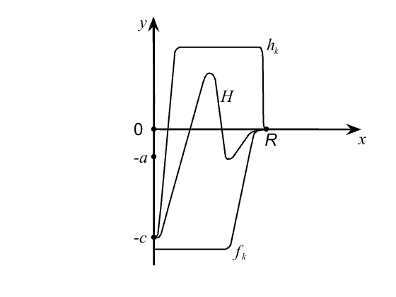
Refer to caption
Figure 3. The function HH

5.1. Proof of Theorem 1.6

Proof.

Let c=−supS1×MHc=-\sup_{S^{1}\times M}H. Then c>R​lαc>Rl_{\alpha}. Choose a∈[R​lα,c]a\in[Rl_{\alpha},c] so that a/R∉Λαa/R\notin\Lambda_{\alpha}. Then we can construct two sequences of functions {fk}k∈ℕ\{f_{k}\}_{k\in\mathbb{N}} and {hk}k∈ℕ\{h_{k}\}_{k\in\mathbb{N}} as in Section 4.3. For sufficiently large kk it follows that

Hfk≤H≤HhkH^{f_{k}}\leq H\leq H^{h_{k}}

as illustrated in Figure 3. Fix such an integer k=k⁡(H)k=k(H). Then by Proposition 4.2 we have the commutative diagram (4.3).

So the monotone homomorphism Ψhk​fk\Psi_{h_{k}f_{k}} is nonzero due to our assumption that μk≥a/R≥lα\mu_{k}\geq a/R\geq l_{\alpha}; see Remark 4.1. Applying Theorem 3.6 to the Hamiltonians HfkH^{f_{k}} and HhkH^{h_{k}}, there exist positive constants δ1=δ1​(Hfk,g,σ,a,α)\delta_{1}=\delta_{1}(H^{f_{k}},g,\sigma,a,\alpha) and δ2=δ2​(Hhk,g,σ,a,α)\delta_{2}=\delta_{2}(H^{h_{k}},g,\sigma,a,\alpha) such that if |δ|<δ0:=min⁡{δ1,δ2}|\delta|<\delta_{0}:=\min\{\delta_{1},\delta_{2}\}, then we have the following commutative diagram

HFα(a,+∞)​(Hfk)→Ψhk​fkHFα(a,+∞)​(Hhk)Ψω0ωδ​σ↓↓Ψω0ωδ​σHFα(a,+∞)​(Hfk,δ​σ)→Ψhk​fkδ​σHFα(a,+∞)​(Hhk,δ​σ)\displaystyle\begin{CD}{\rm HF}^{(a,+\infty)}_{\alpha}(H^{f_{k}})@>{\Psi_{h_{k}f_{k}}}>{}>{\rm HF}^{(a,+\infty)}_{\alpha}(H^{h_{k}})\\ @V{\Psi_{\omega_{0}}^{\omega_{\delta\sigma}}}V{}V@V{}V{\Psi_{\omega_{0}}^{\omega_{\delta\sigma}}}V\\ {\rm HF}^{(a,+\infty)}_{\alpha}(H^{f_{k}},\delta\sigma)@>{\Psi^{\delta\sigma}_{h_{k}f_{k}}}>{}>{\rm HF}^{(a,+\infty)}_{\alpha}(H^{h_{k}},\delta\sigma)\end{CD} (5.1)

Combining (4.3) and (5.1) we deduce that for |δ|<δ0|\delta|<\delta_{0} the monotone homomorphism Ψhk​fkδ​σ\Psi^{\delta\sigma}_{h_{k}f_{k}} is also nonzero. Given δ∈(−δ0,δ0)\delta\in(-\delta_{0},\delta_{0}), choose a sequence of Hamiltonian functions Hi∈ℋH_{i}\in\mathscr{H} such that HiH_{i} satisfy the non-degeneracy condition (C) and converge to HH in C∞C^{\infty} topology, Hfk≤Hi≤HhkH^{f_{k}}\leq H_{i}\leq H^{h_{k}}, a∉𝒮α​(Hi,δ​σ)a\notin\mathscr{S}_{\alpha}(H_{i},\delta\sigma) and supS1×MHi<−R​lα\sup_{S^{1}\times M}H_{i}<-Rl_{\alpha}. Then, by Lemma 2.3, the non-trivial homomorphism Ψhk​fkδ​σ\Psi^{\delta\sigma}_{h_{k}f_{k}} factors through the Floer homology group HFα(a,+∞)​(Hi,δ​σ){\rm HF}^{(a,+\infty)}_{\alpha}(H_{i},\delta\sigma). Hence there exists a sequence of periodic orbits xi∈𝒫α​(Hi,δ​σ)x_{i}\in\mathscr{P}_{\alpha}(H_{i},\delta\sigma) such that 𝒜Hi,δ​σ​(xi)>a\mathscr{A}_{H_{i},\delta\sigma}(x_{i})>a. Passing to a converging subsequence, we get a periodic orbit x∈𝒫α​(H,δ​σ)x\in\mathscr{P}_{\alpha}(H,\delta\sigma) with 𝒜H,δ​σ​(x)≥a\mathscr{A}_{H,\delta\sigma}(x)\geq a.

∎

5.2. Proof of Theorem 1.7

Proof.

Consider the Hamiltonian function defined by

H¯​(t,x):=−H⁡(−t,x)∀(t,x)∈S1×DR​T∗​M.\bar{H}(t,x):=-H(-t,x)\quad\forall\;(t,x)\in S^{1}\times D_{R}T^{*}M.

Let C⁡(α)=R​lαC(\alpha)=Rl_{\alpha}. Obviously, x⁡(t)x(t) is a periodic orbit of HH representing −α-\alpha if and only if x⁡(−t)x(-t) is a periodic orbit of H¯\bar{H} representing α\alpha, and it holds that

supS1×MH¯≤−C⁡(α).\sup_{S^{1}\times M}\bar{H}\leq-C(\alpha).

Imitating the proof of Theorem 1.6 with replacing Theorem 3.6 by Theorem 3.8 concludes the proof of Theorem 1.7.

∎

5.3. Proofs of Theorem 1.10 and Theorem 1.11

The idea of the proof of Theorem 1.10 is the same as that of Theorem 1.6, while the difference between the two proofs is that one can squeeze uniformly a class of functions (whose graphs lie in the grey region in Figure 4 and on the line y=0,x≥R−ρy=0,x\geq R-\rho) from above and below in the proof of Theorem 1.10. The proof of Theorem 1.11 is similar to that of Theorem 1.10. Here we only show the latter.

Refer to caption
Figure 4. A class of functions
Proof.

Let ϵ>0\epsilon>0 be an arbitrary number in (0,A−R​lα)(0,A-Rl_{\alpha}) and set c=R​lα+ϵc=Rl_{\alpha}+\epsilon. Pick a=a⁡(ϵ)∈[R​lα,c]a=a(\epsilon)\in[Rl_{\alpha},c] so that a/R∉Λαa/R\notin\Lambda_{\alpha}. Construct two sequences of functions {fk}k∈ℕ\{f_{k}\}_{k\in\mathbb{N}} and {hk}k∈ℕ\{h_{k}\}_{k\in\mathbb{N}} as in Section 4.3. Then there exists an integer k0=k0​(g,σ,α,V,A,ρ,ϵ)>0k_{0}=k_{0}(g,\sigma,\alpha,V,A,\rho,\epsilon)>0 such that

Hfk0≤H≤Hhk0H^{f_{k_{0}}}\leq H\leq H^{h_{k_{0}}}

for every H∈ℋc​(UR,UR−ρ,V,A)H\in\mathscr{H}_{c}(U_{R},U_{R-\rho},V,A). Following the proof of Theorem 1.6 shows that there exists a constant

δ0:=δ0​(g,σ,α,V,A,ρ,ϵ)>0\delta_{0}:=\delta_{0}(g,\sigma,\alpha,V,A,\rho,\epsilon)>0

such that if |δ|<δ0|\delta|<\delta_{0} then every H∈ℋc​(UR,UR−ρ,V,A)H\in\mathscr{H}_{c}(U_{R},U_{R-\rho},V,A) admits a 11-periodic Hamiltonian orbit with respect to the twisted symplectic form ωδ​σ\omega_{\delta\sigma} whose projection to MM represents α\alpha. Therefore, by definition, for each δ∈(−δ0,δ0)\delta\in(-\delta_{0},\delta_{0}) we have c^BPS​(UR,UR−ρ,V,A,δ​σ,α)≤R​lα+ϵ\hat{c}_{\rm BPS}(U_{R},U_{R-\rho},V,A;\delta\sigma,\alpha)\leq Rl_{\alpha}+\epsilon.

∎

5.4. Proofs of Theorem 1.15 and Theorem 1.16

The key to the proofs of Theorem 1.15 and Theorem 1.16 is the following monotonicity of the restricted BPS capacity.

Proposition 5.1.

Let W1,W2W_{1},W_{2} be open subsets of T∗​MT^{*}M containing MM, V2⊂V1⊂U1⊂U2V_{2}\subset V_{1}\subset U_{1}\subset U_{2}, W1⊂W2W_{1}\subset W_{2} and 0<A1≤A20<A_{1}\leq A_{2}, where Wi,Ui,ViW_{i},U_{i},V_{i}, i=1,2i=1,2 are open subsets of T∗​MT^{*}M and UiU_{i} have compact closure U¯i⊂Wi\bar{U}_{i}\subset W_{i}. Then it holds that

c^BPS​(W1,U1,V1,A1,σ,α)≤c^BPS​(W2,U2,V2,A2,σ,α).\hat{c}_{\rm BPS}(W_{1},U_{1},V_{1},A_{1};\sigma,\alpha)\leq\hat{c}_{\rm BPS}(W_{2},U_{2},V_{2},A_{2};\sigma,\alpha).

Our proof of Theorem 1.15 is an adaption of the standard almost existence theorem (see [31, Section 4.2] or [44]). For the sake of completeness we shall give a proof of Theorem 1.15. The proof of Theorem 1.16 is nearly identical to that of Theorem 1.15, we omit it here.

Proof.

Along the lines of [31, Section 4.2], we proceed in 3 steps.

Step 1. By our assumption, the sublevel {H<s}\{H<s\} is contained in Ur⁡(s)U_{r(s)}, where r:ℝ→(0,∞)r:\mathbb{R}\to(0,\infty) is a nondecreasing function. Consider the monotone functions c^δ:[d,T]→[0,∞]\hat{c}_{\delta}:[d,T]\to[0,\infty] defined by

c^δ(s):=c^BPS(Ur⁡(T+ρ)+ρ,{H<s},V,A;δσ,α).\hat{c}_{\delta}(s):=\hat{c}_{\rm BPS}(U_{r(T+\rho)+\rho},\{H<s\},V,A;\delta\sigma,\alpha).

Theorem 1.10 implies that there exists a constant δ0:=δ0​(g,σ,α,V,A,T,ρ)>0\delta_{0}:=\delta_{0}(g,\sigma,\alpha,V,A,T,\rho)>0 such that if |δ|<δ0|\delta|<\delta_{0} then

c^BPS​(Ur⁡(T+ρ)+ρ,Ur⁡(T+ρ),V,A,δ​σ,α)<A\hat{c}_{\rm BPS}(U_{r(T+\rho)+\rho},U_{r(T+\rho)},V,A;\delta\sigma,\alpha)<A

provided A>(r⁡(T+ρ)+ρ)​lαA>(r(T+\rho)+\rho)l_{\alpha}. Then we deduce from Proposition 5.1 that

c^δ​(s)≤c^δ​(T+ρ)≤c^BPS​(Ur⁡(T+ρ)+ρ,Ur⁡(T+ρ),V,A,δ​σ,α)<A∀s∈[d,T+ρ],\hat{c}_{\delta}(s)\leq\hat{c}_{\delta}(T+\rho)\leq\hat{c}_{\rm BPS}(U_{r(T+\rho)+\rho},U_{r(T+\rho)},V,A;\delta\sigma,\alpha)<A\quad\forall s\in[d,T+\rho],

where |δ|<δ0​(g,σ,α,V,A,T,ρ)|\delta|<\delta_{0}(g,\sigma,\alpha,V,A,T,\rho). Fix δ∈(−δ0,δ0)\delta\in(-\delta_{0},\delta_{0}). So Lebesgue’s last theorem implies that the function c^δ\hat{c}_{\delta} is differentiable at almost every point in the sense of measure theory. Suppose that s0∈[d,T]s_{0}\in[d,T] is a regular value of HH and c^δ\hat{c}_{\delta} is Lipschitz continuous at s0s_{0}. Then, by the implicit function theorem, S0:=H−1​(s0)S_{0}:=H^{-1}(s_{0}) is a hypersurface in T∗​MT^{*}M, which is compact and bounds the sublevel set B0:={H<s0}B_{0}:=\{H<s_{0}\} since HH is proper and bounded below. By the implicit function theorem again and compactness of S0S_{0}, one can find a parameterized family of hypersurfaces SεS_{\varepsilon} in T∗​MT^{*}M with Sε=H−1​(s0+ε)S_{\varepsilon}=H^{-1}(s_{0}+\varepsilon) such that

c⁡(ε)≤c⁡(0)+L​ε,c⁡(ε):=c^δ​(s0+ε)c(\varepsilon)\leq c(0)+L\varepsilon,\quad c(\varepsilon):=\hat{c}_{\delta}(s_{0}+\varepsilon)

for 0≤ε≤η0\leq\varepsilon\leq\eta, where LL and η\eta are positive constants. By choosing η\eta smaller, let us require that η<min⁡{ρ,(A−c⁡(0))/(2​L)}\eta<\min\{\rho,(A-c(0))/(2L)\} (A>c⁡(0)A>c(0) by our assumption). For 0<ε≤η0<\varepsilon\leq\eta, let us denote Bε:={H<s0+ε}B_{\varepsilon}:=\{H<s_{0}+\varepsilon\}, then Bε⊂{H<T+ρ}⊂Ur⁡(T+ρ)B_{\varepsilon}\subset\{H<T+\rho\}\subset U_{r(T+\rho)}. Fixing ς∈(0,η]\varsigma\in(0,\eta], we define a smooth function f:ℝ→[−2​L​ς,0]f:\mathbb{R}\to[-2L\varsigma,0] by

f⁡(s)=−2​L​ςif​s≤0f⁡(s)=0if​s≥ς20<f′​(s)≤8​Lif​ 0<s<ς2.\begin{array}[]{ll}f(s)=-2L\varsigma&\hbox{if}\;s\leq 0\\ f(s)=0&\hbox{if}\;s\geq\frac{\varsigma}{2}\\ 0<f^{\prime}(s)\leq 8L&\hbox{if}\;0<s<\frac{\varsigma}{2}.\end{array}

By the definition of the restricted BPS capacity c^δ​(s0)=c⁡(0)\hat{c}_{\delta}(s_{0})=c(0), there exists a Hamiltonian function G∈ℋ⁡(Ur⁡(T+ρ)+ρ,B0,A)G\in\mathscr{H}(U_{r(T+\rho)+\rho},B_{0},A) such that

−c⁡(0)<supVG≤−(c⁡(0)−L​ς)and𝒫α​(G,δ​σ,τ)=∅∀ 0<τ≤1.-c(0)<\sup_{V}G\leq-(c(0)-L\varsigma)\quad\hbox{and}\quad\mathscr{P}_{\alpha}(G,\delta\sigma;\tau)=\emptyset\quad\forall\;0<\tau\leq 1. (5.2)

Otherwise, c⁡(0)=c^δ​(s0)≤c⁡(0)−L​ςc(0)=\hat{c}_{\delta}(s_{0})\leq c(0)-L\varsigma which contradicts with the fact that L​ς≥0L\varsigma\geq 0. Now we constructed a new function G~\widetilde{G} by cutting off GG without creating new fast periodic orbits. More precisely, let χ:[−c⁡(0)−ϵ,−c⁡(0)+ϵ]→ℝ\chi:[-c(0)-\epsilon,-c(0)+\epsilon]\to\mathbb{R} be a function with 0≤χ′≤10\leq\chi^{\prime}\leq 1 such that χ⁡(t)=−c⁡(0)\chi(t)=-c(0) for tt near the left endpoint of the interval and χ⁡(t)=t\chi(t)=t for tt near the right endpoint of the interval, where ϵ>0\epsilon>0 is sufficiently small so that −c⁡(0)+ϵ<supVG-c(0)+\epsilon<\sup_{V}G. Set

G~​(x):={−c⁡(0)if​G​(x)≤−c⁡(0)−ϵ,χ⁡(G⁡(x))if−c⁡(0)−ϵ≤G⁡(x)≤−c⁡(0)+ϵ,G⁡(x)if−c⁡(0)+ϵ≤G⁡(x).\widetilde{G}(x):=\left\{\begin{array}[]{ll}-c(0)&\hbox{if}\;G(x)\leq-c(0)-\epsilon,\\ \chi(G(x))&\hbox{if}\;-c(0)-\epsilon\leq G(x)\leq-c(0)+\epsilon,\\ G(x)&\hbox{if}\;-c(0)+\epsilon\leq G(x).\end{array}\right.

The new non-positive function G~\widetilde{G} compactly supported in B0B_{0} satisfies

𝒫α​(G~,δ​σ,τ)=∅∀ 0<τ≤1\mathscr{P}_{\alpha}(\widetilde{G},\delta\sigma;\tau)=\emptyset\quad\forall\;0<\tau\leq 1

since |χ′|≤1|\chi^{\prime}|\leq 1. Furthermore, supVG~≤−(c⁡(0)−L​ς)\sup_{V}\widetilde{G}\leq-(c(0)-L\varsigma) and infB0G~≥−c⁡(0)\inf_{B_{0}}\widetilde{G}\geq-c(0). Consider the compactly supported Hamiltonian function K∈C∞​(Bς)K\in C^{\infty}(B_{\varsigma}) defined by

K​(x)=G~​(x)−2​L​ςif​x∈B0K⁡(x)=f⁡(ε)if​x∈Sε, 0≤ε<ςK⁡(x)=0if​x∉Bς.\begin{array}[]{ll}K(x)=\widetilde{G}(x)-2L\varsigma&\hbox{if}\;x\in B_{0}\\ K(x)=f(\varepsilon)&\hbox{if}\;x\in S_{\varepsilon},\;0\leq\varepsilon<\varsigma\\ K(x)=0&\hbox{if}\;x\notin B_{\varsigma}.\end{array}

The function KK satisfies

supVK=supVG~−2​L​ς≤−(c⁡(0)−L​ς)−2​L​ς≤−c⁡(ς)and\sup_{V}K=\sup_{V}\widetilde{G}-2L\varsigma\leq-(c(0)-L\varsigma)-2L\varsigma\leq-c(\varsigma)\quad\hbox{and}
infBςK=infB0G~−2​L​ς>−c⁡(0)−2​L​η>−A.\inf_{B_{\varsigma}}K=\inf_{B_{0}}\widetilde{G}-2L\varsigma>-c(0)-2L\eta>-A.

The definition of the restricted BPS capacity c⁡(ς)c(\varsigma) shows that KK has a fast periodic orbit xx with respect to ωδ​σ\omega_{\delta\sigma} whose projection to MM represents α\alpha. We claim that xx cannot intersect B0B_{0}. Indeed, if xx intersects B0B_{0} then it stays completely inside B0B_{0} since B0B_{0} is invariant under the flow of KK. This is impossible because the flows of KK and G~\widetilde{G} on B0B_{0} coincide and G~\widetilde{G} does not have fast periodic orbits. Since α≠0\alpha\neq 0, the fast periodic orbit xx whose projection represents α\alpha is nontrivial. As a consequence, xx must be contained in Bς∖B0¯B_{\varsigma}\setminus\overline{B_{0}}, and hence it lies on SεS_{\varepsilon} for some 0<ε<ς0<\varepsilon<\varsigma.

Step 2. Step 1 works for every ς∈(0,η]\varsigma\in(0,\eta]. Choosing a sequence ςj→0\varsigma_{j}\to 0, one can find sequences KjK_{j} and εj\varepsilon_{j}, and a corresponding sequence xj​(t)x_{j}(t) of periodic orbits of XKj,δ​σX_{K_{j},\delta\sigma} having periods 0<τj≤10<\tau_{j}\leq 1 and lying on SεjS_{\varepsilon_{j}} with εj→0\varepsilon_{j}\to 0. Consider the Hamiltonian HH on the set

U=⋃ε∈(−η,η)Sε.U=\bigcup\limits_{\varepsilon\in(-\eta,\eta)}S_{\varepsilon}.

Obviously, if x∈Sεx\in S_{\varepsilon} then H⁡(x)=s0+εH(x)=s_{0}+\varepsilon and Kj​(x)=fj​(ε)=fj​(H⁡(x)−s0)K_{j}(x)=f_{j}(\varepsilon)=f_{j}(H(x)-s_{0}). By construction, the periodic orbits xjx_{j} solve the equations

x˙j​(t)=fj′​(εj)​XH,δ​σ​(xj​(t))xj​(0)=x⁡(τj)\begin{array}[]{ll}\dot{x}_{j}(t)=f^{\prime}_{j}(\varepsilon_{j})X_{H,\delta\sigma}\big(x_{j}(t)\big)\\ x_{j}(0)=x(\tau_{j})\end{array}

with the periods 0≤τj≤10\leq\tau_{j}\leq 1. Normalizing the periods to 11 we define the functions

yj​(t)=xj​(τj​t)∀t∈[0,1]y_{j}(t)=x_{j}\big(\tau_{j}t\big)\quad\forall t\in[0,1]

which solve the Hamiltonian equations

y˙j​(t)=fj′​(εj)​τj​XH,δ​σ​(yj​(t))andH⁡(yj​(t))=εj.\dot{y}_{j}(t)=f^{\prime}_{j}(\varepsilon_{j})\tau_{j}X_{H,\delta\sigma}(y_{j}(t))\quad\hbox{and}\quad H\big(y_{j}(t)\big)=\varepsilon_{j}.

Step 3. By construction, fj′≤8​Lf^{\prime}_{j}\leq 8L and hence fj′​(εj)​τjf^{\prime}_{j}(\varepsilon_{j})\tau_{j} are bounded. This observation is very useful for us to obtain a periodic orbit on S0S_{0}. Indeed, we first note that the hypersurfaces SεjS_{\varepsilon_{j}} are contained in the compact set Bη¯\overline{B_{\eta}}, hence the functions xjx_{j} are uniformly bounded. For all t∈S1t\in S^{1} and all j∈ℕj\in\mathbb{N} we estimate

‖y˙j​(t)‖Gg=|fj′​(εj)​τj|⋅‖XH,δ​σ​(xj​(t))‖Gg≤8​L​supx∈Bη¯‖XH,δ​σ‖Gg.\|\dot{y}_{j}(t)\|_{G_{g}}=|f^{\prime}_{j}(\varepsilon_{j})\tau_{j}|\cdot\|X_{H,\delta\sigma}\big(x_{j}(t)\big)\|_{G_{g}}\leq 8L\sup_{x\in\overline{B_{\eta}}}\|X_{H,\delta\sigma}\|_{G_{g}}.

Then, by Arzela-Ascoli theorem, passing to subsequences, fj′​(εj)​τjf^{\prime}_{j}(\varepsilon_{j})\tau_{j} converges to some τ≥0\tau\geq 0 and yj​(t)y_{j}(t) converges in C0C^{0}-topology, and, by making use of the equations, even converges in C∞C^{\infty}-topology to a smooth 11-periodic solution yy of the equation

y˙​(t)=τ​XH,δ​σ​(y⁡(t)),y⁡(t)⊂S0.\dot{y}(t)=\tau X_{H,\delta\sigma}(y(t)),\quad y(t)\subset S_{0}.

We claim that τ≠0\tau\neq 0. Otherwise, y⁡(t)=y∗y(t)=y^{*} for some point y∗∈S0y^{*}\in S_{0}. This contradicts with the fact that the projection of yy on MM represents the non-trivial class α\alpha since [π⁡(yj)]=α[\pi(y_{j})]=\alpha and π⁡(yj)\pi(y_{j}) converges to π⁡(y)\pi(y) in C∞C^{\infty}-topology. Reparametrizing time we obtain the τ\tau-periodic solution x⁡(t):=y⁡(t/τ)x(t):=y(t/\tau) of the equation

x˙​(t)=XH,δ​σ​(x⁡(t))\dot{x}(t)=X_{H,\delta\sigma}(x(t))

whose projection on MM represents α\alpha. The proof of Theorem 1.15 is completed. ∎

5.5. Concluding remarks

5.5.1. Hamiltonian flows without non-contractible closed trajectories

The following proposition shows that the constant δ0​(H,g,σ,a,b,α)\delta_{0}(H,g,\sigma,a,b,\alpha) in Theorem 1.6 depends on HH. As a consequence, one can not extend Theorem 1.6 (resp. Theorem 1.7) to the case that δ0​(H,g,σ,a,b,α)\delta_{0}(H,g,\sigma,a,b,\alpha) (resp. δ0​(H,g,a,b,α)\delta_{0}(H,g,a,b,\alpha)) is arbitrarily large.

Proposition 5.2.

Let MM be a closed Riemanian surface endowed with a metric gg of constant curvature K=−1K=-1. Then there exists a sequence of compactly supported Hamiltonians {Hn}n∈ℕ⊂C∞​(D1​T∗​M)\{H_{n}\}_{n\in\mathbb{N}}\subset C^{\infty}(D_{1}T^{*}M) with infMHn>n\inf_{M}H_{n}>n and a sequence of numbers {δn}n∈ℕ\{\delta_{n}\}_{n\in\mathbb{N}} converging to 00 such that the periodic orbits of the Hamiltonian flow of HnH_{n} with respect to ωn=ω0+δn​π∗​σ\omega_{n}=\omega_{0}+\delta_{n}\pi^{*}\sigma are all contractible.

This proposition is due to Niche [40]. For the sake of completeness, we outline a proof of Proposition 5.2 below. The following proof is different from Niche’s proof and is based on a theorem of Ginzburg [21].

Proof.

We start with ω=ω0+π∗​d​A\omega=\omega_{0}+\pi^{*}dA where d​AdA is the area form on (M,g)(M,g). Further, let FF be the standard kinetic energy Hamiltonian. Then [21, Theorem 2.5] shows that on every level {F=c}\{F=c\} with c<1/2c<1/2 all integral curves of FF are closed and contractible, and there is no closed orbit on {F=1/2}\{F=1/2\} (on which the Hamiltonian flow is the horocycle flow, cf. [30]). Let V={F<1/2}V=\{F<1/2\}. Let χ:[0,1/2]→[0,C]\chi:[0,1/2]\to[0,C] be a “one-sided bump” function with χ′≤0\chi^{\prime}\leq 0 such that χ⁡(t)=C\chi(t)=C near t=0t=0 and χ⁡(t)=0\chi(t)=0 near t=1/2t=1/2. Here CC is a constant and can be made arbitrarily large. Let H=χ∘FH=\chi\circ F. Then HH is supported in VV. Moreover, the flow of HH is essentially a reparametrization of the flow of HH on VV and hence all orbits are closed and contractible.

Let us now replace the area form d​AdA by a new magnetic field δ​d​A\delta dA where 0<δ≤10<\delta\leq 1. The region VV will shrink to VδV_{\delta} or in other words the threshold level {F=1/2}\{F=1/2\} will get closer to MM getting replaced by {F=δ2/2}\{F=\delta^{2}/2\}. But everything else remains the same. Indeed, by a rescaling argument, the existence of closed trajectories of ω=ω0+δ​π∗​d​A\omega=\omega_{0}+\delta\pi^{*}dA on the energy level {F=δ2/2}\{F=\delta^{2}/2\} is equivalent to the existence of closed trajectories of ω=δ​ω0+δ​π∗​d​A\omega=\delta\omega_{0}+\delta\pi^{*}dA on the energy level {F=1/2}\{F=1/2\}. The flow of the later is a reparametrization of the flow of FF with respect to ω=ω0+π∗​d​A\omega=\omega_{0}+\pi^{*}dA on {F=1/2}\{F=1/2\}, and hence has no non-contractible periodic obits.

Finally, by taking some sequence {δn}n=1∞\{\delta_{n}\}_{n=1}^{\infty} satisfying δn→0\delta_{n}\to 0 and a sequence of Hamiltonians HnH_{n} obtained by composing the same FF with more and more narrow bump functions, we obtain the desired result.

∎

5.5.2. Counterexample

The condition {H<d}⊃M\{H<d\}\supset M in Theorem 1.15 and Theorem 1.16 cannot be dropped. The following example is given by Salomão and Weber [44].

Example 5.3.

Let M=S1=ℝ/ℤM=S^{1}=\mathbb{R}/\mathbb{Z}. Consider the function H:T∗​M=S1×ℝ→ℝH:T^{*}M=S^{1}\times\mathbb{R}\to\mathbb{R} given by

H⁡(q,p)=12​‖p‖g2+V⁡(q),H(q,p)=\frac{1}{2}\|p\|_{g}^{2}+V(q),

where V⁡(q)=1+c​o​s​2​π​qV(q)=1+cos2\pi q. Then {H<1}\{H<1\} does not contain MM, and for any energy s∈[1,2)s\in[1,2) the level set H=s{H=s} does not carry non-contractible periodic orbits.

6. Appendix. The proof of Proposition 4.2

To prove Proposition 4.2, we need a theorem of Weber in [51] that computes Floer homology of convex radial Hamiltonians.

Theorem 6.1 ([51, Theorem 2.9]).

Let f:ℝ→ℝf:\mathbb{R}\to\mathbb{R} be a smooth symmetric function with f′′≥0f^{\prime\prime}\geq 0. If τ∈ℝ+∖Λα\tau\in\mathbb{R}^{+}\setminus\Lambda_{\alpha} and f′​(r)=τf^{\prime}(r)=\tau for some r>0r>0, then there is a natural isomorphism

Φfτ:HFα(−∞,bf,τ)​(Hf)→H∗​(ℒατ2/2​M),bf,τ:=r​f′​(r)−f⁡(r).\Phi_{f}^{\tau}:{\rm HF}^{(-\infty,b_{f,\tau})}_{\alpha}(H^{f})\to{\rm H}_{*}(\mathcal{L}_{\alpha}^{\tau^{2}/2}M),\quad b_{f,\tau}:=rf^{\prime}(r)-f(r). (6.1)

If HhH^{h} is another such Hamiltonian, then there exists an isomorphism Ψh​fτ\Psi_{hf}^{\tau} such that the following diagram commutes:

HFα(−∞,bf,τ)​(Hf)\textstyle{{\rm HF}^{(-\infty,b_{f,\tau})}_{\alpha}(H^{f})\ignorespaces\ignorespaces\ignorespaces\ignorespaces\ignorespaces\ignorespaces\ignorespaces\ignorespaces}≃\scriptstyle{\simeq}Ψh​fτ\scriptstyle{\Psi_{hf}^{\tau}}≃\scriptstyle{\simeq}Φfτ\scriptstyle{\Phi_{f}^{\tau}}HFα(−∞,bh,τ)​(Hh)\textstyle{{\rm HF}^{(-\infty,b_{h,\tau})}_{\alpha}(H^{h})\ignorespaces\ignorespaces\ignorespaces\ignorespaces}≃\scriptstyle{\simeq}Φhτ\scriptstyle{\Phi_{h}^{\tau}}H∗​(ℒατ2/2​M)\textstyle{{\rm H}_{*}(\mathcal{L}_{\alpha}^{\tau^{2}/2}M)}

If ρ∈(0,τ]∖Λα\rho\in(0,\tau]\setminus\Lambda_{\alpha} and f′​(s)=ρf^{\prime}(s)=\rho for some s>0s>0, then we have the following communicative diagram whose top horizonal row is the natural inclusion ιF\iota^{F}:

HFα(−∞,bf,ρ)​(Hf)→ιFHFα(−∞,bf,τ)​(Hf)Φfρ↓≃≃↓ΦfτH∗​(ℒαρ2/2​M)→[ιτ2/2​ρ2/2]H∗​(ℒατ2/2​M)\displaystyle\begin{CD}{\rm HF}^{(-\infty,b_{f,\rho})}_{\alpha}(H^{f})@>{\iota^{F}}>{}>{\rm HF}^{(-\infty,b_{f,\tau})}_{\alpha}(H^{f})\\ @V{\Phi_{f}^{\rho}}V{\simeq}V@V{\simeq}V{\Phi_{f}^{\tau}}V\\ {\rm H}_{*}(\mathcal{L}_{\alpha}^{\rho^{2}/2}M)@>{{[\iota^{\tau^{2}/2}{\rho^{2}/2}}]}>{}>{\rm H}_{*}(\mathcal{L}_{\alpha}^{\tau^{2}/2}M)\end{CD} (6.7)

Here the Floer homology HFα(a,b)​(Hf){\rm HF}^{(a,b)}_{\alpha}(H^{f}) is well defined for every Hf∈𝒦R;αa,bH^{f}\in\mathscr{K}_{R;\alpha}^{a,b}; see Remark 2.5.

Refer to caption
Figure 5. The monotone homotopy between fkf_{k} and fk′f_{k}^{\prime}
Proof of Proposition 4.2.

The basic idea is to deform fkf_{k} and hkh_{k} by monotone homotopies to convex functions so that Theorem 6.1 can be applied. To show the isomorphism (4.1), first, we follow the graph of fkf_{k} until the slope of it becomes aa for the second time at a point, saying pp, near rk​2r_{k2}, then continue linearly with slope aa, we obtain a function which is of C1C^{1}-class at pp. Then smoothing out such a function near pp yields a smooth function fk′∈𝒦R;α−∞,af_{k}^{\prime}\in\mathscr{K}_{R;\alpha}^{-\infty,a} (see Figure 5). The monotone homotopy between fkf_{k} and fk′f_{k}^{\prime}, as showed in Figure 5, provides the monotone isomorphism

Ψfk′​fk:HFα(a,+∞)​(Hfk)→HFα(a,+∞)​(Hfk′).\Psi_{f_{k}^{\prime}f_{k}}:{\rm HF}^{(a,+\infty)}_{\alpha}(H^{f_{k}})\to{\rm HF}^{(a,+\infty)}_{\alpha}(H^{f^{\prime}_{k}}). (6.8)

This is the consequence of the fact that the yy-intercepts of the tangential line at all points that do not remain constant during the homotopy are strictly larger than −a-a.

Refer to caption
Figure 6. The monotone homotopy between fk′f_{k}^{\prime} and fk′′f_{k}^{\prime\prime}

Second, we define the function fk′′f_{k}^{\prime\prime} obtained by following the the graph fk′f_{k}^{\prime} until the slope of it becomes aa for the first time at some point qq; then continue linearly with slope aa (see Figure 6). The result function is of C1C^{1}-class at qq. Smoothing near qq we obtain a smooth function fk′′∈𝒦R;α−∞,af_{k}^{\prime\prime}\in\mathscr{K}_{R;\alpha}^{-\infty,a}. Note that all tangential lines of the graphs during the monotone homotopy, as indicated in Figure 6, which pass through the point (0,−a)(0,-a) lie strictly between the lines x↦a​x/R−ax\mapsto ax/R-a and x↦l0​x−ax\mapsto l_{0}x-a. It follows that the homotopy between fk′f_{k}^{\prime} and fk′′f_{k}^{\prime\prime} induces the monotone isomorphism

Ψfk′′​fk′:HFα(a,+∞)​(Hfk′)→HFα(a,+∞)​(Hfk′′).\Psi_{f_{k}^{\prime\prime}f_{k}^{\prime}}:{\rm HF}^{(a,+\infty)}_{\alpha}(H^{f^{\prime}_{k}})\to{\rm HF}^{(a,+\infty)}_{\alpha}(H^{f_{k}^{\prime\prime}}). (6.9)

Since the yy-intercept of the tangential line of graph fk′′f_{k}^{\prime\prime} at any point is less than −a-a, the action of 𝒜Hfk′′\mathscr{A}_{H^{f_{k}^{\prime\prime}}} at each 11-periodic orbit is larger than aa. Then the exact sequence (2.9) yields isomorphisms

HFα(a,+∞)​(Hfk′′)→HFα(−∞,+∞)​(Hfk′′)→HFα(−∞,B)​(Hfk′′).{\rm HF}^{(a,+\infty)}_{\alpha}(H^{f_{k}^{\prime\prime}})\xrightarrow{}{\rm HF}^{(-\infty,+\infty)}_{\alpha}(H^{f_{k}^{\prime\prime}})\to{\rm HF}^{(-\infty,B)}_{\alpha}(H^{f_{k}^{\prime\prime}}). (6.10)

Here B=bfk′′,a/RB=b_{f_{k}^{\prime\prime},a/R} is defined in Theorem 6.1 (the fact that a/R∉Λαa/R\notin\Lambda_{\alpha} is used). Then by Theorem 6.1 we have the natural isomorphism

Φfk′′a/R:HFα(−∞,B)​(Hfk′′)→H∗​(ℒαa2/(2​R2)​M).\Phi_{f_{k}^{\prime\prime}}^{a/R}:{\rm HF}^{(-\infty,B)}_{\alpha}(H^{f_{k}^{\prime\prime}})\to{\rm H}_{*}(\mathcal{L}_{\alpha}^{a^{2}/(2R^{2})}M). (6.11)

By composing (6.8)-(6.11) we arrive at the desired isomorphism (4.1).

Refer to caption
(a) The monotone homotopy between hkh_{k} and hk′h_{k}^{\prime}
Refer to caption
(b) The monotone homotopy between hk′h_{k}^{\prime} and hk′′h_{k}^{\prime\prime}
Figure 7. Monotone homotopies

To obtain the isomorphism (4.2), we deform hkh_{k} initially by the monotone homotopy as showed in Figure 7 (a) to a smooth function hk′h_{k}^{\prime}, then keep on deforming hk′h_{k}^{\prime} by the monotone homotopy (see Figure 7 (b)) to a smooth function hk′′h_{k}^{\prime\prime}. Here if x≥R+εx\geq R+\varepsilon for some sufficiently small positive constant ε\varepsilon, the graph of hk′′h_{k}^{\prime\prime} turns into a ray with slope μk\mu_{k} which is very close to the line x→μk​x−ax\to\mu_{k}x-a. Note that all points on members of the homotopy whose tangential lines pass through the point (0,−a)(0,-a) lie strictly between the lines l−​x−al_{-}x-a and l+−al_{+}-a ; see Figure 7. Therefore we obtain the monotone isomorphisms

HFα(a,+∞)​(Hhk)→Ψhk′​hkHFα(a,+∞)​(Hhk′)→Ψhk′′​hk′HFα(a,+∞)​(Hhk′′).{\rm HF}^{(a,+\infty)}_{\alpha}(H^{h_{k}})\xrightarrow{\Psi_{h_{k}^{\prime}h_{k}}}{\rm HF}^{(a,+\infty)}_{\alpha}(H^{h^{\prime}_{k}})\xrightarrow{\Psi_{h_{k}^{\prime\prime}h_{k}^{\prime}}}{\rm HF}^{(a,+\infty)}_{\alpha}(H^{h^{\prime\prime}_{k}}). (6.12)
Refer to caption
Figure 8. The monotone homotopy between hk′′h_{k}^{\prime\prime} and h~k\tilde{h}_{k}

Next, consider function h~k\tilde{h}_{k} given by following the graph of hk′′h_{k}^{\prime\prime} until it takes on slope μk\mu_{k} for the first time (near the point (0,−c)(0,-c)); then continue linearly with slope μk\mu_{k} (see Figure 8). Smoothing near (0,−c)(0,-c) yields h~k\tilde{h}_{k}. Since the yy-intercepts of the tangential lines of the graphs during the homotopy as showed in 8 are less than −a-a, we obtain the monotone isomorphism

Ψh~k​hk′′:HFα(a,+∞)​(Hhk′′)→HFα(a,+∞)​(Hh~k).\Psi_{\tilde{h}_{k}h_{k}^{\prime\prime}}:{\rm HF}^{(a,+\infty)}_{\alpha}(H^{h_{k}^{\prime\prime}})\to{\rm HF}^{(a,+\infty)}_{\alpha}(H^{\tilde{h}_{k}}). (6.13)

Again, using the fact that the yy-intercepts of the tangential lines of the graph h~k\tilde{h}_{k} are less than −a-a, the exact sequence (2.9) implies the following isomorphisms:

HFα(a,+∞)​(Hh~k)→HFα(−∞,+∞)​(Hh~k)→HFα(−∞,B′)​(Hh~k){\rm HF}^{(a,+\infty)}_{\alpha}(H^{\tilde{h}_{k}})\to{\rm HF}^{(-\infty,+\infty)}_{\alpha}(H^{\tilde{h}_{k}})\to{\rm HF}^{(-\infty,B^{\prime})}_{\alpha}(H^{\tilde{h}_{k}}) (6.14)

where B′=bh~k,μkB^{\prime}=b_{\tilde{h}_{k},\mu_{k}} is as in (6.1). Then Theorem 6.1 gives the isomorphsim

Φh~kμk:HFα(−∞,B′)​(Hh~k)→H∗​(ℒαμk2/2​M).\Phi_{\tilde{h}_{k}}^{\mu_{k}}:{\rm HF}^{(-\infty,B^{\prime})}_{\alpha}(H^{\tilde{h}_{k}})\to{\rm H}_{*}(\mathcal{L}_{\alpha}^{\mu_{k}^{2}/2}M). (6.15)

Composing  (6.12) - (6.15) yields the desired isomorphism (4.2).

The proof of (4.3) is identical to that of the communicative diagram (53) in [51] without any essential changes; see p.563 and p. 564, which is an easy application of Theorem 6.1, we omit it here. ∎

References

  • [1] A. Abbondandolo, L. Macarini, M. Mazzucchelli and G. P. Paternain, Infinitely many periodic orbits of exact magnetic flows on surfaces for almost every subcritical energy level, J. Eur. Math. Soc. 19 (2017), 551-579.
  • [2] L. Asselle and G. Benedetti, The Lusternik-Fet theorem for autonomous Tonelli Hamiltonian systems on twisted cotangent bundles. J. Topol. Anal. 8 (2016), 545-570.
  • [3] M. Audin and J. Lafontaine (Eds), Holomorphic curves in symplectic geometry, Progress in Mathematics, Birkhäuser Verlag, Basel, 117 (1994).
  • [4] Y. Bae and U. Frauenfelder, Continuation homomorphism in Rabinowitz Floer homology for symplectic deformations, Math. Proc. Cambridge Philos. Soc. 151 (2011), 471-502.
  • [5] M. Batoréo, On non-contractible periodic orbits of symplectomorphisms. J. Symplectic Geom. 15 (2017), 687-717.
  • [6] G. Benedetti and A. F. Ritter. Invariance of symplectic cohomology and twisted cotangent bundles over surfaces. Preprint (2018), available at http://arxiv.org/abs/1807.02086, (2018).
  • [7] P. Biran, L. Polterovich and D. Salamon, Propagation in Hamiltonian dynamics and relative symplectic homology, Duke Math. J. 119 (2003), 65-118.
  • [8] K. Cieliebak, Symplectic boundaries: Creating and destroying closed characteristics. Geom. Funct. Anal. 7 (1997), 269-321.
  • [9] K. Cieliebak, A. Floer and H. Hofer, Symplectic homology, II. A general construction, Math. Z. 218 (1995), 103-122.
  • [10] K. Cieliebak, V. L. Ginzburg and E. Kerman, Symplectic homology and periodic orbits near symplectic submanifolds. Comment. Math. Helv. 79 (2004), 554-581.
  • [11] A. Floer, Morse theory for Lagrangian intersections. J. Differential Geom. 28 (1988), 513-547.
  • [12] A. Floer, The unregularized gradient flow of the symplectic action. Comm. Pure Appl. Math. 41 (1988), 775-813.
  • [13] A. Floer, Witten’s complex and infinite-dimensional Morse theory. J. Differential Geom. 30 (1989), 207-221.
  • [14] A. Floer and H. Hofer, Symplectic homology, I. Open sets in ℂn\mathbb{C}^{n}, Math. Z. 215 (1994), 37-88.
  • [15] A. Floer, H. Hofer and D. Salamon, Transversality in elliptic Morse theory for the symplectic action. Duke Math. J. 80 (1995), 251-292.
  • [16] U. Frauenfelder, W. Merry and P. Paternain, Floer homology for magnetic fields with at most linear growth on the universal cover. J. Funct. Anal. 262 (2012), 3062-3090.
  • [17] U. Frauenfelder, W. Merry and P. Paternain, Floer homology for non-resonant magnetic fields on flat tori. Nonlinearity 28 (2015), 1351-1370.
  • [18] U. Frauenfelder and F. Schlenk, Hamiltonian dynamics on convex symplectic manifolds. Israel J. Math. 159 (2007), 1-56.
  • [19] D. Gatien and F. Lalonde, Holomorphic cylinders with Lagrangian boundaries and Hamiltonian dynamics, Duke Math. J. 102 (2000), 485-511.
  • [20] V. L. Ginzburg, On closed trajectories of a charge in a magnetic field. An application of symplectic geometry, in Contact and symplectic geometry Vol. 8 (Publication of 5 the Newton Institute, Cambridge University Press, 1996), pp. 131-148.
  • [21] V. L. Ginzburg, On the existence and non-existence of closed trajectories for some Hamiltonian flows. Math. Z. 223 (1996), 397-409.
  • [22] V. L. Ginzburg and B. Z. Gürel, Relative Hofer-Zehnder capacity and periodic orbits in twisted cotangent bundles. Duke Math. J. 123 (2004), 1-47.
  • [23] V. L. Ginzburg and B. Z. Gürel, Periodic orbits of twisted geodesic flows and the Weinstein-Moser theorem. Comment. Math. Helv. 84 (2009), 865-907.
  • [24] V. L. Ginzburg and B. Z. Gürel, Non-contractible periodic orbits in Hamiltonian dynamics on closed symplectic manifolds. Compos. Math. 152 (2016), 1777-1799.
  • [25] V. L. Ginzburg and E. Kerman. Periodic orbits in magnetic fields in dimensions greater than two. In Geometry and topology in dynamics (Winston-Salem, NC, 1998/San Antonio, TX, 1999). Contemp. Math, 246. Amer. Math. Soc., Providence, 1999, 113-121.
  • [26] W. Gong, Symplectic deformations of Floer homology and non-contractible periodic orbits in twisted disc bundles. Preprint (2018), available at http://arxiv.org/abs/1801. 08773, (2018).
  • [27] Y. Groman and W. J. Merry, The symplectic cohomology of magnetic cotangent bundles. Preprint (2018), available at http://arxiv.org/abs/1809. 01085, (2018).
  • [28] M. Gromov, Asymptotic invariants of infinite groups. Geometric group theory II, G.A. Niblo and M.A. Roller, London Math. Soc. Lecture Notes 182 (1993), pp. 1-295.
  • [29] B. Z. Gürel, On non-contractible periodic orbits of Hamiltonian diffeomorphisms. Bull. Lond. Math. Soc. 45 (2013), 1227-1234.
  • [30] G. A. Hedlund, Fuchsian groups and transitive horocycles. Duke Math. J. 2 (1936), 530-542.
  • [31] H. Hofer and E. Zehnder, Symplectic Invariants and Hamiltonian Dynamics, Birkhauser Advanced Texts, Birkhauser, (1994).
  • [32] K. Irie, Hofer-Zehnder capacity of unit disk cotangent bundles and the loop product. J. Eur. Math. Soc. 16 (2014), 2477-2497.
  • [33] M. Kawasaki and R. Orita, Computation of annular capacity by Hamiltonian Floer theory of non-contractible periodic trajectories. J. Mod. Dyn. 11 (2017), 313-339.
  • [34] G. Lu, The Weinstein conjecture on some symplectic manifolds containing the holomorphic spheres, Kyushu J. Math. 52 (1998), 331-351.
  • [35] G. Lu, The Conley conjecture for Hamiltonian systems on the cotangent bundle and its analogue for Lagrangian systems. J. Funct. Anal. 256 (2009), 2967-3034.
  • [36] G. Lu, Corrigendum to ”The Conley conjecture for Hamiltonian systems on the contangent bundle and its analogue for Lagrangian systems” [J. Funct. Anal. 256 (9) (2009) 2967-3034]. J. Funct. Anal. 261 (2011), 542-589.
  • [37] G. Lu, Finiteness of the Hofer-Zehnder capacity of neighborhoods of symplectic submanifolds, Int. Math. Res. Not. (2006), Art. ID 76520, 33 pp.
  • [38] W. J. Merry, Closed orbits of a charge in a weakly exact magnetic field. Pacific J. Math. 247 (2010), 189-212.
  • [39] W. J. Merry, On the Rabinowitz Floer homology of twisted cotangent bundles. Calc. Var. Partial Differential Equations 42 (2011), 355-404.
  • [40] C. J. Niche, Non-contractible periodic orbits of Hamiltonian flows on twisted cotangent bundles, Discrete Contin. Dyn. Syst. 14 (2006), 617-630.
  • [41] L. Polterovich, Growth of maps, distortion in groups and symplectic geometry, Invent. Math. 150 (2002), 655-686.
  • [42] M. Poźniak, “Floer homology, Novikov rings, and clean intersections” In Northern California Symplectic Geometry Seminar, Amer. Math. Soc. Transl., Ser. 2, 196, AMS, Providence, 1999, 119-181.
  • [43] A. F. Ritter, Deformations of symplectic cohomology and exact Lagrangians in ALE spaces. Geom. Funct. Anal. 20 (2010), 779-816.
  • [44] P. A. S. Salomão and J. Weber, An almost existence theorem for non-contractible periodic orbits in cotangent bundles. São Paulo J. Math. Sci. 6 (2012), 385-394.
  • [45] D. Salamon, Lectures on Floer homology, in: Y. Eliashberg, L. Traynor (Eds.), Symplectic Geometry and Topology, in: IAS/Park City Math. Ser., vol. 7, Amer. Math. Soc., 1999, pp. 143-225.
  • [46] D. Salamon and E. Zehnder, Morse theory for periodic solutions of Hamiltonian systems and the Maslov index. Comm. Pure Appl. Math. 45 (1992), 1303-1360.
  • [47] P. Seidel, Graded Lagrangian submanifolds. Bull. Soc. Math. France 128 (2000), 103-149.
  • [48] J. C. Sikorav, Growth of a primitive of a differential form. Bull. Soc. Math. France 129 (2001), 159-168.
  • [49] M. Usher, Floer homology in disk bundles and symplectically twisted geodesic flows. J. Mod. Dyn. 3 (2009), 61-101.
  • [50] C. Viterbo, Functors and computations in Floer homology with applications, I, Geom. Funct. Anal. 9 (1999), 985-1033.
  • [51] J. Weber, Noncontractible periodic orbits in cotangent bundles and Floer homology, Duke Math. J. 133 (2006), 527-568.
  • [52] J. Weber, Perturbed closed geodesics are periodic orbits: index and transversality. Math. Z. 241 (2002), 45-82.
  • [53] J. Xue, Existence of noncontractible periodic orbits of Hamiltonian systems separating two Lagrangian tori on T∗​𝕋nT^{*}\mathbb{T}^{n} with application to nonconvex systems. J. Symplectic Geom. 15 (2017), 905-936.
  • [54] J. Zhang, Symplectic structure perturbations and continuity of symplectic invariants. Preprint (2016), available at http://arxiv.org/abs/1610.00516, (2016).