From Neuronal Models to Neuronal Dynamics and Image Processing
1 Introduction
Neurons make contacts with each other by synapses: The presynaptic neuron sends its output to the synapse via an axon, and
the postsynaptic neuron receives it via its dendritic tree (“dendrite”). Most neurons produce their output in form of
virtually binary events (action potentials or spikes). Some classes of neurons (e.g., in the retina) nevertheless do not
generate spikes but show continuous responses.
Dendrites were classically considered as passive cables whose only function is to transmit input signals to the soma ( cell
body of the neuron). In this picture, a neuron integrates all input signals and generates a response if their sum exceeds
a threshold. Therefore, the neuron is the site where computations take place, and information is stored across the network in
synaptic weights (“connection strengths”). This “connectionist” point of view on neuronal functioning inspired neuronal
networks learning algorithms such as error backpropagation [1], and more recent deep-learning architectures
[2]. Recent evidence, however, suggest that dendrites are excitable structures rather than passive
cables, which can perform sophisticated computations [3, 4, 5, 6].
This suggest that even single neurons can carry out far more complex computations than previously thought.
Naturally, a modeller has to choose a reasonable level of abstraction. A good model is not necessarily one which incorporates all possible
details, because too many details can make it difficult to identify important mechanisms. The level of detail is related to the research
question that we wish to answer, but also to our computational resources [7]. For example, if our interest was to
understanding the neurophysiological details of a small circuit of neurons, then we probably would choose a Hodgkin-Huxley model
for each neuron [8] and also include detailed models of dendrites, axons, and synaptic dynamic and learning.
A disadvantage of the Hodgkin-Huxely model is its high computational complexity. It requires about floating point operations
(FLOPS) for the simulation of ms of time [9].
Therefore, if we want to simulate a large network with many neurons, then we may omit dendrites, axons and use a simpler model
such as the integrate-and-fire neuron model (which is presented further down) or the Izhikevich model [10].
The Izhikevich model offers the same rich spiking dynamics as the full Hodgkin-Huxley model (e.g. bursting, tonic spiking, …), while
having a computational complexity similar to the integrate-and-fire neuron model (about and FLOPSms, respectively).
Further simplifications can be made if we aim at simulating psychophysical data, or at solving image processing tasks. For example,
spiking mechanisms are often not necessary then, and we can compute a continuous response (as opposed to binary spikes)
from the neuron’s state variable (e.g., membrane potential) by thresholding (half-wave rectification, e.g. ) or via
a sigmoidal function (“squashing function”, e.g. ).
This chapter approaches neural modeling and computational neuroscience, respectively, in a tutorial-like fashion. This
means that basic concepts are explained by way of simple examples, rather than providing an in-depth review on a specific
topic. We proceed by first introducing a simple neuron model (the membrane potential equation), which is derived by
considering a neuron as an electrical circuit. When the membrane potential equation is augmented with a spiking mechanism,
it is known as the leaky integrate-and-fire model. “Leaky” means that the model forgets exponentially fast about past inputs.
“Integrate” means that it sums its inputs, which can be excitatory (driving the neuron towards its response threshold) or
inhibitory (drawing the state variable away from the response threshold). Finally, “fire” refers to the spiking mechanism.
The membrane potential equation is subsequently applied to three image processing tasks. Section 3 presents a
reaction-diffusion-based model of the retina, which accounts for simple visual illusions and afterimages.
Section 4 describes a model for segregating texture features that is inspired by computations
in the primary visual cortex [11]. Finally, section 5 introduces a model of a
collision-sensitive neuron in the locust visual system [12]. The last section discusses
a few examples where image processing (or computer vision) methods also could explain how the brain processes
the corresponding information.
2 The Membrane Equation as a Neuron Model
In order to derive a simple yet powerful neuron model, imagine the neuron’s cell membrane (comprising dendrites, soma, and axon)
as a small sphere. The membrane is a bilayer of lipids, which is -Å thick (Åmnm).
It isolates the extracellular space from a cell’s interior, and thus forms a barrier for different ion species, such as (sodium), (potassium),
and (chloride).
Now if the ionic concentrations in the extracellular fluid and the cytoplasm ( cell’s interior) were all the same, then one would be probably
dead. Neuronal signalling relies on the presence of ionic gradients. With all cells at rest (i.e., neither input nor output), about half of the
brain’s energy budget is consumed for moving to the outside of the cell and inward (the - -pump).
Some types of neurons also pump outside (via the -transporter). The pumping mechanisms compensate for the ions
that leak through the cell membrane in the respective reverse directions, driven by electrochemical gradients. At rest, the neuron
therefore maintains a dynamic equilibrium.
We are now ready to model the neuron as an electrical circuit, where a capacitance (cell membrane) is connected in parallel with a (serially
connected) resistance and a battery. The battery sets the cell’s resting potential . In particular, all (neuron-, glia-, muscle-)
cells have a negative resting potential, typically mV. The resting potential is the value of the membrane voltage
when all ionic concentrations are in their dynamic equilibrium. This is of course a simplification since we lump together the diffusion
potentials (such as or ) of each ion species. The simplification comes at a cost, however,
and our resulting neuron model will not be able to produce action potentials or spikes by itself (the binary events by which many
neurons communicate with each other) without explicitly adding a spike-generating mechanism (more on that in section 2.2).
By Ohm’s law, the current that leaks through the membrane is , where the leakage
conductance is just the inverse of the membrane resistance.
The charge which is kept apart by a cell’s membrane with capacitance is . Whenever the neuron signals, the
distribution of charges changes, and so does the membrane potential, and thus will be non-zero.
In other words, a current will flow, carried by ions. Assuming some fixed value for , the change in will be slower
for a higher capacitance (better buffering capacity). Kirchhoff’s current law is the equivalent of current conservation
, or
| (1) |
The right hand side corresponds to current flows due to excitation and inhibition (more on that later). Biologically, current flows occur
across protein molecules that are embedded in the cell membrane. The various protein types implement specific functions such as ionic
channels, enzymes, pumps, and receptors.
These “gates” or “doors” through the cell membrane are highly specific, such that only particular information or substances (like ions)
can enter or exit the cell. Strictly speaking, each channel which is embedded in a neuron’s cell membrane would corresponds to a RC-circuit
( resistance, capacitance) such as equation 1. But fortunately, neurons are very small, what
justifies the assumption that channels are uniformly distributed, and the potential does not vary across the cell membrane: The cell is said
to be isopotential, and it can be adequately described by a single RC-compartment.
Let’s assume that we have nothing better to do than waiting for a sufficiently long time such that the neuron reaches equilibrium.
Then, by definition, is constant, and thus . What remains from the last equation is just , or
. In the absence of excitation and inhibition we have and the neuron will be at its resting potential.
But how long do we have to wait until the equilibrium is reached? To find that out, we just move all terms with to one side
of the equation, and the term which contains time to the other. This technique is known as separation of variables, and
permits integration in order to convert the infinitesimal quantities and into ”normal” variables (we formally rename
the corresponding integration variables for time and voltage as and , respectively),
| (2) |
where . We furthermore define . Integration of the left hand side gives . With the (membrane) time constant of the cell , the above equation yields
| (3) |
It is easy to see that for we get , where in the absence of external
currents (this confirms our previous result). The time that we have to wait until this equilibrium is reached depends on :
The higher the resistance , and the bigger the capacitance , the longer it will take (and vice versa).
The constant has to be selected according to the initial conditions of the problem. For example, if we assume that the
neuron is at rest when we start the simulation, then , and therefore
| (4) |
2.1 Synaptic Inputs
Neurons are not loners but are massively connected to other neurons. The connection sites are called synapses. Synapses come in two
flavours: Electrical and chemical. Electrical synapses (also called gap junctions) can directly couple the membrane potential of neighbouring neurons.
In this way, distinct networks of specific neurons are formed, usually between neurons of the same type. Examples of electrically coupled neurons
are retinal horizontal cells [13, 14], cortical low-threshold-spiking interneurons, and cortical fast-spiking interneurons
[15, 16] (interneurons are inhibitory). Sometimes chemical and electrical synapses even combine to permit reliable and
fast signal transmission, such as it is the case in the locust, where the Lobula Giant Movement Detector (LGMD) connects to the Descending
Contralateral Movement Detector (DMCD) [17, 18, 19, 20].
Chemical synapses are far more common than gap junctions. In one cubic millimeter of cortical grey matter there are about one billion ()
chemical synapses (ca. in the whole human brain). Synapses are usually plastic. Whether they increase or decrease their connection
strength to a post-synaptic neuron depends on causality. If a pre-synaptic neuron fires within some ms before the post-synaptic neuron,
the connection gets stronger (potentiation: ”P”) [21]. In contrast, if the pre-synaptic spike arrives
after activation of the post-synaptic neuron, synaptic strength is decreased (depression: ”D”) [22]. This mechanism is known as
spike time dependent plasticity (STDP), and can be identified with Hebbian learning [23, 24].
Synaptic potentiation is thought to be triggered by back-propagating calcium spikes in the dendrites of post-synaptic neuron [25]
Synaptic plasticity can occur over several timescales, short term (ST) and long term (LT). Remember these acronyms if you see letter
combinations like “LTD”, “LTP”, “STP” or “STD”.
An activation of fast, chemical synapses causes a rapid and transient voltage change in the post-synaptic neuron. These voltage changes
are called post-synaptic potentials (PSPs). PSPs can be either inhibitory (IPSPs) or excitatory (EPSPs). Excitatory neurons
depolarize their target neurons ( will get more positive as a consequence of the EPSP), whereas inhibitory neurons hyperpolarize
their post-synaptic targets. How can we model synapses? PSPs are caused by a temporary increase in membrane conductance in series
with a so-called synaptic reversal battery (also synaptic reversal potential, or synaptic battery). The synaptic input
defines the current on the right hand side of equation 1,
| (5) |
The last equation sums synaptic inputs, each with conductance and reversal potential . Notice that whether an input acts excitatory or inhibitory on the membrane potential depends usually on whether the synaptic battery is bigger or smaller than the resting potential . Just consider only one type of excitatory and inhibitory input. Then we can write
| (6) |
(For all simulations, if not otherwise stated, we assume and omit the physical units).
How to solve this equation? After converting the differential equation into a difference equation, the equation can be solved
numerically with standard integration schemes, such as Euler’s method, Runge-Kutta, Crank-Nicolson, or Adams-Bashforth (see
for example chapter 6 in [26] and chapter 17 in [27] for more details). Typically, model
neurons are integrated with a step size of ms or less, as this is the relevant time scale for neuronal signalling. If the
simulation focusses more on perceptual dynamics (or biologically-inspired image processing tasks), then one may choose a bigger
integration time constant as well. The ideal integration method is stable, produces solutions with a high accuracy, and has a
low computational complexity. In practice, of course, we have to make the one or the other trade-off.
Remember that is called leakage conductance, which is just the inverse of the membrane resistance.
For constant capacitance , the leakage conductance determines the time constant of the neuron:
Bigger values of will make it ”faster” (i.e. less memory on past inputs), while smaller values will cause a higher
degree of low-pass filtering of the input. and is the excitatory and inhibitory
synaptic battery, respectively.
For the synaptic current (mainly and ) is inward and negative by convention.
The membrane thus gets depolarized. This is a signature of an EPSP. In the brain, the most common type of excitatory
synapses release glutamate (a neurotransmitter)11
1
In the peripheral nervous system of vertebrates, excitatory
synapses are activated instead by acetylcholine (ACh). The neurotransmitter diffuses across the synaptic cleft, and
binds on glutamate-sensitive receptors in the post-synaptic cell membrane. As a consequence, ion channels will open,
and and (but also via voltage sensitive channels) will enter the cell.
Agonists are pharmacological substances that do not exist in the brain, but open these channels as well.
For instance, the agonist NMDA22
2
-methyl-D-aspartat will open excitatory, voltage-sensitive NMDA-channels.
AMPA33
3
-amino-3-hydroxy-5-methyl-4-isoxalone propionic acid is another agonist that
activates fast excitatory synapses. However, AMPA-synapses will remain silent in the presence of NMDA, and vice
versa. Therefore one can imagine the ionic channels as locked doors. For their opening, the right key is necessary,
which is either a specific neurotransmitter, or some “artificial” pharmacological agonist. The “locks” are the receptor sites
to which a neurotransmitter or an agonist binds. The reversal potentials of the fast AMPA-synapse is about mV
above the resting potential. Usually, AMPA-channels co-occur with NMDA-channels, what may enhance the computational
power of a neuron [28].
For the membrane is hyperpolarized. For , it gets less sensitive to depolarization,
and accelerates the return to for any synaptic input.
Pre-synaptic release of GABA44
4
From ref. [29]: -aminobutryc acid can activate three subtypes of receptors:
GABAA, GABAB, and GABAC (as before, they are identified through the action of specific pharmalogicals)55
5
GABAA,
are ligand-gated ion channels permeable to . Post-synaptic GABAB are heptahelical receptors coupled to inwardly rectifying
channels. Finally, GABAC are ligand-gated channels, which are primarily expressed in the retina.
Why are the synaptic batteries also called reversal potentials? For excitatory input, imposes an upper limit on .
This means that no matter how big will be, it can drive the neuron only up to . In order to understand that,
consider , the so-called driving potential: If , then the driving potential is high, and the
neuron depolarizes fast. The closer gets to , the smaller the driving potential, until the excitatory current
eventually approaches zero. (Analog considerations hold for the inhibitory input).
What is the value of at equilibrium? Equilibrium means that does not change with , and then the
left hand side of equation 6 is zero. Of course this implies that all excitatory and inhibitory
inputs vary sufficiently slow and we can consider them as being constant. Or, otherwise expressed, the neuron reaches
the equilibrium before a significant change in or takes place. Then, solving equation
6 for yields
| (7) |
The time until the equilibrium is reached depends not only on , but on all other active conductances.
As a consequence, a neuron which receives continuously input from other neurons can react faster than a
neuron which starts from [30]. (Ongoing cortical activity is the
normal situation, where it is thought that excitation and inhibition are just balanced [31]).
A specially interesting case is defined by , which is called silent or shunting inhibition.
It is silent because it only gets evident if the neuron is depolarized (and hyperpolarized if more than one type
of inhibition is considered). Shunting inhibition decreases the time constant of the neuron, thus making it faster.
In this way, the return to the resting potential
is accelerated, for excitatory and inhibitory input. Furthermore, divisive inhibition is a special form of
shunting inhibition if . With spiking neurons, however, pure divisive inhibition does not seem to
exist. In that case, shunting inhibition is rather subtractive [32] and cannot act as a gain control
mechanism. But in networks with balanced excitation and inhibition, the choice is ours’: If we change the
balance between excitation and inhibition, then the effect on a neuron’s response will be additive and subtractive,
respectively. If we leave the balance unchanged and increase or decrease excitation and inhibition in parallel,
then a multiplicative or divisive effect on a neuron’s response will occur [33].

2.2 Firing Spikes
Equation 6 represents the membrane potential of a neuron, but could represent different quantities as well.
For example, could be interpreted directly as response probability if we set, for example, , , and .
Accordingly, in the latter case we have . Another possibility is to set . As neuronal responses are only positive,
however, has to be half-wave rectified, meaning that we take as the output of the neuron66
6
In
this case, the response threshold . For arbitrary thresholds .. Naturally, half-wave rectification makes
only sense if negative values of can occur. Because of the absence of explicit spiking, the neuron’s output represents a (mean) firing rate,
usually interpreted as spikes per second.
When should one use equation 6 or 7? This depends
mainly on the purpose of the simulation. When the synaptic input consists of spikes, then one needs some
mechanism to convert them into continuous quantities. The low-pass filtering characteristics of equation
6 will do that. For instance, spikes are necessary for implementing spike-time-dependent
plasticity (STDP), which modifies synaptic strength dependent on pre- and postsynaptic activity.
For some purposes (e.g. biologically-inspired image processing), spikes are not strictly necessary, and one can use
the (mean or instantaneous) firing rate (or activity, that is the rectified membrane potential) of pre-synaptic
neurons directly as input to post-synaptic neurons. In that case, both equation 6
or 7 could be used. The steady-state solution (equation 7),
however, has less computational complexity, as one does not need to integrate it numerically. Recall that when using the steady-state
solution, one implicitly assumes that the synaptic input varies on a relatively slow time scale, such that the neuron can reach its
equilibrium state in each moment.
It is straightforward to convert 6 into a leaky integrate-and-fire neuron.
The term “leaky” refers to the leakage conductance , and the neuron would only be a perfect integrator for
As soon as the membrane potential crosses the neuron’s response threshold , we record a pulse with some
amplitude in the neuron’s response. Otherwise the response is usually defined as being zero:
In order to account for afterhyperpolarization (i.e., the refractory period), is set to some value after each spike. Usually, is chosen. The refractory period of a neuron is the time that the ionic pumps need to re-establish the original ion charge distributions. Within the absolute refractory period, the neuron will not spike at all, or spiking probability will be greatly reduced (relative refractory period). Other spiking mechanisms are conceivable as well. For example, we can define the model neuron’s response as being identical to firing rate , and add a spike to whenever . Then would represent a spiking threshold:
The response thus switches between a rate code () and a spike code () [34, 35].
A typical spike train produced by the latter mechanism is shown in figure 1b.
How are binary events such as spikes converted into post-synaptic potentials (PSPs)? A PSP has a sharp rise and a smooth decay,
and therefore is usually broader than the spike by which it was evoked. Assume that a spike arrives at time at the
post-synaptic neuron. Then the time course of the corresponding PSP (i.e. the excitatory or inhibitory input to the neuron)
is adequately described by the so-called -function:
| (8) |
The constant is chosen such that matches the desired maximum of the PSP.
The Heaviside function is is zero for , and otherwise. It makes sure
that the PSP generated by the spike at starts at time . The total synaptic input
into the neuron is , multiplied with a synaptic weight .
Instead of using the -function, we can simplify matters (and accelerate our simulation) by assuming that each spike
causes an instantaneous increase in or , respectively, followed by an exponential decay. Doing so
just amounts to adding one simple differential equation to our model neuron:
| (9) |
The time constant determines the rate of the exponential decay (faster decay if smaller), is the synaptic weight, and is the Kronecker Delta function, which is just one if its argument is zero: The -th spike increments by . The last equation low-pass filters the spikes. An easy-to-compute discrete version can be obtained by converting the last equation into a finite difference equation, either by forward or backward differencing (details can be found in section S8 of ref. [36]):
| (10) |
For forward differentiation, , where is the integration time constant that comes from approximating
by . For backward differencing, . The degree of low-pass filtering
( filter memory on past inputs) is determined by . For , the filter output just reproduces the input
spike pattern (the filter is said to have no memory on past inputs). For , the filter ignores any input spikes, and stays
forever at the value with which it was initialized (“infinite memory”). For any value between zero and one, filtering takes place,
where filtering gets stronger with increasing .
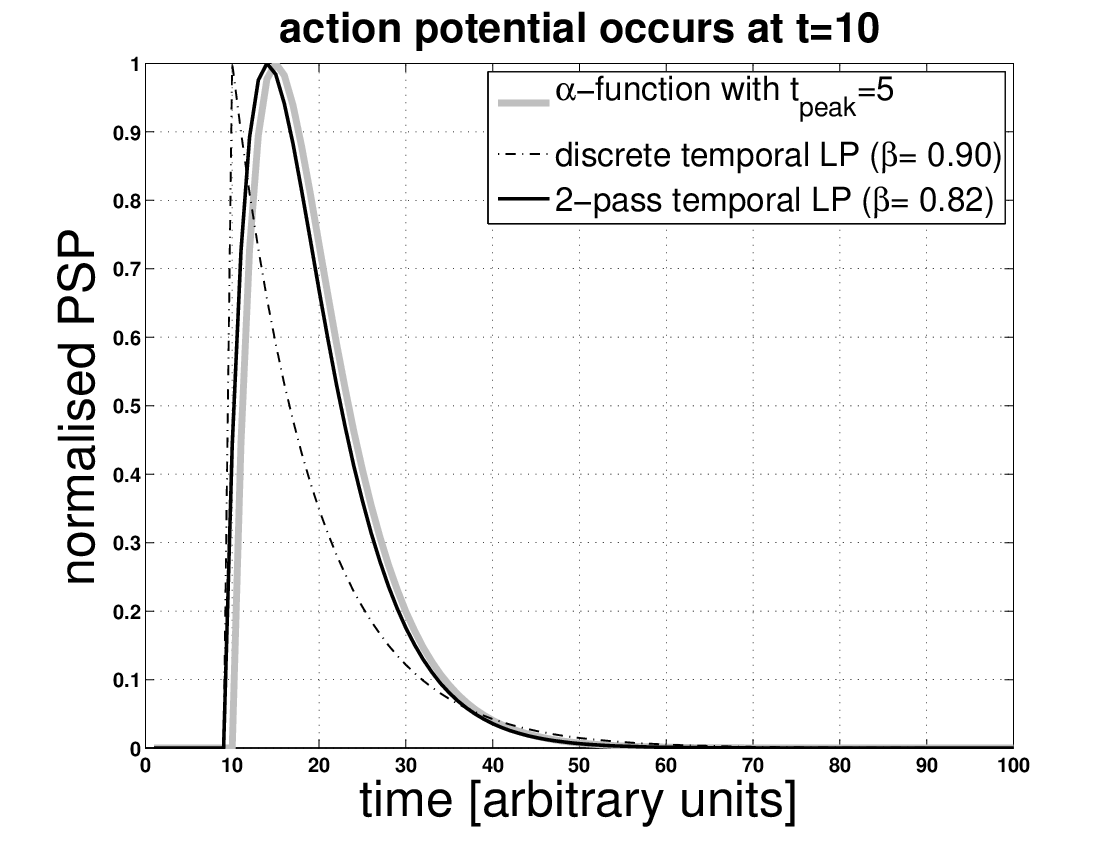
When one (or more) spikes are filtered by equation 10, then we see a sudden increase in at time , followed by
a gradual decay (figure 1a, dashed curve). This sudden increase stands in contrast to the gradual increase of the
PSP as predicted by equation 8 (figure 1a, gray curve). A better approximation to the shape of
a PSP results from applying low-pass filtering twice, as shown by the black curve in figure 1a. This is tantamount
to simulating two equations 10 for each synaptic input to equation 6.


3 Application 1: A dynamical retinal model
The retina is a powerful computational device. It transforms light intensities with different wavelengths – as being captures by cones (and rods for low-light vision) – into an efficient representation which is sent to the brain by the axons of the retinal ganglion cells [37]. The term “efficient” refers to redundancy reduction (“decorrelation”) in the stimulus on the one hand, and coding efficiency at the level of ganglion cells on the other. Decorrelation means that predictable intensity levels in time and space are suppressed in the responses of ganglion cells [38, 39]. For example, a digital photograph of a clear blue sky has a lot of spatial redundancy, because if we select a blue pixel, it is highly probable that its neighbours are blue pixels as well [40]. Coding efficiency is linked to metabolic energy consumption. Energy consumption increases faster than information transmission capacity, and organisms therefore seem to have evolved to a trade-off between increasing their evolutionary fitness and saving energy [41]. Retinal ganglion cells show efficient coding in the sense that noisy or energetically expensive coding symbols are less “used” [42, 37]. Often, the spatial aspects of visual information processing by the retina are grossly approximated by employing the Difference-of-Gaussian (“DoG”) model (one Gaussian is slightly broader than the other) [43]. The Gaussians are typically two-dimensional, isotropic, and centered at identical spatial coordinates. The resulting DoG model is a convolution kernel with positive values in the center surrounded by negative values. In mathematical terms, the DoG-kernel a filter that takes the second derivative of an image. In signal processing terms, it is a bandpass filter (or a highpass filter if a small kernel is used). In this way the center-surround antagonism of (foveal) retinal ganglion cells can be modelled [44]: ON-center ganglion cells respond when the center is more illuminated than the surround (i.e., positive values after convolving the DoG kernel with an image). OFF-cells respond when the surround receives more light intensity than the center (i.e., negative values after convolution). The DoG model thus assumes symmetric ON- and OFF-responses, what is again a simplification: Differences between biological ON- and OFF ganglion cells include receptive field size, response kinetics, nonlinearities, and light-dark adaptation [45, 46, 47]. Naturally, convolving an image with a DoG filter neither cannot account for adaptation nor dynamical aspects of retinal information processing. On the other hand, however, many retinal models which target the explanation of physiological or psychophysical data are not suitable for image processing tasks. So, biologically-inspired image processing means that the model should solve an image processing task (e.g., boundary extraction, dynamic range reduction), while at the same time produce predictions or has features which are by and large consistent with psychophysics and biology (e.g. brightness illusions, kernels mimicking receptive fields, etc.). In this spirit we now introduce a simple dynamical model for retinal processing, which re-produces some interesting brightness illusions an could even account for afterimages. An afterimage is an illusory percept where one continues to see a stimulus which is physically not present any more (e.g. a spot after looking into a bright light source). Unfortunately, the author was unable to find a version of the model which could be strictly based on equation 6. Instead of that, here is an even more simpler version that is based on the temporal low-pass filter (equation 10). Let be a gray level image with luminance values between zero (dark) and one (white). The number of iterations is denoted by ( discrete time). Then:
| (11) | |||||
| (12) |
where ON-cell responses, OFF-cell responses, is the diffusion coefficient,
is the diffusion operator (Laplacian), which was discretized as a
convolution kernel with in the center, and in north, east, south, and west pixels. Corner pixels were zero.
Thus, whereas the receptive field center is just one pixel, the surround is dynamically constructed by diffusion. Diffusion length (and
thus surround size) depends on the filter memory constant and the diffusion coefficient (bigger values will produce a
larger surround area).
Figure 2 shows four test images which were used for testing the dynamic retina model. The image 2a
shows a visual illusion (“grating induction”), where observers perceive an illusory modulation of luminance between the two gratings,
although luminance is actually constant. Figure 3a shows that the dynamic retina predicts a wave-like activity pattern
between the grating via . Because ON-responses represent brightness ( perceived luminance) and
OFF-responses represent darkness ( perceived inverse luminance) , the dynamic retina correctly predicts grating induction.
Does it also account for the absence of grating induction in figure 2b? The corresponding simulation is shown in
figure 3b, where the amplitude of the wave-like pattern is strongly reduced, and the frequency has doubled.
Thus, the absence of grating induction is adequately predicted.
In its equilibrium state, the dynamic retina performs contrast enhancement or boundary detection, respectively. This is illustrated with
the ON- and OFF-responses (figure 4a and 4b, respectively) to the image of figure 2c.
In comparison to an ordinary DoG-filter, however, the responses of the dynamic retina are asymmetric, with somewhat higher OFF-responses
to a luminance step (not shown). A nice feature of the dynamic retina is the prediction of after images. This is illustrated by
computing first the responses to a luminance staircase (figure 2d), and then replacing the staircase image by
the image of the camera man (figure 2c). Figure 4c,d shows corresponding responses immediately
after the images were swapped. Although the camera man image is now assigned to , a slightly blurred afterimage of the
staircase still appears in . The persistence of the afterimage depends on the luminance values: Higher intensities in
the first image, and lower intensities in the second image will promote a prolonged effect.


4 Application 2: Texture segregation
Networks based on equation 6 can be used for biologically plausible image processing tasks.
Nevertheless, the specific task that one wishes to achieve may imply modifications of equation 6.
As an example we outline a corresponding network for segregating texture from gray scale image (“texture system”).
We omit many mathematical details at this point (cf. chapter 4 in [11]), because they probably would make
reading too cumbersome.
The texture system forms part of a theory for explaining early visual information processing ([11]).
The essential proposal is that simple cells in V1 (primary visual cortex) segregate the visual input into texture, surfaces,
and (slowly varying) luminance gradients. This idea emerges quite naturally from considering how the symmetry and scale
of simple cells relate to features in the visual world: Simple cells with small and odd-symmetric receptive fields (RFs)
respond preferably to contours that are caused by changes in material properties of objects such as reflectance:
Object surfaces are delimited by odd-symmetric contours. Likewise, even-symmetrical simple cells respond
particularly well to lines and points, which we call texture in this context. Texture features are often superimposed on
object surfaces. Texture features may be variable and rather be irrelevant to recognize a certain object (e.g. if the object
is covered by grains of sand), but also may correspond to an identifying feature (e.g. tree bark).
Finally, simple cells at coarse resolutions (i.e, those with big RFs of both symmetries) are supposed to detect shallow
luminance gradients. Luminance gradients are a pictorial depth cue for resolving the three-dimensional
layout of a visual scene. However, they should be ignored for determining the material properties of object surfaces.
The first computational step in each of the three systems consists in detecting the respective features. Following feature
detection, representations of surfaces [48], gradients [49, 50, 51],
and texture [11], respectively, are eventually build by each corresponding system. Our normal visual
perception would then be the result of superimposing all three representations (brightness perception). Having
three separate representations (instead of merely a single one) has the advantage that higher-level cortical information
processing circuits could selectively suppress or reactivate texture and/or gradient representations in addition to surface
representations. This flexibility allows for the different requirements for deriving the material properties of objects.
For instance, surface representations are directly linked to the perception of reflectance (“lightness”) and object recognition,
respectively. In contrast, the computation of surface curvature and the interpretation of the three-dimensional scene structure
relies on gradients (e.g., shape from shading) and/or texture representations (texture compression with distance).
How do we identify texture features? We start with processing a gray scale image with a retinal model which is
based on a modification of equation 6:
| (13) |
is just the input image itself - so the center kernel (aka receptive field) is just one pixel.
is the result of convolving the input image with a surround kernel that has at
north, east, west and south position. Elsewhere it is zero. Thus, approximates
the (negative) second spatial derivative of the image. Accordingly we can define two types of ganglion cell
responses: ON-cells are defined by and respond preferably to (spatial) increments in luminance.
OFF-cells have and prefer decrements in luminance.
Figure 5b shows the output of equation 13, which is the half-wave rectified membrane potential
. Biological ganglion cell responses saturate with increasing contrast. This is modeled here
by , where corresponds to self-inhibition - the more center and surround are activated,
the stronger. Mathematically, , with a constant
that determines how fast the responses saturate. Why did we not simply set (and ), and
(and ) in equation 6 (vice versa for an OFF-cell)? Because in the
latter case ON and OFF response amplitudes would be different for a luminance step (cf. equation 7).
Luminance steps are odd-symmetric features and are not texture. Thus, we want to suppress them, and suppression is easier
if ON and OFF response amplitudes (to odd-symmetric features) are equal.
In response to even-symmetric features (i.e., texture features) we can distinguish two (quasi one-dimensional) response patterns.
A black line on a white background produces an ON-OFF-ON (LDL) response: A central OFF-response, and two flanking OFF-responses
with much smaller amplitudes. Analogously, a bright line on a dark background will trigger a OFF-ON-OFF or DLD response pattern.
ON- and OFF responses to lines (and edges) vary essentially in one dimension. Accordingly, we analyze them along
four orientations. Orientation selective responses (without blurring!) are established by convolving the OFF-channel
with an oriented Gaussian kernel, and subtract it from the (not blurred) ON-channel. This defines texture brightness.
The channel for texture darkness is defined by subtracting blurred ON responses from OFF responses. Subsequently,
even-symmetric response patterns are further enhanced with respect to surface features. In order to boost
a DLD pattern, the left-OFF is multiplied with its central-ON and its right-OFF (analogous for LDL patterns).
Note that surface response pattern (LD or DL, respectively) ideally has only one flanking response.
Dendritic trees are a plausible neurophysiological candidate for implementing such a “logic” AND gate
(simultaneous left and central and right response) [6].
In the subsequent stage the orientated texture responses are summed across orientations, leaving non-oriented responses
(Figure 5c).
By means of a winner-takes-all (WTA) competition between adjacent (non-oriented) texture brightness (“L”)
and texture darkness (“D”) it is now possible to suppress the residual surface features on the one hand, and the flanking
responses from the texture features on the other. For example, a LDL response pattern will generate a competition between
L and D (on the left side) and D and L (right side). Since for a texture feature the central response is bigger, it will
survive the competition with the flanking responses. The flanking responses, however, will not. A surface response
(say DL) will not survive either, because D- and L-responses have equal amplitudes. The local spatial WTA-competition is
established with a nonlinear diffusion paradigm [52]. The final output of the texture system (i.e., a
texture representation) is computed according to equation 6, where texture brightness acts excitatory,
and texture darkness inhibitory. An illustration of a texture representation is shown in figure 5d.


5 Application 3: Detection of collision threats
Many animals show avoidance reactions in response to rapidly approaching objects or other animals [53, 54].
Visual collision detection also has attracted attention from engineering because of its prospective applications, for example in robotics
or in driver assistant systems. It is widely accepted that visual collision detection in biology is mainly based on two angular variables:
(i) The angular size of an approaching object, and (ii) its angular velocity or rate of expansion
(the dot denotes derivative in time). If an object approaches an observer with constant velocity, then both angular
variables show a nearly exponential increase with time. Biological collision avoidance does not stop here, but computes mathematical
functions (here referred to as optical variables) of and . Accordingly, three principal
classes of collision-sensitive neurons have been identified [55]. These classes of neurons can be found in animals
as different as insects or birds. Therefore, evolution came up with similar computational principles that are shared across many
species [36].
A particularly well studied neuron is the Lobula Giant Movement Detector neuron (LGMD) of the locust visual system, because
the neuron is relatively big and easy to access. Responses of the LGMD to object approaches can be described by the so-called
eta-function: [56]. There is some evidence
that the LGMD biophysically implements [57] (but see [58, 59, 60]): Logarithmic encoding
converts the product into a sum, with representing excitation and inhibition. One distinctive
property of the eta-function is a response maximum before collision would occur. The time of the response maximum is determined
by the constant and always occurs at the fixed angular size .
So much for the theory - but how can the angular variables be computed from a sequence of image frames? The model which is
presented below (first proposed in [12]) does not compute them explicitly, although its output resembles the eta-function.
However, the eta-function is not explicitly computed either. Without going too far into an ongoing debate on the biophysical details of
the computations which are carried out by the LGMD [53, 61, 58], the model rests on lateral inhibition
in order to suppress self-motion and background movement [62].
The first stage of the model computes the difference between two consecutive image frames and (assuming gray scale videos):
| (14) |
where - we omit spatial indices and time for convenience. The last equation and all subsequent ones derives
directly from equation 6. Further processing in the model proceeds along two parallel pathways. The ON-pathway
is defined by the positive values of , that is . The OFF-pathway is defined by .
In the absence of background movement, is related to angular velocity: If an approaching object is yet far away,
then the sum will increase very slowly. In the last phase of an approach (shortly before collision), however, the sum increases steeply.
The second stage are two diffusion layers (one for ON, another one for OFF) that implement lateral inhibition:
| (15) |
where is the diffusion coefficient (cf. equation 12). The diffusion layers act inhibitory (see below) and serve to attenuate
background movement and translatory motion as caused by self-movement. If an approaching object is sufficiently far away, then the spatial
variations (as a function of time) in are small. Similarly, translatory motion at low speed will also generate small spatial displacements. Activity propagation proceeds at constant
speed and thus acts as a predictor for small movement patterns. But diffusion cannot keep up with those spatial variations as they are
generated in the late phase of an approach. The output of the diffusion layer is and ,
respectively (the tilde denotes half-wave rectified variables).
The input into the diffusion layers and , respectively,
is brought about by feeding back activity from the third stage of the model:
| (16) |
with excitatory input and inhibitory input
( and analogously). Hence, receives two types of inhibition from . First,
directly inhibits via the inhibitory input . Second, gates the excitatory input : Activity from the
first stage is attenuated at those positions where . This means that can only decrease where and feedback
from to assures that also the activity in will not grow further then. In this way it is largely avoided that the diffusion
layers continuously accumulate activity and will eventually “drown” (i.e., at all positions ). Drowning
otherwise would occur in the presence of strong background motion, making the model essentially blind to object approaches. The use
of two diffusion layers contributes to a further reduction of drowning.
The fifth and final stage of the model represents the LGMD neuron and spatially sums the output from the previous stage:
| (17) |
where and and analogously for . is a synaptic weight. Notice that whereas and are two-dimensional variables in space, is a scalar. The final model output corresponds to the two half-wave rectified LGMD activities and , respectively. Figure 6 shows representative frames from two video sequences that were used as input to the model. Figure 7 shows the corresponding output as computed by the last equation. Simulated LGMD responses are nice and clean in the absence of background movement (Figure 7a). The presence of background movement, on the other hand, produces spurious LGMD activation before collision occurs (Figure 7b).
6 Conclusions
Neurodynamical models (which are suitable for processing real-world images) and PDE (partial differential equation)-based image processing algorithms typically differ in the way they are designed, and in their respective predictions with regard to neuroscience. PDE-based image processing algorithms derive often from an optimization principle (such as minimizing an energy functional). As a result, a set of differential equations is usually obtained which evolves over time [63]. Many of these algorithms are designed ad hoc for specific image processing tasks (e.g. optical flow computation [64], segmentation [65], or denoising [66]), but they are usually not designed according to neuronal circuits. Similarly they usually do not predict psychophysical results. Some remarkable exceptions, however, do exist. For example, the color enhancement algorithm described in reference [67] is based on a perceptually motivated energy functional, which includes a contrast term (enforcing local contrast enhancement) and a dispersion term (implementing the gray-world assumption and enforcing fidelity to the data). In a similar vein could the Retinex algorithm - for estimating perceived reflectance (lightness) - also be casted into a variational framework [68]. An algorithm for tone mapping of high dynamic range images was originally motivated by compressing high contrasts while preserving low contrasts [69]. Although the authors did not explicitly acknowledge any inspiration from neuroscience, it is nevertheless striking how the algorithm resembles filling-in architectures [48]. Filling-in has been proposed as a mechanism for computing smooth representations of object surfaces in the visual system. Smooth representations means that surfaces are “tagged” with perceptual value such as color, movement direction, depth or lightness [70]. Filling-in is often modeled by (lateral) activity propagation within compartments, which are defined through contrast boundaries [71]. A recently proposed filling-in based computer vision algorithm identifies regions with a coherent movement direction from a (initially noisy) optic flow field [72]. The algorithm proposes also a solution to the so-called aperture problem, and is based on corresponding computations of the brain’s visual system [73]. A further method that resembles the filling-in process is image impainting (e.g., [74]). Image impainting completes missing regions by propagating the structure of the surround into that region. Although image impainting has not been related to neurophysiological principles, similar (slow) filling-in effects seem to exist also in the brain (e.g., texture filling-in [75]).
Acknowledgements
MSK acknowledges support from a Ramon & Cajal grant from the Spanish government, the “Retención de talento” program from the University of Barcelona, and the national grants DPI2010-21513 and PSI2013-41568-P.
References
- [1] Rumelhart, D. E., Hinton, G. E. and Williams, R. J., “Learning representations by back-propagating errors,” Nature, 323, p. 533–536, 1986.
- [2] Hinton, G. E. and Salakhutdinov, R. R., “Reducing the dimensionality of data with neural networks,” Science, 313, pp. 504–507, 2006.
- [3] Mel, B., “Information processing in dendritic trees,” Neural Computation, 6, pp. 1031–1085, 1994.
- [4] Häusser, M., Spruston, N. and Stuart, G., “Diversity and dynamics of dendritic signalling,” Science, 290, pp. 739–744, 2000.
- [5] Segev, I. and London, M., “Untangling dendrites with quantitative models,” Science, 290, pp. 744–750, 2000.
- [6] London, M. and Häusser, M., “Dendritic computation,” Annual Review of Neuroscience, 28, pp. 503–532, 2005.
- [7] Brette, R. et al., “Simulation of networks of spiking neurons: a review of tools and strategies,” Journal of Computational Neuroscience, 23, pp. 349–398, 2007.
- [8] Hodkin, A. and Huxley, A., “A quantitative description of membrane current and its application to conduction and excitation in nerve,” Journal of Physiology, 117, pp. 500–544, 1952.
- [9] Izhikevich, E., “Which model to use for cortical spiking neurons?” IEEE Transactions on Neural Networks, 15, pp. 1063–1070, 2004.
- [10] Izhikevich, E., “Simple model of spiking neurons,” IEEE Transactions on Neural Networks, 14, pp. 1569–1572, 2003.
- [11] Keil, M., Neural Architectures for Unifying Brightness Perception and Image Processing, Ph.D. thesis, Universität Ulm, Faculty for Computer Science, Ulm, Germany, 2003, http://vts.uni-ulm.de/doc.asp?id=3042.
- [12] Keil, M., Roca-Morena, E. and Rodríguez-Vázquez, A., “A neural model of the locust visual system for detection of object approaches with real-world scenes,” in “Proceedings of the Fourth IASTED International Conference,” volume 5119, pp. 340–345, Marbella, Spain, 2004, https://arxiv.org/abs/1801.08108.
- [13] Kolb, H., “The organization of the outer plexiform layer in the retina of the cat: Electron microscopic observations,” Journal of Neurocytology, 6, pp. 131–153, 1977.
- [14] Nelson, R. et al., “Spectral mechanisms in cat horizontal cells,” in “Neurocircuitry of the Retina: A Cajal Memorial,” pp. 109–121, Elsevier, New York, 1985.
- [15] Galarreta, M. and Hestrin, S., “A network of fast-spiking cells in the neocortex connected by electrical synapses,” Nature, 402, pp. 72–75, 1999.
- [16] Gibson, J., Beierlein, M. and Connors, B., “Two networks of electrically coupled inhibitory neurons in neocortex,” Nature, 402, pp. 75–79, 1999.
- [17] O’Shea, M. and Rowell, C., “A spike-transmitting electrical synapse between visual interneurones in the locust movement detector system,” Journal of Comparative Physiology, 97, pp. 875–885, 1975.
- [18] Rind, F., “A chemical synapse between two motion detecting neurones in the locust brain,” Journal of Experimental Biology, 110, pp. 143–167, 1984.
- [19] Killmann, F. and Schürmann, F., “Both electrical and chemical transmission between the lobula giant movement detector and the descending contralateral movement detector neurons of locusts are supported by electron microscopy,” Journal of Neurocytology, 14, pp. 637–652, 1985.
- [20] Killmann, F., Gras, H. and Schürmann, F., “Types, numbers and distribution of synapses on the dendritic tree of an identified visual interneuron in the brain of the locust,” Cell Tissue Research, 296, pp. 645–665, 1999.
- [21] Markram, H., Lubke, M., J.and Frotscher and Sakmann, B., “Regulation of synaptic efficacy by coincidence of postsynaptic APs and EPSPs,” Science, 275, p. 213?215, 1997.
- [22] Wang, H.-X. et al., “Coactivation and timing-dependent integration of synaptic potentiation and depression,” Nature Neuroscience, 8, pp. 187–193, 2005.
- [23] Hebb, D., The Organization of Behavior, Wiley, New York, 1949.
- [24] Song, S., Miller, K. and Abbott, L., “Competitive Hebbian learning through spike-timing-dependent synaptic plasticity,” Nature Neuroscience, 3, pp. 919–926, 2000.
- [25] Magee, J. and Johnston, D. A., “Synaptically controlled, associative signal for Hebbian plasticity in hippocampal neurons,” Science, 275, p. 209?213, 1997.
- [26] Strang, G., Computational Science and Engineering, Wellesley-Cambride Press, Wellesley MA, 2007.
- [27] Press, W. et al., Numerical Recipes - The Art of Scientific Computing (3rd Edition), Cambridge University Press, 32 Avenue of the Americas, New York NY 10013-2473, USA, 2007.
- [28] Mel, B., “Synaptic integration in an excitable dendritic tree,” Journal of Neurophysiology, 70, pp. 1086–1101, 1993.
- [29] Jonas, P. and Buzsaki, G., “Neural inhibition,” Scholarpedia, 2, p. 3286, 2007.
- [30] van Vreeswijk, C. and Sompolinsky, H., “Chaos in neuronal networks with balanced excitatory and inhibitory activity,” Science, 274, pp. 1724–1726, 1996.
- [31] Haider, B. et al., “Neocortical network activity in vivo is generated through a dynamic balance of excitation and inhibition,” The Journal of Neuroscience, 26, pp. 4535–4545, 2006.
- [32] Holt, G. and Koch, C., “Shunting inhibition does not have a divisive effect on firing rates,” Neural Computation, 9, pp. 1001–1013, 1997.
- [33] Abbott, L. and Chance, F., “Drivers and modulators from push-pull balanced synaptic input,” Current Biology, doi:10.1016/S0079-6123(05)49011-1, pp. 147–155, 2005.
- [34] Huxter, J., Burgess, N. and O’Keefe, J., “Independent rate and temporal coding in hippocampal pyramidal cells,” Nature, 425, pp. 828–831, 2003.
- [35] Alle, H. and Geiger, J., “Combined analog and action potential coding in hippocampal mossy fibers,” Science, 311, pp. 1290–1293, 2006.
- [36] Keil, M. and López-Moliner, J., “Unifying time to contact estimation and collision avoidance across species,” PLoS Computational Biology, 8, p. e1002625, 2012, https://doi.org/10.1371/journal.pcbi.1002625.
- [37] Pitkov, X. and Meister, M., “Decorrelation and efficient coding by retinal ganglion cells,” Nature Neuroscience, 15, pp. 497–643, 2012.
- [38] Hosoya, T., Baccus, S. and Meister, M., “Dynamic predictive coding by the retina,” Nature, 436, pp. 71–77, 2005.
- [39] Doi, E. et al., “Efficient coding of spatial information in the primate retina,” The Journal of Neuroscience, 32, pp. 16256–16264, 2012.
- [40] Attneave, F., “Some informational aspects of visual perception,” Psychological Review, 61, pp. 183–193, 1954.
- [41] Niven, J., Anderson, J. and Laughlin, S., “Fly photoreceptors demonstrate energy-information trade-offs in neural coding,” PLoS Biology, 5, p. e116, 2007.
- [42] Balasubramanian, V. and Berry, M., “A test of metabolically efficient coding in the retina,” Network: Computation in Neural Systems, 13, p. 531–552, 2002.
- [43] Rodieck, R. W., “Quantitative analysis of cat retinal ganglion cell response to visual stimuli,” Vision Research, 5, pp. 583–601, 1965.
- [44] Kuffler, S., “Discharge patterns and functional organization of mammalian retina,” Journal of Neurophysiology, 16, pp. 37–68, 1953.
- [45] Chichilnisky, E. and Kalmar, R., “Functional asymmetries in ON and OFF ganglion cells of primate retina,” Journal of Neuroscience, 22, pp. 2737–2747, 2002.
- [46] Kaplan, E. and Benardete, E., “The dynamics of primate retinal ganglion cell,” Progress in Brain Research, 134, pp. 17–34, 2001.
- [47] Pandarinath, J., C. an Victor and Nirenberg, S., “Symmetry breakdown in the on and off pathways of the retina at night: Functional implications,” Journal of Neurosciences, 30, pp. 10006–10014, 2010.
- [48] Keil, M. et al., “Recovering real-world images from single-scale boundaries with a novel filling-in architecture,” Neural Networks, 18, pp. 1319–1331, 2005.
- [49] Keil, M., Cristóbal, G. and Neumann, H., “Gradient representation and perception in the early visual system - a novel account to Mach band formation,” Vision Research, 46, pp. 2659–2674, 2006.
- [50] Keil, M., “Smooth gradient representations as a unifying account of Chevreul’s illusion, Mach bands, and a variant of the Ehrenstein disk,” Neural Computation, 18, pp. 871–903, 2006.
- [51] Keil, M., “Gradient representations and the perception of luminosity,” Vision Research, 47, pp. 3360–3372, 2007.
- [52] Keil, M., “Local to global normalization dynamic by nonlinear local interactions,” Physica D, 237, pp. 732–744, 2008.
- [53] Rind, F. and Simmons, P., “Seeing what is coming: building collision-sensitive neurones,” Trends in Neuroscience, 22, pp. 215–220, 1999.
- [54] Rind, F. and Santer, D., “Collision avoidance and a looming sensitive neuron: size matters but biggest is not necessarily best,” Proceeding of the Royal Society of London B, 271, pp. S27–S29, 2004, doi:10.1098/rsbl.2003.0096.
- [55] Sun, H. and Frost, B., “Computation of different optical variables of looming objects in pigeon nucleus rotundus neurons,” Nature Neuroscience, 1, pp. 296–303, 1998.
- [56] Hatsopoulos, N., Gabbiani, F. and Laurent, G., “Elementary computation of object approach by a wide-field visual neuron,” Science, 270, pp. 1000–1003, 1995.
- [57] Gabbiani, F. et al., “Multiplicative computation in a visual neuron sensitive to looming,” Nature, 420, pp. 320–324, 2002.
- [58] Keil, M., “Emergence of multiplication in a biophysical model of a wide-field visual neuron for computing object approaches: Dynamics, peaks, & fits,” in J. Shawe-Taylor, R. Zemel, P. Bartlett, F. Pereira and K. Weinberger (eds.), “Advances in Neural Information Processing Systems 24,” pp. 469–477, 2011, http://arxiv.org/abs/1110.0433.
- [59] Keil, M., “The role of neural noise in perceiving looming objects and eluding predators,” Perception, S41, p. 162, 2012.
- [60] Keil, M., “Dendritic pooling of noisy threshold processes can explain many properties of a collision-sensitive visual neuron,” PLoS Computational Biology, 11, p. e1004479, 2015, https://doi.org/10.1371/journal.pcbi.1004479.
- [61] Gabbiani, F. et al., “The many ways of building collision-sensitive neurons,” Trends in Neuroscience, 22, pp. 437–438, 1999.
- [62] Rind, F. and Bramwell, D., “Neural network based on the input organization of an identified neuron signaling implending collision,” Journal of Neurophysiology, 75, pp. 967–985, 1996.
- [63] Chan, T., Shen, J. and Vese, L., “Variational pde models in image processing,” Variational PDE Models in Image Processing, 50, pp. 14–26, 2003.
- [64] Aubert, G., Deriche, R. and Kornprobst, P., “Computing optical flow via variational techniques,” SIAM Journal on Applied Mathematics, 60, pp. 156–182, 1999.
- [65] Vitti, A., “The Mumford–Shah variational model for image segmentation: An overview of the theory, implementation and use,” ISPRS Journal of Photogrammetry and Remote Sensing, 69, pp. 50–64, 2012.
- [66] Rudin, L., Osher, S. and Fatemi, E., “Nonlinear total variation based noise removal algorithm,” Physica D: Nonlinear Phenomena, 60, pp. 259–268, 1992.
- [67] Palma-Amestoy, R. et al., “A perceptually inspired variational framework for color enhancement,” IEEE Transations on Pattern Analysis and Machine Intelligence, 31, pp. 458–474, 2009.
- [68] Kimmel, R. et al., “A variational framework for retinex,” International Journal of Computer Vision, 52, pp. 7–23, 2003.
- [69] Fattal, R., Lischinski, D. and Werman, M., “Gradient domain high dynamic range compression,” in “SIGGRAPH ’02: ACM SIGGRAPH 2002 Conference Abstracts and Applications,” ACM, New York, NY, USA, 2002.
- [70] Komatsu, H., “The neural mechanisms of perceptual filling-in,” Nature Review Neuroscience, 7, pp. 220–231, 2006.
- [71] Grossberg, S. and Mingolla, E., “Neural dynamics of surface perception: boundary webs, illuminants, and shape-from-shading,” Computer Vision, Graphics, and Image Processing, 37, pp. 116–165, 1987.
- [72] Bayerl, P. and Neumann, H., “A fast biologically inspired algorithm for recurrent motion estimation,” IEEE Transactions on Pattern Analysis and Machine Intelligence, 3, pp. 904–910, 2007.
- [73] Bayerl, P. and Neumann, H., “Disambiguating visual motion through contextual feedback modulation,” Neural Computation, 16, pp. 2041–2066, 2004.
- [74] Bugeau, A. et al., “A comprehensive framework for image inpainting,” IEEE Transations on Image Processing, 19, pp. 2634–2645, 2010.
- [75] Motoyoshi, I., “Texture filling-in and texture segregation revealed by transient masking,” Vision Research, 39, pp. 1285–1291, 1999.