Fierz-complete NJL model study II:
towards the fixed-point and phase structure of hot and dense two-flavor QCD

Before we actually analyze the fixed-point and phase structure of our model at finite temperature and quark chemical potential, we briefly discuss our RG framework. A detailed discussion of the latter can be found in Ref. [10] to which this work is a sequel. Moreover, we also give only a brief discussion of how a study of the quantum effective action (6) at leading order in the derivative expansion can give us access to the phase structure. A detailed discussion of this issue is also given in Refs. [8, 10].

We begin our discussion by noting that the four-quark vertex is treated in the so-called pointlike limit at leading order of the derivative expansion, i.e. in the limit of vanishing external momenta. It is then clear that the mass spectrum encoded in the momentum structure of, e.g., the general four-quark vertex cannot be accessed at this order. In particular, the dynamics of regimes governed by the spontaneous formation of condensates is not accessible at this order. In fact, the formation of such condensates is indicated by singularities in the four-quark correlation functions. Nevertheless, the effective action (6) at leading order in the derivative expansion still allows us to study regimes which are not governed by condensate formation, e.g. the high-temperature regime. For a given value of the quark chemical potential, we can therefore use the leading order of the derivative expansion to determine a critical temperature $T_{\rm cr}$ below which the pointlike approximation breaks down and a (fermion) condensate associated with the spontaneous breakdown of one of the symmetries of our model is expected to be generated dynamically. This can also be understood from the standpoint of a Hubbard-Stratonovich-transformation [32, *Stratonovich]. Using such a transformation, we can reformulate our purely fermionic action in terms of quark fields and auxiliary bosonic fields (composites of two fermion fields, e.g. pion-like field or diquark-like field) coupled via Yukawa-type interactions. Such a reformulation eventually allows to compute conveniently the Ginzburg-Landau-type effective potential for the bosonic fields. The transformation properties of the latter depend on the tensor structure of the corresponding four-quark channel. Now in case of a second-order phase transition, the sign of at least one of the terms bilinear in the bosonic fields appearing in the Ginzburg-Landau-type effective potential changes. At a first-order phase transition, the situation is different. Still, taking into account all quantum fluctuations, the Ginzburg-Landau-type effective potential becomes also convex in this case, implying that at least one of the mass-like parameters associated with the terms bilinear in the bosonic fields tends to zero in the long-range limit. Since the pointlike four-quark couplings are found to be inverse proportional to the mass-like parameters associated with the bosonic fields, a diverging four-quark coupling in the purely fermionic formulation indicates the onset of spontaneous symmetry breaking.

With respect to the RG analysis underlying the present work, these considerations imply that the observation of a divergence of a four-quark coupling at an RG scale $k_{\rm cr}$ can be used as an indicator for the onset of spontaneous symmetry breaking. Such an analysis has indeed been successfully applied to compute the phase structure of various systems including gauge theories with many flavors [34, *Braun:2005uj, *Braun:2006jd, *Braun:2014wja], see Ref. [8] for a review. However, it should also be noted that this type of analysis is limited.⁶⁶ 6 For a detailed discussion of such an analysis and its limitations, we refer the reader to Refs. [8, 10]. For example, it does not allow us to resolve the order of a phase transition. Moreover, the phenomenological meaning of a critical temperature obtained from such an analysis is potentially ambiguous. Different symmetry breaking patterns associated with the various four-quark channels exist in our model. Therefore it is at least difficult to relate the breakdown of the pointlike approximation to the spontaneous breakdown of a specific symmetry, even more so since a divergence in a specific four-quark channel entails corresponding divergences in all other channels. However, a “dominantly diverging” four-quark channel can in general be identified, i.e. the modulus of the coupling of this channel is greater than the ones of the other four-quark couplings. Of course, this does not necessarily imply that a condensate associated with this channel is generated. It should only be viewed as an indicator for the symmetry breaking scenario at work. In Sec. IV, we present an analysis of the “hierarchy” of the various four-quark interactions in terms of their strength and show that our “criterion of dominance” is at least in accordance with the simplest phenomenological expectation of the symmetry breaking patterns at work at small and large chemical potential [5]. We have checked that our results from such an analysis are not altered when we rescale the channels (7)-(16) with factors of ${\mathcal{O}}(1)$.

For the computation of the RG flows of the four-quark couplings, we employ the Wetterich equation [38] which is an RG equation for the quantum effective action $\Gamma$. Within this framework, the effective action $\Gamma$ depends on the RG scale $k$ which is related to the RG “time” $t=\ln(k/\Lambda)$. Here, the scale $k$ defines an infrared (IR) cutoff scale and $\Lambda$ may be chosen to be the scale at which we fix the initial conditions of the RG flow of the effective action. In this RG approach, the Wilsonian momentum-shell integrations are specified by the regularization sheme which is encoded in form of a so-called regulator function. Following Ref. [10], we employ here a so-called four-dimensional Fermi-surface adapted regularization scheme which becomes manifestly covariant in the limit $T\to 0$ and $\mu\to 0$, see also App. A.

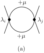
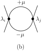
In general, we then find that the RG flow of the four-quark couplings is governed by two classes⁷⁷ 7 The two classes contain diagrams which are associated with contributions longitudinal and transversal to the heat bath. of one-particle irreducible (1PI) diagrams, see Fig. 1. These diagrams can be recast into so-called threshold functions which describe the decoupling of massive modes and modes in a thermal and/or dense medium. The definitions of these functions can be found in Ref. [10].

Let us now give a detailed discussion of the scale-fixing procedure underlying our calculations in this work. The values of the ten four-quark couplings at the initial RG scale $k=\Lambda$ can be considered as free parameters of our model. To pin them down, let us consider RG studies of QCD where the strengths of pointlike gluon-induced four-quark interactions have been analyzed in detail in the vacuum limit within a Fierz-complete setting [39, 40, 41]. There, it was found that the scalar-pseudoscalar channel $\mathcal{L}_{(\sigma\text{-}\pi)}$ is generated predominantly at high momentum scales $p\sim k$. Moreover, it was found that this channel remains to be the most dominant one over a wide range of scales down to $k\gtrsim 1\,\text{GeV}$, i.e. the modulus of any other four-quark coupling remains smaller than the one of the scalar-pseudoscalar coupling. With respect to our present study, it is also reasonable to expect that effects associated with an explicit breaking of Poincaré and $\mathcal{C}$ invariance are subleading as long as $T/k\ll 1$ and $\mu/k\ll 1$. In the light of these facts, we only choose the scalar-pseudoscalar coupling $\bar{\lambda}_{\text{($\sigma$-$\pi$)}}$ to be finite at the initial RG scale $\Lambda$ and set all other four-quark couplings to zero. Thus, at the initial scale, we are left with the action $S$ given in Eq. (1), $\Gamma_{k=\Lambda}=S$. This implies that we assume the $U_{\text{A}}(1)$ symmetry to be broken explicitly at the initial RG scale.⁸⁸ 8 In Subsec. IV.3, we discuss the effect of $U_{\text{A}}(1)$ symmetry breaking in more detail with the aid of the sum rules (17) and (18). Clearly, these considerations do not represent a rigorous determination of the initial conditions of our NJL-type model from QCD, which would require the dynamical inclusion of gauge degrees of freedom in an RG study [34, *Braun:2005uj, *Braun:2006jd, *Braun:2014wja, 39, 40, 42], but rather serve as a motivation for our scale-fixing procedure below.

The initial condition of the remaining coupling, the scalar-pseudoscalar coupling $\bar{\lambda}_{\text{($\sigma$-$\pi$)}}$, can be fixed in different ways. For example, we may tune it in the vacuum limit such that the resulting symmetry breaking scale $k_{\rm cr}$ leads to a given value for the critical temperature at vanishing chemical potential [10]. In the following, however, we employ a different procedure which exploits the mean-field gap equation for the chiral order-parameter field in a scalar-pseudoscalar one-channel approximation. To be more specific, performing a Hubbard-Stratonovich transformation of the path integral defined by the action (1) and integrating out the quark degrees of freedom subsequently, we arrive at a path integral over the auxiliary fields $\sigma\sim(\bar{\psi}\psi)$ and $\vec{\pi}\sim(\bar{\psi}\gamma_{5}\vec{\tau}\psi)$, respectively. From an evaluation of the latter in the mean-field approximation, we then obtain the following implicit equation for the constituent quark mass $\bar{m}_{\rm q}^{2}=\langle\sigma\rangle^{2}$ at $T=\mu=0$:⁹⁹ 9 From now on, we identify $\bar{\lambda}^{(\text{UV})}_{(\sigma\text{-}\pi)}$ with the value of the coupling $\bar{\lambda}_{(\sigma\text{-}\pi)}$ appearing in the classical action since the latter determines the value of this coupling at the UV scale $\Lambda$ in our RG study below.

where $\lambda_{\text{($\sigma$-$\pi$)}}^{\text{UV}}=\Lambda^{2}\bar{\lambda}_{(\sigma\text{-}\pi)}^{(\text{UV})}$ and $\lambda_{\text{($\sigma$-$\pi$)}}^{\ast}\equiv\lambda_{\text{($\sigma$-$\pi$)}}^{\ast}[r_{\psi}]$ is a dimensionless functional of the regularization scheme since $\mathcal{J}$ is not only a function of $\bar{m}_{\rm q}$ but also a functional of the so-called regulator shape function $r_{\psi}$ specifying the regularization scheme:

see also Ref. [8] for details. Diagrammatically, this integral is associated with a purely fermionic loop integral evaluated at vanishing external momenta.¹⁰¹⁰ 10 Loosely speaking, the loop integral corresponds to the diagram shown in the left panel of Fig. 1 with amputated external fermionic legs. The parameter $\Lambda$ may be considered a UV cutoff scale for the loop-momentum integral. However, from our RG standpoint, it should be rather associated with the initial RG scale at which we fix the initial conditions of the four-quark couplings in our RG study below.

For a given regularization scheme, the functional $\lambda_{\text{($\sigma$-$\pi$)}}^{\ast}$ determines the critical value of the four-quark coupling above which the ground state is governed by a finite vacuum expectation value $\langle\sigma\rangle\neq 0$. We find

Thus, we have $\bar{m}_{\rm q}>0$ for $\lambda_{\text{($\sigma$-$\pi$)}}^{\text{UV}}>\lambda_{\text{($\sigma$-$\pi$)}}^{\ast}$ and $\bar{m}_{\rm q}=0$ otherwise. For example, we obtain ${\lambda_{\text{($\sigma$-$\pi$)}}^{\ast}}=2\pi^{2}/N_{\rm c}$ for the four-dimensional sharp cutoff often employed in mean-field calculations and ${\lambda_{\text{($\sigma$-$\pi$)}}^{\ast}}=4\pi^{2}/N_{\rm c}$ for the Litim regulator [43, *Litim:2001up, *Litim:2001fd]. From here on, however, we shall employ the same scheme as in our studies of the RG flow of four-quark couplings to ensure comparability, see App. A for details. For this scheme, we find ${\lambda_{\text{($\sigma$-$\pi$)}}^{\ast}}=2\pi^{2}/N_{\rm c}$. In any case, we deduce from Eq. (19) that the actual value of ${\lambda_{\text{($\sigma$-$\pi$)}}^{\ast}}$ is of no importance. For a given regularization scheme together with a specific choice for the UV scale $\Lambda$, the quark mass $\bar{m}_{\rm q}$ only depends on the “strength” $\Delta\lambda_{\text{($\sigma$-$\pi$)}}$ of the scalar-pseudoscalar coupling relative to its critical value for chiral symmetry breaking:

In the following, we shall fix the scale in our studies by setting $\bar{m}_{\rm q}\approx 0.300\,\text{GeV}$ for the constituent quark mass in order to relate our model study to QCD. In terms of the scalar-pseudoscalar coupling, this choice corresponds to $\Delta\lambda_{\text{($\sigma$-$\pi$)}}\approx 0.234$ for $\Lambda/\bar{m}_{\rm q}\approx 10/3$.

From this discussion it follows immediately that a specific choice for $\Delta\lambda_{\text{($\sigma$-$\pi$)}}$ also determines the sign of the curvature $\bar{m}^{2}$ of the order-parameter potential $U$ at the origin. Indeed, we have

implying that, at the “critical point” $\Delta\lambda_{\text{($\sigma$-$\pi$)}}=0$, the curvature $\bar{m}^{2}$ of the order-parameter potential changes its sign. From the underlying Hubbard-Stratonovich transformation, we deduce that the renormalized scalar-pseudoscalar coupling $\bar{\lambda}_{(\sigma\text{-}\pi)}$ is inverse proportional to the curvature $\bar{m}^{2}$:

Thus, the scalar-pseudoscalar four-quark coupling diverges at the “critical point” $\Delta\lambda_{\text{($\sigma$-$\pi$)}}=0$.

As discussed on more general grounds in Subsec. III.1, these observations regarding the critical behavior and the formation of a non-trivial ground state can be carried over to studies of the RG flow of four-quark interactions, even beyond the mean-field limit. We refer the reader to Ref. [8] for a corresponding detailed discussion where it has also been shown that the value of $\lambda_{\text{($\sigma$-$\pi$)}}^{\ast}$ in the mean-field approximation is indeed nothing but the value of the non-Gaußian fixed-point of the scalar-pseudoscalar coupling in the large-$N_{\rm c}$ limit. Thus, this non-Gaußian fixed-point separates a regime governed by a trivial ground state from one governed by spontaneous symmetry breaking.

Let us now exploit the relation between the order-parameter potential and the RG flow of four-quark couplings to fix the scale in our study of the phase diagram below. To be specific, we first consider the flow equation for the dimensionless scale-dependent renormalized scalar-pseudoscalar coupling $\lambda_{\text{($\sigma$-$\pi$)}}=Z_{(\sigma\text{-}\pi)}k^{2}\bar{\lambda}_{\text{($\sigma$-$\pi$)}}/(Z^{\perp})^{2}$ in the one-channel approximation at $T=\mu=0$:

Here, we have employed the regularization scheme defined in App. A which is identical to the well-known four-dimensional exponential scheme in the vacuum limit [46, 47], see Ref. [48] for a detailed discussion of regularization schemes in RG studies. The flow equation (25) has been extracted from the set of equations for the Fierz-complete basis of four-quark interactions given in App. B by setting all couplings but the scalar-pseudoscalar coupling to zero and also dropping their flow equations. Note that, because of the Fierz ambiguity, the flow equation (25) is ambiguous in the sense that the prefactor of the term quadratic in the four-quark coupling is not unique.

The flow equation (25) has two fixed points: a Gaußian fixed point and the before-mentioned non-Gaußian fixed point $\lambda_{\text{($\sigma$-$\pi$)}}^{\ast}$,

Thus, the value of the non-Gaußian fixed point indeed agrees with the critical value of the scalar-pseudoscalar coupling in the mean-field approximation for $N_{\rm c}\gg 1$. Again, with respect to the question of the formation of a non-trivial ground state, the actual value of the non-Gaußian fixed point is of no importance, only the value of the scalar-pseudoscalar coupling at the initial RG scale $\Lambda$ relative to the value of the non-Gaußian fixed point matters. Choosing $\lambda_{\text{($\sigma$-$\pi$)}}^{(\text{UV})}>\lambda_{\text{($\sigma$-$\pi$)}}^{\ast}$, we find that the scalar-pseudoscalar coupling diverges at a finite scale $k_{\text{cr}}$,

indicating the onset of chiral symmetry breaking, i.e. the curvature of the order-parameter at the origin changes its sign at this so-called chiral symmetry breaking scale $k_{\text{cr}}$. This scale sets the scale for the (chiral) low-energy observables, such as the constituent quark mass $\bar{m}_{\rm q}\sim k_{\text{cr}}$. Using the relation (27), we can compute the value of the chiral symmetry breaking scale in the mean-field approximation. Using $\Delta\lambda\approx 0.234$ extracted from the mean-field calculation above for $\bar{m}_{\rm q}\approx 0.300\,\text{GeV}$ and $\Lambda/\bar{m}_{\rm q}\approx 10/3$, we obtain $k_{0}/\bar{m}_{\rm q}\equiv k_{\text{cr}}/\bar{m}_{\rm q}\approx 1.613$, where $k_{0}$ serves as a reference scale in the remainder of this work.

At first glance, it seems that Eq. (27) defining $k_{\text{cr}}$ implies that the low-energy dynamics is independent of the combinatoric prefactor of the term quadratic in the four-quark coupling in Eq. (25). However, this turns out to be too naive. A closer look reveals that the contribution $\sim 1/N_{\rm c}$ is related to quantum corrections to the Yukawa coupling in a partially bosonized formulation of our model [49, 8]. In a study of the partially bosonized formulation, these corrections therefore yield $1/N_{\rm c}$-corrections to the critical scale $k_{\text{cr}}$. Moreover, it should be noted that order-parameter fluctuations, which are nothing but $1/N_{\rm c}$-corrections, tend to restore the chiral symmetry in the infrared limit, thereby lowering the value of the critical temperature compared to its value in the large-$N_{\rm c}$ approximation (see, e.g., Ref. [50]).

At the order of the derivative expansion considered in this work, we do not have access to low-energy observables such as the constituent quark mass, see our discussion in Subsec. III.1. Therefore, we exploit the relation between the chiral order-parameter potential in the mean-field approximation and the RG flow of the corresponding scalar-pseudoscalar coupling to fix the scale in our calculations. In all our studies of the phase diagram presented below, we shall set all four-quark couplings to zero at the initial RG scale $\Lambda$ except for the scalar-pseudoscalar coupling $\lambda_{\text{($\sigma$-$\pi$)}}$. The latter is tuned at this scale such that, at $T=\mu=0$, we obtain $k_{\text{cr}}=k_{0}$, i.e. the value of the critical scale is always tuned to agree identically with its value in the mean-field approximation. This ensures comparability between the results of our studies from different approximations. Moreover, since $k_{0}$ is directly related to the constituent quark mass in the mean-field approximation, $k_{0}/\bar{m}_{\rm q}\approx 1.613$, this allows at least for a rough translation of our results for the phase transition temperatures as obtained from, e.g., our Fierz-complete set of flow equations into physical units. Of course, such a translation is only approximative. We always have to keep in mind that the use of the same value for $k_{0}$ in different approximations may not necessarily translate into the same value for the low-energy observables, such as the constituent quark mass. In any case, considering the critical temperature at $\mu=0$ as an example for an low-energy observable being sensitive to the vacuum constituent quark mass and also accessible within our framework, we find that this quantity does not depend strongly on our approximations associated with different numbers of four-quark channels. This observation may be traced back to the fact that we find the scalar-pseudoscalar channel to be most dominant at $\mu=0$, therefore governing the low-energy dynamics in this regime, see our discussion below.

Let us now study the phase diagram in the plane spanned by the temperature and quark chemical potential for an approximation in which we only take into account the scalar-pseudoscalar four-quark coupling. The flow equation of the latter reads:

where $v_{4}=1/(32\pi^{2})$, $\tau=T/k$, and $\tilde{\mu}_{\tau}=\mu/(2\pi T)=\mu/(2\pi k\tau)$. Here and in the following, we do not take into account the renormalization of the chemical potential and set $Z_{\mu}=1$. The definitions of the so-called threshold functions also mentioned in Subsec. III.1 can be found in Ref. [10]. The ones appearing in Eq. (28) are associated with the loop integral depicted in the left panel of Fig. 1. As done for Eq. (25), we have extracted the flow equation (28) from the set of equations for the Fierz-complete basis of four-quark interactions given in App. B by setting all but the scalar-pseudoscalar coupling to zero and also dropping their RG flow equations. In the limit $T\to 0$ and $\mu\to 0$, we therefore recover Eq. (25) from Eq. (28) since

for $T\to 0$ and $\mu\to 0$, see Ref. [10].

The flow equation (28) can be solved analytically, even at finite temperature and quark chemical potential [10]. The solution can then be employed to compute the critical temperature $T_{\rm cr}=T_{\rm cr}(\mu)$ as a function of the quark chemical potential $\mu$. The latter is defined as the temperature at which the scalar-pseudoscalar four-quark coupling still diverges at $k\to 0$:

i.e. it is defined as the highest temperature for which the four-quark coupling still diverges. For our studies with more than one channel, this definition can be generalized straightforwardly. The critical temperature is then defined to be the temperature at which the four-quark couplings diverge. Note that a divergence in one channel at a scale $k_{\text{cr}}(T,\mu)$ entails corresponding divergences in all the other channels at the same scale. However, the associated four-quark couplings in general have a different strength relative to each other, see, e.g., Subsec. IV.2 below and also Ref. [10] for a detailed discussion.

With the definition (30), we obtain the following implicit equation for the critical temperature $T_{\rm cr}$:

For convenience, we have introduced the following dimensionless auxiliary function:

where $\tau^{\prime}=T/k^{\prime}$.

Apparently, the critical temperature $T_{\text{cr}}$ depends on our choice for the UV scale $\Lambda$ as well as the scale $k_{0}$, i.e. eventually on the constituent quark mass in the vacuum limit. Recall that the scale $k_{0}$ is directly related to the initial condition for the scalar-pseudoscalar four-quark coupling which we keep fixed to the same value for all temperatures and chemical potentials. In the following, we shall therefore measure all physical observables in units of $k_{0}$.

In Fig. 2, we show the critical temperature as a function of the quark chemical potential for the one-channel approximation (gray line) as obtained from a solution of Eq. (31). For $\mu=0$, we obtain $T_{\text{cr}}/k_{0}\approx 0.390$ ($T_{\text{cr}}\approx 0.190\,\text{GeV}$). For increasing $\mu$, the critical temperature then decreases monotonously and eventually vanishes at $\mu/k_{0}=\mu_{\text{cr}}/k_{0}\approx 1.14$ ($\mu_{\text{cr}}\approx 0.552\,\text{GeV}$).

We emphasize again that our definition of the critical temperature is associated with a sign change of the chiral order-parameter potential at the origin. In our present approximation, our result for $T_{\text{cr}}(\mu)$ therefore only describes the phase boundary in case of a second-order transition. Our criterion is not sensitive to a first-order transition. However, it allows to detect the line of metastability separating a regime associated with a negative curvature of the order-parameter potential at the origin (e.g. at low temperature and small quark chemical potential) from a regime where the curvature changes its sign but the true ground state is still assumed for a finite expectation value of the order-parameter field. Such lines of metastability usually emerge in the vicinity of a first-order transition. In particular, for a given temperature, the chemical potential associated with the emergence of a metastable state at the origin of the potential is less or equal than the chemical potential of the associated first-order transition.

It is instructive to compare the results for the phase boundary from our RG study with those obtained from a solution of the mean-field gap equation (19).¹¹¹¹ 11 The gap equation for finite $T$ and $\mu$ is obtained from Eq. (19) by replacing $\int{\rm d}^{4}p/(2\pi)^{4}$ with $T\sum_{n}\int{\rm d}^{3}p/(2\pi)^{3}$. Moreover, we have to replace $p^{2}$ with $(\nu_{n}^{2}-{\rm i}\mu)^{2}+\vec{p}^{\,2}$, where $\nu_{n}=(2n+1)\pi T$, except in the argument of the regulator shape function due to our conventions. To ensure comparability, we employ of course the same regularization scheme as in our RG study. We then find that the phase transition line from our RG study agrees identically with the second-order phase transition line of the mean-field study up to a first-order endpoint at $(\mu/k_{0},T/k_{0})\approx(0.951,0.207)$. As expected, beyond this point, the phase transition line obtained from our RG study agrees identically with the line of metastability in the mean-field phase diagram. The comparatively large extent of the phase boundary in $\mu$-direction can be traced back to the comparatively large $\sigma$-meson mass $\bar{m}_{\sigma}/\bar{m}_{\rm q}\approx 2.67$ ($\bar{m}_{\sigma}\approx 0.800\,\text{GeV}$) found in the vacuum limit of our mean-field calculation for the employed set of parameters, i.e. $\Delta\lambda_{\text{($\sigma$-$\pi$)}}$ and $\Lambda$.¹²¹² 12 The computation of the $\sigma$-mass requires fixing the Yukawa coupling $\bar{h}$ since $m_{q}=\langle\sigma\rangle=\bar{h}f_{\pi}$. Here, we use $\bar{h}\approx 3.45$ corresponding to $f_{\pi}\approx 87.0\,\text{MeV}$ for the pion decay constant. In fact, it has already been found in previous mean-field calculations that the critical point separating a first-order phase transition line from a second-order phase transition line can be shifted continuously to larger values of the quark chemical potential by increasing the mass of the $\sigma$-meson [51]. Even more, it can even be made disappear, leaving us with only a second-order transition line. Note that this highlights the strong scheme dependence as the $\sigma$-mass can be tuned by suitable variations of the constituent quark mass and the UV cutoff $\Lambda$. Since the actual value of the latter should always be viewed against the background of the employed regularization scheme, the scheme unavoidably belongs to the definition of the model, at least in four Euclidean space-time dimensions. Of course, we could also use smaller values for $\Lambda$ which would lead to a smaller mass of the $\sigma$-meson. However, this then leads to strong “cutoff effects” as both the temperatures as well as the quark chemical potentials considered in this work would then be of the order of the UV scale $\Lambda$. In order to at least suppress such unwanted effects, we have chosen $\Lambda/k_{0}\approx 2.07$.

Let us now analyze the phase diagram as obtained from an RG flow study of the Fierz-complete set of four-quark interactions, see App. B for the RG flow equations. Such an analysis goes well beyond studies in the mean-field limit. Indeed, mean-field studies of NJL-type low-energy models have been found to exhibit a residual ambiguity related to the possibility to perform Fierz transformations, even if a Fierz-complete set of four-quark interactions is taken into account [52], see also Ref. [53] for an introduction. Results from mean-field calculations therefore potentially depend on an unphysical parameter which reflects the actual choice of the mean field in the various channels.

As discussed above, we fix the scale in our Fierz-complete studies by setting all but the scalar-pseudoscalar coupling to zero at the initial RG scale $\Lambda$. The latter is tuned at $T=\mu=0$ such that the critical scale $k_{0}$ associated with diverging four-quark couplings agrees identically with its counterpart in the mean-field calculation. For our calculations at finite temperature and/or quark chemical potential, we then use the same set of initial conditions as in the vacuum limit, i.e. at $T=\mu=0$. The scale dependence of the (dimensionful) renormalized four-quark couplings at $T=\mu=0$ is shown in Fig. 3. We observe that the dynamics of the theory in this case is clearly dominated by the scalar-pseudoscalar interaction channel; the modulus of all other couplings is at least one order of magnitude smaller than the modulus of the scalar-pseudoscalar coupling. The dominance of this channel may indicate that the ground state in the vacuum limit is governed by chiral symmetry breaking. However, we emphasize again that such an analysis based on the strength of four-quark interactions has to be taken with some care: It neither rules out the possible formation of other condensates associated with subdominant channels nor proves the formation of a condensate associated with the most dominant channel. Such an analysis can only yield indications for the actual structure of the ground state, see Ref. [10] for a detailed discussion.

In the vacuum limit, the observation of the dominance of the scalar-pseudoscalar channel may be considered trivial as it may be exclusively triggered by our choice for the initial conditions. Increasing now the temperature at vanishing quark chemical potential, we still observe a dominance of the scalar-pseudoscalar channel which persists even up to high temperatures beyond the critical temperature $T_{\text{cr}}(\mu=0)/k_{0}\approx 0.391$. This is illustrated in the left panel of Fig. 4 where the scale dependence of the various four-quark couplings is shown for $T\simeq T_{\text{cr}}(\mu\!=\!0)$ at $\mu=0$. At least in units of $k_{0}$, it also appears that the critical temperature at $\mu=0$ in our Fierz-complete study agrees very well with the one from the one-channel approximation. However, we note that this could be misleading as choosing the same value for $k_{0}$ in our Fierz-complete study and in our one-channel approximation may not necessarily lead to the same values of the low-energy observables (e.g. the constituent quark mass), although the flow in the vacuum limit is also strongly dominated by the scalar-pseudoscalar channel in the Fierz-complete analysis. Thus, direct quantitative comparisons of the results from our various different approximations should be taken with care. Still, we expect that qualitative comparisons are meaningful.

Following now the critical temperature $T_{\text{cr}}$ as a function of $\mu$ starting from $\mu=0$, we find that the scalar-pseudoscalar channel continues to dominate the dynamics up to $\mu/k_{0}=\mu_{\chi}/k_{0}\approx 0.734$, as depicted by the blue solid line in Fig. 2. In this regime, we also observe that the phase transition temperatures from our one-channel approximation agree almost identically with those from the Fierz-complete study, at least in units of the vacuum symmetry breaking scale $k_{0}$.¹³¹³ 13 Note that $\mu_{\chi}/k_{0}\approx 0.734$ roughly corresponds to $\mu_{\chi}/\bar{m}_{\rm q}\approx 1.18$ in our mean-field approximation, where $\bar{m}_{\rm q}\approx 0.3\,\text{GeV}$. At first glance, this may come as a surprise. We shall therefore analyze this observation in detail in Subsec. IV.4 below. Following the phase transition line beyond the point associated with the quark chemical potential $\mu_{\chi}$, we find that the dynamics is now clearly and exclusively dominated by the CSC (color superconducting) channel associated with the emergence of a diquark condensate $\delta^{a}$ and a corresponding gap in the quark propagator, see blue dashed line in Fig. 2. Exemplary, this change in the “hierarchy” of the channels is illustrated in the right panel of Fig. 4 where the scale dependence of the various four-quark couplings is shown for $\mu/k_{0}\approx 1.1$ and $T/k_{0}\gtrsim T_{\text{cr}}(\mu)/k_{0}\approx 0.196$. We emphasize that this change in the “hierarchy” of the channels is non-trivial as it is fully triggered by the dynamics of the system when the quark chemical potential is increased. There is no fine-tuning of, e.g., the CSC coupling involved. Recall that we use identical initial conditions in the vacuum limit as well as at finite temperature and/or quark chemical potential.

Our choice for the initial conditions of the RG flow equations explicitly breaks the $U_{\rm A}(1)$ symmetry since we only choose the coupling $\lambda_{\text{($\sigma$-$\pi$)}}$ to be finite and set all the other four-quark couplings to zero at the initial RG scale $\Lambda$. By using the sum rules (17) and (18), we can now study the fate of the (broken) $U_{\rm A}(1)$ symmetry at finite temperature and quark chemical potential when quantum fluctuations are taken into account. To be specific, in case of $U_{\rm A}(1)$-violating initial conditions, we consider the following two dimensionless quantities to “measure” the strength of the explicit $U_{\rm A}(1)$ symmetry breaking:

The normalization $\mathcal{N}$ is chosen to be independent of the index $i$ and is implicitly determined by

Thus, the auxiliary quantities defined in Eq. (33) essentially measure the strength of $U_{\rm A}(1)$ symmetry breaking relative to its strength at the initial RG scale $\Lambda$. In case of a $U_{\rm A}(1)$-symmetric theory defined by a suitable choice for the initial conditions, we find that the couplings fulfill the sum rules (17) and (18) at all scales $k$ greater than the symmetry breaking scale, as it should be. Therefore, there is no need at all to consider the auxiliary quantities defined in Eq. (33) in such a scenario.

In Fig. 5, we show the scale dependence of $R_{1}$ and $R_{2}$ for two values of the quark chemical potential, $\mu=0$ and $\mu/k_{0}\approx 1.1$, and three values of the temperature for each of the two cases as obtained for our $U_{\rm A}(1)$-violating initial conditions. Let us first note that, for all values of $\mu$ considered in this work, we observe that $U_{\rm A}(1)$ breaking as “measured” by our sum rules in form of $R_{1}$ and $R_{2}$ is continuously softened when the temperature is increased. More specifically, at $\mu=0$, for example, we already find that the strength of $U_{\rm A}(1)$ breaking remains on the level of its strength at the initial scale $\Lambda$ for temperatures $T/T_{\text{c}}\gtrsim 2$, i.e. its strength remains on the level as present in the classical action in this temperature regime. A qualitatively similar behavior can also be observed at finite chemical potential when the temperature is increased, see Fig. 5. Indeed, the strength of $U_{\rm A}(1)$ symmetry breaking is controlled by the strength of the four-quark couplings. Quantum corrections to the latter are thermally suppressed at high temperature due to the presence of a thermal mass of the fermions. This explains our observations at high temperature.

Conversely, approaching the phase transition from above for a given value of the chemical potential $\mu$, we find that the violation of the $U_{\rm A}(1)$ symmetry becomes continuously stronger, in the sense that the functions $R_{1}$ and $R_{2}$ start to increase, eventually deviating significantly from their values at the initial RG scale. Thus, quantum corrections to the four-quark couplings appear to amplify $U_{\rm A}(1)$ symmetry breaking when the phase governed by spontaneous symmetry breaking is approached from above, provided that $U_{\rm A}(1)$ symmetry breaking is explicitly broken at the initial RG scale.

In accordance with our observation that the scalar-pseudoscalar channel is most dominant at small chemical potential (see, e.g., left panel of Fig. 4), we also note that $R_{2}\gg R_{1}$ in this part of the phase diagram, see left panel of Fig. 5. For $\mu\gtrsim\mu_{\chi}$, the CSC channel then dominates the dynamics and thus $R_{1}$ and $R_{2}$ are of the same order of magnitude as both depend on the CSC coupling, see the right panels of Figs. 4 and 5. Thus, our results suggest that the dynamically generated violation of the $U_{\rm A}(1)$ symmetry is driven by the dynamics of the pions at small chemical potential whereas it is driven by the dynamics of diquark degrees of freedom associated with the CSC channel at large chemical potential.

Let us finally compare the phase diagram obtained from our Fierz-complete study employing $U_{\rm A}(1)$-symmetry violating initial conditions with the one obtained from a manifestly $U_{\rm A}(1)$-symmetric Fierz-complete study. The latter has been calculated by tuning the couplings $\bar{\lambda}_{\text{($\sigma$-$\pi$)}}$ and $\bar{\lambda}_{(S+P)_{-}}$ at the initial RG scale such that the sum rule (18) is fulfilled and the same value for the symmetry scale $k_{0}$ as in the case with $U_{\rm A}(1)$-symmetry violating initial conditions is obtained in the vacuum limit. If we choose the initial conditions in this way, i.e. such that they respect the $U_{\rm A}(1)$ symmetry, then this symmetry remains intact in the RG flow for all values of the RG scale, at least for those values of the temperature and the quark chemical potential for which the four-quark couplings remain finite on all scales $k\leq\Lambda$. For values of the temperature and the quark chemical potential at which the four-quark couplings diverge at a finite scale $k_{\text{cr}}(T,\mu)$, the sum rules (17) and (18) are only fulfilled for $k>k_{\text{cr}}(T,\mu)$. Below the symmetry breaking scale, the $U_{\rm A}(1)$ symmetry may potentially be broken spontaneously, e.g. alongside with the chiral symmetry. However, this cannot be resolved in our present study.

As already discussed above, a quantitative comparison of the results from our $U_{\rm A}(1)$-symmetric calculation with the ones from our explicitly $U_{\rm A}(1)$-violating calculation is generically difficult and has to be taken with some care. Leaving this concern aside for a moment, we observe that the phase transition lines from both studies agree almost identically on the scale of the plot. Only for larger values of the quark chemical potential, we find that the two phase transition lines start to deviate from each other. In particular, we observe that, along the phase transition line, a chemical potential $\mu_{\chi}/k_{0}$ associated with a change in the hierarchy of the four-quark couplings exists in both cases. Even the corresponding values of $\mu_{\chi}/k_{0}$ agree almost identically. Even more, for $\mu<\mu_{\chi}$, we find that the scalar-pseudoscalar channel dominates the dynamics of the theory in both cases, see solid lines in Fig. 6. For $\mu>\mu_{\chi}$, the dynamics is then dominated by the CSC channel in case of $U_{\rm A}(1)$-symmetry violating initial conditions, see blue dashed line in Fig. 6. In case of our $U_{\rm A}(1)$-symmetric study, however, we have a dominance of the ${(V+A)_{\parallel}^{\mathrm{adj}}}$-channel in this regime as depicted by the red dashed-dotted line in Fig. 6; see Eq. (11) for the definition of this channel. The condensate associated with this channel also breaks the color symmetry of our theory. In mean-field studies (see, e.g., Ref. [5] for a review), the appearance of a corresponding condensate has also been discussed. However, its generation has been found to be induced by a simultaneous formation of a color-symmetry breaking diquark condensate. In accordance with this, we observe that the four most dominant channels along the phase transition line for $\mu>\mu_{\chi}$ are the ${(V+A)_{\parallel}^{\mathrm{adj}}}$-, $(S+P)_{-}^{\mathrm{adj}}$-, CSC- and ${(V-A)_{\perp}^{\mathrm{adj}}}$-channel in our present study. These channels are all associated with the formation of a color-symmetry breaking condensate. Apart from the $(V\pm A)_{\parallel}$-channels, color-singlet channels are found to be subdominant in this part of the phase diagram. The observed difference in the dominance pattern at large chemical potential in the $U_{\rm A}(1)$-symmetric and $U_{\rm A}(1)$-violating calculation may point to the importance of explicit $U_{\rm A}(1)$ breaking for the formation of the conventional CSC ground state at intermediate and large values of the chemical potential as discussed in early seminal works on color superconductivity, see, e.g., Refs. [24, 25, 54, 55, *Pisarski:1999tv, *Pisarski:1999bf, *Schafer:1999jg, *Brown:1999aq, *Hong:1999fh, *Evans:1999at].

By simply looking at the shape of the phase boundary, one may be tempted to conclude that $U_{\rm A}(1)$ breaking does not strongly affect the position of the phase transition line. However, this may be a too bold statement at this point as the same value of $k_{0}$ in the two studies potentially corresponds to different values of the low-energy observables and therefore renders a direct quantitative comparison difficult, see our discussion above. In any case, the apparent insensitivity of the phase transition line under a “transition” from $U_{\rm A}(1)$-symmetry violating initial conditions to $U_{\rm A}(1)$-symmetric initial conditions (while keeping the vacuum symmetry breaking scale fixed) is still an interesting observation. At least at small values of the chemical potential, the latter can in principle be understood from an analysis of the large-$N_{\rm c}$ limit which we shall consider next.

In order to better understand the phase structure at small chemical potential, we now analyze our RG flow equations in the large-$N_{\rm c}$ limit, i.e. we only take into account the leading order of the right-hand sides of our flow equations in an expansion in powers of $N_{\rm c}$. For the scalar-pseudoscalar coupling, for example, we then obtain

For the remaining nine four-quark couplings, we find that the right-hand sides of their flow equations do not contain terms quadratic in the scalar-pseudoscalar coupling $\lambda_{\text{($\sigma$-$\pi$)}}$ but at most terms linear in $\lambda_{\text{($\sigma$-$\pi$)}}$ in the large-$N_{\rm c}$ limit. At first glance, this may not appear noteworthy. However, by setting all four-quark couplings but the scalar-pseudoscalar coupling to zero on the right-hand sides of the flow equations, we therefore observe that only the right-hand side of the flow equation of the scalar-pseudoscalar coupling remains finite. Indeed, from Eq. (35), we deduce that

Note that this flow equation is identical to Eq. (28) in the large-$N_{\rm c}$ limit.