Analysis and Design of Serially Concatenated LDGM Codes

Concatenated codes [1] were first introduced by David Forney in 1965. These codes employ two stages of encoding and decoding [1, 2] as shown in Fig. 1. During encoding, the original information bits are first encoded using an outer code to produce intermediate bits which are further encoded using an inner code to produce final output bits that are transmitted over a communication channel. During decoding, first, the decoding of the inner code is conducted followed by the decoding of the outer code. Serially concatenated low-density generator-matrix (SCLDGM) codes that use the same two-stages of encoding and decoding are proposed in [3]. Although single LDGM codes are asymptotically bad [3], the SCLDGM codes are shown to have impressive performance comparable to turbo and LDPC codes over noisy channels under sum-product (SP) decoding [3, 4, 5].

Both the inner and outer codes of the SCLDGM code use SP algorithm, also known as belief propagation (BP) algorithm, as the decoding method. The behaviour of the SP decoding can be exactly tracked using density evolution (DE) [6] or its discretized version called discretized density evolution (DDE) [7]. A DE approximation algorithm known as Gaussian approximation (GA) method [7] and extrinsic information transfer (EXIT) functions [8] are also popularly used for analysing such codes that use SP decoding [5, 9, 4, 10]. In [3], only simulation results are used to show that the SCLDGM codes perform close to the Shannon limit, however, no asymptotic analysis are presented for binary input additive white Gaussian noise (BIAWGN) channels. Asymptotic analysis of the single LDGM codes and the parallel concatenated LDGM codes are presented in [5]. In [9], considering single LDGM codes two formulas are presented for the prediction of the error floor. EXIT functions are used in [4, 9] to design better SCLDGM codes and provide their decoding thresholds. However, none of these works presented the exact asymptotic curves for the SCLDGM codes using the DDE. Since both the inner and outer decoders of SCLDGM codes use the SP decoding, it is possible to asymptotically analyse these codes using the DDE. Therefore, by applying the DDE to the inner code and then to the outer code, in this paper, we first provide the exact asymptotic curves and the decoding thresholds of the SCLDGM codes. Such DDE implementation for the concatenated codes termed as two-step DDE has been successfully developed and used in [11, 12] to asymptotically analyse another class of concatenated codes known as physical layer Raptor codes [13] and their systematic version.

Forney described [1] that the only function of the inner decoder is to bring the probability of decoding error to the range of $10^{-2}\sim 10^{-4}$, which once achieved, the outer decoder further drives the overall probability of decoding error down to an extremely small desired value. More specifically, that range for BIAWGN channel is predicted to be $10^{-2}\sim 10^{-3}$ [1]. Finding the exact value in that range is crucial for designing optimal concatenated codes. In this paper, for SCLDGM codes in BIAWGN channels that use the SP decoding algorithm, we provide the exact probability of decoding error, termed as critical bit error rate (BER), that an inner decoder should at least produce for the successful decoding of these codes. It also means that successful decoding is impossible if the decoding is handed to the outer decoder before the critical BER is achieved by the inner decoder. This necessary condition for successful decoding leads to a conclusion that in fact the overall decoding threshold of a concatenated code is the minimum $E_{b}/N_{o}$ at which the inner decoder achieves the critical BER determined by the outer code.

While LDGM codes are known to have poor decoding performance and bad error floors in BIAWGN channel [3], the SCLDGM codes greatly improve the decoding performance. The error-floors are drastically lowered, however, are not eradicated. In order to understand the error-floor behaviour of these codes, in this paper, we present a detailed error-floor analysis and provide the lower-bound formulas for both the LDGM and SCLDGM codes. For the SCLDGM codes, we show that our lower-bound formulas become the closest approximation of the exact asymptotic performance in the region beyond their decoding thresholds. We also study the asymptotic performance of another concatenation scheme where inner LDGM codes are serially concatenated with high-rate regular low-density parity-check (LDPC) codes. This code was introduced in [14] and termed as low-density parity-check and generator-matrix (LDPC-GM) code. It was shown that the LDPC-GM codes achieve capacity in binary erasure channel (BEC) under BP decoding. However, the exact asymptotic performance analysis of the LDPC-GM codes for BIAWGN channel that uses SP decoding using the DDE is still missing. Therefore, in this paper, we also provide the exact asymptotic curves of these codes using the two-step DDE method. Furthermore, we show that since the high-rate regular LDPC codes do not suffer from error-floors, its use as an outer code in the concatenated scheme can completely eradicate the error floors associated with LDGM codes, thus making the LDPC-GM codes error-floor-free capacity approaching codes for BIAWGN channels.

Density evolution based optimization approaches have been used to provide optimized LDPC codes with the best known decoding thresholds [7, 15]. For the concatenated codes with a known outer code, due to the knowledge of the critical BER, designing a good concatenated code boils down to finding an inner code that achieves the critical BER at the lowest possible $E_{b}/N_{o}$ [11]. This approach has been successfully used in [11] to optimally design physical layer Raptor codes. In this paper, we further use the critical BER-based DDE optimization approach to design an optimized SCLDGM code that performs close to the Shannon limit. We demonstrate the improved performance of our optimized SCLDGM code through both asymptotic and simulation results.

The rest of the paper is organized as follows. Section II presents the encoding and decoding of the SCLDGM codes. In Section III, we provide the details of DDE implementation for SCLDGM codes to obtain the exact asymptotic curves and the decoding thresholds. We also provide the necessary condition for the successful decoding and discuss the faster convergence behaviour of these codes. Section IV addresses the error-floor analysis of both the LDGM and SCLDGM codes along with the lower-bound formulas. In Section V, we present the exact asymptotic curves of the LDPC-GM codes. We further show that by using high-rate LDPC code as an outer code, the error floors of concatenated codes are completely eradicated. Section VI presents a capacity approaching optimized SCLDGM code designed using the critical BER-based DDE optimization approach. Finally, Section VII concludes the paper.

In the two-stage encoding of SCLDGM codes, at first, $k$ information bits are encoded using a high rate outer code to produce $k^{\prime}$ intermediate bits which are further encoded using an inner code to produce $n$ output bits. Hence, the code-rates of the outer and the inner codes are $r_{o}=k/k^{\prime}$ and $r_{i}=k^{\prime}/n$ respectively, making a SCLDGM code of code-rate $r=r_{i}r_{o}=k/n$. Let $\bm{s}=[s_{1},s_{2},\cdots,s_{k}]$ represent information bits. For a SCLDGM code, encoding at each stage is systematic. Therefore, the intermediate and output bits are $\bm{m}=[s_{1},s_{2},\cdots,s_{k},t_{1},\cdots,t_{k^{\prime}-k}]$ and $\bm{o}=[s_{1},s_{2},\cdots,s_{k},t_{1},\cdots,t_{k^{\prime}-k},p_{1},\cdots,p_{n-k^{\prime}}]$ respectively, where $\bm{t}=[t_{1},\cdots,t_{k^{\prime}-k}]$ and $\bm{p}=[p_{1},\cdots,p_{n-k^{\prime}}]$ represent outer and inner parity bits. Let $n_{i}$ and $n_{o}$ represent the number of inner and outer parity bits respectively. Thus, $n=k+n_{i}+n_{o}$. These output bits are first modulated and then transmitted over a channel to be collected and decoded at the receiver.

We consider transmission over the BIAWGN channel using binary phase shift keying (BPSK) modulation. This is modelled as $y=x+\eta$, where $x\in\{-1,+1\}$, $\eta$ is zero-mean Gaussian noise with $\sigma^{2}$ variance, and $y$ is the received corrupted bit. The channel estimate is calculated as $2y/\sigma^{2}$.

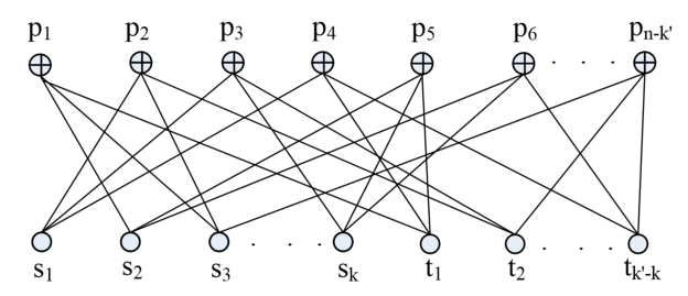
For the inner SP decoding, the bipartite graph as shown in Fig. 2(a) is used, where the inner parity bits $\left(\bm{p}=[p_{1},\cdots,p_{n-k^{\prime}}]\right)$ are used as check nodes (CNs) and intermediate bits $\left(\bm{m}=[s_{1},s_{2},\cdots,s_{k},t_{1},\cdots,t_{k^{\prime}-k}]\right)$ are used as variable nodes (VNs). It must be noted that in this bipartite graph, both VNs and CNs are transmitted through the noisy channel and hence both have initial channel estimates. This is unlike the bi-partite graph used in LDPC codes where CNs do not have channel estimates.

Under LDGM’s SP decoding, the updates from the $j$th CN to the $i$th VN denoted by $L_{c_{j}v_{i}}$ and from the $i$th VN to the $j$th CN denoted by $L_{v_{i}c_{j}}$ are computed as

where $L(v_{i})$ and $L(c_{j})$ represent the channel estimates of the corresponding VN and CN, respectively, and $N_{c}(j)$ denotes the set of VNs connected to the $j$th CN and $N_{v}(i)$ denotes the set of CNs connected to the $i$th VN.

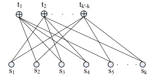
The inner SP decoding is conducted for some predefined number of iterations and then the final estimate of each VN is calculated using a decision rule $\left(L(v_{i})+\sum_{j\in N_{v}(i)}L_{c_{j}v_{i}}\right)$ that sums all the incoming messages also known as log-likelihood ratios (LLRs) and the channel estimate of the VN. These values are then used as the initial LLRs for the outer decoding. The decoding graph used for outer decoding is as shown in Fig. 2(b), where the outer parity bits are used as the CNs and the information bits are used as the VNs. After running SP decoding for the outer code over some predefined number of iterations, the final hard decision can be made for each VN based on the estimates calculated using the decision rule. We call such decoding where the decoding of the outer code is conducted only after completing the decoding of the inner code as two-step SP decoding.

Decoding of such concatenated codes can also be done using joint decoding in which both the inner and outer decoding are conducted at each iteration and then the process is repeated over a predefined number of global iterations. Therefore, unlike in the two-step decoding where the outer decoder gets extra information at the end of the decoding of inner decoder, in the joint decoding, both the inner and outer decoder exchange information at each iteration. However, since the outer code considered in the SCLDGM codes is of very high rate, the information provided by it to the inner decoder is less significant. Thus, not much improvement in the decoding performance is achieved, which is also depicted in Fig. 3. We see that at the BER level of $10^{-5}$, the joint decoding merely outperforms the two-step decoding by a margin of around $0.05$ dB. Hence, for our asymptotic and error-floor analysis of the SCLDGM codes, we only consider the two-step SP decoding, which also follows the decoding method in [3, 4].

It is known that the asymptotic behavior of the SP decoding can exactly be tracked using DE [6]. Both the inner and outer codes of SCLDGM codes use SP decoding. Hence, we first apply DDE to the inner code and then to the outer code to obtain the asymptotic curves of the SCLDGM codes. We assume that all-one BPSK symbols are transmitted. Therefore, the received LLRs (channel estimates) over a BIAWGN channel are known to be symmetric Gaussian distributed with mean $2/\sigma^{2}$ and variance $4/\sigma^{2}$, i.e., $\mathcal{N}\left(2/\sigma^{2},4/\sigma^{2}\right)$, where the variance is twice the mean and this symmetric condition has been proved to be preserved under the SP decoding [6]. The noise parameter $\sigma$, channel condition $E_{b}/N_{o}$, and the overall code-rate $r$ are related as $E_{b}/N_{o}=10\log_{10}\left(1/(2r\sigma^{2})\right)$.

Single LDGM codes are asymptotically bad and suffer from high error floors. The SCLDGM codes drastically improve the decoding performance and have decoding performance close to the Shannon limit. However, they still exhibit error-floor behaviour, although at the very lower BER level as shown in Fig. 5. In this section, we provide the reasons behind such error floors and give the lower bounds for both the single LDGM and SCLDGM codes. For this purpose, we have considered both the inner and outer LDGM codes as regular codes with VN degree $d_{v}$ and $d_{v}^{(o)}$ respectively.

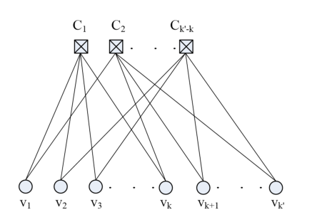
In the LDPC-GM codes, the high-rate LDPC codes are used as the outer codes. An LDPC code is defined by its parity check matrix $(H)$ which is used to construct its bi-partite decoding graph as shown in Fig. 11, where $k^{\prime}$ represent the length of the codeword produced by the LDPC encoding. Let $\bm{w}=[w_{1}w_{2}\cdots w_{k^{\prime}}]$ be the LDPC codeword each bit of which are, in fact, represented by VNs $V_{1},V_{2},\cdots,V_{k^{\prime}}$ in Fig. 11. Knowing that in GF(2), $wH^{T}=0$, where $T$ represents the transpose, the CNs $C_{1},C_{2},\cdots,C_{k^{\prime}-k}$ are always zero, i.e., in terms of LLR values, the magnitudes are infinite. Hence, unlike in LDGM codes, the messages being passed by LDPC’s CNs are independent of any channel estimates since their CNs do not represent any part of the transmitted codeword. They rather continuously evolve as decoding proceeds. Due to this fact, the error floors are absent in the asymptotic curves of the $50/51$-rate regular LDPC code as depicted in Fig. 12. The decoding threshold of the $50/51$-rate LDPC code and the corresponding critical BER as presented in Table III are almost the same as those of $50/51$-rate LDGM codes presented in Table I. This suggests that the decoding threshold of the LDPC-GM codes should be as good as the SCLDGM codes, and due to the use of outer LDPC codes, the asymptotic curves of such concatenated codes should be free from the error-floors. As expected, we observed no error-floors for LDPC-GM codes as in Fig. 13. The outer LDPC code used is of code-rate $50/51$ with $d^{(o)}_{v}=4$. Hence, the use of high-rate LDPC code as an outer code instead of the high-rate LDGM code helps completely eliminate the error floors without sacrificing the decoding performance.

The two-step DDE method required to obtain the asymptotic curves (Fig. 13) for the LDPC-GM codes are very similar to the one explained in Section III in the sense that the DDE of the inner LDGM codes is exactly the same while the DDE implementation for the outer code need to consider the LDPC decoding structure. Since, the LDPC-GM codes closely resemble Raptor codes [17], as in [11, 12], by using $p^{(l)}_{\bar{D}}\left(\bar{d}\right)$ from the inner decoder as the PMF of the initial LLRs for the outer decoder, the DDE for the outer LDPC code can be easily implemented.

DDE-based optimization methods are used in [15, 7] to design capacity approaching irregular LDPC codes. Due to the detailed two-step DDE implementation of the SCLDGM codes presented in Section III and the necessary condition for the successful decoding, it is now possible to use DDE-based optimization approaches to optimally design such concatenated codes. For a given outer code, designing a good SCLDGM code means finding the degree distribution pair $\Lambda(x)$ and $\Omega(x)$ of the inner code such that the overall decoding error probability $E^{(l)}$ given by (5) tends to zero at the lowest possible $E_{b}/N_{o}$. This arduous task, however, with the knowledge of the critical BER becomes finding the pair $\Lambda(x)$ and $\Omega(x)$ of the inner code such that $E^{(l)}_{in}\leq\mathrm{Q}\left(1/\sigma_{th}^{(o)}\right)$ is achieved at the lowest possible $E_{b}/N_{o}$. The constraints required for the optimization are (a) $\Lambda(1)=1$, (b) $\Omega(1)=1$, and (c) $E^{(l)}_{in}\leq\mathrm{Q}\left(1/\sigma_{th}^{(o)}\right)$. The first and second constraints guarantee the valid degree distributions while the third constraint is the necessary condition for the successful decoding.

For the purpose of optimization, we have considered $50/51$ rate $(4,200)$-LDGM code as the outer code. The code-rate $50/51$ is chosen since it is known to be one of the best choices for the outer codes in such concatenated schemes [4]. $(4,200)$-LDGM code is used since it is the best regular LDGM code when the code-rate is $50/51$ as shown in Table I. Hence, for a SCLDGM code with this outer code, the critical BER to be achieved by the inner decoder as known from Table I is $3.848\times 10^{-3}$. The optimization process then becomes finding the optimized $\Lambda(x)$ and $\Omega(x)$ for the inner code such that $3.848\times 10^{-3}$ is achieved at the lowest possible $E_{b}/N_{o}$. Actually, we focus on obtaining $\Lambda(x)$ while its pair $\Omega(x)$ is calculated as $\Omega(x)=\Omega_{i}x^{i}+\Omega_{i+1}x^{i+1}$ for some $i\geq 2$, where the coefficients and the exponents can be easily computed from the knowledge of $\Lambda(x)$ and code-rates [7]. We do the minimization of $E^{(l)}_{in}$ starting at slightly higher $E_{b}/N_{o}$ and search for degree distributions satisfying the constraints. Once successful, we lower $E_{b}/N_{o}$ and repeat the minimization subject to our constraints. Since $\text{Code C}\left((7,7)-\text{LDGM}+(4,200)-\text{LDGM}\right)$ have DDE threshold of $0.68$ dB, the initial $E_{b}/N_{o}$ chosen for the optimization process is close to $0.68$ dB, which after each success, is lowered by $0.01$ dB. Due to the monotonicity of the threshold [18], in practice, we speeded up the search process by using the bisection search at a desired level of precision. The lowest $E_{b}/N_{o}$ at which such search is successful is called the decoding threshold of the optimized code. The corresponding optimized degree distributions for the inner code we obtained using this process are given by (21). We found that the genetic algorithm based global optimization method called differential evolution [19] that has been successfully used to design optimized irregular LDPC codes in [15] and good erasure codes in [20] is equally effective in designing optimized SCLDGM codes by incorporating our critical-BER based DDE optimization approach.

The asymptotic performance of our optimized SCLDGM code is depicted in Fig. 14. The lowest $E_{b}/N_{o}$ at which we obtained an inner code that achieved the critical BER during the optimization process was $0.41$ dB. Consequently, we see from the asymptotic curves that at $0.41$ dB and beyond, the overall BER of the SCLDGM code is drastically dropped, making $0.41$ dB the decoding threshold of the optimized SCLDGM code. This code is within $0.26$ dB to the Shannon limit, and clearly outperforms one of the best known SCLDGM codes (i.e, the code C) depicted in Fig. 5 by a margin of $0.27$ dB. We also observe that the LDPC-GM code that used our optimized inner LDGM code as an inner code provides the same decoding threshold and is free of error floors. In both the schemes, the code-rate of the outer code used is $50/51$ with $d_{v}^{(o)}=4$. All the results are obtained by using $n_{b}=10$ and 200 iterations in the DDE.

The simulation result is presented in Fig. 15. We have used 1000 message blocks each with k=10000 information bits. The maximum number of iterations allowed for the inner and outer decoder is 100. We see that our optimized SCLDGM code outperforms the best SCLDGM code (code C). This also verifies the asymptotic results presented. We would point out that although SCLDGM codes are used in this paper, the concept of the critical BER and the optimization approach can also be exploited in analyzing and designing other serially concatenated error correcting codes.

In this paper, we first provided the exact asymptotic performance of the SCLDGM codes over BIAWGN channel using two-step DDE method. We then provided the necessary condition for the successful decoding of these codes. We presented the detailed error-floor analysis and gave lower-bound formulas for the LDGM as well as SCLDGM codes. We showed that the asymptotic performance of the SCLDGM codes beyond the decoding threshold is closely approximated by the lower bound formula. We also provided the asymptotic performance of LDPC-GM codes to demonstrate that by using a high-rate LDPC code as an outer code, the error-floors can be completely removed. Finally, we used the novel critical BER-based DDE optimization method to optimally design SCLDGM codes with improved decoding performance.

For any two LLR messages $L_{0}$ and $L_{1}$, based on the product rule, the output LLR $L$ is calculated as $L=2\tanh^{-1}\left(\tanh(L_{0}/2)\tanh(L_{1}/2)\right)$, which can also be written as

For any two real numbers $x$ and $y$, we have

Using (22) and (23), we can write

To prove Lemma 1, it suffices to show $|L|\leq\min(|L_{0}|,|L_{1}|)$. Without loss of generality, we assume $|L_{0}|\leq|L_{1}|$. Since the output of $\tanh()$ has the same sign with the input of the function, we have $\sign(L)=\sign(L_{0})\cdot\sign(L_{1})$ as shown in Table IV.

• •

  Case I: $L_{0}>0$, $L_{1}>0$, and $|L_{0}|\leq|L_{1}|$
  In this case, (24) reduces to

  $$L=L_{0}+\log\frac{1+e^{-|L_{0}+L_{1}|}}{1+e^{-|L_{0}-L_{1}|}}.$$

  (25)

  Under Case I, we can write

  	$\displaystyle|L_{0}+L_{1}|$	$\displaystyle>|L_{0}-L_{1}|$
  	$\displaystyle e^{-|L_{0}+L_{1}|}$	$\displaystyle<e^{-|L_{0}-L_{1}|}$
  	$\displaystyle\frac{1+e^{-|L_{0}+L_{1}|}}{1+e^{-|L_{0}-L_{1}|}}$	$\displaystyle<1$
  	$\displaystyle\log\left(\frac{1+e^{-|L_{0}+L_{1}|}}{1+e^{-|L_{0}-L_{1}|}}\right)$	$\displaystyle<0$		(26)

  Knowing that $L$ must be positive when both $L_{0}$ and $L_{1}$ are positive from Table IV, and using (25) and (26), we can write $|L|-|L_{0}|<0$, i.e., $|L|<|L_{0}|$.

• •

  Case II: $L_{0}<0$, $L_{1}<0$, and $|L_{0}|\leq|L_{1}|$
  In this case, (24) reduces to

  $$L=|L_{0}|+\log\frac{1+e^{-|L_{0}+L_{1}|}}{1+e^{-|L_{0}-L_{1}|}}.$$

  (27)

  Since $|L_{0}+L_{1}|>|L_{0}-L_{1}|$ holds true as in Case I, $\log\left(\frac{1+e^{-|L_{0}+L_{1}|}}{1+e^{-|L_{0}-L_{1}|}}\right)<0$ also holds true. Using this and the knowledge that $L$ must be positive when both $L_{0}$ and $L_{1}$ are negative from Table IV, we can write (27) as $|L|-|L_{0}|<0$, i.e., $|L|<|L_{0}|$.

• •

  Case III: $L_{0}>0$, $L_{1}<0$, and $|L_{0}|\leq|L_{1}|$
  In this case, (24) reduces to

  $$L=-|L_{0}|+\log\frac{1+e^{-|L_{0}+L_{1}|}}{1+e^{-|L_{0}-L_{1}|}}.$$

  (28)

  In this case, $|L_{0}+L_{1}|<|L_{0}-L_{1}|$. Then, proceeding as in (26), we get $\log\left(\frac{1+e^{-|L_{0}+L_{1}|}}{1+e^{-|L_{0}-L_{1}|}}\right)>0$. Using this and the knowledge that $L$ must be negative when $L_{0}$ is positive and $L_{1}$ is negative from Table IV, we can write (28) as $-|L|+|L_{0}|>0$, i.e., $|L|<|L_{0}|$.

• •

  Case IV: $L_{0}<0$, $L_{1}>0$, and $|L_{0}|\leq|L_{1}|$
  Similar to Case III, in this case (24) reduces to $L=-|L_{0}|+\log\frac{1+e^{-|L_{0}+L_{1}|}}{1+e^{-|L_{0}-L_{1}|}}$, and $\log\left(\frac{1+e^{-|L_{0}+L_{1}|}}{1+e^{-|L_{0}-L_{1}|}}\right)>0$ holds true. Since, $L$ must be negative, we can write $-|L|+|L_{0}|>0$, i.e., $|L|<|L_{0}|$.

We have shown using these four cases that, $|L|<|L_{0}|$. Considering the scenario that when both $L_{0}$ and $L_{1}$ are zero, $L$ is also zero, we can write $|L|\leq|L_{0}|$. Since we considered $|L_{0}|\leq|L_{1}|$ in all the cases, we can write $|L|\leq\min\left(L_{0},L_{1}\right)$.

By defining $R(a,b)=2\tanh^{-1}\left(\tanh(a/2)\tanh(b/2)\right)$ for any two real-valued inputs $a$ and $b$, we can write the product rule as $u=R(v_{0},R(v_{1},R(v_{2}\cdots,R(v_{d_{c}-2},v_{d_{c}-1}))))$. Since $L=R\left(L_{0},L_{1}\right)$ and $|L|\leq\min\left(L_{0},L_{1}\right)$, it is straight forward that $|u|\leq\min\left(|v_{0}|,|v_{1}|,\cdots|v_{d_{c}-1}|\right)$.

References

- [1] G. D. Forney, “Concatenated codes,” MIT Press, Cambridge, 1966.
- [2] W. E. Ryan and S. Lin, Channel Codes, Cambridge University Press, 2009.
- [3] J. Garcia-Frias and W. Zhong, “Approaching Shannon performance by iterative decoding of linear codes with low-density generator matrix” IEEE Commun. Lett., vol. 7, no. 6, pp. 266-268, June 2003.
- [4] M. Gonzalez-Lopez, F. J. Vazquez-Araujo, L. Castedo, and J. Garcia-Frias, “Serially-concatenated low-density generator matrix (SCLDGM) codes for transmission over AWGN and Rayleigh fading channels,” IEEE Trans. Wireless Commun., vol. 6, no. 8, pp. 2753-2758, August 2007.
- [5] W. Zhong, H. Chai, and J. Garcia-Frias, “Approaching the Shannon limit through parallel concatenation of regular LDGM codes,” International Symposium on Information Theory, Sept 2005, pp. 1753-1757.
- [6] T. J. Richardson and R. L. Urbanke, “The capacity of low-density parity-check codes under message-passing decoding,” IEEE Trans. Inf. Theory, vol. 47, no.2, pp. 599-618, Feb 2001.
- [7] S.-Y. Chung, “On the construction of some capacity-approaching coding schemes,” Ph.D. dissertation, MIT, Cambridge, MA, USA, 2000.
- [8] S. ten Brink, “Convergence behavior of iteratively decoded parallel concatenated codes” IEEE Trans. Commun., vol. 49, no. 10, pp. 1727-1737, Oct 2001.
- [9] K. Liu and J. Garcia-Frias, “Error floor analysis in LDGM codes,” IEEE International Symposium on Information Theory, June 2010, pp. 734-738.
- [10] F. J. Vazquez-Araujo, M. Gonzalez-Lopez, L. Castedo, and J. Garcia-Frias, “Capacity approaching low-rate LDGM codes” IEEE Trans. Commun., vol. 59, no. 2, pp. 352-356, February 2011.
- [11] A. Kharel and L. Cao, “Analysis and design of physical layer raptor codes” IEEE Commun. Lett., vol. 22, no. 3, pp. 450-453, March 2018.
- [12] A. Kharel and L. Cao, “Asymptotic analysis and optimization design of physical layer systematic rateless codes” 15th IEEE Annual Consumer Communications Networking Conference (CCNC), Jan 2018.
- [13] O. Etesami and A. Shokrollahi, “Raptor codes on binary memoryless symmetric channels” IEEE Trans. Inf. Theory, vol. 52, no.5, pp. 2033-2051, 2006.
- [14] C. Hsu and A. Anastasopoulos, “Capacity-achieving codes with bounded graphical complexity and maximum likelihood decoding,” IEEE Trans. Info. Theory, pp. 992-1006, March 2010.
- [15] T. J. Richardson, M. A. Shokrollahi, and R. L. Urbanke, “Design of capacity-approaching irregular low-density parity-check codes,” IEEE Trans. Inf. Theory, vol. 47, no.2, pp. 619-637, Feb 2001.
- [16] S.-Y. Chung, G. D. Forney, T. J. Richardson, and R. Urbanke, “On the design of low-density parity-check codes within 0.0045 dB of the Shannon limit,” IEEE Commun. Lett., vol. 5, no. 2, pp. 58-60, Feb 2001.
- [17] A. Shokrollahi, “Raptor codes,” IEEE Trans. Inf. Theory, vol. 52, no.6, pp. 2551-2567, 2006.
- [18] T. J. Richardson and R. L. Urbanke, Modern Coding Theory, Cambridge University Press, March 2008.
- [19] R. Storn and K. Price, “Differential evolution – a simple and efficient heuristic for global optimization over continuous spaces,” Journal of Global Optimization, vol. 11, pp. 341–359, 1997.
- [20] A. Shokrollahi and R. Storn, “Design of efficient erasure codes with differential evolution,” IEEE International Symposium on Information Theory, June 2000.