跳到论文正文
W Papers独立论文阅读器 arXiv:1801.08090 论文正文 计算阅读时间 · 0%
引用这篇论文根据当前论文元数据生成,正式投稿前建议核对。


License: arXiv.org perpetual non-exclusive license
arXiv:1801.08090v4 [cs.CR] 08 Jul 2018

An Algebraic Approach for Reasoning About Information Flow

Arthur Américo Affiliation: Universidade Federal de Minas Gerais, Belo Horizonte, Brazil    Mário S. Alvim Affiliation: Universidade Federal de Minas Gerais, Belo Horizonte, Brazil    Annabelle McIver Affiliation: Macquarie University, Sydney, Australia
Abstract

This paper concerns the analysis of information leaks in security systems. We address the problem of specifying and analyzing large systems in the (standard) channel model used in quantitative information flow (QIF). We propose several operators which match typical interactions between system components. We explore their algebraic properties with respect to the security-preserving refinement relation defined by Alvim et al. and McIver et al. [1, 2].

We show how the algebra can be used to simplify large system specifications in order to facilitate the computation of information leakage bounds. We demonstrate our results on the specification and analysis of the Crowds Protocol. Finally, we use the algebra to justify a new algorithm to compute leakage bounds for this protocol.

1 Introduction

Protecting sensitive information from unintended disclosure is a crucial goal for information security. There are, however, many situations in which information leakage is unavoidable. An example is a typical password checker, which must always reveal some information about the secret password—namely whether or not it matches the input provided by the user when trying to log in. Another example concerns election tallies, which reveal information about individual votes by ruling out several configurations of votes (e.g., in the extreme case of an unanimous election, the tally reveals every vote). The field of Quantitative Information Flow (QIF) is concerned with quantifying the amount of sensitive information computational systems leak, and it has been extremely active in the past decade [3, 4, 5, 6, 7, 8, 9].

In the QIF framework, systems are described as receiving secret inputs from a set of values 𝒳\mathcal{X}, and producing public, or observable, outputs from a set 𝒴\mathcal{Y}. Typical secret inputs are a user’s identity, password, or current location, whereas public outputs are anything an adversary can observe about the behavior of the system, such as messages written on the screen, execution time, or power consumption. A system is, then, modeled as an (information-theoretic) channel, which is a function mapping each possible pair x∈𝒳x\in\mathcal{X}, y∈𝒴y\in\mathcal{Y} to the conditional probability p⁡(y∣x)p(y\mid x) of the system producing output yy when receiving input xx. Channels abstract technicalities of the system, while retaining the essentials that influence information leakage: the relation between secret input and public output values.

The QIF framework provides a robust theory for deriving security properties from a system’s representation as a channel. However, obtaining an appropriate channel to model a system is often a non-trivial task. Moreover, some channels turn out to be so large as to render most security analyses unfeasible in practice.

In this paper we provide an algebra for describing (larger, more complex) channels as compositions of other (smaller, simpler) channels. For that, we define a set of operators, each corresponding to a different way in which components can interact in a system—namely, parallel composition, visible choice composition, and hidden choice composition. We prove a series of algebraic properties of these operators, and use such properties to simplify system specifications so that bounds on the information leakage of a compound system can be inferred from the information leakage of its components. In this way, we allow for leakage analyses of systems which would be intractable with traditional QIF techniques.

This compositional approach seems particularly natural for modeling security protocols, which often involve interactions among various entities. Consider, for instance, the well-known Dining Cryptographers anonymity protocol [10]. A group of nn cryptographers has been invited for dinner by the NSA (American National Security Agency), who will either pay the bill, or secretly ask one of the cryptographers to be the payer. The cryptographers want to determine whether one among them is the payer, but without revealing which one. For that, they execute the following protocol. In a first phase all participants form a circle, and each tosses a coin and shares the result only with the cryptographer on his right. In a second phase, each cryptographer computes the exclusive-or of the two coins tosses he observed (interpreting heads as 00 and tails as 11), and publicly announces the result. The only exception is the paying cryptographer (if any), who announces the negation of his exclusive-or. In a third phase, the cryptographers compute the exclusive-or of all announcements. One of them is the payer if, and only if, the result is 11. It has been shown that, if all coins are fair, no information is leaked about who the paying cryptographer is [10].
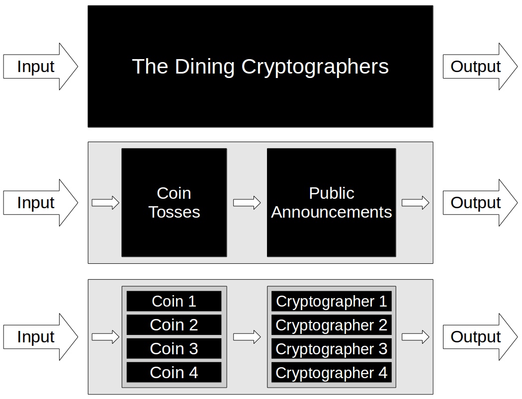
Refer to caption
Figure 1: Schematic representation of the Dining Cryptographers protocol as: (i) a monolithic channel (top); (ii) a composition of two channels (middle); and (ii) a composition of eight channels (bottom).

Despite the Dining Cryptographers relative simplicity, deriving its channel can be a challenging task. Since each of the nn cryptographers can announce either 00 or 11, the size of the output set 𝒴\mathcal{Y}, and, consequently, of the channel, increases exponentially with the number of cryptographers. The problem is worsened by the fact that computing the probabilities constituting the channel’s entries is not trivial. The algebra we introduce in this paper allows for an intuitive and compositional way of building a protocol’s channel from each of its components. To illustrate the concept, Figure 1 depicts three alternative representations, using channels, for the Dining Cryptographers with 44 cryptographers and 44 coins. In all models, the input is the identity of the payer (one of the cryptographers or the NSA), and the output are the public announcements of all cryptographers. The top model uses a single (enormous) channel to represent the protocol; the middle one models the protocol as the interaction between two smaller components (the coins and the party of cryptographers); the bottom one uses interactions between even smaller channels (one for each coin and each cryptographer).

The main contributions of this paper are the following.

  • •

    We formalize several common operators for channel composition used in the literature, each matching a typical interaction between system components. We prove several relevant algebraic and information-leakage properties of these operators.

  • •

    We show that the substitution of components in a system may be subject to unexpected, and perhaps counter-intuitive, results. In particular, we show that overall leakage may increase even when the new component is more secure than the one it is replacing (e.g., Theorems 5.5 and 5.6).

  • •

    We show how the proposed algebra can be used to simplify large system specifications in order to facilitate the computation of information leakage bounds, given in terms of the gg-leakage framework [1, 11, 12, 2].

  • •

    We demonstrate our results on the specification and analysis of the Crowds Protocol [13]. We use the proposed algebra to justify a new algorithm to compute leakage bounds for this protocol.

Detailed proofs of all of our technical results can be found in Appendix 0.A.

Plan of the paper.

The remainder of this paper is organized as follows. In Section 2 we review fundamental concepts from QIF. In Section 3 we introduce our channel operators, and in Section 4 we provide their algebraic properties. In Section 5 we present our main results, concerning information leakage in channel composition. In Section 6 we develop a detailed case study of the Crowds protocol. Finally, in Section 7 we discuss related work, and in Section 8 we conclude.

2 Preliminaries

In this section we review some fundamentals from quantitative information flow.

Secrets, gain functions and vulnerability.

A secret is some piece of sensitive information that one wants to protect from disclosure. Such sensitive information may concern, for instance, a user’s password, identity, personal data, or current location. We represent by 𝒳\mathcal{X} the set of possible secret values the secret may take.

The adversary is assumed to have, before observing the system’s behaviour, some a priori partial knowledge about the secret value. This knowledge is modeled as a probability distribution π∈𝔻​𝒳\pi\in\mathbb{D}\mathcal{X}, where 𝔻​𝒳\mathbb{D}\mathcal{X} denotes the set of all probability distributions on 𝒳\mathcal{X}. We call π\pi a prior distribution, or simply a prior.

To quantify how vulnerable a secret is—i.e., how prone it is to exploitation by the adversary— we employ a function that maps probability distributions to the real numbers (or, more in general, to any ordered set). Many functions have been used in the literature, such as Shannon entropy [15], guessing-entropy [16], Bayes vulnerability [17], and Rényi min-entropy [6]. Recently, the gg-leakage [1] framework was proposed, and it proved to be very successful in capturing a variety of different scenarios, including those in which the adversary benefits from guessing part of secret, guessing a secret approximately, guessing the secret within a number of tries, or gets punished for guessing wrongly. In particular, the framework has been shown to be able to capture all functions mentioned above [12]. In this framework, a finite set 𝒲\mathcal{W} of actions is available to the adversary, and a gain-function g:𝒲×𝒳→[0,1]g{:}\mathcal{W}{\times}\mathcal{X}{\rightarrow}[0,1] is used to describe the benefit g⁡(w,x)g(w,x) an adversary obtains when he performs action w∈𝒲w{\in}\mathcal{W}, and the secret value is x∈𝒳x{\in}\mathcal{X}. Given an appropriate gain-function gg, the secret’s (prior) gg-vulnerability is defined as the expected value of the adversary’s gain if he chooses a best possible action,

Vg​[π]=max⁡∑x∈𝒳w∈𝒲⁡π⁡(x)​g​(w,x),V_{g}[\pi]=\max\limits_{w\in\mathcal{W}}\sum_{x\in\mathcal{X}}\pi(x)g(w,x),

and the greater its value, the more vulnerable, or insecure, the secret is.

Channels and posterior vulnerabilities

In the QIF framework, a system is usually modeled as an (information theoretic) channel taking a secret input x∈𝒳x{\in}\mathcal{X}, and producing a public, or observable, output y∈𝒴y{\in}\mathcal{Y}. Each element of 𝒴\mathcal{Y} represents a behaviour from the system that can be discerned by the adversary. Formally, a channel is a function C:𝒳×𝒴→ℝC{:}\mathcal{X}{\times}\mathcal{Y}{\rightarrow}\mathbb{R} such that C⁡(x,y)C(x,y) is the conditional probability p⁡(y∣x)p(y{\mid}x) of the system producing output y∈𝒴y{\in}\mathcal{Y} when input is x∈𝒳x{\in}\mathcal{X}.

A channel CC together with a prior π\pi induce a joint probability distribution pp on the set 𝒳×𝒴\mathcal{X}{\times}\mathcal{Y}, given by p⁡(x,y)=π⁡(x)​C​(x,y)p(x,y)=\pi(x)C(x,y). From this joint distribution we can derive, for every x∈𝒳x{\in}\mathcal{X} and y∈𝒴y{\in}\mathcal{Y}, the marginal probabilities p⁡(x)=∑yp⁡(x,y)p(x)=\sum_{y}p(x,y) and p⁡(y)=∑xp⁡(x,y)p(y)=\sum_{x}p(x,y), and the conditional probabilities p⁡(x∣y)=p⁡(x,y)/p⁡(y)p(x{\mid}y)=\nicefrac{{p(x,y)}}{{p(y)}} and p⁡(y∣x)=p⁡(x,y)/p⁡(x)p(y{\mid}x)=\nicefrac{{p(x,y)}}{{p(x)}}. Note that p⁡(x)=π⁡(x)p(x)=\pi(x) and, if p⁡(x)≠0p(x)\neq 0, p⁡(y∣x)=C⁡(x,y)p(y{\mid}x)=C(x,y).

By observing the output produced by the system, the adversary can update his knowledge about the secret value. More specifically, if the system outputs y∈𝒴y{\in}\mathcal{Y}, an adversary can update the prior π\pi to a revised posterior distribution pX|y∈𝔻​𝒳p_{X{\mid}y}\in\mathbb{D}\mathcal{X} on 𝒳\mathcal{X} given yy, defined for all x∈𝒳x{\in}\mathcal{X} and y∈𝒴y{\in}\mathcal{Y} as pX|y​(x)=p​(x∣y)p_{X{\mid}y}(x)=p(x{\mid}y).

Example 1

Let 𝒳={x1,x2,x3}\mathcal{X}=\{x_{1},x_{2},x_{3}\} and 𝒴={y1,y2,y3,y4}\mathcal{Y}=\{y_{1},y_{2},y_{3},y_{4}\} be input and output sets. Let π=(1/2,1/3,1/6)\pi=(\nicefrac{{1}}{{2}},\nicefrac{{1}}{{3}},\nicefrac{{1}}{{6}}) be a prior, and CC be the channel below. The combination of π\pi and CC yield a joint probability pp, according to the tables below.

Cy1y2y3y4x11/62/31/60x21/21/41/40x31/21/301/6⟶πpy1y2y3y4x11/121/31/120x21/61/121/120x31/121/1801/36\displaystyle\begin{array}[]{|c|cccc|}\hline\cr C&\,\,\,y_{1}&\,\,\,y_{2}&\,\,\,y_{3}&\,\,\,y_{4}\\ \hline\cr x_{1}&\nicefrac{{1}}{{6}}&\nicefrac{{2}}{{3}}&\nicefrac{{1}}{{6}}&0\\ x_{2}&\nicefrac{{1}}{{2}}&\nicefrac{{1}}{{4}}&\nicefrac{{1}}{{4}}&0\\ x_{3}&\nicefrac{{1}}{{2}}&\nicefrac{{1}}{{3}}&0&\nicefrac{{1}}{{6}}\\ \hline\cr\end{array}\quad\stackrel{{\scriptstyle\pi}}{{\longrightarrow}}\quad\begin{array}[]{|c|cccc|}\hline\cr p&\,\,\,y_{1}&\,\,\,y_{2}&\,\,\,y_{3}&\,\,\,y_{4}\\ \hline\cr x_{1}&\nicefrac{{1}}{{12}}&\nicefrac{{1}}{{3}}&\nicefrac{{1}}{{12}}&0\\ x_{2}&\nicefrac{{1}}{{6}}&\nicefrac{{1}}{{12}}&\nicefrac{{1}}{{12}}&0\\ x_{3}&\nicefrac{{1}}{{12}}&\nicefrac{{1}}{{18}}&0&\nicefrac{{1}}{{36}}\\ \hline\cr\end{array}

By summing the columns of the second table, we obtain the marginal probabilities p⁡(y1)=1/3p(y_{1}){=}\nicefrac{{1}}{{3}}, p⁡(y2)=17/36p(y_{2}){=}\nicefrac{{17}}{{36}}, p⁡(y3)=1/6p(y_{3}){=}\nicefrac{{1}}{{6}} and p⁡(y4)=1/36p(y_{4}){=}\nicefrac{{1}}{{36}}. These marginal probabilities yield the posterior distributions pX|y1=(1/4,1/2,1/4)p_{X\mid y_{1}}{=}(\nicefrac{{1}}{{4}},\nicefrac{{1}}{{2}},\nicefrac{{1}}{{4}}), pX|y2=(12/17,3/17,2/17)p_{X\mid y_{2}}{=}(\nicefrac{{12}}{{17}},\nicefrac{{3}}{{17}},\nicefrac{{2}}{{17}}), pX|y3=(1/2,1/2,0)p_{X\mid y_{3}}{=}(\nicefrac{{1}}{{2}},\nicefrac{{1}}{{2}},0), and pX|y4=(0,0,1)p_{X\mid y_{4}}{=}(0,0,1). ∎

The posterior gg-vulnerability of a prior π\pi and a channel CC is defined as the expected value of the secret’s gg-vulnerability after the execution of the system:

Vg[π⟩C]=∑y∈𝒴maxw∈𝒲∑x∈𝒳C(x,y)π(x)g(x,w).V_{g}[\pi\,\rangle\,C]=\sum_{y\in\mathcal{Y}}\max\limits_{w\in\mathcal{W}}\sum_{x\in\mathcal{X}}C(x,y)\pi(x)g(x,w).

The information leakage of a prior and a channel is a measure of the increase in secret vulnerability caused by the observation of the system’s output. Leakage is, thus, defined as a comparison between the secret’s prior and posterior vulnerabilities. Formally, for a gain-function gg, and given prior π\pi and channel CC, the multiplicative and the additive versions of gg-leakage are defined, respectively, as

ℒg[π⟩C]=Vg[π⟩C]/Vg​[π],andℒg+[π⟩C]=Vg[π⟩C]−Vg[π].\mathcal{L}_{g}[\pi\,\rangle\,C]=\nicefrac{{V_{g}[\pi\,\rangle\,C]}}{{V_{g}[\pi]}},\qquad\text{and}\qquad\mathcal{L}_{g}^{+}[\pi\,\rangle\,C]=V_{g}[\pi\,\rangle\,C]-V_{g}[\pi].

Since prior vulnerability does not depend on the channel, we have that

ℒg[π⟩C1]≥ℒg[π⟩C2]⇔ℒg+[π⟩C1]≥ℒg+[π⟩C2]⇔Vg[π⟩C1]≥Vg[π⟩C2],\displaystyle\mathcal{L}_{g}[\pi\,\rangle\,C_{1}]\geq\mathcal{L}_{g}[\pi\,\rangle\,C_{2}]\,\,\Leftrightarrow\,\,\mathcal{L}_{g}^{+}[\pi\,\rangle\,C_{1}]\geq\mathcal{L}_{g}^{+}[\pi\,\rangle\,C_{2}]\,\,\Leftrightarrow\,\,V_{g}[\pi\,\rangle\,C_{1}]\geq V_{g}[\pi\,\rangle\,C_{2}],

and, hence, the posterior vulnerability of a channel is greater than that of another if, and only if, both multiplicative and additive leakage also are.

Channel Ordering and the Coriaceous Theorem.

We now define a common composition of channels, called cascading. This operation can be interpreted as the result of a channel post-processing the output of another channel. Formally, given two channels C:𝒳×𝒴→ℝC{:}\mathcal{X}{\times}\mathcal{Y}{\rightarrow}\mathbb{R} and D:𝒴×𝒵→ℝD{:}\mathcal{Y}{\times}\mathcal{Z}{\rightarrow}\mathbb{R}, their cascading is defined as

(C​D)​(x,z)=∑y∈𝒴C⁡(x,y)​D​(y,z),(CD)(x,z)=\sum_{y\in\mathcal{Y}}C(x,y)D(y,z),

for all x∈𝒳x{\in}\mathcal{X} and z∈𝒵z{\in}\mathcal{Z}. If we represent channels as tables, as we did in Example 1, the cascading operation corresponds to a simple matrix multiplication.

An important question in QIF is to decide whether a channel C2C_{2} is always at least as secure as a channel C1C_{1}, meaning that C2C_{2} never leaks more information than C1C_{1}, for whatever choice of gain function gg and of prior π\pi. Let us write C1⊑∘C2C_{1}\sqsubseteq_{\circ}C_{2} (read as C2C_{2} refines C1C_{1}) to denote that there exists a channel DD such that C1​D=C2C_{1}D=C_{2}. We write C1≈C2C_{1}\approx C_{2}, and say that C1C_{1} is equivalent to C2C_{2}, when both C1⊑∘C2C_{1}\sqsubseteq_{\circ}C_{2} and C2⊑∘C1C_{2}\sqsubseteq_{\circ}C_{1} hold. The Coriaceous Theorem [1, 2] states that, C1⊑∘C2C_{1}\sqsubseteq_{\circ}C_{2} if, and only if, Vg[π⟩C1]≥Vg[π⟩C2]V_{g}[\pi\,\rangle\,C_{1}]\geq V_{g}[\pi\,\rangle\,C_{2}] for all π\pi, gg. This result reduces the comparison of channel security to a simple algebraic test.

The refinement relation ⊑∘\sqsubseteq_{\circ} is a preorder on the set of all channels having the same input set. This preorder can be made into a partial order by using abstract channels [2], an equivalence relation that equates all channels presenting same leakage for all priors and gain functions. This partial order coincides with how much information channels leak, being the least secure channel (i.e., the “most leaky” one) at its bottom, and the most secure (i.e., the “least leaky”) at its top.

3 Operators on channel composition

We shall say that two channels are compatible if they have the same input set. Given a set 𝒳\mathcal{X}, we denote by 𝒞𝒳\mathcal{C}_{\mathcal{X}} the set of all channels that have 𝒳\mathcal{X} as input set. Two compatible channels with same output set are said to be of the same type.

In this section we introduce several binary operators—i.e., functions of type (𝒞𝒳×𝒞𝒳)→𝒞𝒳(\mathcal{C}_{\mathcal{X}}{\times}\mathcal{C}_{\mathcal{X}}){\rightarrow}\mathcal{C}_{\mathcal{X}}—matching typical interactions between system components, and prove relevant algebraic properties of these operators. We refer to the result of an operator as a compound system, and we refer to its arguments as components.

3.1 The parallel composition operator ∥\parallel

The parallel composition operator ∥\parallel models the composition of two independent channels in which the same input is fed to both of them, and their outputs are then observed. By independent, we mean that the output of one channel does not interfere with that of the other. This assumption, while not universal, captures a great variety of real-world scenarios, and is, hence, of practical interest.

For example, side-channel attacks occur when the adversary combines his observation of the system’s output with some alternative way of inferring information about the secret (e.g., by observing physical properties of the system execution, such as time elapsed [18, 19] or change in magnetic fields [20]). In such attacks, the channel used by the adversary to infer information about the secret can be modeled as the composition of a channel representing the program’s intended behaviour in parallel with a channel modeling the relation between the secret and the physical properties of the hardware.

Definition 1 (Parallel composition operator ∥\parallel)

Given compatible channels C1:𝒳×𝒴1→ℝC_{1}{:}\mathcal{X}{\times}\mathcal{Y}_{1}{\rightarrow}\mathbb{R} and C2:𝒳×𝒴2→ℝC_{2}{:}\mathcal{X}{\times}\mathcal{Y}_{2}{\rightarrow}\mathbb{R}, their parallel composition C1|C2:𝒳×(𝒴1×𝒴2)→ℝC_{1}\parallel C_{2}:\mathcal{X}{\times}(\mathcal{Y}_{1}{\times}\mathcal{Y}_{2}){\rightarrow}\mathbb{R} is defined as, for all x∈𝒳x{\in}\mathcal{X}, y1∈𝒴1y_{1}{\in}\mathcal{Y}_{1}, and y2∈𝒴2y_{2}{\in}\mathcal{Y}_{2},

(C1∥C2)(x,(y1,y2))=C1(x,y1)C2(x,y2).(C_{1}\parallel C_{2})(x,(y_{1},y_{2}))=C_{1}(x,y_{1})C_{2}(x,y_{2}).

Notice that this definition comes from the independence property, as we have C1​(x,y1)​C2​(x,y2)=p⁡(y1∣x)​p​(y2∣x)=p⁡(y1,y2∣x)C_{1}(x,y_{1})C_{2}(x,y_{2})=p(y_{1}{\mid}x)p(y_{2}{\mid}x)=p(y_{1},y_{2}{\mid}x).

3.2 The visible choice operator p⋅Γ⊔{}_{\mathit{p}}{\mathbin{\mathaccent 0{\cdot}\sqcup}}

The visible choice operator p⋅Γ⊔{}_{\mathit{p}}{\mathbin{\mathaccent 0{\cdot}\sqcup}} models a scenario in which the system has a choice among two different components to process the secret it was fed as input. With probability pp, the system feeds the secret to the first component, and, with probability 1−p1{-}p, it feeds the secret to the second component. In the end, the system reveals the output produced, together with the identification of which component was used (whence, the name “visible choice”).

As an example, consider an adversary trying to gain information about a secret processed by a website. The adversary knows that the website has two servers, one of which will be assigned to answer the request according to a known probability distribution. Suppose, furthermore, that the adversary can identify which server was used by measuring its response time to the request. This adversary’s view of the system can be modeled as the visible choice between the two servers, since, although the adversary does not know in advance which server will be used, he learns it when he gets the output from the system.

Before formalizing this operator, we need to define the disjoint union of sets. Given any sets 𝒜\mathcal{A} and ℬ\mathcal{B}, their disjoint union is 𝒜⊔ℬ=(𝒜×{1})∪(ℬ×{2})\mathcal{A}\sqcup\mathcal{B}=(\mathcal{A}\times\{1\})\cup(\mathcal{B}\times\{2\}).

Definition 2 (Visible choice operator p⋅Γ⊔{}_{\mathit{p}}{\mathbin{\mathaccent 0{\cdot}\sqcup}})

Given compatible channels C1:𝒳×𝒴1→ℝC_{1}:\mathcal{X}{\times}\mathcal{Y}_{1}{\rightarrow}\mathbb{R} and C2:𝒳×𝒴2→ℝC_{2}{:}\mathcal{X}{\times}\mathcal{Y}_{2}{\rightarrow}\mathbb{R}, their visible choice is the channel C1⋅Γ⊔pC2:𝒳×(𝒴1⊔𝒴2)→ℝC_{1}\;{{}_{\mathit{p}}{\mathbin{\mathaccent 0{\cdot}\sqcup}}}\;C_{2}:\mathcal{X}{\times}(\mathcal{Y}_{1}\sqcup\mathcal{Y}_{2}){\rightarrow}\mathbb{R} defined as, for all x∈𝒳x{\in}\mathcal{X} and (y,i)∈𝒴1⊔𝒴2(y,i)\in\mathcal{Y}_{1}\sqcup\mathcal{Y}_{2},

(C1⋅Γ⊔pC2)(x,(y,i))={p​C1​(x,y),if ​i=1,(1−p)​C2​(x,y),if ​i=2.(C_{1}\;{{}_{\mathit{p}}{\mathbin{\mathaccent 0{\cdot}\sqcup}}}\;C_{2})(x,(y,i))=\begin{cases}pC_{1}(x,y),&\mbox{if }i=1,\\ (1{-}p)C_{2}(x,y),&\mbox{if }i=2.\end{cases}

3.3 The hidden choice operator p⊕{}_{\mathit{p}}{\oplus}

Similarly to the visible choice case, the hidden choice operator p⊕{}_{\mathit{p}}{\oplus} models a scenario in which the system has a choice of feeding its secret input to one component (with probability pp), or to another component (with probability 1−p1{-}p). In the end, the system reveals the output produced, but, unlike the visible choice case, the component which was used is not revealed. Hence, when the same observations are randomized between the two channels, the adversary cannot identify which channel produced the observation (whence, the name “hidden choice”).

As an example, consider statistical surveys that ask some sensitive yes/no question, such as whether the respondent has made use of any illegal substances. To encourage individuals to participate on the survey, it is necessary to control leakage of their sensitive information, while preserving the accuracy of statistical information in the ensemble of their answers. A common protocol to achieve this goal works as follows [21]. Each respondent throws a coin, without letting the questioner know the corresponding result. If the result is heads, the respondent answers the question honestly, and if the result is tails, he gives a random response (obtained, for example, according to the result of a second coin toss). If the coins are fair, this protocol can be modeled as the hidden choice T1/2⊕CT{\;{{}_{\mathit{\nicefrac{{1}}{{2}}}}{\oplus}}\;}C between a channel TT representing an honest response (revealing the secret completely), and a channel CC representing a random response (revealing nothing about the secret). The protocol is, hence, a channel that masks the result of TT.

Definition 3 (Hidden choice operator p⊕{}_{\mathit{p}}{\oplus})

Given compatible channels C1:𝒳×𝒴1→ℝC_{1}:\mathcal{X}{\times}\mathcal{Y}_{1}{\rightarrow}\mathbb{R} and C2:𝒳×𝒴2→ℝC_{2}{:}\mathcal{X}{\times}\mathcal{Y}_{2}{\rightarrow}\mathbb{R}, their hidden choice is the channel C1⊕pC2:𝒳×(𝒴1∪𝒴2)→ℝC_{1}\;{{}_{\mathit{p}}{\oplus}}\;C_{2}:\mathcal{X}{\times}(\mathcal{Y}_{1}\cup\mathcal{Y}_{2}){\rightarrow}\mathbb{R} defined as, for all x∈𝒳x{\in}\mathcal{X} and y∈𝒴1∪𝒴2y{\in}\mathcal{Y}_{1}\cup\mathcal{Y}_{2},

(C1⊕pC2)(x,y)={p​C1​(x,y)+(1−p)​C2​(x,y),if ​y∈𝒴1∩𝒴2,p​C1​(x,y),if ​y∈𝒴1∖𝒴2,(1−p)​C2​(x,y),if ​y∈𝒴2∖𝒴1.(C_{1}\;{{}_{\mathit{p}}{\oplus}}\;C_{2})(x,y)=\begin{cases}pC_{1}(x,y)+(1{-}p)C_{2}(x,y),&\mbox{if }y\in\mathcal{Y}_{1}\cap\mathcal{Y}_{2},\\ pC_{1}(x,y),&\mbox{if }y\in\mathcal{Y}_{1}\setminus\mathcal{Y}_{2},\\ (1{-}p)C_{2}(x,y),&\mbox{if }y\in\mathcal{Y}_{2}\setminus\mathcal{Y}_{1}.\end{cases}

Note that when the output sets of C1C_{1} and C2C_{2} are disjoint the adversary can always identify the channel used, and we have C1p⋅Γ⊔C2≈C1p⊕C2C_{1}{\;{{}_{\mathit{p}}{\mathbin{\mathaccent 0{\cdot}\sqcup}}}\;}C_{2}{\approx}C_{1}{\;{{}_{\mathit{p}}{\oplus}}\;}C_{2}.

3.4 A compositional description of the Dining Cryptographers

We now revisit the Dining Cryptographers protocol example from Section 1, showing how it can be modeled using our composition operators.

We consider that there are 44 cryptographers and 44 coins, and denote the protocol’s channel by 𝐷𝑖𝑛𝑖𝑛𝑔\mathit{Dining}. The channel’s input set is 𝒳={c1,c2,c3,c4,n}\mathcal{X}=\{c_{1},c_{2},c_{3},c_{4},n\}, in which cic_{i} represents that cryptographer ii is the payer, and nn represents that the NSA is the payer. The channel’s output set is 𝒴={0,1}4\mathcal{Y}=\{0,1\}^{4}, i.e., all 44-tuples representing possible announcements by all cryptographers, in order.

Following the scheme in Figure 1 (middle), we begin by modeling the protocol as the interaction between two channels, 𝐶𝑜𝑖𝑛𝑠\mathit{Coins} and 𝐴𝑛𝑛𝑜𝑢𝑛𝑐𝑒𝑚𝑒𝑛𝑡𝑠\mathit{Announcements}, representing, respectively, the coin tosses and the cryptographers’ public announcements. Since in the protocol first the coins are tossed, and only then the corresponding results are passed on to the party of cryptographers, 𝐷𝑖𝑛𝑖𝑛𝑔\mathit{Dining} can be described as the cascading of these two channels:

𝐷𝑖𝑛𝑖𝑛𝑔=(𝐶𝑜𝑖𝑛𝑠)​(𝐴𝑛𝑛𝑜𝑢𝑛𝑐𝑒𝑚𝑒𝑛𝑡𝑠).\mathit{Dining}=(\mathit{Coins})(\mathit{Announcements}).
 𝐶𝑜𝑖𝑛i\mathit{Coin}_{i}   Tails   Heads
c1c_{1} pip_{i} 1−pi1{-}p_{i}
c2c_{2} pip_{i} 1−pi1{-}p_{i}
c3c_{3} pip_{i} 1−pi1{-}p_{i}
c4c_{4} pip_{i} 1−pi1{-}p_{i}
nn pip_{i} 1−pi1{-}p_{i}
Table 1: Channel representing toss of coin 𝐶𝑜𝑖𝑛i\mathit{Coin}_{i}.

To specify channel 𝐶𝑜𝑖𝑛𝑠\mathit{Coins}, we use the parallel composition of channels 𝐶𝑜𝑖𝑛1\mathit{Coin}_{1}, 𝐶𝑜𝑖𝑛2\mathit{Coin}_{2}, 𝐶𝑜𝑖𝑛3\mathit{Coin}_{3} and 𝐶𝑜𝑖𝑛4\mathit{Coin}_{4}, each representing one coin toss. Letting pip_{i} denote the probability of coin ii landing on tails, these channels are defined as on Table 1.

Besides the result of the tosses, 𝐶𝑜𝑖𝑛𝑠\mathit{Coins} also needs to pass on to 𝐴𝑛𝑛𝑜𝑢𝑛𝑐𝑒𝑚𝑒𝑛𝑡𝑠\mathit{Announcements} the identity of the payer. We then introduce a fifth channel, I:𝒳×𝒳→ℝI{:}\mathcal{X}{\times}\mathcal{X}{\rightarrow}\mathbb{R}, that simply outputs the secret, i.e., I⁡(x1,x2)=1I(x_{1},x_{2})=1 if x1=x2x_{1}=x_{2}, and 00 otherwise. Hence, a complete definition of channel 𝐶𝑜𝑖𝑛𝑠\mathit{Coins} is

𝐶𝑜𝑖𝑛𝑠=𝐶𝑜𝑖𝑛1|𝐶𝑜𝑖𝑛2|𝐶𝑜𝑖𝑛3|𝐶𝑜𝑖𝑛4|I.\mathit{Coins}=\mathit{Coin}_{1}\parallel\mathit{Coin}_{2}\parallel\mathit{Coin}_{3}\parallel\mathit{Coin}_{4}\parallel I.

As we will show in Section 4, parallel composition is associative, allowing us to omit parentheses in the equation above.

We now specify the channel 𝐴𝑛𝑛𝑜𝑢𝑛𝑐𝑒𝑚𝑒𝑛𝑡𝑠\mathit{Announcements}, which takes as input a 55-tuple with five terms whose first four elements are the results of the coin tosses, and the fifth is the identity of the payer. For that end, we describe each cryptographer as a channel with this 55-tuple as input, and with the set of possible announcements {0,1}\{0,1\} as output set. 𝐶𝑟𝑦𝑝𝑡𝑜1\mathit{Crypto}_{1} below describes the first cryptographer.

𝐶𝑟𝑦𝑝𝑡𝑜1​(t1,t2,t3,t4,x)={1​, if ​t4=t1​ and ​x=c1​, or ​t4≠t1​ and ​x≠c10​, otherwise\mathit{Crypto}_{1}(t_{1},t_{2},t_{3},t_{4},x)=\begin{cases}1\mbox{, if }t_{4}=t_{1}\mbox{ and }x=c_{1}\mbox{, or }t_{4}\neq t_{1}\mbox{ and }x\neq c_{1}\\ 0\mbox{, otherwise}\end{cases}

Channels 𝐶𝑟𝑦𝑝𝑡𝑜2\mathit{Crypto}_{2}, 𝐶𝑟𝑦𝑝𝑡​o3\mathit{Crypt}o_{3} and 𝐶𝑟𝑦𝑝𝑡𝑜4\mathit{Crypto}_{4} describing the remaining cryptographers are defined analogously. Channel 𝐴𝑛𝑛𝑜𝑢𝑛𝑐𝑒𝑚𝑒𝑛𝑡𝑠\mathit{Announcements} is, hence, defined as

𝐴𝑛𝑛𝑜𝑢𝑛𝑐𝑒𝑚𝑒𝑛𝑡𝑠=𝐶𝑟𝑦𝑝𝑡𝑜1|𝐶𝑟𝑦𝑝𝑡𝑜2|𝐶𝑟𝑦𝑝𝑡𝑜3|𝐶𝑟𝑦𝑝𝑡𝑜4.\mathit{Announcements}=\mathit{Crypto}_{1}\parallel\mathit{Crypto}_{2}\parallel\mathit{Crypto}_{3}\parallel\mathit{Crypto}_{4}.

Note that our operators allow for an intuitive and succinct representation of the channel 𝐷𝑖𝑛𝑖𝑛𝑔\mathit{Dining} modeling the Dining Cryptographers protocol, even when the number of cryptographers and coins is large. Moreover, the channel is easy to compute: we need only to first calculate the parallel compositions within channels 𝐶𝑟𝑦𝑝𝑡𝑜\mathit{Crypto} and 𝐴𝑛𝑛𝑜𝑢𝑛𝑐𝑒𝑚𝑒𝑛𝑡𝑠\mathit{Announcements}, and then multiply these channels’ matrices.

4 Algebraic properties of channel operators

In this section we prove a series of relevant algebraic properties of our channel operators. These properties are the key for building channels in a compositional way, and, more importantly, for deriving information flow properties of a compound system in terms of those of its components.

We begin by defining a notion of equivalence stricter than ≈\approx, which equates any two channels that are identical modulo a permutation of their columns.

Definition 4 (Channel equality)

Let C1:𝒳×𝒴1→ℝC_{1}:\mathcal{X}{\times}\mathcal{Y}_{1}{\rightarrow}\mathbb{R} and C2:𝒳×𝒴2→ℝC_{2}:\mathcal{X}{\times}\mathcal{Y}_{2}{\rightarrow}\mathbb{R} be compatible channels. We say that C1C_{1} and C2C_{2} are equal up to a permutation , and write C1​=∘​C2C_{1}{\;\overset{\circ}{=}\;}C_{2}, if there is a bijection ψ:𝒴1→𝒴2\psi{:}\mathcal{Y}_{1}{\rightarrow}\mathcal{Y}_{2} such that C1​(x,y)=C2​(x,ψ⁡(y))C_{1}(x,y){=}C_{2}(x,\psi(y)) for all x∈𝒳x{\in}\mathcal{X}, y∈𝒴1y{\in}\mathcal{Y}_{1}.

Note that, if C1​=∘​C2C_{1}{\;\overset{\circ}{=}\;}C_{2}, then C1≈C2C_{1}{\approx}C_{2}. 11 1 A complete, formal definition of such bijections can be found in Appendix 0.A.

In remaining of this section, let C1:𝒳×𝒴1→ℝC_{1}:\mathcal{X}{\times}\mathcal{Y}_{1}{\rightarrow}\mathbb{R}, C2:𝒳×𝒴2→ℝC_{2}:\mathcal{X}{\times}\mathcal{Y}_{2}{\rightarrow}\mathbb{R} and C3:𝒳×𝒴3→ℝC_{3}:\mathcal{X}{\times}\mathcal{Y}_{3}{\rightarrow}\mathbb{R} be compatible channels, and p,q∈[0,1]p,q\in[0,1] be probability values.

4.1 Properties regarding channel operators

We first establish our operators’ associativity and commutativity properties.

Proposition 1 (Commutative Properties)
C1∥C2=∘C2∥C1,C1p⋅Γ⊔C2=∘C2(1−p)⋅Γ⊔C1,andC1p⊕C2=C2(1−p)⊕C1.C_{1}{\parallel}C_{2}{\;\overset{\circ}{=}\;}C_{2}{\parallel}C_{1},\quad C_{1}{\;{{}_{\mathit{p}}{\mathbin{\mathaccent 0{\cdot}\sqcup}}}\;}C_{2}{\;\overset{\circ}{=}\;}C_{2}{\;{{}_{\mathit{(1-p)}}{\mathbin{\mathaccent 0{\cdot}\sqcup}}}\;}C_{1},\,\,\text{and}\,\,\,\,C_{1}{\;{{}_{\mathit{p}}{\oplus}}\;}C_{2}=C_{2}{\;{{}_{\mathit{(1-p)}}{\oplus}}\;}C_{1}.
Proposition 2 (Associative Properties)
(C1∥C2)∥C3=∘C1∥(C2∥C3),(C1p⋅Γ⊔C2)q⋅Γ⊔C3=∘C1p′⋅Γ⊔(C2q′⋅Γ⊔C3),\begin{array}[]{cc}(C_{1}\parallel C_{2})\parallel C_{3}{\;\overset{\circ}{=}\;}C_{1}\parallel(C_{2}\parallel C_{3}),&\,\,\,\,\,(C_{1}\;{{}_{\mathit{p}}{\mathbin{\mathaccent 0{\cdot}\sqcup}}}\;C_{2})\;{{}_{\mathit{q}}{\mathbin{\mathaccent 0{\cdot}\sqcup}}}\;C_{3}{\;\overset{\circ}{=}\;}C_{1}\;{{}_{\mathit{p^{\prime}}}{\mathbin{\mathaccent 0{\cdot}\sqcup}}}\;(C_{2}\;{{}_{\mathit{q^{\prime}}}{\mathbin{\mathaccent 0{\cdot}\sqcup}}}\;C_{3}),\end{array}
and (C1p⊕C2)q⊕C3=C1p′⊕(C2q′⊕C3),​ s.t. p′=p​q and q′=(q−p​q)/(1−p​q).\begin{array}[]{cc}\text{and }&(C_{1}{\;{{}_{\mathit{p}}{\oplus}}\;}C_{2}){\;{{}_{\mathit{q}}{\oplus}}\;}C_{3}=C_{1}{\;{{}_{\mathit{p^{\prime}}}{\oplus}}\;}(C_{2}{\;{{}_{\mathit{q^{\prime}}}{\oplus}}\;}C_{3}),\end{array}\text{ s.t. $p^{\prime}{=}pq$ and $q^{\prime}{=}\nicefrac{{(q-pq)}}{{(1-pq)}}$.}

We now turn our attention to two kinds of channels that will be recurrent building blocks for more complex channels. A null channel is any channel 0¯:𝒳×𝒴→ℝ\overline{0}:\mathcal{X}{\times}\mathcal{Y}{\rightarrow}\mathbb{R} such that, for every prior π\pi and gain-function gg, Vg[π⟩0¯]=Vg[π]V_{g}[\pi\,\rangle\,\overline{0}]=V_{g}[\pi]. That is, a null channel never leaks any information. A channel 0¯\overline{0} is null if, and only if, 0¯​(x,y)=0¯​(x′,y)\overline{0}(x,y)=\overline{0}(x^{\prime},y) for all y∈𝒴y{\in}\mathcal{Y} and x,x′∈𝒳x,x^{\prime}{\in}\mathcal{X}. On the other hand, a transparent channel is any channel I¯:𝒳×𝒴→ℝ\overline{I}:\mathcal{X}{\times}\mathcal{Y}{\rightarrow}\mathbb{R} that leaks at least as much information as any other compatible channel, for every prior and gain-function. A channel I¯\overline{I} is transparent if, and only if, for each y∈𝒴y{\in}\mathcal{Y}, there is at most one x∈𝒳x{\in}\mathcal{X} such that I¯​(x,y)>0\overline{I}(x,y){>}0. The following properties hold for any null channel 0¯\overline{0} and transparent channel I¯\overline{I} compatible with C1C_{1}, C2C_{2} and C3C_{3}.

Proposition 3 (Null and Transparent Channel Properties)
null channel:(C1∥0¯)≈C1,C1⊑∘(C1p⋅Γ⊔0¯),C1⊑∘(C1p⊕0¯).transparent channel:(C1∥I¯)≈I¯,(C1p⋅Γ⊔I¯)⊑∘C1.\begin{array}[]{rlll}\text{null channel:}&(C_{1}\parallel\overline{0})\approx C_{1},&C_{1}\sqsubseteq_{\circ}(C_{1}\;{{}_{\mathit{p}}{\mathbin{\mathaccent 0{\cdot}\sqcup}}}\;\overline{0}),&C_{1}\sqsubseteq_{\circ}(C_{1}\;{{}_{\mathit{p}}{\oplus}}\;\overline{0}).\\[5.69054pt] \text{transparent channel:}&(C_{1}\parallel\overline{I})\approx\overline{I},&(C_{1}\;{{}_{\mathit{p}}{\mathbin{\mathaccent 0{\cdot}\sqcup}}}\;\overline{I})\sqsubseteq_{\circ}C_{1}.&\end{array}

Note that, in general, (C1⊕pI¯)⋢∘C1(C_{1}\;{{}_{\mathit{p}}{\oplus}}\;\overline{I})\not\sqsubseteq_{\circ}C_{1}. To see why, consider the two transparent channels I¯1\overline{I}_{1} and I¯2\overline{I}_{2}, with both input and output sets equal {1,2}\{1,2\}, given by I¯1​(x,x′)=1\overline{I}_{1}(x,x^{\prime})=1 if x=x′x{=}x^{\prime}, and 00 otherwise, and I¯2​(x,x′)=0\overline{I}_{2}(x,x^{\prime})=0 if x=x′x{=}x^{\prime}, and 11 otherwise Then, I¯1p⊕I¯2\overline{I}_{1}\;{{}_{\mathit{p}}{\oplus}}\;\overline{I}_{2} is a null channel, and the property does not hold for C1=I¯1C_{1}=\overline{I}_{1}, I¯=I¯2\overline{I}=\overline{I}_{2}.

We now consider idemptotency.

Proposition 4 (Idempotency)
C1∥C1⊑∘C1,C1p⋅Γ⊔C1≈C1,andC1p⊕C1=C1.C_{1}\parallel C_{1}\sqsubseteq_{\circ}C_{1},\qquad C_{1}\;{{}_{\mathit{p}}{\mathbin{\mathaccent 0{\cdot}\sqcup}}}\;C_{1}\approx C_{1},\qquad\text{and}\qquad C_{1}\;{{}_{\mathit{p}}{\oplus}}\;C_{1}=C_{1}.

Note that C1|C1≈C1C_{1}{\parallel}C_{1}{\approx}C_{1} holds only when C1C_{1} is deterministic or equivalent to a deterministic channel.

Finally, we consider distributive properties. In particular, we explore interesting properties when an operator is “distributed” over itself.

Proposition 5 (Distribution over the same operator)
(C1∥C2)∥(C1∥C3)\displaystyle(C_{1}\parallel C_{2})\parallel(C_{1}\parallel C_{3}) ⊑∘C1∥(C2∥C3),\displaystyle\sqsubseteq_{\circ}C_{1}\parallel(C_{2}\parallel C_{3}),
C1⋅Γ⊔p(C2⋅Γ⊔qC3)\displaystyle C_{1}\;{{}_{\mathit{p}}{\mathbin{\mathaccent 0{\cdot}\sqcup}}}\;(C_{2}\;{{}_{\mathit{q}}{\mathbin{\mathaccent 0{\cdot}\sqcup}}}\;C_{3}) ≈(C1⋅Γ⊔pC2)⋅Γ⊔q(C1⋅Γ⊔pC3),\displaystyle\approx(C_{1}\;{{}_{\mathit{p}}{\mathbin{\mathaccent 0{\cdot}\sqcup}}}\;C_{2})\;{{}_{\mathit{q}}{\mathbin{\mathaccent 0{\cdot}\sqcup}}}\;(C_{1}\;{{}_{\mathit{p}}{\mathbin{\mathaccent 0{\cdot}\sqcup}}}\;C_{3}),
C1⊕p(C2⊕qC3)\displaystyle C_{1}\;{{}_{\mathit{p}}{\oplus}}\;(C_{2}\;{{}_{\mathit{q}}{\oplus}}\;C_{3}) =(C1⊕pC2)⊕q(C1⊕pC3).\displaystyle=(C_{1}\;{{}_{\mathit{p}}{\oplus}}\;C_{2})\;{{}_{\mathit{q}}{\oplus}}\;(C_{1}\;{{}_{\mathit{p}}{\oplus}}\;C_{3}).
Proposition 6 (Distribution over different operators)
C1∥(C2⋅Γ⊔pC3)\displaystyle C_{1}\parallel(C_{2}\;{{}_{\mathit{p}}{\mathbin{\mathaccent 0{\cdot}\sqcup}}}\;C_{3}) =∘(C1∥C2)⋅Γ⊔p(C1∥C3),\displaystyle{\;\overset{\circ}{=}\;}(C_{1}\parallel C_{2})\;{{}_{\mathit{p}}{\mathbin{\mathaccent 0{\cdot}\sqcup}}}\;(C_{1}\parallel C_{3}),
C1∥(C2⊕pC3)\displaystyle C_{1}\parallel(C_{2}\;{{}_{\mathit{p}}{\oplus}}\;C_{3}) =(C1∥C2)⊕p(C1∥C3),\displaystyle=(C_{1}\parallel C_{2})\;{{}_{\mathit{p}}{\oplus}}\;(C_{1}\parallel C_{3}),
C1⋅Γ⊔p(C2⊕qC3)\displaystyle C_{1}\;{{}_{\mathit{p}}{\mathbin{\mathaccent 0{\cdot}\sqcup}}}\;(C_{2}\;{{}_{\mathit{q}}{\oplus}}\;C_{3}) =(C1⋅Γ⊔pC2)⊕q(C1⋅Γ⊔pC3).\displaystyle=(C_{1}\;{{}_{\mathit{p}}{\mathbin{\mathaccent 0{\cdot}\sqcup}}}\;C_{2})\;{{}_{\mathit{q}}{\oplus}}\;(C_{1}\;{{}_{\mathit{p}}{\mathbin{\mathaccent 0{\cdot}\sqcup}}}\;C_{3}).

Unfortunately, the distribution of p⋅Γ⊔{}_{\mathit{p}}{\mathbin{\mathaccent 0{\cdot}\sqcup}} over ∥\parallel, p⊕{}_{\mathit{p}}{\oplus} over ∥\parallel, or p⊕{}_{\mathit{p}}{\oplus} over p⋅Γ⊔{}_{\mathit{p}}{\mathbin{\mathaccent 0{\cdot}\sqcup}} is not as well behaved. A complete discussion is avaiable in Appendix 0.B

4.2 Properties regarding cascading

We conclude this section by exploring how our operators behave w.r.t. cascading (defined in Section 2). Cascading of channels is fundamental in QIF, as it captures the concept of a system’s post-processing of another system’s outputs, and it is also the key to the partial order on channels discussed in Section 2.

The next propositions explore whether it is possible to express a composition of two post-processed channels by a post-processing of their composition.

Proposition 7

Let D1:𝒴1×𝒵1→ℝD_{1}:\mathcal{Y}_{1}{\times}\mathcal{Z}_{1}\rightarrow\mathbb{R}, D2:𝒴2×𝒵2→ℝD_{2}:\mathcal{Y}_{2}{\times}\mathcal{Z}_{2}\rightarrow\mathbb{R} be channels. Then,

(C1D1)∥(C2D2)=(C1∥C2)D∥,(C_{1}D_{1})\parallel(C_{2}D_{2})=(C_{1}\parallel C_{2})D^{\parallel},

where D∥:(𝒴1×𝒴2)×(𝒵1×𝒵2)→ℝD^{\parallel}:(\mathcal{Y}_{1}{\times}\mathcal{Y}_{2}){\times}(\mathcal{Z}_{1}{\times}\mathcal{Z}_{2})\rightarrow\mathbb{R} is defined, for all y1∈𝒴1y_{1}{\in}\mathcal{Y}_{1}, y2∈𝒴2y_{2}{\in}\mathcal{Y}_{2}, z1∈𝒵1z_{1}{\in}\mathcal{Z}_{1}, and z2∈𝒵2z_{2}{\in}\mathcal{Z}_{2}, as D∥​((y1,y2),(z1,z2))=D1​(y1,z1)​D2​(y2,z2)D^{\parallel}((y_{1},y_{2}),(z_{1},z_{2}))=D_{1}(y_{1},z_{1})D_{2}(y_{2},z_{2}).

Proposition 8

Let D1:𝒴1×𝒵1→ℝD_{1}:\mathcal{Y}_{1}{\times}\mathcal{Z}_{1}\rightarrow\mathbb{R}, D2:𝒴2×𝒵2→ℝD_{2}:\mathcal{Y}_{2}{\times}\mathcal{Z}_{2}\rightarrow\mathbb{R} be channels. Then,

(C1D1)⋅Γ⊔p(C2D2)=(C1⋅Γ⊔pC2)D⋅Γ⊔,(C_{1}D_{1})\;{{}_{\mathit{p}}{\mathbin{\mathaccent 0{\cdot}\sqcup}}}\;(C_{2}D_{2})=(C_{1}\;{{}_{\mathit{p}}{\mathbin{\mathaccent 0{\cdot}\sqcup}}}\;C_{2})D^{{}_{\mathit{}}{\mathbin{\mathaccent 0{\cdot}\sqcup}}},

where D⋅Γ⊔:(𝒴1⊔𝒴2)×(𝒵1⊔𝒵2)→ℝD^{{}_{\mathit{}}{\mathbin{\mathaccent 0{\cdot}\sqcup}}}{:}(\mathcal{Y}_{1}{\sqcup}\mathcal{Y}_{2}){\times}(\mathcal{Z}_{1}{\sqcup}\mathcal{Z}_{2}){\rightarrow}\mathbb{R} is defined as D⋅Γ⊔((y,i),(z,j))=D1(y,z)D^{{}_{\mathit{}}{\mathbin{\mathaccent 0{\cdot}\sqcup}}}((y,i),(z,j))=D_{1}(y,z) if i=j=1i{=}j{=}1, or D2​(y,z)D_{2}(y,z) if i=j=2i=j=2, or 00 otherwise, for all y1∈𝒴1y_{1}{\in}\mathcal{Y}_{1}, y2∈𝒴2y_{2}{\in}\mathcal{Y}_{2}, z1∈𝒵1z_{1}{\in}\mathcal{Z}_{1}, z2∈𝒵2z_{2}{\in}\mathcal{Z}_{2}.

A similar rule, however, does not hold for hidden choice. For example, let C1C_{1} and C2C_{2} be channels with input and output sets {1,2}\{1,2\}, such that C1​(x,x′)=1C_{1}(x,x^{\prime}){=}1 if x=x′x{=}x^{\prime}, or 00 otherwise, and C2​(x,x′)=0C_{2}(x,x^{\prime}){=}0 if x=x′x{=}x^{\prime}, or 11 otherwise. Let D1D_{1} and D2D_{2} be transparent channels whose output sets are disjoint. Then, (C1D1)⊕1/2(C2D2)(C_{1}D_{1}){\;{{}_{\mathit{\nicefrac{{1}}{{2}}}}{\oplus}}\;}(C_{2}D_{2}) is a transparent channel, but C11/2⊕C2C_{1}{\;{{}_{\mathit{\nicefrac{{1}}{{2}}}}{\oplus}}\;}C_{2} is a null channel. Thus, it is impossible to describe (C1D1)⊕1/2(C2D2)(C_{1}D_{1}){\;{{}_{\mathit{\nicefrac{{1}}{{2}}}}{\oplus}}\;}(C_{2}D_{2}) as C11/2⊕C2C_{1}{\;{{}_{\mathit{\nicefrac{{1}}{{2}}}}{\oplus}}\;}C_{2} post-processed by some channel. However, we can establish a less general, yet relevant, equivalence.

Proposition 9

Let C1:𝒳×𝒴→ℝC_{1}:\mathcal{X}{\times}\mathcal{Y}{\rightarrow}\mathbb{R} and C2:𝒳×𝒴→ℝC_{2}:\mathcal{X}{\times}\mathcal{Y}{\rightarrow}\mathbb{R} be channels of the same type. Let D:𝒴×𝒵→ℝD:\mathcal{Y}{\times}\mathcal{Z}{\rightarrow}\mathbb{R} be a channel. Then, (C1D)⊕p(C2D)=(C1⊕pC2)D.(C_{1}D)\;{{}_{\mathit{p}}{\oplus}}\;(C_{2}D)=(C_{1}\;{{}_{\mathit{p}}{\oplus}}\;C_{2})D.

5 Information leakage of channel operators

This section presents the main contribution of our paper: a series of results showing how, using the proposed algebra, we can facilitate the security analysis of compound systems. Our results are given in terms of the gg-leakage framework introduced in Section 2, and we focus on two central problems. For the remaining of the section, let C1:𝒳×𝒴1→ℝC_{1}:\mathcal{X}{\times}\mathcal{Y}_{1}\rightarrow\mathbb{R} and C2:𝒳×𝒴2→ℝC_{2}:\mathcal{X}{\times}\mathcal{Y}_{2}\rightarrow\mathbb{R} be compatible channels.

5.1 The problem of compositional vulnerability

The first problem consists in estimating the information leakage of a compound system in terms of the leakage of its components. This is formalized as follows.

The problem of compositional vulnerability: Given a composition operator ∗\ast on channels, a prior π∈𝔻​𝒳\pi{\in}\mathbb{D}\mathcal{X}, and a gain function gg, how can we estimate Vg[π⟩C1∗C2]V_{g}[\pi\,\rangle\,C_{1}\ast C_{2}] in terms of Vg[π⟩C1]V_{g}[\pi\,\rangle\,C_{1}] and Vg[π⟩C2]V_{g}[\pi\,\rangle\,C_{2}]?

Theorem 5.1 (Upper and lower bounds for VgV_{g} w.r.t. ∥\parallel )

For all gain functions gg and π∈𝔻​𝒳\pi\in\mathbb{D}\mathcal{X}, let 𝒳′={x∈𝒳∣∃w∈𝒲\mathcal{X}^{\prime}=\{x{\in}\mathcal{X}\mid\exists w{\in}\mathcal{W} s.t. π(x)g(w,x)>0}\pi(x)g(w,x)>0\}. Then

Vg[π⟩C1∥C2]\displaystyle V_{g}[\pi\,\rangle\,C_{1}{\parallel}C_{2}] ≥max(Vg[π⟩C1],Vg[π⟩C2]),and\displaystyle{\geq}\max(V_{g}[\pi\,\rangle\,C_{1}],V_{g}[\pi\,\rangle\,C_{2}]),\qquad\text{and}
Vg[π⟩C1∥C2]\displaystyle V_{g}[\pi\,\rangle\,C_{1}{\parallel}C_{2}] ≤min(Vg[π⟩C1]∑y2maxx∈𝒳′C2(x,y2),Vg[π⟩C2]∑y1maxx∈𝒳′C1(x,y1)).\displaystyle{\leq}{\min}\left(V_{g}[\pi\,\rangle\,C_{1}]\sum_{y_{2}}\max\limits_{x\in\mathcal{X}^{\prime}}C_{2}(x,y_{2}),V_{g}[\pi\,\rangle\,C_{2}]\sum_{y_{1}}\max\limits_{x\in\mathcal{X}^{\prime}}C_{1}(x,y_{1})\right).
Theorem 5.2 (Linearity of VgV_{g} w.r.t. p⋅Γ⊔{}_{\mathit{p}}{\mathbin{\mathaccent 0{\cdot}\sqcup}})

For all gain functions gg, π∈𝔻​𝒳\pi\in\mathbb{D}\mathcal{X} and p∈[0,1]p\in[0,1],

Vg[π⟩C1⋅Γ⊔pC2]=pVg[π⟩C1]+(1−p)Vg[π⟩C2].V_{g}[\pi\,\rangle\,C_{1}\;{{}_{\mathit{p}}{\mathbin{\mathaccent 0{\cdot}\sqcup}}}\;C_{2}]=pV_{g}[\pi\,\rangle\,C_{1}]+(1-p)V_{g}[\pi\,\rangle\,C_{2}].
Theorem 5.3 (Upper and lower bounds for VgV_{g} w.r.t. p⊕{}_{\mathit{p}}{\oplus})

For all gain functions gg, π∈𝔻​𝒳\pi\in\mathbb{D}\mathcal{X} and p∈[0,1]p\in[0,1],

Vg[π⟩C1⊕pC2]\displaystyle V_{g}[\pi\,\rangle\,C_{1}\;{{}_{\mathit{p}}{\oplus}}\;C_{2}] ≥max(pVg[π⟩C1],(1−p)Vg[π⟩C2]),and\displaystyle\geq\max(pV_{g}[\pi\,\rangle\,C_{1}],(1-p)V_{g}[\pi\,\rangle\,C_{2}]),\qquad\text{and}
Vg[π⟩C1⊕pC2]\displaystyle V_{g}[\pi\,\rangle\,C_{1}\;{{}_{\mathit{p}}{\oplus}}\;C_{2}] ≤pVg[π⟩C1]+(1−p)Vg[π⟩C2].\displaystyle\leq pV_{g}[\pi\,\rangle\,C_{1}]+(1-p)V_{g}[\pi\,\rangle\,C_{2}].

The three theorems above yield an interesting order between the operators

Corollary 1 (Ordering between operators)

Let π∈𝔻​𝒳\pi\in\mathbb{D}\mathcal{X}, gg be a gain function and p∈[0,1]p\in[0,1]. Then Vg[π⟩C1∥C2]≥Vg[π⟩C1⋅Γ⊔pC2]≥Vg[π⟩C1⊕pC2]V_{g}[\pi\,\rangle\,C_{1}\parallel C_{2}]\geq V_{g}[\pi\,\rangle\,C_{1}\;{{}_{\mathit{p}}{\mathbin{\mathaccent 0{\cdot}\sqcup}}}\;C_{2}]\geq V_{g}[\pi\,\rangle\,C_{1}\;{{}_{\mathit{p}}{\oplus}}\;C_{2}].

5.2 The problem of relative monotonicity

The second problem concerns establishing whether a component channel of a larger system can be safely substituted with another component, i.e., whether substituting a component with another can cause an increase in the information leakage of the system as a whole. This is formalized as follows.

The problem of relative monotonicity: Given a composition operator ∗\ast on channels, a prior π∈𝔻​𝒳\pi\in\mathbb{D}\mathcal{X}, and a gain function gg, is it the case that Vg[π⟩C1]≤Vg[π⟩C2]⇔∀C∈𝒞𝒳.Vg[π⟩C1∗C]≤Vg[π⟩C2∗C]?V_{g}[\pi\,\rangle\,C_{1}]\leq V_{g}[\pi\,\rangle\,C_{2}]\Leftrightarrow\forall C\in\mathcal{C}_{\mathcal{X}}.\ V_{g}[\pi\,\rangle\,C_{1}\ast C]\leq V_{g}[\pi\,\rangle\,C_{2}\ast C]\ ?

We start by showing that relative monotonicity holds for visible choice. Note, however, that because Vg[π⟩C1⋅Γ⊔pC]≤Vg[π⟩C2⋅Γ⊔pC]V_{g}[\pi\,\rangle\,C_{1}\;{{}_{\mathit{p}}{\mathbin{\mathaccent 0{\cdot}\sqcup}}}\;C]\leq V_{g}[\pi\,\rangle\,C_{2}\;{{}_{\mathit{p}}{\mathbin{\mathaccent 0{\cdot}\sqcup}}}\;C] is vacuously true if p=0p=0, we consider only p∈(0,1]p\in(0,1].

Theorem 5.4 (Relative monotonicity for p⋅Γ⊔{}_{\mathit{p}}{\mathbin{\mathaccent 0{\cdot}\sqcup}})

For all gain functions gg, π∈𝔻​𝒳\pi\in\mathbb{D}\mathcal{X} and p∈(0,1]p\in(0,1],

Vg[π⟩C1]≤Vg[π⟩C2]⇔∀C.Vg[π⟩C1⋅Γ⊔pC]≤Vg[π⟩C2⋅Γ⊔pC].V_{g}[\pi\,\rangle\,C_{1}]\leq V_{g}[\pi\,\rangle\,C_{2}]\Leftrightarrow\forall C.\>V_{g}[\pi\,\rangle\,C_{1}\;{{}_{\mathit{p}}{\mathbin{\mathaccent 0{\cdot}\sqcup}}}\;C]\leq V_{g}[\pi\,\rangle\,C_{2}\;{{}_{\mathit{p}}{\mathbin{\mathaccent 0{\cdot}\sqcup}}}\;C].

Interestingly, relative monotonicity does not hold for the parallel operator. This means that the fact that a channel C1C_{1} is always more secure than a channel C2C_{2} does not guarantee that if we replace C1C_{1} for C2C_{2} in a parallel context we necessarily obtain a more secure system.22 2 As a counter-example, consider channels C1=(101001)C_{1}=\left(\begin{smallmatrix}1&0\\ 1&0\\ 0&1\end{smallmatrix}\right) and C2=(100101)C_{2}=\left(\begin{smallmatrix}1&0\\ 0&1\\ 0&1\end{smallmatrix}\right). Let πu={1/3,1/3,1/3}\pi_{u}=\{\nicefrac{{1}}{{3}},\nicefrac{{1}}{{3}},\nicefrac{{1}}{{3}}\} and gi​d:𝒳×𝒳→[0,1]g_{id}:\mathcal{X}\times\mathcal{X}\rightarrow[0,1] s.t. gi​d​(x1,x2)=1g_{id}(x_{1},x_{2})=1 if x1=x2x_{1}=x_{2} and 00 otherwise. Then, Vgi​d[πu⟩C2]≤Vgi​d[πu⟩C1]V_{g_{id}}[\pi_{u}\,\rangle\,C_{2}]\leq V_{g_{id}}[\pi_{u}\,\rangle\,C_{1}], but Vgi​d[πu⟩C2∥C1]>Vgi​d[πu⟩C1∥C1]V_{g_{id}}[\pi_{u}\,\rangle\,C_{2}\parallel C_{1}]>V_{g_{id}}[\pi_{u}\,\rangle\,C_{1}\parallel C_{1}]. However, when the adversary’s knowledge (represented by the prior π\pi) or preferences (represented by the gain-function gg) are known, we can obtain a constrained result on leakage by fixing only π\pi or gg.

Theorem 5.5 (Relative monotonicity for ∥\parallel)

For all gain functions gg and π∈𝔻​𝒳\pi\in\mathbb{D}\mathcal{X}

∀π′.Vg[π′⟩C1]≤Vg[π′⟩C2]\displaystyle\forall\pi^{\prime}.\;V_{g}[\pi^{\prime}\,\rangle\,C_{1}]\leq V_{g}[\pi^{\prime}\,\rangle\,C_{2}] ⇔∀π′,C.Vg[π′⟩C1∥C]≤Vg[π′⟩C2∥C],and\displaystyle\Leftrightarrow\forall\pi^{\prime},C.\;V_{g}[\pi^{\prime}\,\rangle\,C_{1}\parallel C]\leq V_{g}[\pi^{\prime}\,\rangle\,C_{2}\parallel C],\quad\text{and}
∀g′.Vg′[π⟩C1]≤Vg′[π⟩C2]\displaystyle\forall g^{\prime}.\;V_{g^{\prime}}[\pi\,\rangle\,C_{1}]\leq V_{g^{\prime}}[\pi\,\rangle\,C_{2}] ⇔∀g′,C.Vg′[π⟩C1∥C]≤Vg′[π⟩C2∥C].\displaystyle\Leftrightarrow\forall g^{\prime},C.\;V_{g^{\prime}}[\pi\,\rangle\,C_{1}\parallel C]\leq V_{g^{\prime}}[\pi\,\rangle\,C_{2}\parallel C].

Perhaps surprisingly, hidden choice does not respect relative monotonicity, even when we only consider channels that respect the refinement relation introduced in section 2.

Theorem 5.6 (Relative monotonicity for p⊕{}_{\mathit{p}}{\oplus})

For all p∈(0,1)p{\in}(0,1), there are C1:𝒳×𝒴→ℝC_{1}{:}\mathcal{X}{\times}\mathcal{Y}{\rightarrow}\mathbb{R} and C2:𝒳×𝒴→ℝC_{2}{:}\mathcal{X}{\times}\mathcal{Y}{\rightarrow}\mathbb{R} such that

∀π,g.Vg[π⟩C1]≤Vg[π⟩C2]\displaystyle\forall\pi,g.\>V_{g}[\pi\,\rangle\,C_{1}]{\leq}V_{g}[\pi\,\rangle\,C_{2}] and ∃π′,g′,C.Vg′[π′⟩C1⊕pC]>Vg′[π′⟩C2⊕pC],\displaystyle\mbox{ and }\exists\pi^{\prime},g^{\prime},C.\>V_{g^{\prime}}[\pi^{\prime}\,\rangle\,C_{1}\;{{}_{\mathit{p}}{\oplus}}\;C]{>}V_{g^{\prime}}[\pi^{\prime}\,\rangle\,C_{2}\;{{}_{\mathit{p}}{\oplus}}\;C],

The converse, however, is true.

Theorem 5.7 (Relative monotonicity for p⊕{}_{\mathit{p}}{\oplus}, cont.)

For all gain functions gg, π∈𝔻​𝒳\pi\in\mathbb{D}\mathcal{X} and p∈(0,1]p\in(0,1],

∀C.Vg[π⟩C1⊕pC]≤Vg[π⟩C2⊕pC]⇒Vg[π⟩C1]≤Vg[π⟩C2].\forall C.\>V_{g}[\pi\,\rangle\,C_{1}\;{{}_{\mathit{p}}{\oplus}}\;C]\leq V_{g}[\pi\,\rangle\,C_{2}\;{{}_{\mathit{p}}{\oplus}}\;C]\Rightarrow V_{g}[\pi\,\rangle\,C_{1}]\leq V_{g}[\pi\,\rangle\,C_{2}].

6 Case study: the Crowds protocol

In this section we apply the theoretical techniques developed in this paper to the well-known Crowds anonymity protocol [13]. Crowds was designed to protect the identity of a group of users who wish to anonymously send requests to a server, and it is the basis of the widely used protocols Onion Routing [22] and Tor [23].

The protocol works as follows. When a user wants to send a request to the server, he first randomly picks another user in the group and forwards the request to that user. From that point on, each user, upon receiving a request from another user, sends it to the server with probability p∈(0,1]p\in(0,1], or forwards it to another user with probability 1−p1{-}p. This second phase repeats until the message reaches the server.

It is assumed that the adversary controls the server and some corrupt users among the regular, honest, ones. When a corrupt user receives a forwarded request, he shares the forwarder’s identity with the server, and we say that the forwarder was detected. As no information can be gained after a corrupt user intercepts a request, we need only consider the protocol’s execution until a detection occurs, or the message reaches the server.

In Crowds’ original description, all users have equal probability of being forwarded a message, regardless of the forwarder. The channel modeling such a case is easily computed, and well-known in the literature. Here we consider the more general case in which each user may employ a different probability distribution when choosing which user to forward a request to. Thus, we can capture scenarios in which not all users can easily reach each other (a common problem in, for instance, ad-hoc networks). We make the simplifying assumption that corrupt users are evenly distributed, i.e., that all honest users have the same probability q∈(0,1]q{\in}(0,1] of choosing a corrupt user to forward a request to.

We model Crowds as a channel C​r​o​w​d​s:𝒳×𝒴→ℝCrowds{:}\mathcal{X}{\times}\mathcal{Y}{\rightarrow}\mathbb{R}. The channel’s input, taken from set 𝒳={u1,u2,…,unc}\mathcal{\mathcal{X}}{=}\{u_{1},u_{2},\ldots,u_{n_{c}}\}, represents the identity uiu_{i} of the honest user (among a total of ncn_{c} honest users) who initiated the request. The channel’s output is either the identity of a detect user—i.e., a value from 𝒟={d1,d2,…,dnc}\mathcal{D}{=}\{d_{1},d_{2},\ldots,d_{n_{c}}\}, where where did_{i} indicates user uiu_{i} was detected—or the identity of a user who forwarded the message to the server—i.e., a value from 𝒮={s1,s2,…,snc}\mathcal{S}{=}\{s_{1},s_{2},\ldots,s_{n_{c}}\}, where sis_{i} indicates user uiu_{i} forwarded a message to the server. Note that 𝒟\mathcal{D} and 𝒮\mathcal{S} are disjoint, and the channel’s output set is 𝒴=𝒟∪𝒮\mathcal{Y}=\mathcal{D}\cup\mathcal{S}.

To compute the channel’s entries, we model the protocol as a time-stationary Markov chain M=(𝒰,𝑷)M=(\mathcal{U},\boldsymbol{P}), where the set of states is the set of honest users 𝒰\mathcal{U}, and its transition function is such that 𝑷⁡(ui,uj)\boldsymbol{P}(u_{i},u_{j}) is the probability of uju_{j} being the recipient of a request forwarded by uiu_{i}, given that uiu_{i} will not be detected.

We then define four auxiliary channels. Transparent channels Id:𝒰×𝒟→ℝI_{d}{:}\mathcal{U}{\times}\mathcal{D}{\rightarrow}\mathbb{R} and Is:𝒰×𝒮→ℝI_{s}{:}\mathcal{U}{\times}\mathcal{S}{\rightarrow}\mathbb{R} are defined as Id​(ui,dj)=1I_{d}(u_{i},d_{j}){=}1 if i=ji{=}j, or 00 otherwise, and Is​(ui,sj)=1I_{s}(u_{i},s_{j})=1 if i=ji{=}j, or 00 otherwise; and two other channels Pd:𝒟×𝒟→ℝP_{d}{:}\mathcal{D}{\times}\mathcal{D}{\rightarrow}\mathbb{R} and Ps:𝒮×𝒮→ℝP_{s}{:}\mathcal{S}{\times}\mathcal{S}{\rightarrow}\mathbb{R}, based on our Markov chain MM, are defined as Pd​(di,dj)=Ps​(si,sj)=𝑷⁡(ui,uj)P_{d}(d_{i},d_{j}){=}P_{s}(s_{i},s_{j}){=}\boldsymbol{P}(u_{i},u_{j}).

We begin by reasoning about what happens if each request can be forwarded only once. There are two possible situations: either the initiator is detected, or he forwards the request to an honest user, who will in turn send it to the server. The channel corresponding to the initiator being detected is IdI_{d}, since in this case the output has to be did_{i} whenever uiu_{i} is the initiator. The channel corresponding to the latter situation is Is​PsI_{s}P_{s}—i.e., the channel IsI_{s} postproccessed by PsP_{s}. This is because, being PsP_{s} based on the transition function of MM, the entry (Is​Ps)​(ui,sj)(I_{s}P_{s})(u_{i},s_{j}) gives us exactly the probability that user uju_{j} received the request originated by user uiu_{i} after it being forwarded once. Therefore, when Crowds is limited to one forwarding, it can be modeled by the channel Idq⊕IsPsI_{d}\;{{}_{\mathit{q}}{\oplus}}\;I_{s}P_{s} 33 3 To simplify notation, we assume cascading has precedence over hidden choice, i.e., AB⊕pCD=(AB)⊕p(CD)AB{\;{{}_{\mathit{p}}{\oplus}}\;}CD=(AB){\;{{}_{\mathit{p}}{\oplus}}\;}(CD)., representing the fact that: (1) with probability qq the initiator is detected, and the output is generated by IdI_{d}; and (2) with probability 1−q1-q the output is generated by Is​PsI_{s}P_{s}.

Let us now cap our protocol to at most two forwards. If the initiator is not immediately detected, the first recipient will have a probability pp of sending the message to the server. If the recipient forwards the message instead, he may be detected. Because the request was already forwarded once, the channel that will produce the output in this case is Id​PdI_{d}P_{d} (notice that, despite this channel being equivalent to Is​PsI_{s}P_{s}, it is of a different type). On the other hand, if the first recipient forwards the message to an honest user, this second recipient will now send the message to the server, making the protocol produce an output according to Is​Ps​PsI_{s}P_{s}P_{s} (or simply Is​Ps2I_{s}P_{s}^{2}), since (Is​Ps2)​(ui,sj)(I_{s}P_{s}^{2})(u_{i},s_{j}) is the probability that user uju_{j} received the request originated by user uiu_{i} after it being forwarded twice. Therefore, when Crowds is limited to two forwardings, it can be modeled by the channel Id⊕q(IsPs⊕p(IdPd⊕qIsPs2))I_{d}{\;{{}_{\mathit{q}}{\oplus}}\;}(I_{s}P_{s}{\;{{}_{\mathit{p}}{\oplus}}\;}(I_{d}P_{d}{\;{{}_{\mathit{q}}{\oplus}}\;}I_{s}P_{s}^{2})). Note the disposition of the parenthesis reflects the order in which the events occur. First, there is a probability qq of the initiator being detected, and 1−q1-q of the protocol continuing. Then, there is a probability pp of the first recipient sending it to the server, and so on.

Proceeding this way, we can inductively construct a sequence {Ci}i∈ℕ∗\{C_{i}\}_{i\in\mathbb{N^{*}}},

Ci=Id⊕q(IsPs⊕p(IdPd⊕q(…⊕p(IdPdi−1⊕qIsPsi)…))),C_{i}=I_{d}\;{{}_{\mathit{q}}{\oplus}}\;(I_{s}P_{s}\;{{}_{\mathit{p}}{\oplus}}\;(I_{d}P_{d}\;{{}_{\mathit{q}}{\oplus}}\;(\ldots\;{{}_{\mathit{p}}{\oplus}}\;(I_{d}P_{d}^{i-1}\;{{}_{\mathit{q}}{\oplus}}\;I_{s}P_{s}^{i})\ldots))),

in which each CiC_{i} represents our protocol capped at ii forwards per request. We can then obtain C​r​o​w​d​sCrowds by taking limi→∞Ci\lim_{i\rightarrow\infty}C_{i}. From that, Theorem 5.3 and Proposition 2, we can derive the following bounds on the information leakage of Crowds.

Theorem 6.1

Let {ti}i∈ℕ\{t_{i}\}_{i\in\mathbb{N}} be the sequence in which t2​i=1−(1−q)i+1​(1−p)it_{2i}{=}1{-}(1{-}q)^{i{+}1}(1{-}p)^{i} and t(2​i+1)=1−(1−q)i+1​(1−p)i+1t_{(2i{+}1)}=1{-}(1-q)^{i{+}1}(1{-}p)^{i{+}1} for all i∈ℕi{\in}\mathbb{N}.

Let Km=((…(Id⊕t0/t1IsPs)⊕t1/t2…)⊕t2​m−1/t2​m(IdPdm)K_{m}{=}((\ldots(I_{d}\;{{}_{\mathit{\nicefrac{{t_{0}}}{{t_{1}}}}}{\oplus}}\;I_{s}P_{s})\;{{}_{\mathit{\nicefrac{{t_{1}}}{{t_{2}}}}}{\oplus}}\;\ldots)\;{{}_{\mathit{\nicefrac{{t_{2m{-}1}}}{{t_{2m}}}}}{\oplus}}\;(I_{d}P_{d}^{m}). Then, ∀m∈ℕ∗\forall m{\in}\mathbb{N}^{*},

Vg[π⟩limi→∞Ci]≥t2​mVg[π⟩Km],\displaystyle V_{g}[\pi\,\rangle\,\lim\limits_{i\rightarrow\infty}C_{i}]~\geq~t_{2m}V_{g}[\pi\,\rangle\,K_{m}], (1)
Vg[π⟩limi→∞Ci]≤t2​mVg[π⟩Km]+(1−t2​m)Vg[π⟩IsPsm+1],and\displaystyle V_{g}[\pi\,\rangle\,\lim\limits_{i\rightarrow\infty}C_{i}]~\leq~t_{2m}V_{g}[\pi\,\rangle\,K_{m}]+(1-t_{2m})V_{g}[\pi\,\rangle\,I_{s}P_{s}^{m+1}],\quad\text{and} (2)
(1−t2​m)Vg[π⟩IsPsm+1]≤(1−q)m+1(1−p)m.\displaystyle(1-t_{2m})V_{g}[\pi\,\rangle\,I_{s}P_{s}^{m+1}]~\leq~(1-q)^{m+1}(1-p)^{m}. (3)

Equations (1) and (2) provide an effective way to approximate the gg-leakage of information of the channel C​r​o​w​d​sCrowds with arbitrary precision, whereas Equation (3) lets us estimate how many interactions are needed for that.

To obtain KmK_{m}, we need to calculate mm matrix multiplications, which surpass the cost of computing the mm hidden choices (which are only matrix additions). Thus, Theorem 6.1 implies we can obtain a channel whose posterior vulnerability differs from that of C​r​o​w​d​sCrowds by at most (1−q)m+1​(1−pm)(1{-}q)^{m{+}1}(1{-}p^{m}) in ≈O⁡(m​nc2.807){\approx}O(mn_{c}^{2.807}) time (using the Strassen algorithm for matrix multiplication [24]). Since pp is typically high, (1−q)m+1​(1−p)m(1{-}q)^{m{+}1}(1{-}p)^{m} decreases very fast. For instance, for a precision of 0.0010.001 on the leakage bound, we need m=10m{=}10 when (1−q)​(1−p)(1{-}q)(1{-}p) is 0.50.5, m=20m{=}20 when it is 0.70.7, and m=66m{=}66 when it is 0.90.9, regardless of the number ncn_{c} of honest users.

Therefore, our method has time complexity O⁡(nc2.807)O(n_{c}^{2.807}) when the number of users is large (which is the usual case for Crowds), and reasonable values of forward probability pp, and precision. To the best of our knowledge this method is the fastest in the literature, beating the previous O⁡(nc3.807)O(n_{c}^{3.807}) that can be achieved by modifying the method presented in [25]—although their method does not require our assumption of corrupt users being evenly distributed.

7 Related work

Compositionality is a fundamental notion in computer science, and it has been subject of growing interest in the QIF community.

Espinoza and Smith [26] derived a number of min-capacity bounds for different channel compositions, including cascading and parallel composition.

However, it was not until recently that compositionality results regarding the more general metrics of gg-leakage started to be explored. Kawamoto et al. [27] defined a generalization of the parallel operator for channels with different input sets, and gave upper bounds for the corresponding information leakage. Our bounds for compatible channels (Theorem 5.1) are tighter than theirs.

Recently, Engelhardt [28] defined the mix operator, another generalization of parallel composition, and derived results similar to ours regarding the parallel operator. Specifically, he provided commutative and associative properties (Propositions 1 and 2), and from his results the lower bound of Theorem 5.1 can be inferred. He also proved properties similar to the ones in Proposition 3, albeit using more restrictive definitions of null and transparent channels.

Both Kawamoto et al. and Engelhardt provided results similar to Theorem 5.5, but ours is not restricted to when one channel is refined by the other.

Just recently, Alvim et. al investigated algebraic properties of hidden and visible choice operators in the context of game-theoretic aspects of QIF [29], and derived the upper bounds of Theorems 5.2 and 5.3. Here we expanded the algebra to the interaction among operators, including parallel composition, derived more comprehensive bounds on their leakage, and applied our results to the Crowds protocol.

8 Conclusions and future work

In this paper we proposed an algebra to express numerous component compositions in systems that arise from typical ways in components interact in practical scenarios. We provided fundamental algebraic properties of these operators, and studied several of their leakage properties. In particular, we obtained new results regarding their motonicity properties and stricter bounds for the parallel and hidden choice operators. These results are of practical interest for the QIF community, as they provide helpful tools for modeling large systems and analyzing their security properties.

The list of operators we explored in this paper, however, does not seem to capture every possible interaction of components of real systems. As future work we wish to find other operators and increase the expressiveness of our approach.

Acknowledgments

Arthur Américo and Mário S. Alvim are supported by CNPq, CAPES, and FAPEMIG. Annabelle McIver is supported by ARC grant DP140101119.

References

  • [1] Alvim, M.S., Chatzikokolakis, K., Palamidessi, C., Smith, G.: Measuring information leakage using generalized gain functions. In: Proc. of CSF. (2012) 265–279
  • [2] McIver, A., Morgan, C., Smith, G., Espinoza, B., Meinicke, L.: Abstract channels and their robust information-leakage ordering. In: Proc. of POST. Volume 8414 of LNCS., Springer (2014) 83–102
  • [3] Clark, D., Hunt, S., Malacaria, P.: Quantitative information flow, relations and polymorphic types. J. of Logic and Computation 18(2) (2005) 181–199
  • [4] Köpf, B., Basin, D.A.: An information-theoretic model for adaptive side-channel attacks. In: Proc. of CCS, ACM (2007) 286–296
  • [5] Chatzikokolakis, K., Palamidessi, C., Panangaden, P.: On the Bayes risk in information-hiding protocols. J. of Comp. Security 16(5) (2008) 531–571
  • [6] Smith, G.: On the foundations of quantitative information flow. In: Proc. of FOSSACS. Volume 5504 of LNCS., Springer (2009) 288–302
  • [7] McIver, A., Meinicke, L., Morgan, C.: Compositional closure for bayes risk in probabilistic noninterference. In: Proc. of ICALP. Volume 6199 of LNCS., Springer (2010) 223–235
  • [8] Boreale, M., Pampaloni, F.: Quantitative information flow under generic leakage functions and adaptive adversaries. Logical Methods in Computer Science 11(4) (2015)
  • [9] Alvim, M.S., Chatzikokolakis, K., McIver, A., Morgan, C., Palamidessi, C., Smith, G.: Axioms for information leakage. In: Proc. of CSF. (2016) 77–92
  • [10] Chaum, D.: The dining cryptographers problem: Unconditional sender and recipient untraceability. Journal of Cryptology 1(1) (1988) 65–75
  • [11] Alvim, M.S., Chatzikokolakis, K., McIver, A., Morgan, C., Palamidessi, C., Smith, G.: Additive and multiplicative notions of leakage, and their capacities. In: Proc. of CSF, IEEE (2014) 308–322
  • [12] Alvim, M.S., Chatzikokolakis, K., McIver, A., Morgan, C., Palamidessi, C., Smith, G.: Axioms for information leakage. In: Proc. of CSF. (2016) 77–92
  • [13] Reiter, M.K., Rubin, A.D.: Crowds: anonymity for Web transactions. ACM Trans. on Information and System Security 1(1) (1998) 66–92
  • [14] Américo, A., Alvim, M.S., McIver, A.: An algebraic approach for reasoning about information flow. CoRR abs/1801.08090 (2018)
  • [15] Shannon, C.E.: A mathematical theory of communication. Bell System Technical Journal 27 (1948) 379–423, 625–56
  • [16] Massey: Guessing and entropy. In: Proceedings of the IEEE Int. Symposium on Information Theory, IEEE (1994) 204
  • [17] Braun, C., Chatzikokolakis, K., Palamidessi, C.: Quantitative notions of leakage for one-try attacks. In: Proc. of MFPS. Volume 249 of ENTCS., Elsevier (2009) 75–91
  • [18] Kocher, P.C.: Timing attacks on implementations of diffie-hellman, rsa, dss, and other systems. In Koblitz, N., ed.: Advances in Cryptology — CRYPTO ’96, Berlin, Heidelberg, Springer Berlin Heidelberg (1996) 104–113
  • [19] Brumley, D., Boneh, D.: Remote timing attacks are practical. In: Proceedings of the 12th Conference on USENIX Security Symposium - Volume 12. SSYM’03, Berkeley, CA, USA, USENIX Association (2003) 1–1
  • [20] Nohl, K., Evans, D., Starbug, S., Plötz, H.: Reverse-engineering a cryptographic rfid tag. In: Proceedings of the 17th Conference on Security Symposium. SS’08, Berkeley, CA, USA, USENIX Association (2008) 185–193
  • [21] Warner, S.L.: Randomized response: A survey technique for eliminating evasive answer bias. Journal of the American Statistical Association 60(309) (1965) 63–69 PMID: 12261830.
  • [22] Goldschlag, D.M., Reed, M.G., Syverson, P.F.: Hiding routing information. In Anderson, R., ed.: Information Hiding, Berlin, Heidelberg, Springer Berlin Heidelberg (1996) 137–150
  • [23] Dingledine, R., Mathewson, N., Syverson, P.F.: Tor: The second-generation onion router. In: Proceedings of the 13th USENIX Security Symposium, USENIX (2004) 303–320
  • [24] Strassen, V.: Gaussian elimination is not optimal. Numer. Math. 13(4) (August 1969) 354–356
  • [25] Andrés, M.E., Palamidessi, C., van Rossum, P., Smith, G.: Computing the leakage of information-hiding systems. In: Proc. of TACAS. Volume 6015 of LNCS., Springer (2010) 373–389
  • [26] Espinoza, B., Smith, G.: Min-entropy as a resource. Inf. and Comp. 226 (2013) 57–75
  • [27] Kawamoto, Y., Chatzikokolakis, K., Palamidessi, C.: On the Compositionality of Quantitative Information Flow. Logical Methods in Computer Science Volume 13, Issue 3 (August 2017)
  • [28] Engelhardt, K.: A better composition operator for quantitative information flow analyses. In: European Symposium on Research in Computer Security, Proceedings, Part I. (2017) 446–463
  • [29] Alvim, M.S., Chatzikokolakis, K., Kawamoto, Y., Palamidessi, C.: Leakage and protocol composition in a game-theoretic perspective. In: Proc. of POST

Appendix 0.A Proofs of technical results

In this section we provide proofs for our technical results.

0.A.1 Proofs of Section 4

In this section, we will consider C1:𝒳×𝒴1→ℝC_{1}:\mathcal{X}\times\mathcal{Y}_{1}\rightarrow\mathbb{R}, C2:𝒳×𝒴2→ℝC_{2}:\mathcal{X}\times\mathcal{Y}_{2}\rightarrow\mathbb{R}, and C3:𝒳×𝒴3→ℝC_{3}:\mathcal{X}\times\mathcal{Y}_{3}\rightarrow\mathbb{R} to be compatible channels. See 1

Proof

∙\bullet (∥\parallel) The bijection is given by ψ⁡((y1,y2))=(y2,y1)\psi((y_{1},y_{2}))=(y_{2},y_{1}). For all x∈𝒳x\in\mathcal{X}, y1∈𝒴1y_{1}\in\mathcal{Y}_{1} and y2∈𝒴2y_{2}\in\mathcal{Y}_{2},

(C1∥C2)(x,(y1,y2))\displaystyle(C_{1}\parallel C_{2})(x,(y_{1},y_{2}))
=\displaystyle= C1​(x,y1)​C2​(x,y2)\displaystyle C_{1}(x,y_{1})C_{2}(x,y_{2}) (by def. of ∥\parallel)
=\displaystyle= (C2∥C1)(x,(y2,y1))\displaystyle(C_{2}\parallel C_{1})(x,(y_{2},y_{1})) (by def. of ∥\parallel)

∙\bullet (p⋅Γ⊔{}_{\mathit{p}}{\mathbin{\mathaccent 0{\cdot}\sqcup}}) The bijection is given by ψ⁡((,,,))=(y,2)\psi((y,1))=(y,2) and ψ⁡((,,,))=(y,1)\psi((y,2))=(y,1). For all x∈𝒳x\in\mathcal{X} and y∈𝒴1y\in\mathcal{Y}_{1},

(C1⋅Γ⊔pC2)(x,(y,1))\displaystyle(C_{1}\;{{}_{\mathit{p}}{\mathbin{\mathaccent 0{\cdot}\sqcup}}}\;C_{2})(x,(y,1))
=\displaystyle= p​C1​(x,y)\displaystyle pC_{1}(x,y) (by def. of p⋅Γ⊔\;{{}_{\mathit{p}}{\mathbin{\mathaccent 0{\cdot}\sqcup}}}\;)
=\displaystyle= (C2⋅Γ⊔(1−p)C1)(x,(y,2))\displaystyle(C_{2}\;{{}_{\mathit{(1-p)}}{\mathbin{\mathaccent 0{\cdot}\sqcup}}}\;C_{1})(x,(y,2)) (by def. of (1−p)⋅Γ⊔\;{{}_{\mathit{(1-p)}}{\mathbin{\mathaccent 0{\cdot}\sqcup}}}\;)

Similarly, for all x∈𝒳x\in\mathcal{X} and y∈𝒴2y\in\mathcal{Y}_{2}

(C1⋅Γ⊔pC2)(x,(y,2))\displaystyle(C_{1}\;{{}_{\mathit{p}}{\mathbin{\mathaccent 0{\cdot}\sqcup}}}\;C_{2})(x,(y,2))
=\displaystyle= (1−p)​C2​(x,y)\displaystyle(1-p)C_{2}(x,y) (by def. of p⋅Γ⊔\;{{}_{\mathit{p}}{\mathbin{\mathaccent 0{\cdot}\sqcup}}}\;)
=\displaystyle= (C2⋅Γ⊔(1−p)C1)(x,(y,1))\displaystyle(C_{2}\;{{}_{\mathit{(1-p)}}{\mathbin{\mathaccent 0{\cdot}\sqcup}}}\;C_{1})(x,(y,1)) (by def. of (1−p)⋅Γ⊔\;{{}_{\mathit{(1-p)}}{\mathbin{\mathaccent 0{\cdot}\sqcup}}}\;)

∙\bullet (p⊕{}_{\mathit{p}}{\oplus}) For all x∈𝒳x\in\mathcal{X} and y∈𝒴1∩𝒴2y\in\mathcal{Y}_{1}\cap\mathcal{Y}_{2} ,

(C1⊕pC2)(x,y)\displaystyle(C_{1}\;{{}_{\mathit{p}}{\oplus}}\;C_{2})(x,y)
=\displaystyle= p​C1​(x,y)+(1−p)​C2​(x,y)\displaystyle pC_{1}(x,y)+(1-p)C_{2}(x,y) (by def. of p⊕\;{{}_{\mathit{p}}{\oplus}}\;)
=\displaystyle= (C2⊕(1−p)C1)(x,y)\displaystyle(C_{2}\;{{}_{\mathit{(1-p)}}{\oplus}}\;C_{1})(x,y) (by def. of (1−p)⊕\;{{}_{\mathit{(1-p)}}{\oplus}}\;)

For all x∈𝒳x\in\mathcal{X} and y∈𝒴1∖𝒴2y\in\mathcal{Y}_{1}\setminus\mathcal{Y}_{2}

(C1⊕pC2)(x,y)\displaystyle(C_{1}\;{{}_{\mathit{p}}{\oplus}}\;C_{2})(x,y)
=\displaystyle= p​C1​(x,y)\displaystyle pC_{1}(x,y) (by def. of p⊕\;{{}_{\mathit{p}}{\oplus}}\;)
=\displaystyle= (C2⊕(1−p)C1)(x,y)\displaystyle(C_{2}\;{{}_{\mathit{(1-p)}}{\oplus}}\;C_{1})(x,y) (by def. of (1−p)⊕\;{{}_{\mathit{(1-p)}}{\oplus}}\;)

Finally, for all x∈𝒳x\in\mathcal{X} and y∈𝒴2∖𝒴1y\in\mathcal{Y}_{2}\setminus\mathcal{Y}_{1}

(C1⊕pC2)(x,y)\displaystyle(C_{1}\;{{}_{\mathit{p}}{\oplus}}\;C_{2})(x,y)
=\displaystyle= (1−p)​C2​(x,y)\displaystyle(1-p)C_{2}(x,y) (by def. of p⊕\;{{}_{\mathit{p}}{\oplus}}\;)
=\displaystyle= (C2⊕(1−p)C1)(x,y)\displaystyle(C_{2}\;{{}_{\mathit{(1-p)}}{\oplus}}\;C_{1})(x,y) (by def. of (1−p)⊕\;{{}_{\mathit{(1-p)}}{\oplus}}\;)

∎

See 2

Proof

∙\bullet (∥\parallel) The bijection is given by ψ⁡(((y1,y2),y3))=(y1,(y2,y3))\psi(((y_{1},y_{2}),y_{3}))=(y_{1},(y_{2},y_{3})). For all x∈𝒳x\in\mathcal{X}, y1∈𝒴1y_{1}\in\mathcal{Y}_{1}, y2∈𝒴2y_{2}\in\mathcal{Y}_{2} and y3∈𝒴3y_{3}\in\mathcal{Y}_{3},

((C1∥C2)∥C3)(x,((y1,y2),y3))\displaystyle((C_{1}\parallel C_{2})\parallel C_{3})(x,((y_{1},y_{2}),y_{3}))
=\displaystyle= (C1∥C2)(x,(y1,y2))C3(x,y3)\displaystyle(C_{1}\parallel C_{2})(x,(y_{1},y_{2}))C_{3}(x,y_{3}) (by def. of ∥\parallel)
=\displaystyle= C1​(x,y1)​C2​(x,y2)​C3​(x,y3)\displaystyle C_{1}(x,y_{1})C_{2}(x,y_{2})C_{3}(x,y_{3}) (by def. of ∥\parallel)
=\displaystyle= C1(x,y1)(C2∥C3)(x,(y2,y3))\displaystyle C_{1}(x,y_{1})(C_{2}\parallel C_{3})(x,(y_{2},y_{3})) (by def. of ∥\parallel)
=\displaystyle= (C1∥(C2∥C3))(x,(y1,(y2,y3)))\displaystyle(C_{1}\parallel(C_{2}\parallel C_{3}))(x,(y_{1},(y_{2},y_{3}))) (by def. of ∥\parallel)

∙\bullet (p⋅Γ⊔{}_{\mathit{p}}{\mathbin{\mathaccent 0{\cdot}\sqcup}}) ψ\psi is defined as

ψ⁡(((y1,1),1))\displaystyle\psi(((y_{1},1),1)) =(y1,1)\displaystyle=(y_{1},1)
ψ⁡(((y2,2),1))\displaystyle\psi(((y_{2},2),1)) =((y2,1),2)\displaystyle=((y_{2},1),2)
ψ⁡((,,,))\displaystyle\psi((y_{3},2)) =((y3,2),1)\displaystyle=((y_{3},2),1)

for all y1∈𝒴1y_{1}\in\mathcal{Y}_{1}, y2∈𝒴2y_{2}\in\mathcal{Y}_{2} and y3∈𝒴3y_{3}\in\mathcal{Y}_{3}. For all x∈𝒳x\in\mathcal{X} and y∈𝒴1y\in\mathcal{Y}_{1} ,

((C1⋅Γ⊔pC2)⋅Γ⊔qC3)(x,((y,1),1))\displaystyle((C_{1}\;{{}_{\mathit{p}}{\mathbin{\mathaccent 0{\cdot}\sqcup}}}\;C_{2})\;{{}_{\mathit{q}}{\mathbin{\mathaccent 0{\cdot}\sqcup}}}\;C_{3})(x,((y,1),1))
=\displaystyle= p​q​C1​(x,y)\displaystyle pqC_{1}(x,y) (by def. of p⋅Γ⊔\;{{}_{\mathit{p}}{\mathbin{\mathaccent 0{\cdot}\sqcup}}}\;, q⋅Γ⊔\;{{}_{\mathit{q}}{\mathbin{\mathaccent 0{\cdot}\sqcup}}}\;)
=\displaystyle= p′​C1​(x,y)\displaystyle p^{\prime}C_{1}(x,y) (by def. of p′p^{\prime})
=\displaystyle= (C1⋅Γ⊔p′(C2⋅Γ⊔q′C3))(x,(y,1))\displaystyle(C_{1}\;{{}_{\mathit{p^{\prime}}}{\mathbin{\mathaccent 0{\cdot}\sqcup}}}\;(C_{2}\;{{}_{\mathit{q^{\prime}}}{\mathbin{\mathaccent 0{\cdot}\sqcup}}}\;C_{3}))(x,(y,1)) (by def. of p′⋅Γ⊔\;{{}_{\mathit{p^{\prime}}}{\mathbin{\mathaccent 0{\cdot}\sqcup}}}\;, q′⋅Γ⊔\;{{}_{\mathit{q^{\prime}}}{\mathbin{\mathaccent 0{\cdot}\sqcup}}}\;)

For all x∈𝒳x\in\mathcal{X} and y∈𝒴2y\in\mathcal{Y}_{2} ,

((C1⋅Γ⊔pC2)⋅Γ⊔qC3)(x,((y,2),1))\displaystyle((C_{1}\;{{}_{\mathit{p}}{\mathbin{\mathaccent 0{\cdot}\sqcup}}}\;C_{2})\;{{}_{\mathit{q}}{\mathbin{\mathaccent 0{\cdot}\sqcup}}}\;C_{3})(x,((y,2),1))
=\displaystyle= (1−p)​q​C2​(x,y)\displaystyle(1-p)qC_{2}(x,y) (by def. of p⋅Γ⊔\;{{}_{\mathit{p}}{\mathbin{\mathaccent 0{\cdot}\sqcup}}}\;, q⋅Γ⊔\;{{}_{\mathit{q}}{\mathbin{\mathaccent 0{\cdot}\sqcup}}}\;)
=\displaystyle= (1−p′)​q′​C2​(x,y)\displaystyle(1-p^{\prime})q^{\prime}C_{2}(x,y) (by def. of p′p^{\prime}, q′q^{\prime})
=\displaystyle= (C1⋅Γ⊔p′(C2⋅Γ⊔q′C3))(x,((y,1),2))\displaystyle(C_{1}\;{{}_{\mathit{p^{\prime}}}{\mathbin{\mathaccent 0{\cdot}\sqcup}}}\;(C_{2}\;{{}_{\mathit{q^{\prime}}}{\mathbin{\mathaccent 0{\cdot}\sqcup}}}\;C_{3}))(x,((y,1),2)) (by def. of p′⋅Γ⊔\;{{}_{\mathit{p^{\prime}}}{\mathbin{\mathaccent 0{\cdot}\sqcup}}}\;, q′⋅Γ⊔\;{{}_{\mathit{q^{\prime}}}{\mathbin{\mathaccent 0{\cdot}\sqcup}}}\;)

For all x∈𝒳x\in\mathcal{X} and y∈𝒴3y\in\mathcal{Y}_{3} ,

((C1⋅Γ⊔pC2)⋅Γ⊔qC3)(x,(y,2))\displaystyle((C_{1}\;{{}_{\mathit{p}}{\mathbin{\mathaccent 0{\cdot}\sqcup}}}\;C_{2})\;{{}_{\mathit{q}}{\mathbin{\mathaccent 0{\cdot}\sqcup}}}\;C_{3})(x,(y,2))
=\displaystyle= (1−q)​C3​(x,y)\displaystyle(1-q)C_{3}(x,y) (by def. of p⋅Γ⊔\;{{}_{\mathit{p}}{\mathbin{\mathaccent 0{\cdot}\sqcup}}}\;, q⋅Γ⊔\;{{}_{\mathit{q}}{\mathbin{\mathaccent 0{\cdot}\sqcup}}}\;)
=\displaystyle= (1−p′)​(1−q′)​C3​(x,y)\displaystyle(1-p^{\prime})(1-q^{\prime})C_{3}(x,y) (by def. of p′p^{\prime}, q′q^{\prime})
=\displaystyle= (C1⋅Γ⊔p′(C2⋅Γ⊔q′C3))(x,((y,2),2))\displaystyle(C_{1}\;{{}_{\mathit{p^{\prime}}}{\mathbin{\mathaccent 0{\cdot}\sqcup}}}\;(C_{2}\;{{}_{\mathit{q^{\prime}}}{\mathbin{\mathaccent 0{\cdot}\sqcup}}}\;C_{3}))(x,((y,2),2)) (by def. of p′⋅Γ⊔\;{{}_{\mathit{p^{\prime}}}{\mathbin{\mathaccent 0{\cdot}\sqcup}}}\;, q′⋅Γ⊔\;{{}_{\mathit{q^{\prime}}}{\mathbin{\mathaccent 0{\cdot}\sqcup}}}\;)

∙\bullet (p⊕{}_{\mathit{p}}{\oplus}) For all x∈𝒳x\in\mathcal{X} and y∈𝒴1∩𝒴2∩𝒴3y\in\mathcal{Y}_{1}\cap\mathcal{Y}_{2}\cap\mathcal{Y}_{3} ,

((C1⊕pC2)⊕qC3)(x,y)\displaystyle((C_{1}\;{{}_{\mathit{p}}{\oplus}}\;C_{2})\;{{}_{\mathit{q}}{\oplus}}\;C_{3})(x,y)
=\displaystyle= p​q​C1​(x,y)+(1−p)​q​C2​(x,y)+(1−q)​C3​(x,y)\displaystyle pqC_{1}(x,y)+(1{-}p)qC_{2}(x,y){+}(1{-}q)C_{3}(x,y) (by def. of p⊕\;{{}_{\mathit{p}}{\oplus}}\;, q⊕\;{{}_{\mathit{q}}{\oplus}}\;)
=\displaystyle= p′​C1​(x,y)+(1−p′)​q′​C2​(x,y)+(1−p′)​(1−q′)​C3​(x,y)\displaystyle p^{\prime}C_{1}(x,y){+}(1{-}p^{\prime})q^{\prime}C_{2}(x,y){+}(1{-}p^{\prime})(1{-}q^{\prime})C_{3}(x,y) (by def. of p′p^{\prime}, q′q^{\prime})
=\displaystyle= (C1⊕p′(C2⊕q′C3))(x,y)\displaystyle(C_{1}\;{{}_{\mathit{p^{\prime}}}{\oplus}}\;(C_{2}\;{{}_{\mathit{q^{\prime}}}{\oplus}}\;C_{3}))(x,y) (by def. of p′⊕\;{{}_{\mathit{p^{\prime}}}{\oplus}}\;, q′⊕\;{{}_{\mathit{q^{\prime}}}{\oplus}}\;)

For all x∈𝒳x\in\mathcal{X} and y∈(𝒴1∩𝒴2)∖𝒴3y\in(\mathcal{Y}_{1}\cap\mathcal{Y}_{2})\setminus\mathcal{Y}_{3} ,

((C1⊕pC2)⊕qC3)(x,y)\displaystyle((C_{1}\;{{}_{\mathit{p}}{\oplus}}\;C_{2})\;{{}_{\mathit{q}}{\oplus}}\;C_{3})(x,y)
=\displaystyle= p​q​C1​(x,y)+(1−p)​q​C2​(x,y)\displaystyle pqC_{1}(x,y)+(1-p)qC_{2}(x,y) (by def. of p⊕\;{{}_{\mathit{p}}{\oplus}}\;, q⊕\;{{}_{\mathit{q}}{\oplus}}\;)
=\displaystyle= p′​C1​(x,y)+(1−p′)​q′​C2​(x,y)\displaystyle p^{\prime}C_{1}(x,y)+(1-p^{\prime})q^{\prime}C_{2}(x,y) (by def. of p′p^{\prime}, q′q^{\prime})
=\displaystyle= (C1⊕p′(C2⊕q′C3))(x,y)\displaystyle(C_{1}\;{{}_{\mathit{p^{\prime}}}{\oplus}}\;(C_{2}\;{{}_{\mathit{q^{\prime}}}{\oplus}}\;C_{3}))(x,y) (by def. of p′⊕\;{{}_{\mathit{p^{\prime}}}{\oplus}}\;, q′⊕\;{{}_{\mathit{q^{\prime}}}{\oplus}}\;)

For all x∈𝒳x\in\mathcal{X} and y∈(𝒴1∩𝒴3)∖𝒴2y\in(\mathcal{Y}_{1}\cap\mathcal{Y}_{3})\setminus\mathcal{Y}_{2} ,

((C1⊕pC2)⊕qC3)(x,y)\displaystyle((C_{1}\;{{}_{\mathit{p}}{\oplus}}\;C_{2})\;{{}_{\mathit{q}}{\oplus}}\;C_{3})(x,y)
=\displaystyle= p​q​C1​(x,y)+(1−q)​C3​(x,y)\displaystyle pqC_{1}(x,y)+(1-q)C_{3}(x,y) (by def. of p⊕\;{{}_{\mathit{p}}{\oplus}}\;, q⊕\;{{}_{\mathit{q}}{\oplus}}\;)
=\displaystyle= p′​C1​(x,y)+(1−p′)​(1−q′)​C3​(x,y)\displaystyle p^{\prime}C_{1}(x,y)+(1-p^{\prime})(1-q^{\prime})C_{3}(x,y) (by def. of p′p^{\prime}, q′q^{\prime})
=\displaystyle= (C1⊕p′(C2⊕q′C3))(x,y)\displaystyle(C_{1}\;{{}_{\mathit{p^{\prime}}}{\oplus}}\;(C_{2}\;{{}_{\mathit{q^{\prime}}}{\oplus}}\;C_{3}))(x,y) (by def. of p′⊕\;{{}_{\mathit{p^{\prime}}}{\oplus}}\;, q′⊕\;{{}_{\mathit{q^{\prime}}}{\oplus}}\;)

For all x∈𝒳x\in\mathcal{X} and (y∈𝒴2∩𝒴3)∖𝒴1(y\in\mathcal{Y}_{2}\cap\mathcal{Y}_{3})\setminus\mathcal{Y}_{1} ,

((C1⊕pC2)⊕qC3)(x,y)\displaystyle((C_{1}\;{{}_{\mathit{p}}{\oplus}}\;C_{2})\;{{}_{\mathit{q}}{\oplus}}\;C_{3})(x,y)
=\displaystyle= (1−p)​q​C2​(x,y)+(1−q)​C3​(x,y)\displaystyle(1-p)qC_{2}(x,y)+(1-q)C_{3}(x,y) (by def. of p⊕\;{{}_{\mathit{p}}{\oplus}}\;, q⊕\;{{}_{\mathit{q}}{\oplus}}\;)
=\displaystyle= (1−p′)​q′​C2​(x,y)+(1−p′)​(1−q′)​C3​(x,y)\displaystyle(1-p^{\prime})q^{\prime}C_{2}(x,y)+(1-p^{\prime})(1-q^{\prime})C_{3}(x,y) (by def. of p′p^{\prime}, q′q^{\prime})
=\displaystyle= (C1⊕p′(C2⊕q′C3))(x,y)\displaystyle(C_{1}\;{{}_{\mathit{p^{\prime}}}{\oplus}}\;(C_{2}\;{{}_{\mathit{q^{\prime}}}{\oplus}}\;C_{3}))(x,y) (by def. of p′⊕\;{{}_{\mathit{p^{\prime}}}{\oplus}}\;, q′⊕\;{{}_{\mathit{q^{\prime}}}{\oplus}}\;)

For all x∈𝒳x\in\mathcal{X} and y∈𝒴1∖(𝒴2∪𝒴3)y\in\mathcal{Y}_{1}\setminus(\mathcal{Y}_{2}\cup\mathcal{Y}_{3}) ,

((C1⊕pC2)⊕qC3)(x,y)\displaystyle((C_{1}\;{{}_{\mathit{p}}{\oplus}}\;C_{2})\;{{}_{\mathit{q}}{\oplus}}\;C_{3})(x,y)
=\displaystyle= p​q​C1​(x,y)\displaystyle pqC_{1}(x,y) (by def. of p⊕\;{{}_{\mathit{p}}{\oplus}}\;, q⊕\;{{}_{\mathit{q}}{\oplus}}\;)
=\displaystyle= p′​C1​(x,y)\displaystyle p^{\prime}C_{1}(x,y) (by def. of p′p^{\prime})
=\displaystyle= (C1⊕p′(C2⊕q′C3))(x,y)\displaystyle(C_{1}\;{{}_{\mathit{p^{\prime}}}{\oplus}}\;(C_{2}\;{{}_{\mathit{q^{\prime}}}{\oplus}}\;C_{3}))(x,y) (by def. of p′⊕\;{{}_{\mathit{p^{\prime}}}{\oplus}}\;, q′⊕\;{{}_{\mathit{q^{\prime}}}{\oplus}}\;)

For all x∈𝒳x\in\mathcal{X} and y∈𝒴2∖(𝒴1∪𝒴3)y\in\mathcal{Y}_{2}\setminus(\mathcal{Y}_{1}\cup\mathcal{Y}_{3}) ,

((C1⊕pC2)⊕qC3)(x,y)\displaystyle((C_{1}\;{{}_{\mathit{p}}{\oplus}}\;C_{2})\;{{}_{\mathit{q}}{\oplus}}\;C_{3})(x,y)
=\displaystyle= (1−p)​q​C2​(x,y)\displaystyle(1-p)qC_{2}(x,y) (by def. of p⊕\;{{}_{\mathit{p}}{\oplus}}\;, q⊕\;{{}_{\mathit{q}}{\oplus}}\;)
=\displaystyle= (1−p′)​q′​C2​(x,y)\displaystyle(1-p^{\prime})q^{\prime}C_{2}(x,y) (by def. of p′p^{\prime}, q′q^{\prime})
=\displaystyle= (C1⊕p′(C2⊕q′C3))(x,y)\displaystyle(C_{1}\;{{}_{\mathit{p^{\prime}}}{\oplus}}\;(C_{2}\;{{}_{\mathit{q^{\prime}}}{\oplus}}\;C_{3}))(x,y) (by def. of p′⊕\;{{}_{\mathit{p^{\prime}}}{\oplus}}\;, q′⊕\;{{}_{\mathit{q^{\prime}}}{\oplus}}\;)

For all x∈𝒳x\in\mathcal{X} and y∈𝒴3∖(𝒴1∪𝒴2)y\in\mathcal{Y}_{3}\setminus(\mathcal{Y}_{1}\cup\mathcal{Y}_{2}) ,

((C1⊕pC2)⊕qC3)(x,y)\displaystyle((C_{1}\;{{}_{\mathit{p}}{\oplus}}\;C_{2})\;{{}_{\mathit{q}}{\oplus}}\;C_{3})(x,y)
=\displaystyle= (1−q)​C3​(x,y)\displaystyle(1-q)C_{3}(x,y) (by def. of p⊕\;{{}_{\mathit{p}}{\oplus}}\;, q⊕\;{{}_{\mathit{q}}{\oplus}}\;)
=\displaystyle= (1−p′)​(1−q′)​C3​(x,y)\displaystyle(1-p^{\prime})(1-q^{\prime})C_{3}(x,y) (by def. of p′p^{\prime}, q′q^{\prime})
=\displaystyle= (C1⊕p′(C2⊕q′C3))(x,y)\displaystyle(C_{1}\;{{}_{\mathit{p^{\prime}}}{\oplus}}\;(C_{2}\;{{}_{\mathit{q^{\prime}}}{\oplus}}\;C_{3}))(x,y) (by def. of p′⊕\;{{}_{\mathit{p^{\prime}}}{\oplus}}\;, q′⊕\;{{}_{\mathit{q^{\prime}}}{\oplus}}\;)

∎

See 3

Proof

∙\bullet (null channel, ∥\parallel) Firstly, for any null channel 0¯:𝒳×𝒵→ℝ\overline{0}:\mathcal{X}\times\mathcal{Z}\rightarrow\mathbb{R}, we notice that 0¯​(x1,z)=0¯​(x2,z)\overline{0}(x_{1},z)=\overline{0}(x_{2},z) for any x1,x2∈𝒳x_{1},x_{2}\in\mathcal{X} and z∈𝒵z\in\mathcal{Z}. Thus, given z∈𝒵z\in\mathcal{Z} we uniquely define 0¯​(z)=0¯​(x,z)​ for any ​x∈𝒳\overline{0}(z)=\overline{0}(x,z)\text{ for any }x\in\mathcal{X}.

We then have that, for any π\pi and gg:

Vg[π⟩C1∥0¯]\displaystyle V_{g}[\pi\,\rangle\,C_{1}\parallel\overline{0}]
=\displaystyle= ∑z∈𝒵∑y∈𝒴max⁡∑x∈𝒳w∈𝒲⁡C1​(x,y)⋅0¯​(x,z)⋅g⁡(w,x)⋅π⁡(x)\displaystyle\sum_{z\in\mathcal{Z}}\sum_{y\in\mathcal{Y}}\max\limits_{w\in\mathcal{W}}\sum_{x\in\mathcal{X}}C_{1}(x,y)\cdot\overline{0}(x,z)\cdot g(w,x)\cdot\pi(x) (by def. of ∥\parallel)
=\displaystyle= ∑z∈𝒵∑y∈𝒴max⁡∑x∈𝒳w∈𝒲⁡C1​(x,y)⋅0¯​(z)⋅g⁡(w,x)⋅π⁡(x)\displaystyle\sum_{z\in\mathcal{Z}}\sum_{y\in\mathcal{Y}}\max\limits_{w\in\mathcal{W}}\sum_{x\in\mathcal{X}}C_{1}(x,y)\cdot\overline{0}(z)\cdot g(w,x)\cdot\pi(x) (by def. of 0¯​(z)\overline{0}(z))
=\displaystyle= ∑z∈𝒵0¯​(z)​∑y∈𝒴max⁡∑x∈𝒳w∈𝒲⁡C1​(x,y)⋅g⁡(w,x)⋅π⁡(x)\displaystyle\sum_{z\in\mathcal{Z}}\overline{0}(z)\sum_{y\in\mathcal{Y}}\max\limits_{w\in\mathcal{W}}\sum_{x\in\mathcal{X}}C_{1}(x,y)\cdot g(w,x)\cdot\pi(x) (0¯​(z)\overline{0}(z) is constant given zz)
=\displaystyle= ∑z∈𝒵0¯(z)⋅Vg[π⟩C1]\displaystyle\sum_{z\in\mathcal{Z}}\overline{0}(z)\cdot V_{g}[\pi\,\rangle\,C_{1}] (by def. of vulnerability)
=\displaystyle= Vg[π⟩C1]\displaystyle V_{g}[\pi\,\rangle\,C_{1}] (0¯\overline{0} is a channel)

∙\bullet (null channel, p⋅Γ⊔{}_{\mathit{p}}{\mathbin{\mathaccent 0{\cdot}\sqcup}}) We have, for all π∈𝔻​𝒳\pi\in\mathbb{D}\mathcal{X}, and all gain functions gg,

Vg[π⟩C1⋅Γ⊔p0¯]\displaystyle V_{g}[\pi\,\rangle\,C_{1}\;{{}_{\mathit{p}}{\mathbin{\mathaccent 0{\cdot}\sqcup}}}\;\overline{0}]
=\displaystyle= pVg[π⟩C1]+(1−p)Vg[π⟩0¯]\displaystyle pV_{g}[\pi\,\rangle\,C_{1}]+(1-p)V_{g}[\pi\,\rangle\,\overline{0}] (from theorem 5.2)
≤\displaystyle\leq pVg[π⟩C1]+(1−p)Vg[π⟩C1]\displaystyle pV_{g}[\pi\,\rangle\,C_{1}]+(1-p)V_{g}[\pi\,\rangle\,C_{1}] (Vg[π⟩0¯]≤Vg[π⟩C1]V_{g}[\pi\,\rangle\,\overline{0}]\leq V_{g}[\pi\,\rangle\,C_{1}])
=\displaystyle= Vg[π⟩C1]\displaystyle V_{g}[\pi\,\rangle\,C_{1}]

∙\bullet (null channel, p⊕{}_{\mathit{p}}{\oplus}) We have, for all π∈𝔻​𝒳\pi\in\mathbb{D}\mathcal{X}, and all gain functions gg,

Vg[π⟩C1⊕p0¯]\displaystyle V_{g}[\pi\,\rangle\,C_{1}\;{{}_{\mathit{p}}{\oplus}}\;\overline{0}]
≤\displaystyle\leq pVg[π⟩C1]+(1−p)Vg[π⟩0¯]\displaystyle pV_{g}[\pi\,\rangle\,C_{1}]+(1-p)V_{g}[\pi\,\rangle\,\overline{0}] (from theorem 5.3)
≤\displaystyle\leq pVg[π⟩C1]+(1−p)Vg[π⟩C1]\displaystyle pV_{g}[\pi\,\rangle\,C_{1}]+(1-p)V_{g}[\pi\,\rangle\,C_{1}] (Vg[π⟩0¯]≤Vg[π⟩C1]V_{g}[\pi\,\rangle\,\overline{0}]\leq V_{g}[\pi\,\rangle\,C_{1}])
=\displaystyle= Vg[π⟩C1]\displaystyle V_{g}[\pi\,\rangle\,C_{1}]

∙\bullet (transparant channel, ∥\parallel) From theorem 5.1, we have, for all π∈𝔻​𝒳\pi\in\mathbb{D}\mathcal{X} and gain functions gg, Vg[π⟩C1∥I¯]≥Vg[π⟩I¯]V_{g}[\pi\,\rangle\,C_{1}\parallel\overline{I}]\geq V_{g}[\pi\,\rangle\,\overline{I}]. A transparent channel refines any other compatible channel. Thus, C1|I¯≈I¯C_{1}\parallel\overline{I}\approx\overline{I}

∙\bullet (transparent channel, p⋅Γ⊔{}_{\mathit{p}}{\mathbin{\mathaccent 0{\cdot}\sqcup}}) We have, for all π∈𝔻​𝒳\pi\in\mathbb{D}\mathcal{X} and gain functions gg,

Vg[π⟩C1⋅Γ⊔pI¯]\displaystyle V_{g}[\pi\,\rangle\,C_{1}\;{{}_{\mathit{p}}{\mathbin{\mathaccent 0{\cdot}\sqcup}}}\;\overline{I}]
=\displaystyle= pVg[π⟩C1]+(1−p)Vg[π⟩I¯]\displaystyle pV_{g}[\pi\,\rangle\,C_{1}]+(1-p)V_{g}[\pi\,\rangle\,\overline{I}] (from theorem 5.2)
≥\displaystyle\geq pVg[π⟩C1]+(1−p)Vg[π⟩C1]\displaystyle pV_{g}[\pi\,\rangle\,C_{1}]+(1-p)V_{g}[\pi\,\rangle\,C_{1}] (Vg[π⟩I¯]≥Vg[π⟩C1]V_{g}[\pi\,\rangle\,\overline{I}]\geq V_{g}[\pi\,\rangle\,C_{1}])
=\displaystyle= Vg[π⟩C1]\displaystyle V_{g}[\pi\,\rangle\,C_{1}]

∎

See 4

Proof

∙\bullet (∥\parallel) From theorem 5.1, Vg[π⟩C1∥C1]≥Vg[π⟩C1]V_{g}[\pi\,\rangle\,C_{1}\parallel C_{1}]\geq V_{g}[\pi\,\rangle\,C_{1}] for all priors π\pi and gain functions gg.

∙\bullet (p⋅Γ⊔{}_{\mathit{p}}{\mathbin{\mathaccent 0{\cdot}\sqcup}}) For any gain function gg and distribution π∈𝔻​𝒳\pi\in\mathbb{D}\mathcal{X}

Vg[π⟩C1⋅Γ⊔pC1]\displaystyle V_{g}[\pi\,\rangle\,C_{1}\;{{}_{\mathit{p}}{\mathbin{\mathaccent 0{\cdot}\sqcup}}}\;C_{1}]
=\displaystyle= pVg[π⟩C1]+(1−p)Vg[π⟩C1]\displaystyle pV_{g}[\pi\,\rangle\,C_{1}]+(1-p)V_{g}[\pi\,\rangle\,C_{1}] (from theorem 5.2)
=\displaystyle= Vg[π⟩C1]\displaystyle V_{g}[\pi\,\rangle\,C_{1}]

∙\bullet (p⊕{}_{\mathit{p}}{\oplus}) We have, for all x∈𝒳x\in\mathcal{X} and y∈𝒴1y\in\mathcal{Y}_{1}:

(C1⊕pC1)(x,y)=p⋅C1(x,y)+(1−p)⋅C1(x,y)=C1(x,y)(C_{1}\;{{}_{\mathit{p}}{\oplus}}\;C_{1})(x,y)=p\cdot C_{1}(x,y)+(1-p)\cdot C_{1}(x,y)=C_{1}(x,y)

∎

See 5

Proof

∙\bullet (∥\parallel) Using the commutative and associative properties of the parallel operator, it is easy to show that

(C1∥C2)∥(C1∥C3)≈(C1∥C1)∥(C2∥C3)(C_{1}\parallel C_{2})\parallel(C_{1}\parallel C_{3})\approx(C_{1}\parallel C_{1})\parallel(C_{2}\parallel C_{3})

Now, from proposition 4, (C1∥C1)⊑∘C1(C_{1}\parallel C_{1})\sqsubseteq_{\circ}C_{1}. Thus, theorem 5.5 implies

(C1∥C1)∥(C2∥C3)⊑∘C1∥(C2∥C3)(C_{1}\parallel C_{1})\parallel(C_{2}\parallel C_{3})\sqsubseteq_{\circ}C_{1}\parallel(C_{2}\parallel C_{3})

∙\bullet (p⋅Γ⊔{}_{\mathit{p}}{\mathbin{\mathaccent 0{\cdot}\sqcup}}) For all π∈𝔻​𝒳\pi\in\mathbb{D}\mathcal{X} and gain functions gg, we have

Vg[π⟩C1⋅Γ⊔p(C2⋅Γ⊔qC3)]\displaystyle V_{g}[\pi\,\rangle\,C_{1}\;{{}_{\mathit{p}}{\mathbin{\mathaccent 0{\cdot}\sqcup}}}\;(C_{2}\;{{}_{\mathit{q}}{\mathbin{\mathaccent 0{\cdot}\sqcup}}}\;C_{3})]
=\displaystyle= pVg[π⟩C1]+(1−p)Vg[π⟩C2⋅Γ⊔qC3]\displaystyle pV_{g}[\pi\,\rangle\,C_{1}]+(1-p)V_{g}[\pi\,\rangle\,C_{2}\;{{}_{\mathit{q}}{\mathbin{\mathaccent 0{\cdot}\sqcup}}}\;C_{3}] (from theorem 5.2)
=\displaystyle= pVg[π⟩C1]+(1−p)qVg[π⟩C2]+(1−p)(1−q)Vg[π⟩C3]\displaystyle pV_{g}[\pi\,\rangle\,C_{1}]+(1-p)qV_{g}[\pi\,\rangle\,C_{2}]+(1-p)(1-q)V_{g}[\pi\,\rangle\,C_{3}] (from theorem 5.2)
=\displaystyle= pqVg[π⟩C1]+(1−p)qVg[π⟩C2]\displaystyle pqV_{g}[\pi\,\rangle\,C_{1}]+(1-p)qV_{g}[\pi\,\rangle\,C_{2}]
+p(1−q)Vg[π⟩C1]+(1−p)(1−q)Vg[π⟩C3]\displaystyle+p(1-q)V_{g}[\pi\,\rangle\,C_{1}]+(1-p)(1-q)V_{g}[\pi\,\rangle\,C_{3}] (rearranging)
=\displaystyle= qVg[π⟩C1⋅Γ⊔pC2]+(1−q)Vg[π⟩C1⋅Γ⊔pC3]\displaystyle qV_{g}[\pi\,\rangle\,C_{1}\;{{}_{\mathit{p}}{\mathbin{\mathaccent 0{\cdot}\sqcup}}}\;C_{2}]+(1-q)V_{g}[\pi\,\rangle\,C_{1}\;{{}_{\mathit{p}}{\mathbin{\mathaccent 0{\cdot}\sqcup}}}\;C_{3}] (from theorem 5.2)
=\displaystyle= Vg[π⟩(C1⋅Γ⊔pC2)⋅Γ⊔q(C1⋅Γ⊔pC3)]\displaystyle V_{g}[\pi\,\rangle\,(C_{1}\;{{}_{\mathit{p}}{\mathbin{\mathaccent 0{\cdot}\sqcup}}}\;C_{2})\;{{}_{\mathit{q}}{\mathbin{\mathaccent 0{\cdot}\sqcup}}}\;(C_{1}\;{{}_{\mathit{p}}{\mathbin{\mathaccent 0{\cdot}\sqcup}}}\;C_{3})] (from theorem 5.2)

∙\bullet (p⊕{}_{\mathit{p}}{\oplus}) For all x∈𝒳x\in\mathcal{X} and y∈𝒴1∩𝒴2∩𝒴3y\in\mathcal{Y}_{1}\cap\mathcal{Y}_{2}\cap\mathcal{Y}_{3} ,

(C1⊕p(C2⊕qC3))(x,y)\displaystyle(C_{1}\;{{}_{\mathit{p}}{\oplus}}\;(C_{2}\;{{}_{\mathit{q}}{\oplus}}\;C_{3}))(x,y)
=\displaystyle= p​C1​(x,y)+(1−p)​q​C2​(x,y)+(1−p)​(1−q)​C3​(x,y)\displaystyle pC_{1}(x,y)+(1-p)qC_{2}(x,y)+(1-p)(1-q)C_{3}(x,y) (by def. of p⊕\;{{}_{\mathit{p}}{\oplus}}\;, q⊕\;{{}_{\mathit{q}}{\oplus}}\;)
=\displaystyle= p​q​C1​(x,y)+(1−p)​q​C2​(x,y)\displaystyle pqC_{1}(x,y)+(1-p)qC_{2}(x,y)
+p⁡(1−q)​C1​(x,y)+(1−p)​(1−q)​C3​(x,y)\displaystyle+p(1-q)C_{1}(x,y)+(1-p)(1-q)C_{3}(x,y) (rearranging)
=\displaystyle= q(C1⊕pC2)(x,y)+(1−q)(C1⊕pC3)(x,y)\displaystyle q(C_{1}\;{{}_{\mathit{p}}{\oplus}}\;C_{2})(x,y)+(1-q)(C_{1}\;{{}_{\mathit{p}}{\oplus}}\;C_{3})(x,y) (by def. of p⊕\;{{}_{\mathit{p}}{\oplus}}\;)
=\displaystyle= ((C1⊕pC2)⊕q(C1⊕pC3))(x,y)\displaystyle((C_{1}\;{{}_{\mathit{p}}{\oplus}}\;C_{2})\;{{}_{\mathit{q}}{\oplus}}\;(C_{1}\;{{}_{\mathit{p}}{\oplus}}\;C_{3}))(x,y) (by def. of q⊕\;{{}_{\mathit{q}}{\oplus}}\;)

For all x∈𝒳x\in\mathcal{X} and y∈(𝒴1∩𝒴2)∖𝒴3y\in(\mathcal{Y}_{1}\cap\mathcal{Y}_{2})\setminus\mathcal{Y}_{3} ,

(C1⊕p(C2⊕qC3))(x,y)\displaystyle(C_{1}\;{{}_{\mathit{p}}{\oplus}}\;(C_{2}\;{{}_{\mathit{q}}{\oplus}}\;C_{3}))(x,y)
=\displaystyle= p​C1​(x,y)+(1−p)​q​C2​(x,y)\displaystyle pC_{1}(x,y)+(1-p)qC_{2}(x,y) (by def. of p⊕\;{{}_{\mathit{p}}{\oplus}}\;, q⊕\;{{}_{\mathit{q}}{\oplus}}\;)
=\displaystyle= p​q​C1​(x,y)+(1−p)​q​C2​(x,y)+p⁡(1−q)​C1​(x,y)\displaystyle pqC_{1}(x,y)+(1-p)qC_{2}(x,y)+p(1-q)C_{1}(x,y) (rearranging)
=\displaystyle= q(C1⊕pC2)(x,y)+(1−q)(C1⊕pC3)(x,y)\displaystyle q(C_{1}\;{{}_{\mathit{p}}{\oplus}}\;C_{2})(x,y)+(1-q)(C_{1}\;{{}_{\mathit{p}}{\oplus}}\;C_{3})(x,y) (by def. of p⊕\;{{}_{\mathit{p}}{\oplus}}\;)
=\displaystyle= ((C1⊕pC2)⊕q(C1⊕pC3))(x,y)\displaystyle((C_{1}\;{{}_{\mathit{p}}{\oplus}}\;C_{2})\;{{}_{\mathit{q}}{\oplus}}\;(C_{1}\;{{}_{\mathit{p}}{\oplus}}\;C_{3}))(x,y) (by def. of q⊕\;{{}_{\mathit{q}}{\oplus}}\;)

For all x∈𝒳x\in\mathcal{X} and y∈(𝒴1∩𝒴3)∖𝒴2y\in(\mathcal{Y}_{1}\cap\mathcal{Y}_{3})\setminus\mathcal{Y}_{2} ,

(C1⊕p(C2⊕qC3))(x,y)\displaystyle(C_{1}\;{{}_{\mathit{p}}{\oplus}}\;(C_{2}\;{{}_{\mathit{q}}{\oplus}}\;C_{3}))(x,y)
=\displaystyle= p​C1​(x,y)+(1−p)​(1−q)​C3​(x,y)\displaystyle pC_{1}(x,y)+(1-p)(1-q)C_{3}(x,y) (by def. of p⊕\;{{}_{\mathit{p}}{\oplus}}\;, q⊕\;{{}_{\mathit{q}}{\oplus}}\;)
=\displaystyle= p​q​C1​(x,y)+p⁡(1−q)​C1​(x,y)+(1−p)​(1−q)​C3​(x,y)\displaystyle pqC_{1}(x,y)+p(1-q)C_{1}(x,y)+(1-p)(1-q)C_{3}(x,y) (rearranging)
=\displaystyle= q(C1⊕pC2)(x,y)+(1−q)(C1⊕pC3)(x,y)\displaystyle q(C_{1}\;{{}_{\mathit{p}}{\oplus}}\;C_{2})(x,y)+(1-q)(C_{1}\;{{}_{\mathit{p}}{\oplus}}\;C_{3})(x,y) (by def. of p⊕\;{{}_{\mathit{p}}{\oplus}}\;)
=\displaystyle= ((C1⊕pC2)⊕q(C1⊕pC3))(x,y)\displaystyle((C_{1}\;{{}_{\mathit{p}}{\oplus}}\;C_{2})\;{{}_{\mathit{q}}{\oplus}}\;(C_{1}\;{{}_{\mathit{p}}{\oplus}}\;C_{3}))(x,y) (by def. of q⊕\;{{}_{\mathit{q}}{\oplus}}\;)

For all x∈𝒳x\in\mathcal{X} and y∈(𝒴2∩𝒴3)∖𝒴1y\in(\mathcal{Y}_{2}\cap\mathcal{Y}_{3})\setminus\mathcal{Y}_{1} ,

(C1⊕p(C2⊕qC3))(x,y)\displaystyle(C_{1}\;{{}_{\mathit{p}}{\oplus}}\;(C_{2}\;{{}_{\mathit{q}}{\oplus}}\;C_{3}))(x,y)
=\displaystyle= (1−p)​q​C2​(x,y)+(1−p)​(1−q)​C3​(x,y)\displaystyle(1-p)qC_{2}(x,y)+(1-p)(1-q)C_{3}(x,y) (by def. of p⊕\;{{}_{\mathit{p}}{\oplus}}\;, q⊕\;{{}_{\mathit{q}}{\oplus}}\;)
=\displaystyle= q(C1⊕pC2)(x,y)+(1−q)(C1⊕pC3)(x,y)\displaystyle q(C_{1}\;{{}_{\mathit{p}}{\oplus}}\;C_{2})(x,y)+(1-q)(C_{1}\;{{}_{\mathit{p}}{\oplus}}\;C_{3})(x,y) (by def. of p⊕\;{{}_{\mathit{p}}{\oplus}}\;)
=\displaystyle= ((C1⊕pC2)⊕q(C1⊕pC3))(x,y)\displaystyle((C_{1}\;{{}_{\mathit{p}}{\oplus}}\;C_{2})\;{{}_{\mathit{q}}{\oplus}}\;(C_{1}\;{{}_{\mathit{p}}{\oplus}}\;C_{3}))(x,y) (by def. of q⊕\;{{}_{\mathit{q}}{\oplus}}\;)

For all x∈𝒳x\in\mathcal{X} and y∈𝒴1∖(𝒴2∪𝒴3)y\in\mathcal{Y}_{1}\setminus(\mathcal{Y}_{2}\cup\mathcal{Y}_{3}) ,

(C1⊕p(C2⊕qC3))(x,y)\displaystyle(C_{1}\;{{}_{\mathit{p}}{\oplus}}\;(C_{2}\;{{}_{\mathit{q}}{\oplus}}\;C_{3}))(x,y)
=\displaystyle= p​C1​(x,y)\displaystyle pC_{1}(x,y) (by def. of p⊕\;{{}_{\mathit{p}}{\oplus}}\;, q⊕\;{{}_{\mathit{q}}{\oplus}}\;)
=\displaystyle= p​q​C1​(x,y)+p⁡(1−q)​C1​(x,y)\displaystyle pqC_{1}(x,y)+p(1-q)C_{1}(x,y) (rearranging)
=\displaystyle= q(C1⊕pC2)(x,y)+(1−q)(C1⊕pC3)(x,y)\displaystyle q(C_{1}\;{{}_{\mathit{p}}{\oplus}}\;C_{2})(x,y)+(1-q)(C_{1}\;{{}_{\mathit{p}}{\oplus}}\;C_{3})(x,y) (by def. of p⊕\;{{}_{\mathit{p}}{\oplus}}\;)
=\displaystyle= ((C1⊕pC2)⊕q(C1⊕pC3))(x,y)\displaystyle((C_{1}\;{{}_{\mathit{p}}{\oplus}}\;C_{2})\;{{}_{\mathit{q}}{\oplus}}\;(C_{1}\;{{}_{\mathit{p}}{\oplus}}\;C_{3}))(x,y) (by def. of q⊕\;{{}_{\mathit{q}}{\oplus}}\;)

For all x∈𝒳x\in\mathcal{X} and y∈𝒴2∖(𝒴1∪𝒴3)y\in\mathcal{Y}_{2}\setminus(\mathcal{Y}_{1}\cup\mathcal{Y}_{3}) ,

(C1⊕p(C2⊕qC3))(x,y)\displaystyle(C_{1}\;{{}_{\mathit{p}}{\oplus}}\;(C_{2}\;{{}_{\mathit{q}}{\oplus}}\;C_{3}))(x,y)
=\displaystyle= (1−p)​q​C2​(x,y)\displaystyle(1-p)qC_{2}(x,y) (by def. of p⊕\;{{}_{\mathit{p}}{\oplus}}\;, q⊕\;{{}_{\mathit{q}}{\oplus}}\;)
=\displaystyle= q(C1⊕pC2)(x,y)\displaystyle q(C_{1}\;{{}_{\mathit{p}}{\oplus}}\;C_{2})(x,y) (by def. of p⊕\;{{}_{\mathit{p}}{\oplus}}\;)
=\displaystyle= ((C1⊕pC2)⊕q(C1⊕pC3))(x,y)\displaystyle((C_{1}\;{{}_{\mathit{p}}{\oplus}}\;C_{2})\;{{}_{\mathit{q}}{\oplus}}\;(C_{1}\;{{}_{\mathit{p}}{\oplus}}\;C_{3}))(x,y) (by def. of q⊕\;{{}_{\mathit{q}}{\oplus}}\;)

For all x∈𝒳x\in\mathcal{X} and y∈𝒴3∖(𝒴1∪𝒴2)y\in\mathcal{Y}_{3}\setminus(\mathcal{Y}_{1}\cup\mathcal{Y}_{2}) ,

(C1⊕p(C2⊕qC3))(x,y)\displaystyle(C_{1}\;{{}_{\mathit{p}}{\oplus}}\;(C_{2}\;{{}_{\mathit{q}}{\oplus}}\;C_{3}))(x,y)
=\displaystyle= (1−p)​(1−q)​C3​(x,y)\displaystyle(1-p)(1-q)C_{3}(x,y) (by def. of p⊕\;{{}_{\mathit{p}}{\oplus}}\;, q⊕\;{{}_{\mathit{q}}{\oplus}}\;)
=\displaystyle= (1−q)(C1⊕pC3)(x,y)\displaystyle(1-q)(C_{1}\;{{}_{\mathit{p}}{\oplus}}\;C_{3})(x,y) (by def. of p⊕\;{{}_{\mathit{p}}{\oplus}}\;)
=\displaystyle= ((C1⊕pC2)⊕q(C1⊕pC3))(x,y)\displaystyle((C_{1}\;{{}_{\mathit{p}}{\oplus}}\;C_{2})\;{{}_{\mathit{q}}{\oplus}}\;(C_{1}\;{{}_{\mathit{p}}{\oplus}}\;C_{3}))(x,y) (by def. of q⊕\;{{}_{\mathit{q}}{\oplus}}\;)

∎

See 6

Proof

∙\bullet (∥\parallel over p⋅Γ⊔{}_{\mathit{p}}{\mathbin{\mathaccent 0{\cdot}\sqcup}}) The bijection is given by ψ⁡((y1,(y2,1)))=((y1,y2),1)\psi((y_{1},(y_{2},1)))=((y_{1},y_{2}),1) and ψ⁡((y1,(y3,2)))=((y1,y3),2)\psi((y_{1},(y_{3},2)))=((y_{1},y_{3}),2). For all x∈𝒳x\in\mathcal{X}, y1∈𝒴1y_{1}\in\mathcal{Y}_{1} and y2∈𝒴2y_{2}\in\mathcal{Y}_{2},

(C1∥(C2⋅Γ⊔pC3))(x,(y1,(y2,1)))\displaystyle(C_{1}\parallel(C_{2}\;{{}_{\mathit{p}}{\mathbin{\mathaccent 0{\cdot}\sqcup}}}\;C_{3}))(x,(y_{1},(y_{2},1)))
=\displaystyle= C1(x,y1)(C2⋅Γ⊔pC3)(x,(y2,1))\displaystyle C_{1}(x,y_{1})(C_{2}\;{{}_{\mathit{p}}{\mathbin{\mathaccent 0{\cdot}\sqcup}}}\;C_{3})(x,(y_{2},1)) (by definition of ∥\parallel)
=\displaystyle= p​C1​(x,y1)​C2​(x,y2)\displaystyle pC_{1}(x,y_{1})C_{2}(x,y_{2}) (by definition of p⋅Γ⊔\;{{}_{\mathit{p}}{\mathbin{\mathaccent 0{\cdot}\sqcup}}}\;)
=\displaystyle= p(C1∥C2)(x,(y1,y2))\displaystyle p(C_{1}\parallel C_{2})(x,(y_{1},y_{2})) (by definition of ∥\parallel)
=\displaystyle= ((C1∥C2)⋅Γ⊔p(C1∥C3))(x,((y1,y2),1))\displaystyle((C_{1}\parallel C_{2})\;{{}_{\mathit{p}}{\mathbin{\mathaccent 0{\cdot}\sqcup}}}\;(C_{1}\parallel C_{3}))(x,((y_{1},y_{2}),1)) (by definition of p⋅Γ⊔\;{{}_{\mathit{p}}{\mathbin{\mathaccent 0{\cdot}\sqcup}}}\;)

For all x∈𝒳x\in\mathcal{X}, y1∈𝒴1y_{1}\in\mathcal{Y}_{1} and y3∈𝒴3y_{3}\in\mathcal{Y}_{3},

(C1∥(C2⋅Γ⊔pC3))(x,(y1,(y3,2)))\displaystyle(C_{1}\parallel(C_{2}\;{{}_{\mathit{p}}{\mathbin{\mathaccent 0{\cdot}\sqcup}}}\;C_{3}))(x,(y_{1},(y_{3},2)))
=\displaystyle= C1(x,y1)(C2⋅Γ⊔pC3)(x,(y3,2))\displaystyle C_{1}(x,y_{1})(C_{2}\;{{}_{\mathit{p}}{\mathbin{\mathaccent 0{\cdot}\sqcup}}}\;C_{3})(x,(y_{3},2)) (by definition of ∥\parallel)
=\displaystyle= (1−p)​C1​(x,y1)​C3​(x,y3)\displaystyle(1-p)C_{1}(x,y_{1})C_{3}(x,y_{3}) (by definition of p⋅Γ⊔\;{{}_{\mathit{p}}{\mathbin{\mathaccent 0{\cdot}\sqcup}}}\;)
=\displaystyle= (1−p)(C1∥C2)(x,(y1,y3))\displaystyle(1-p)(C_{1}\parallel C_{2})(x,(y_{1},y_{3})) (by definition of ∥\parallel)
=\displaystyle= ((C1∥C2)⋅Γ⊔p(C1∥C3))(x,((y1,y3),2))\displaystyle((C_{1}\parallel C_{2})\;{{}_{\mathit{p}}{\mathbin{\mathaccent 0{\cdot}\sqcup}}}\;(C_{1}\parallel C_{3}))(x,((y_{1},y_{3}),2)) (by definition of p⋅Γ⊔\;{{}_{\mathit{p}}{\mathbin{\mathaccent 0{\cdot}\sqcup}}}\;)

∙\bullet (∥\parallel over p⊕{}_{\mathit{p}}{\oplus}) For all x∈𝒳x\in\mathcal{X}, y1∈𝒴1y_{1}\in\mathcal{Y}_{1} and y′∈𝒴2∩𝒴3y^{\prime}\in\mathcal{Y}_{2}\cap\mathcal{Y}_{3},

(C1∥(C2⊕pC3))(x,(y1,y′))\displaystyle(C_{1}\parallel(C_{2}\;{{}_{\mathit{p}}{\oplus}}\;C_{3}))(x,(y_{1},y^{\prime}))
=\displaystyle= C1(x,y1)(C2⊕pC3)(x,y′)\displaystyle C_{1}(x,y_{1})(C_{2}\;{{}_{\mathit{p}}{\oplus}}\;C_{3})(x,y^{\prime}) (by definition of ∥\parallel)
=\displaystyle= C1​(x,y1)​(p​C2​(x,y′)+(1−p)​C3​(x,y′))\displaystyle C_{1}(x,y_{1})(pC_{2}(x,y^{\prime})+(1-p)C_{3}(x,y^{\prime})) (by definition of p⊕\;{{}_{\mathit{p}}{\oplus}}\;)
=\displaystyle= p(C1∥C2)(x,(y1,y′))+(1−p)(C1∥C2)(x,(y1,y′))\displaystyle p(C_{1}\parallel C_{2})(x,(y_{1},y^{\prime}))+(1-p)(C_{1}\parallel C_{2})(x,(y_{1},y^{\prime})) (by definition of ∥\parallel)
=\displaystyle= ((C1∥C2)⊕p(C1∥C3))(x,(y1,y′))\displaystyle((C_{1}\parallel C_{2})\;{{}_{\mathit{p}}{\oplus}}\;(C_{1}\parallel C_{3}))(x,(y_{1},y^{\prime})) (by definition of p⊕\;{{}_{\mathit{p}}{\oplus}}\;)

For all x∈𝒳x\in\mathcal{X}, y1∈𝒴1y_{1}\in\mathcal{Y}_{1} and y2∈𝒴2∖𝒴3y_{2}\in\mathcal{Y}_{2}\setminus\mathcal{Y}_{3},

(C1∥(C2⊕pC3))(x,(y1,y2))\displaystyle(C_{1}\parallel(C_{2}\;{{}_{\mathit{p}}{\oplus}}\;C_{3}))(x,(y_{1},y_{2}))
=\displaystyle= C1(x,y1)(C2⊕pC3)(x,y2)\displaystyle C_{1}(x,y_{1})(C_{2}\;{{}_{\mathit{p}}{\oplus}}\;C_{3})(x,y_{2}) (by definition of ∥\parallel)
=\displaystyle= C1​(x,y1)​(p​C2​(x,y2))\displaystyle C_{1}(x,y_{1})(pC_{2}(x,y_{2})) (by definition of p⊕\;{{}_{\mathit{p}}{\oplus}}\;)
=\displaystyle= p(C1∥C2)(x,(y1,y2))\displaystyle p(C_{1}\parallel C_{2})(x,(y_{1},y_{2})) (by definition of ∥\parallel)
=\displaystyle= ((C1∥C2)⊕p(C1∥C3))(x,(y1,y2))\displaystyle((C_{1}\parallel C_{2})\;{{}_{\mathit{p}}{\oplus}}\;(C_{1}\parallel C_{3}))(x,(y_{1},y_{2})) (by definition of p⊕\;{{}_{\mathit{p}}{\oplus}}\;)

For all x∈𝒳x\in\mathcal{X}, y1∈𝒴1y_{1}\in\mathcal{Y}_{1} and y3∈𝒴3∖𝒴2y_{3}\in\mathcal{Y}_{3}\setminus\mathcal{Y}_{2},

(C1∥(C2⊕pC3))(x,(y1,y3))\displaystyle(C_{1}\parallel(C_{2}\;{{}_{\mathit{p}}{\oplus}}\;C_{3}))(x,(y_{1},y_{3}))
=\displaystyle= C1(x,y1)(C2⊕pC3)(x,y3)\displaystyle C_{1}(x,y_{1})(C_{2}\;{{}_{\mathit{p}}{\oplus}}\;C_{3})(x,y_{3}) (by definition of ∥\parallel)
=\displaystyle= C1​(x,y1)​((1−p)​C3​(x,y3))\displaystyle C_{1}(x,y_{1})((1-p)C_{3}(x,y_{3})) (by definition of p⊕\;{{}_{\mathit{p}}{\oplus}}\;)
=\displaystyle= (1−p)(C1∥C2)(x,(y1,y3))\displaystyle(1-p)(C_{1}\parallel C_{2})(x,(y_{1},y_{3})) (by definition of ∥\parallel)
=\displaystyle= ((C1∥C2)⊕p(C1∥C3))(x,(y1,y3))\displaystyle((C_{1}\parallel C_{2})\;{{}_{\mathit{p}}{\oplus}}\;(C_{1}\parallel C_{3}))(x,(y_{1},y_{3})) (by definition of p⊕\;{{}_{\mathit{p}}{\oplus}}\;)

∙\bullet (p⋅Γ⊔{}_{\mathit{p}}{\mathbin{\mathaccent 0{\cdot}\sqcup}} over p⊕{}_{\mathit{p}}{\oplus}) For all x∈𝒳x\in\mathcal{X} and y1∈𝒴1y_{1}\in\mathcal{Y}_{1},

(C1⋅Γ⊔p(C2⊕qC3))(x,(y1,1))\displaystyle(C_{1}\;{{}_{\mathit{p}}{\mathbin{\mathaccent 0{\cdot}\sqcup}}}\;(C_{2}\;{{}_{\mathit{q}}{\oplus}}\;C_{3}))(x,(y_{1},1))
=\displaystyle= p​C1​(x,y1)\displaystyle pC_{1}(x,y_{1}) (by def. of p⋅Γ⊔\;{{}_{\mathit{p}}{\mathbin{\mathaccent 0{\cdot}\sqcup}}}\;)
=\displaystyle= q⁡(p​C1​(x,y1))+(1−q)​(p​C1​(x,y1))\displaystyle q(pC_{1}(x,y_{1}))+(1-q)(pC_{1}(x,y_{1})) (rearranging)
=\displaystyle= q(C1⋅Γ⊔pC2)(x,(y1,1))+(1−q)(C1⋅Γ⊔pC3)(x,(y1,1))\displaystyle q(C_{1}\;{{}_{\mathit{p}}{\mathbin{\mathaccent 0{\cdot}\sqcup}}}\;C_{2})(x,(y_{1},1))+(1-q)(C_{1}\;{{}_{\mathit{p}}{\mathbin{\mathaccent 0{\cdot}\sqcup}}}\;C_{3})(x,(y_{1},1)) (by def. of p⋅Γ⊔\;{{}_{\mathit{p}}{\mathbin{\mathaccent 0{\cdot}\sqcup}}}\;)
=\displaystyle= ((C1⋅Γ⊔pC2)⊕q(C1⋅Γ⊔pC3))(x,(y1,1))\displaystyle((C_{1}\;{{}_{\mathit{p}}{\mathbin{\mathaccent 0{\cdot}\sqcup}}}\;C_{2})\;{{}_{\mathit{q}}{\oplus}}\;(C_{1}\;{{}_{\mathit{p}}{\mathbin{\mathaccent 0{\cdot}\sqcup}}}\;C_{3}))(x,(y_{1},1)) (by def. of p⊕\;{{}_{\mathit{p}}{\oplus}}\;)

For all x∈𝒳x\in\mathcal{X} and y′∈𝒴2∩𝒴3y^{\prime}\in\mathcal{Y}_{2}\cap\mathcal{Y}_{3},

(C1⋅Γ⊔p(C2⊕qC3))(x,(y′,2))\displaystyle(C_{1}\;{{}_{\mathit{p}}{\mathbin{\mathaccent 0{\cdot}\sqcup}}}\;(C_{2}\;{{}_{\mathit{q}}{\oplus}}\;C_{3}))(x,(y^{\prime},2))
=\displaystyle= (1−p)(C2⊕qC3)(x,y′)\displaystyle(1-p)(C_{2}\;{{}_{\mathit{q}}{\oplus}}\;C_{3})(x,y^{\prime}) (by def. of p⋅Γ⊔\;{{}_{\mathit{p}}{\mathbin{\mathaccent 0{\cdot}\sqcup}}}\;)
=\displaystyle= (1−p)​(q​C2​(x,y′)+(1−q)​C3​(x,y′))\displaystyle(1-p)(qC_{2}(x,y^{\prime})+(1-q)C_{3}(x,y^{\prime})) (by def. of p⊕\;{{}_{\mathit{p}}{\oplus}}\;)
=\displaystyle= q⁡(1−p)​C2​(x,y′)+(1−q)​(1−p)​C3​(x,y′)\displaystyle q(1-p)C_{2}(x,y^{\prime})+(1-q)(1-p)C_{3}(x,y^{\prime}) (rearranging)
=\displaystyle= q(C1⋅Γ⊔pC2)(x,(y′,2))+(1−q)(C1⋅Γ⊔pC3)(x,(y′,2))\displaystyle q(C_{1}\;{{}_{\mathit{p}}{\mathbin{\mathaccent 0{\cdot}\sqcup}}}\;C_{2})(x,(y^{\prime},2))+(1-q)(C_{1}\;{{}_{\mathit{p}}{\mathbin{\mathaccent 0{\cdot}\sqcup}}}\;C_{3})(x,(y^{\prime},2)) (by def. of p⋅Γ⊔\;{{}_{\mathit{p}}{\mathbin{\mathaccent 0{\cdot}\sqcup}}}\;)
=\displaystyle= ((C1⋅Γ⊔pC2)⊕q(C1⋅Γ⊔pC3))(x,(y′,2))\displaystyle((C_{1}\;{{}_{\mathit{p}}{\mathbin{\mathaccent 0{\cdot}\sqcup}}}\;C_{2})\;{{}_{\mathit{q}}{\oplus}}\;(C_{1}\;{{}_{\mathit{p}}{\mathbin{\mathaccent 0{\cdot}\sqcup}}}\;C_{3}))(x,(y^{\prime},2)) (by def. of p⊕\;{{}_{\mathit{p}}{\oplus}}\;)

For all x∈𝒳x\in\mathcal{X} and y2∈𝒴2∖𝒴3y_{2}\in\mathcal{Y}_{2}\setminus\mathcal{Y}_{3},

(C1⋅Γ⊔p(C2⊕qC3))(x,(y2,2))\displaystyle(C_{1}\;{{}_{\mathit{p}}{\mathbin{\mathaccent 0{\cdot}\sqcup}}}\;(C_{2}\;{{}_{\mathit{q}}{\oplus}}\;C_{3}))(x,(y_{2},2))
=\displaystyle= (1−p)(C2⊕qC3)(x,y2)\displaystyle(1-p)(C_{2}\;{{}_{\mathit{q}}{\oplus}}\;C_{3})(x,y_{2}) (by def. of p⋅Γ⊔\;{{}_{\mathit{p}}{\mathbin{\mathaccent 0{\cdot}\sqcup}}}\;)
=\displaystyle= (1−p)​(q​C2​(x,y2))\displaystyle(1-p)(qC_{2}(x,y_{2})) (by def. of p⊕\;{{}_{\mathit{p}}{\oplus}}\;)
=\displaystyle= q⁡(1−p)​C2​(x,y2)\displaystyle q(1-p)C_{2}(x,y_{2}) (rearranging)
=\displaystyle= q(C1⋅Γ⊔pC2)(x,(y2,2))\displaystyle q(C_{1}\;{{}_{\mathit{p}}{\mathbin{\mathaccent 0{\cdot}\sqcup}}}\;C_{2})(x,(y_{2},2)) (by def. of p⋅Γ⊔\;{{}_{\mathit{p}}{\mathbin{\mathaccent 0{\cdot}\sqcup}}}\;)
=\displaystyle= ((C1⋅Γ⊔pC2)⊕q(C1⋅Γ⊔pC3))(x,(y2,2))\displaystyle((C_{1}\;{{}_{\mathit{p}}{\mathbin{\mathaccent 0{\cdot}\sqcup}}}\;C_{2})\;{{}_{\mathit{q}}{\oplus}}\;(C_{1}\;{{}_{\mathit{p}}{\mathbin{\mathaccent 0{\cdot}\sqcup}}}\;C_{3}))(x,(y_{2},2)) (by def. of p⊕\;{{}_{\mathit{p}}{\oplus}}\;)

For all x∈𝒳x\in\mathcal{X} and y3∈𝒴3∖𝒴2y_{3}\in\mathcal{Y}_{3}\setminus\mathcal{Y}_{2},

(C1⋅Γ⊔p(C2⊕qC3))(x,(y3,2))\displaystyle(C_{1}\;{{}_{\mathit{p}}{\mathbin{\mathaccent 0{\cdot}\sqcup}}}\;(C_{2}\;{{}_{\mathit{q}}{\oplus}}\;C_{3}))(x,(y_{3},2))
=\displaystyle= (1−p)(C2⊕qC3)(x,y3)\displaystyle(1-p)(C_{2}\;{{}_{\mathit{q}}{\oplus}}\;C_{3})(x,y_{3}) (by def. of p⋅Γ⊔\;{{}_{\mathit{p}}{\mathbin{\mathaccent 0{\cdot}\sqcup}}}\;)
=\displaystyle= (1−p)​((1−q)​C3​(x,y3))\displaystyle(1-p)((1-q)C_{3}(x,y_{3})) (by def. of p⊕\;{{}_{\mathit{p}}{\oplus}}\;)
=\displaystyle= (1−q)​(1−p)​C3​(x,y3)\displaystyle(1-q)(1-p)C_{3}(x,y_{3}) (rearranging)
=\displaystyle= q(1−q)(C1⋅Γ⊔pC3)(x,(y3,2))\displaystyle q(1-q)(C_{1}\;{{}_{\mathit{p}}{\mathbin{\mathaccent 0{\cdot}\sqcup}}}\;C_{3})(x,(y_{3},2)) (by def. of p⋅Γ⊔\;{{}_{\mathit{p}}{\mathbin{\mathaccent 0{\cdot}\sqcup}}}\;)
=\displaystyle= ((C1⋅Γ⊔pC2)⊕q(C1⋅Γ⊔pC3))(x,(y3,2))\displaystyle((C_{1}\;{{}_{\mathit{p}}{\mathbin{\mathaccent 0{\cdot}\sqcup}}}\;C_{2})\;{{}_{\mathit{q}}{\oplus}}\;(C_{1}\;{{}_{\mathit{p}}{\mathbin{\mathaccent 0{\cdot}\sqcup}}}\;C_{3}))(x,(y_{3},2)) (by def. of p⊕\;{{}_{\mathit{p}}{\oplus}}\;)

∎

See 7

Proof

For all x∈𝒳x\in\mathcal{X}, z1∈𝒵1z_{1}\in\mathcal{Z}_{1} and z2∈𝒵2z_{2}\in\mathcal{Z}_{2},

((C1D1)∥(C2D2))(x,(z1,z2))\displaystyle((C_{1}D_{1})\parallel(C_{2}D_{2}))(x,(z_{1},z_{2}))
=\displaystyle= (C1​D1)​(x,z1)​(C2​D2)​(x,z2)\displaystyle(C_{1}D_{1})(x,z_{1})(C_{2}D_{2})(x,z_{2}) (by def. of ∥\parallel)
=\displaystyle= (∑y1∈𝒴1C1​(x,y1)​D1​(y1,z1))​(∑y2∈𝒴2C2​(x,y2)​D2​(y2,z2))\displaystyle\left(\sum_{y_{1}\in\mathcal{Y}_{1}}C_{1}(x,y_{1})D_{1}(y_{1},z_{1})\right)\left(\sum_{y_{2}\in\mathcal{Y}_{2}}C_{2}(x,y_{2})D_{2}(y_{2},z_{2})\right) (by matrix mult.)
=\displaystyle= ∑y1∈𝒴1∑y2∈𝒴2C1​(x,y1)​C2​(x,y2)​D1​(y1,z1)​D2​(y2,z2)\displaystyle\sum_{y_{1}\in\mathcal{Y}_{1}}\sum_{y_{2}\in\mathcal{Y}_{2}}C_{1}(x,y_{1})C_{2}(x,y_{2})D_{1}(y_{1},z_{1})D_{2}(y_{2},z_{2}) (rearranging)
=\displaystyle= ∑y1∈𝒴1∑y2∈𝒴2(C1∥C2)(x,(y1,y2))D∥((y1,y2),(z1,z2))\displaystyle\sum_{y_{1}\in\mathcal{Y}_{1}}\sum_{y_{2}\in\mathcal{Y}_{2}}(C_{1}\parallel C_{2})(x,(y_{1},y_{2}))D^{\parallel}((y_{1},y_{2}),(z_{1},z_{2})) (by def. of ∥\parallel, D∥D^{\parallel})
=\displaystyle= ((C1∥C2)D∥)(x,(z1,z2))\displaystyle((C_{1}\parallel C_{2})D^{\parallel})(x,(z_{1},z_{2})) (by matrix mult.)

∎

See 8

Proof

For all x∈𝒳x\in\mathcal{X} and z1∈𝒵1z_{1}\in\mathcal{Z}_{1},

((C1D1)⋅Γ⊔p(C2D2))(x,(z1,1))\displaystyle((C_{1}D_{1})\;{{}_{\mathit{p}}{\mathbin{\mathaccent 0{\cdot}\sqcup}}}\;(C_{2}D_{2}))(x,(z_{1},1))
=\displaystyle= p⁡(C1​D1)​(x,z1)\displaystyle p(C_{1}D_{1})(x,z_{1}) (by def. of p⋅Γ⊔\;{{}_{\mathit{p}}{\mathbin{\mathaccent 0{\cdot}\sqcup}}}\;)
=\displaystyle= p​∑y1∈𝒴1C1​(x,y1)​D1​(y1,z1)\displaystyle p\sum_{y_{1}\in\mathcal{Y}_{1}}C_{1}(x,y_{1})D_{1}(y_{1},z_{1}) (by matrix mult.)
=\displaystyle= ∑y1∈𝒴1(p​C1​(x,y1))​D1​(y1,z1)\displaystyle\sum_{y_{1}\in\mathcal{Y}_{1}}(pC_{1}(x,y_{1}))D_{1}(y_{1},z_{1}) (by matrix mult.)
=\displaystyle= ∑y1∈𝒴1(C1⋅Γ⊔pC2)(x,(y1,1))D1(y1,z1)\displaystyle\sum_{y_{1}\in\mathcal{Y}_{1}}(C_{1}\;{{}_{\mathit{p}}{\mathbin{\mathaccent 0{\cdot}\sqcup}}}\;C_{2})(x,(y_{1},1))D_{1}(y_{1},z_{1}) (by def. of p⋅Γ⊔\;{{}_{\mathit{p}}{\mathbin{\mathaccent 0{\cdot}\sqcup}}}\;)
=\displaystyle= ∑(y,i)∈𝒴1⊔𝒴2(C1⋅Γ⊔pC2)(x,(yi,i))D⋅Γ⊔((yi,i),(z1,1))\displaystyle\sum_{(y,i)\in\mathcal{Y}_{1}\sqcup\mathcal{Y}_{2}}(C_{1}\;{{}_{\mathit{p}}{\mathbin{\mathaccent 0{\cdot}\sqcup}}}\;C_{2})(x,(y_{i},i))D^{{}_{\mathit{}}{\mathbin{\mathaccent 0{\cdot}\sqcup}}}((y_{i},i),(z_{1},1)) (by def. of D⋅Γ⊔D^{{}_{\mathit{}}{\mathbin{\mathaccent 0{\cdot}\sqcup}}})
=\displaystyle= ((C1⋅Γ⊔pC2)D⋅Γ⊔)(x,(z1,1))\displaystyle((C_{1}\;{{}_{\mathit{p}}{\mathbin{\mathaccent 0{\cdot}\sqcup}}}\;C_{2})D^{{}_{\mathit{}}{\mathbin{\mathaccent 0{\cdot}\sqcup}}})(x,(z_{1},1)) (by matrix mult.)

Similarly, for all x∈𝒳x\in\mathcal{X} and z2∈𝒵2z_{2}\in\mathcal{Z}_{2},

((C1D1)⋅Γ⊔p(C2D2))(x,(z2,2))\displaystyle((C_{1}D_{1})\;{{}_{\mathit{p}}{\mathbin{\mathaccent 0{\cdot}\sqcup}}}\;(C_{2}D_{2}))(x,(z_{2},2))
=\displaystyle= (1−p)​(C2​D2)​(x,z2)\displaystyle(1-p)(C_{2}D_{2})(x,z_{2}) (by def. of p⋅Γ⊔\;{{}_{\mathit{p}}{\mathbin{\mathaccent 0{\cdot}\sqcup}}}\;)
=\displaystyle= (1−p)​∑y2∈𝒴2C2​(x,y2)​D2​(y2,z2)\displaystyle(1-p)\sum_{y_{2}\in\mathcal{Y}_{2}}C_{2}(x,y_{2})D_{2}(y_{2},z_{2}) (by matrix mult.)
=\displaystyle= ∑y2∈𝒴2((1−p)​C2​(x,y2))​D2​(y2,z2)\displaystyle\sum_{y_{2}\in\mathcal{Y}_{2}}((1-p)C_{2}(x,y_{2}))D_{2}(y_{2},z_{2}) (by matrix mult.)
=\displaystyle= ∑y2∈𝒴2(C1⋅Γ⊔pC2)(x,(y2,2))D2(y2,z2)\displaystyle\sum_{y_{2}\in\mathcal{Y}_{2}}(C_{1}\;{{}_{\mathit{p}}{\mathbin{\mathaccent 0{\cdot}\sqcup}}}\;C_{2})(x,(y_{2},2))D_{2}(y_{2},z_{2}) (by def. of p⋅Γ⊔\;{{}_{\mathit{p}}{\mathbin{\mathaccent 0{\cdot}\sqcup}}}\;)
=\displaystyle= ∑(y,i)∈𝒴1⊔𝒴2(C1⋅Γ⊔pC2)(x,(yi,i))D⋅Γ⊔((yi,i),(z2,2))\displaystyle\sum_{(y,i)\in\mathcal{Y}_{1}\sqcup\mathcal{Y}_{2}}(C_{1}\;{{}_{\mathit{p}}{\mathbin{\mathaccent 0{\cdot}\sqcup}}}\;C_{2})(x,(y_{i},i))D^{{}_{\mathit{}}{\mathbin{\mathaccent 0{\cdot}\sqcup}}}((y_{i},i),(z_{2},2)) (by def. of D⋅Γ⊔D^{{}_{\mathit{}}{\mathbin{\mathaccent 0{\cdot}\sqcup}}})
=\displaystyle= ((C1⋅Γ⊔pC2)D⋅Γ⊔)(x,(z2,2))\displaystyle((C_{1}\;{{}_{\mathit{p}}{\mathbin{\mathaccent 0{\cdot}\sqcup}}}\;C_{2})D^{{}_{\mathit{}}{\mathbin{\mathaccent 0{\cdot}\sqcup}}})(x,(z_{2},2)) (by matrix mult.)

∎

See 9

Proof

For all x∈𝒳x\in\mathcal{X} and z∈𝒵z\in\mathcal{Z},

((C1D)⊕p(C2D))(x,z)\displaystyle((C_{1}D)\;{{}_{\mathit{p}}{\oplus}}\;(C_{2}D))(x,z)
=\displaystyle= p⁡(C1​D)​(x,z)+(1−p)​(C2​D)​(x,z)\displaystyle p(C_{1}D)(x,z)+(1-p)(C_{2}D)(x,z) (by def. of p⊕{}_{\mathit{p}}{\oplus})
=\displaystyle= p​∑y∈𝒴C1​(x,y)​D​(y,z)+(1−p)​∑y∈𝒴C2​(x,y)​D​(y,z)\displaystyle p\sum_{y\in\mathcal{Y}}C_{1}(x,y)D(y,z)+(1-p)\sum_{y\in\mathcal{Y}}C_{2}(x,y)D(y,z) (by matrix mult.)
=\displaystyle= ∑y∈𝒴(p​C1​(x,y)+(1−p)​C2​(x,y))​D​(y,z)\displaystyle\sum_{y\in\mathcal{Y}}(pC_{1}(x,y)+(1-p)C_{2}(x,y))D(y,z) (rearranging)
=\displaystyle= ∑y∈𝒴(C1⊕pC2)(x,y)D(y,z)\displaystyle\sum_{y\in\mathcal{Y}}(C_{1}\;{{}_{\mathit{p}}{\oplus}}\;C_{2})(x,y)D(y,z) (by def. of p⊕{}_{\mathit{p}}{\oplus})
=\displaystyle= ((C1⊕pC2)D)(x,z)\displaystyle((C_{1}\;{{}_{\mathit{p}}{\oplus}}\;C_{2})D)(x,z) (by matrix mult.)

0.A.2 Proofs of Section 5

See 5.1

Proof

∙\bullet (Lower bound) For all π∈𝔻​𝒳\pi\in\mathbb{D}\mathcal{X} and gain functions gg,

Vg[π⟩C1∥C2]\displaystyle V_{g}[\pi\,\rangle\,C_{1}\parallel C_{2}]
=\displaystyle= ∑y1∈𝒴1∑y2∈𝒴2maxw∈𝒲∑x∈𝒳(C1∥C2)(x,(y1,y2))g(w,x)π(x)\displaystyle\sum_{y_{1}\in\mathcal{Y}_{1}}\sum_{y_{2}\in\mathcal{Y}_{2}}\max\limits_{w\in\mathcal{W}}\sum_{x\in\mathcal{X}}(C_{1}\parallel C_{2})(x,(y_{1},y_{2}))g(w,x)\pi(x) (by def. of VgV_{g})
=\displaystyle= ∑y1∈𝒴1∑y2∈𝒴2max⁡∑x∈𝒳w∈𝒲⁡C1​(x,y1)​C2​(x,y2)​g​(w,x)​π​(x)\displaystyle\sum_{y_{1}\in\mathcal{Y}_{1}}\sum_{y_{2}\in\mathcal{Y}_{2}}\max\limits_{w\in\mathcal{W}}\sum_{x\in\mathcal{X}}C_{1}(x,y_{1})C_{2}(x,y_{2})g(w,x)\pi(x) (by def. of ∥\parallel)
≥\displaystyle\geq ∑y1∈𝒴1maxw∈𝒲∑y2∈𝒴2∑x∈𝒳C1(x,y1)C2(x,y2)g(w,x)π(x)\displaystyle\sum_{y_{1}\in\mathcal{Y}_{1}}\max\limits_{w\in\mathcal{W}}\sum_{y_{2}\in\mathcal{Y}_{2}}\sum_{x\in\mathcal{X}}C_{1}(x,y_{1})C_{2}(x,y_{2})g(w,x)\pi(x) (taking “max” out)
=\displaystyle= ∑y1∈𝒴1max⁡∑x∈𝒳w∈𝒲⁡C1​(x,y1)​g​(w,x)​π​(x)​∑y2∈𝒴2C2​(x,y2)\displaystyle\sum_{y_{1}\in\mathcal{Y}_{1}}\max\limits_{w\in\mathcal{W}}\sum_{x\in\mathcal{X}}C_{1}(x,y_{1})g(w,x)\pi(x)\sum_{y_{2}\in\mathcal{Y}_{2}}C_{2}(x,y_{2}) (rearranging)
=\displaystyle= ∑y1∈𝒴1max⁡∑x∈𝒳w∈𝒲⁡C1​(x,y1)​g​(w,x)​π​(x)\displaystyle\sum_{y_{1}\in\mathcal{Y}_{1}}\max\limits_{w\in\mathcal{W}}\sum_{x\in\mathcal{X}}C_{1}(x,y_{1})g(w,x)\pi(x) (C2C_{2} is a channel)
=\displaystyle= Vg[π⟩C1]\displaystyle V_{g}[\pi\,\rangle\,C_{1}] (by def. of VgV_{g})

The proof that Vg[π⟩C1∥C2]≥Vg[π⟩C2]V_{g}[\pi\,\rangle\,C_{1}\parallel C_{2}]\geq V_{g}[\pi\,\rangle\,C_{2}] is analogous.

∙\bullet (Upper bound) For all π∈𝔻​𝒳\pi\in\mathbb{D}\mathcal{X}, and gain functions gg,

Vg[π⟩C1∥C2]\displaystyle V_{g}[\pi\,\rangle\,C_{1}\parallel C_{2}]
=\displaystyle= ∑y2∈𝒴2∑y1∈𝒴1maxw∈𝒲∑x∈𝒳(C1∥C2)(x,(y1,y2))g(w,x)π(x)\displaystyle\sum_{y_{2}\in\mathcal{Y}_{2}}\sum_{y_{1}\in\mathcal{Y}_{1}}\max\limits_{w\in\mathcal{W}}\sum_{x\in\mathcal{X}}(C_{1}\parallel C_{2})(x,(y_{1},y_{2}))g(w,x)\pi(x) (by def. of VgV_{g})
=\displaystyle= ∑y2∈𝒴2∑y1∈𝒴1max⁡∑x∈𝒳w∈𝒲⁡C1​(x,y1)​C2​(x,y2)​g​(w,x)​π​(x)\displaystyle\sum_{y_{2}\in\mathcal{Y}_{2}}\sum_{y_{1}\in\mathcal{Y}_{1}}\max\limits_{w\in\mathcal{W}}\sum_{x\in\mathcal{X}}C_{1}(x,y_{1})C_{2}(x,y_{2})g(w,x)\pi(x) (by def. of ∥\parallel)
=\displaystyle= ∑y2∈𝒴2∑y1∈𝒴1max⁡∑x∈𝒳′w∈𝒲⁡C1​(x,y1)​C2​(x,y2)​g​(w,x)​π​(x)\displaystyle\sum_{y_{2}\in\mathcal{Y}_{2}}\sum_{y_{1}\in\mathcal{Y}_{1}}\max\limits_{w\in\mathcal{W}}\sum_{x\in\mathcal{X}^{\prime}}C_{1}(x,y_{1})C_{2}(x,y_{2})g(w,x)\pi(x)
(if x∉𝒳′x\not\in\mathcal{X}^{\prime},g⁡(w,x)​π​(x)=0g(w,x)\pi(x)=0 )
≤\displaystyle\leq ∑y2∈𝒴2∑y1∈𝒴1max⁡∑x∈𝒳′w∈𝒲⁡C1​(x,y1)​(maxx′∈𝒳′⁡C2​(x′,y2))​g​(w,x)​π​(x)\displaystyle\sum_{y_{2}\in\mathcal{Y}_{2}}\sum_{y_{1}\in\mathcal{Y}_{1}}\max\limits_{w\in\mathcal{W}}\sum_{x\in\mathcal{X}^{\prime}}C_{1}(x,y_{1})\left(\max\limits_{x^{\prime}\in\mathcal{X}^{\prime}}C_{2}(x^{\prime},y_{2})\right)g(w,x)\pi(x)
( for all x∈𝒳′x\in\mathcal{X}^{\prime}, C2​(x,y2)≤maxx′∈𝒳′⁡C2​(x′,y2)C_{2}(x,y_{2})\leq\max\limits_{x^{\prime}\in\mathcal{X}^{\prime}}C_{2}(x^{\prime},y_{2}))
=\displaystyle= ∑y2∈𝒴2maxx′∈𝒳′⁡C2​(x′,y2)​∑y1∈𝒴1max⁡∑x∈𝒳′w∈𝒲⁡C1​(x,y1)​g​(w,x)​π​(x)\displaystyle\sum_{y_{2}\in\mathcal{Y}_{2}}\max\limits_{x^{\prime}\in\mathcal{X}^{\prime}}C_{2}(x^{\prime},y_{2})\sum_{y_{1}\in\mathcal{Y}_{1}}\max\limits_{w\in\mathcal{W}}\sum_{x\in\mathcal{X}^{\prime}}C_{1}(x,y_{1})g(w,x)\pi(x) (rearranging)
=\displaystyle= ∑y2∈𝒴2maxx∈𝒳′C2(x,y2)Vg[π⟩C1]\displaystyle\sum_{y_{2}\in\mathcal{Y}_{2}}\max\limits_{x\in\mathcal{X}^{\prime}}C_{2}(x,y_{2})V_{g}[\pi\,\rangle\,C_{1}] (by def. of VgV_{g})
=\displaystyle= Vg[π⟩C1]∑y2∈𝒴2maxx∈𝒳′C2(x,y2)\displaystyle V_{g}[\pi\,\rangle\,C_{1}]\sum_{y_{2}\in\mathcal{Y}_{2}}\max\limits_{x\in\mathcal{X}^{\prime}}C_{2}(x,y_{2})

The proof that Vg[π⟩C1∥C2]≤Vg[π⟩C2]∑y1∈𝒴1maxx∈𝒳′C1(x,y1)V_{g}[\pi\,\rangle\,C_{1}\parallel C_{2}]\leq V_{g}[\pi\,\rangle\,C_{2}]\sum_{y_{1}\in\mathcal{Y}_{1}}\max\limits_{x\in\mathcal{X}^{\prime}}C_{1}(x,y_{1}) is analogous. ∎

See 5.2

Proof

For all π∈𝔻​𝒳\pi\in\mathbb{D}\mathcal{X}, gain functons gg and p∈[0,1]p\in[0,1],

Vg[π⟩C1⋅Γ⊔pC2]\displaystyle V_{g}[\pi\,\rangle\,C_{1}\;{{}_{\mathit{p}}{\mathbin{\mathaccent 0{\cdot}\sqcup}}}\;C_{2}]
=\displaystyle= ∑(y,i)∈𝒴1⊔𝒴2maxw∈𝒲∑x∈𝒳(C1⋅Γ⊔pC2)(x,(y,i))g(w,x)π(x)\displaystyle\sum_{(y,i)\in\mathcal{Y}_{1}\sqcup\mathcal{Y}_{2}}\max\limits_{w\in\mathcal{W}}\sum_{x\in\mathcal{X}}(C_{1}\;{{}_{\mathit{p}}{\mathbin{\mathaccent 0{\cdot}\sqcup}}}\;C_{2})(x,(y,i))g(w,x)\pi(x) (by def. of VgV_{g})
=\displaystyle= ∑y∈𝒴1maxw∈𝒲∑x∈𝒳(C1⋅Γ⊔pC2)(x,(y,1))g(w,x)π(x)\displaystyle\sum_{y\in\mathcal{Y}_{1}}\max\limits_{w\in\mathcal{W}}\sum_{x\in\mathcal{X}}(C_{1}\;{{}_{\mathit{p}}{\mathbin{\mathaccent 0{\cdot}\sqcup}}}\;C_{2})(x,(y,1))g(w,x)\pi(x)
+∑y∈𝒴2maxw∈𝒲∑x∈𝒳(C1⋅Γ⊔pC2)(x,(y,2))g(w,x)π(x)\displaystyle+\sum_{y\in\mathcal{Y}_{2}}\max\limits_{w\in\mathcal{W}}\sum_{x\in\mathcal{X}}(C_{1}\;{{}_{\mathit{p}}{\mathbin{\mathaccent 0{\cdot}\sqcup}}}\;C_{2})(x,(y,2))g(w,x)\pi(x) (separating 𝒴1\mathcal{Y}_{1} and 𝒴2\mathcal{Y}_{2})
=\displaystyle= ∑y∈𝒴1max⁡∑x∈𝒳w∈𝒲⁡p​C1​(x,y)​g​(w,x)​π​(x)\displaystyle\sum_{y\in\mathcal{Y}_{1}}\max\limits_{w\in\mathcal{W}}\sum_{x\in\mathcal{X}}pC_{1}(x,y)g(w,x)\pi(x)
+∑y∈𝒴2maxw∈𝒲∑x∈𝒳(1−p)C2(x,y)g(w,x)π(x)\displaystyle+\sum_{y\in\mathcal{Y}_{2}}\max\limits_{w\in\mathcal{W}}\sum_{x\in\mathcal{X}}(1-p)C_{2}(x,y)g(w,x)\pi(x) (by def. of p⋅Γ⊔{}_{\mathit{p}}{\mathbin{\mathaccent 0{\cdot}\sqcup}})
=\displaystyle= pVg[π⟩C1]+(1−p)Vg[π⟩C2]\displaystyle pV_{g}[\pi\,\rangle\,C_{1}]+(1-p)V_{g}[\pi\,\rangle\,C_{2}] (by def. of VgV_{g})

∎

See 5.3

Proof

∙\bullet (Lower bound) For all π∈𝒳\pi\in\mathcal{X}, gain functions gg and p∈[0,1]p\in[0,1],

Vg[π⟩C1⊕pC2]\displaystyle V_{g}[\pi\,\rangle\,C_{1}\;{{}_{\mathit{p}}{\oplus}}\;C_{2}]
=\displaystyle= ∑y∈𝒴1∪𝒴2maxw∈𝒲∑x∈𝒳(C1⊕pC2)(x,y)g(w,x)π(x)\displaystyle\sum_{y\in\mathcal{Y}_{1}\cup\mathcal{Y}_{2}}\max\limits_{w\in\mathcal{W}}\sum_{x\in\mathcal{X}}(C_{1}\;{{}_{\mathit{p}}{\oplus}}\;C_{2})(x,y)g(w,x)\pi(x) (by def. of VgV_{g})
=\displaystyle= ∑y∈𝒴1maxw∈𝒲∑x∈𝒳(C1⊕pC2)(x,y)g(w,x)π(x)\displaystyle\sum_{y\in\mathcal{Y}_{1}}\max\limits_{w\in\mathcal{W}}\sum_{x\in\mathcal{X}}(C_{1}\;{{}_{\mathit{p}}{\oplus}}\;C_{2})(x,y)g(w,x)\pi(x)
+∑y∈𝒴2∖𝒴1maxw∈𝒲∑x∈𝒳(C1⊕pC2)(x,y)g(w,x)π(x)\displaystyle+\sum_{y\in\mathcal{Y}_{2}\setminus\mathcal{Y}_{1}}\max\limits_{w\in\mathcal{W}}\sum_{x\in\mathcal{X}}(C_{1}\;{{}_{\mathit{p}}{\oplus}}\;C_{2})(x,y)g(w,x)\pi(x) (rearranging)
≥\displaystyle\geq ∑y∈𝒴1maxw∈𝒲∑x∈𝒳(C1⊕pC2)(x,y)g(w,x)π(x)\displaystyle\sum_{y\in\mathcal{Y}_{1}}\max\limits_{w\in\mathcal{W}}\sum_{x\in\mathcal{X}}(C_{1}\;{{}_{\mathit{p}}{\oplus}}\;C_{2})(x,y)g(w,x)\pi(x) (each sum is nonegative)
≥\displaystyle\geq ∑y∈𝒴1max⁡∑x∈𝒳w∈𝒲⁡p​C1​(x,y)​g​(w,x)​π​(x)\displaystyle\sum_{y\in\mathcal{Y}_{1}}\max\limits_{w\in\mathcal{W}}\sum_{x\in\mathcal{X}}pC_{1}(x,y)g(w,x)\pi(x) (by def. of p⊕{}_{\mathit{p}}{\oplus})
=\displaystyle= pVg[π⟩C1]\displaystyle pV_{g}[\pi\,\rangle\,C_{1}] (by def. of VgV_{g})

The proof that (1−p)Vg[π⟩C2]≤Vg[π⟩C1⊕pC2](1-p)V_{g}[\pi\,\rangle\,C_{2}]\leq V_{g}[\pi\,\rangle\,C_{1}\;{{}_{\mathit{p}}{\oplus}}\;C_{2}] is similar.

∙\bullet (Upper bound) For all π∈𝔻​𝒳\pi\in\mathbb{D}\mathcal{X}, gain functons gg and p∈[0,1]p\in[0,1],

Vg[π⟩C1⊕pC2]\displaystyle V_{g}[\pi\,\rangle\,C_{1}\;{{}_{\mathit{p}}{\oplus}}\;C_{2}]
=\displaystyle= ∑y∈𝒴1∪𝒴2maxw∈𝒲∑x∈𝒳(C1⊕pC2)(x,y)g(w,x)π(x)\displaystyle\sum_{y\in\mathcal{Y}_{1}\cup\mathcal{Y}_{2}}\max\limits_{w\in\mathcal{W}}\sum_{x\in\mathcal{X}}(C_{1}\;{{}_{\mathit{p}}{\oplus}}\;C_{2})(x,y)g(w,x)\pi(x) (by def. of VgV_{g})
=\displaystyle= ∑y∈𝒴1∩𝒴2maxw∈𝒲∑x∈𝒳(C1⊕pC2)(x,y)g(w,x)π(x)\displaystyle\sum_{y\in\mathcal{Y}_{1}\cap\mathcal{Y}_{2}}\max\limits_{w\in\mathcal{W}}\sum_{x\in\mathcal{X}}(C_{1}\;{{}_{\mathit{p}}{\oplus}}\;C_{2})(x,y)g(w,x)\pi(x)
+∑y∈𝒴1∖𝒴2maxw∈𝒲∑x∈𝒳(C1⊕pC2)(x,y)g(w,x)π(x)\displaystyle+\sum_{y\in\mathcal{Y}_{1}\setminus\mathcal{Y}_{2}}\max\limits_{w\in\mathcal{W}}\sum_{x\in\mathcal{X}}(C_{1}\;{{}_{\mathit{p}}{\oplus}}\;C_{2})(x,y)g(w,x)\pi(x)
+∑y∈𝒴2∖𝒴1maxw∈𝒲∑x∈𝒳(C1⊕pC2)(x,y)g(w,x)π(x)\displaystyle+\sum_{y\in\mathcal{Y}_{2}\setminus\mathcal{Y}_{1}}\max\limits_{w\in\mathcal{W}}\sum_{x\in\mathcal{X}}(C_{1}\;{{}_{\mathit{p}}{\oplus}}\;C_{2})(x,y)g(w,x)\pi(x) (rearranging)
=\displaystyle= ∑y∈𝒴1∩𝒴2max⁡∑x∈𝒳w∈𝒲⁡(p​C1​(x,y)+(1−p)​C2​(x,y))​g​(w,x)​π​(x)\displaystyle\sum_{y\in\mathcal{Y}_{1}\cap\mathcal{Y}_{2}}\max\limits_{w\in\mathcal{W}}\sum_{x\in\mathcal{X}}(pC_{1}(x,y)+(1-p)C_{2}(x,y))g(w,x)\pi(x)
+∑y∈𝒴1∖𝒴2maxw∈𝒲∑x∈𝒳pC1(x,y)g(w,x)π(x)\displaystyle+\sum_{y\in\mathcal{Y}_{1}\setminus\mathcal{Y}_{2}}\max\limits_{w\in\mathcal{W}}\sum_{x\in\mathcal{X}}pC_{1}(x,y)g(w,x)\pi(x)
+∑y∈𝒴2∖𝒴1maxw∈𝒲∑x∈𝒳(1−p)C2(x,y)g(w,x)π(x)\displaystyle+\sum_{y\in\mathcal{Y}_{2}\setminus\mathcal{Y}_{1}}\max\limits_{w\in\mathcal{W}}\sum_{x\in\mathcal{X}}(1-p)C_{2}(x,y)g(w,x)\pi(x) (by def. of p⊕{}_{\mathit{p}}{\oplus})
≤\displaystyle\leq ∑y∈𝒴1∩𝒴2max⁡∑x∈𝒳w∈𝒲⁡p​C1​(x,y)​g​(w,x)​π​(x)\displaystyle\sum_{y\in\mathcal{Y}_{1}\cap\mathcal{Y}_{2}}\max\limits_{w\in\mathcal{W}}\sum_{x\in\mathcal{X}}pC_{1}(x,y)g(w,x)\pi(x)
+∑y∈𝒴1∩𝒴2maxw∈𝒲∑x∈𝒳(1−p)C2(x,y)g(w,x)π(x)\displaystyle+\sum_{y\in\mathcal{Y}_{1}\cap\mathcal{Y}_{2}}\max\limits_{w\in\mathcal{W}}\sum_{x\in\mathcal{X}}(1-p)C_{2}(x,y)g(w,x)\pi(x)
+∑y∈𝒴1∖𝒴2maxw∈𝒲∑x∈𝒳pC1(x,y)g(w,x)π(x)\displaystyle+\sum_{y\in\mathcal{Y}_{1}\setminus\mathcal{Y}_{2}}\max\limits_{w\in\mathcal{W}}\sum_{x\in\mathcal{X}}pC_{1}(x,y)g(w,x)\pi(x)
+∑y∈𝒴2∖𝒴1maxw∈𝒲∑x∈𝒳(1−p)C2(x,y)g(w,x)π(x)\displaystyle+\sum_{y\in\mathcal{Y}_{2}\setminus\mathcal{Y}_{1}}\max\limits_{w\in\mathcal{W}}\sum_{x\in\mathcal{X}}(1-p)C_{2}(x,y)g(w,x)\pi(x) (distributing)
=\displaystyle= ∑y∈𝒴1max⁡∑x∈𝒳w∈𝒲⁡p​C1​(x,y)​g​(w,x)​π​(x)\displaystyle\sum_{y\in\mathcal{Y}_{1}}\max\limits_{w\in\mathcal{W}}\sum_{x\in\mathcal{X}}pC_{1}(x,y)g(w,x)\pi(x)
+∑y∈𝒴2maxw∈𝒲∑x∈𝒳(1−p)C2(x,y)g(w,x)π(x)\displaystyle+\sum_{y\in\mathcal{Y}_{2}}\max\limits_{w\in\mathcal{W}}\sum_{x\in\mathcal{X}}(1-p)C_{2}(x,y)g(w,x)\pi(x) (rearranging)
=\displaystyle= pVg[π⟩C1]+(1−p)Vg[π⟩C2]\displaystyle pV_{g}[\pi\,\rangle\,C_{1}]+(1-p)V_{g}[\pi\,\rangle\,C_{2}] (by def. of VgV_{g})

∎

See 1

Proof

This proof relies on theorems 5.1, 5.2 and 5.3. The fact that Vg[π⟩C1⋅Γ⊔pC2]≥Vg[π⟩C1⊕pC2]V_{g}[\pi\,\rangle\,C_{1}\;{{}_{\mathit{p}}{\mathbin{\mathaccent 0{\cdot}\sqcup}}}\;C_{2}]\geq V_{g}[\pi\,\rangle\,C_{1}\;{{}_{\mathit{p}}{\oplus}}\;C_{2}] is immediate from theorems 5.2 and 5.3. To see that Vg[π⟩C1∥C2]≥Vg[π⟩C1⋅Γ⊔pC2]V_{g}[\pi\,\rangle\,C_{1}\parallel C_{2}]\geq V_{g}[\pi\,\rangle\,C_{1}\;{{}_{\mathit{p}}{\mathbin{\mathaccent 0{\cdot}\sqcup}}}\;C_{2}], notice that, for any gain function gg and prior π∈𝔻​𝒳\pi\in\mathbb{D}\mathcal{X},

Vg[π⟩C1∥C2]\displaystyle V_{g}[\pi\,\rangle\,C_{1}\parallel C_{2}]
≥\displaystyle\geq max(Vg[π⟩C1],Vg[π⟩C2])\displaystyle\max(V_{g}[\pi\,\rangle\,C_{1}],V_{g}[\pi\,\rangle\,C_{2}]) (by theorem 5.1)
≥\displaystyle\geq pVg[π⟩C1]+(1−p)Vg[π⟩C2]\displaystyle pV_{g}[\pi\,\rangle\,C_{1}]+(1-p)V_{g}[\pi\,\rangle\,C_{2}] (Vg[π⟩Ci]≤max(Vg[π⟩C1],Vg[π⟩C2])V_{g}[\pi\,\rangle\,C_{i}]\leq\max(V_{g}[\pi\,\rangle\,C_{1}],V_{g}[\pi\,\rangle\,C_{2}]))
=\displaystyle= Vg[π⟩C1⋅Γ⊔pC2]\displaystyle V_{g}[\pi\,\rangle\,C_{1}\;{{}_{\mathit{p}}{\mathbin{\mathaccent 0{\cdot}\sqcup}}}\;C_{2}] (by theorem 5.2)

∎

See 5.4

Proof

We have, for all p∈(0,1]p\in(0,1], π∈𝔻​𝒳\pi\in\mathbb{D}\mathcal{X} and gain functions gg

Vg[π⟩C1]≤Vg[π⟩C2]\displaystyle V_{g}[\pi\,\rangle\,C_{1}]\leq V_{g}[\pi\,\rangle\,C_{2}]
⇔\displaystyle\Leftrightarrow pVg[π⟩C1]≤pVg[π⟩C2]\displaystyle pV_{g}[\pi\,\rangle\,C_{1}]\leq pV_{g}[\pi\,\rangle\,C_{2}] (p>0p>0)
⇔\displaystyle\Leftrightarrow ∀C.pVg[π⟩C1]+(1−p)Vg[π⟩C]\displaystyle\forall C.\quad pV_{g}[\pi\,\rangle\,C_{1}]+(1-p)V_{g}[\pi\,\rangle\,C]
≤pVg[π⟩C2]+(1−p)Vg[π⟩C]\displaystyle\leq pV_{g}[\pi\,\rangle\,C_{2}]+(1-p)V_{g}[\pi\,\rangle\,C] (adding in both sides)
⇔\displaystyle\Leftrightarrow ∀C.Vg[π⟩C1⋅Γ⊔pC]≤Vg[π⟩C2⋅Γ⊔pC]\displaystyle\forall C.\quad V_{g}[\pi\,\rangle\,C_{1}\;{{}_{\mathit{p}}{\mathbin{\mathaccent 0{\cdot}\sqcup}}}\;C]\leq V_{g}[\pi\,\rangle\,C_{2}\;{{}_{\mathit{p}}{\mathbin{\mathaccent 0{\cdot}\sqcup}}}\;C] (from theorem 5.2)

∎

See 5.5

Proof

∙\bullet (First equivalence) (⇒)(\Rightarrow) We will prove the contrapositive.

Let gg be a gain function. Assume that there is a probability distribution π∈𝔻​𝒳\pi\in\mathbb{D}\mathcal{X} and a compatible channel C:𝒳×𝒵→ℝC:\mathcal{X}\times\mathcal{Z}\rightarrow\mathbb{R} to C1C_{1} and C2C_{2}, such that

Vg[π⟩C1∥C]>Vg[π⟩C2∥C].V_{g}[\pi\,\rangle\,C_{1}\parallel C]>V_{g}[\pi\,\rangle\,C_{2}\parallel C].

This means, by definition, that

∑z∈𝒵∑y1∈𝒴1maxw∈𝒲⁡(∑x∈𝒳C1​(x,y1)​C​(x,z)​g​(w,x)​π​(x))>∑z∈𝒵∑y2∈𝒴2maxw∈𝒲⁡(∑x∈𝒳C2​(x,y2)​C​(x,z)​g​(w,x)​π​(x)).\sum_{z\in\mathcal{Z}}\sum_{y_{1}\in\mathcal{Y}_{1}}\max\limits_{w\in\mathcal{W}}\bigg(\sum_{x\in\mathcal{X}}C_{1}(x,y_{1})C(x,z)g(w,x)\pi(x)\bigg)>\\ \sum_{z\in\mathcal{Z}}\sum_{y_{2}\in\mathcal{Y}_{2}}\max\limits_{w\in\mathcal{W}}\bigg(\sum_{x\in\mathcal{X}}C_{2}(x,y_{2})C(x,z)g(w,x)\pi(x)\bigg).

For this inequality to hold, it must be true that, for some z′∈𝒵z^{\prime}\in\mathcal{Z},

∑y1∈𝒴1maxw∈𝒲⁡(∑x∈𝒳C1​(x,y1)​C​(x,z′)​g​(w,x)​π​(x))>∑y2∈𝒴2maxw∈𝒲⁡(∑x∈𝒳C2​(x,y2)​C​(x,z′)​g​(w,x)​π​(x)).\sum_{y_{1}\in\mathcal{Y}_{1}}\max\limits_{w\in\mathcal{W}}\bigg(\sum_{x\in\mathcal{X}}C_{1}(x,y_{1})C(x,z^{\prime})g(w,x)\pi(x)\bigg)>\\ \sum_{y_{2}\in\mathcal{Y}_{2}}\max\limits_{w\in\mathcal{W}}\bigg(\sum_{x\in\mathcal{X}}C_{2}(x,y_{2})C(x,z^{\prime})g(w,x)\pi(x)\bigg).

The above inequality also implies that ∑x′∈𝒳(C⁡(x′,z′)​π​(x′))>0\sum_{x^{\prime}\in\mathcal{X}}(C(x^{\prime},z^{\prime})\pi(x^{\prime}))>0, otherwise the LHS couldn’t possibly be strictly greater than the RHS. We can therefore divide both sides by this quantity. Being a positive constant, we can put it “inside” the max in both sides, yielding:

∑y1∈𝒴1max⁡∑x∈𝒳w∈𝒲⁡(C1​(x,y1)​g​(w,x)​C⁡(x,z′)​π​(x)∑x′∈𝒳(C⁡(x′,z′)​π​(x′)))>\displaystyle\sum_{y_{1}\in\mathcal{Y}_{1}}\max\limits_{w\in\mathcal{W}}\sum_{x\in\mathcal{X}}\bigg(C_{1}(x,y_{1})g(w,x)\frac{C(x,z^{\prime})\pi(x)}{\sum_{x^{\prime}\in\mathcal{X}}(C(x^{\prime},z^{\prime})\pi(x^{\prime}))}\bigg)>
∑y1∈𝒴2max⁡∑x∈𝒳w∈𝒲⁡(C2​(x,y2)​g​(w,x)​C⁡(x,z′)​π​(x)∑x′∈𝒳(C⁡(x′,z′)​π​(x′)))\displaystyle\sum_{y_{1}\in\mathcal{Y}_{2}}\max\limits_{w\in\mathcal{W}}\sum_{x\in\mathcal{X}}\bigg(C_{2}(x,y_{2})g(w,x)\frac{C(x,z^{\prime})\pi(x)}{\sum_{x^{\prime}\in\mathcal{X}}(C(x^{\prime},z^{\prime})\pi(x^{\prime}))}\bigg)

We now define π′:𝒳→ℝ\pi^{\prime}:\mathcal{X}\rightarrow\mathbb{R} by

π′​(x)=C⁡(x,z′)​π​(x)∑x′∈𝒳(C⁡(x′,z′)​π​(x′))\pi^{\prime}(x)=\frac{C(x,z^{\prime})\pi(x)}{\sum_{x^{\prime}\in\mathcal{X}}(C(x^{\prime},z^{\prime})\pi(x^{\prime}))}

It is clear that π′∈𝔻​𝒳\pi^{\prime}\in\mathbb{D}\mathcal{X}, for it is a non-negative function whose values sum to 1. Therefore, the above inequality reduces to

∑y1∈𝒴1max⁡∑x∈𝒳w∈𝒲⁡C1​(x,y1)​g​(w,x)​π′​(x)>∑y2∈𝒴2max⁡∑x∈𝒳w∈𝒲⁡C2​(x,y2)​g​(w,x)​π′​(x).\sum_{y_{1}\in\mathcal{Y}_{1}}\max\limits_{w\in\mathcal{W}}\sum_{x\in\mathcal{X}}C_{1}(x,y_{1})g(w,x)\pi^{\prime}(x)>\sum_{y_{2}\in\mathcal{Y}_{2}}\max\limits_{w\in\mathcal{W}}\sum_{x\in\mathcal{X}}C_{2}(x,y_{2})g(w,x)\pi^{\prime}(x).

That is, Vg[π′⟩C1]>Vg[π′⟩C2]V_{g}[\pi^{\prime}\,\rangle\,C_{1}]>V_{g}[\pi^{\prime}\,\rangle\,C_{2}], which completes the proof.

(⇐)(\Leftarrow) Assuming that the right hand side holds, and recalling proposition 3, we have, for all π∈𝔻​𝒳\pi\in\mathbb{D}\mathcal{X}

Vg[π⟩C1]=Vg[π⟩C1∥0¯]≤Vg[π⟩C2∥0¯]=Vg[π⟩C2].V_{g}[\pi\,\rangle\,C_{1}]=V_{g}[\pi\,\rangle\,C_{1}\parallel\overline{0}]\leq V_{g}[\pi\,\rangle\,C_{2}\parallel\overline{0}]=V_{g}[\pi\,\rangle\,C_{2}].

∙\bullet (Second equivalence) The proof is very similar to the one above

(⇒)(\Rightarrow) We will, again, prove the contrapositive.

Let π\pi be a prior distribution. Assume that there is a gain function gg and a compatible channel C:𝒳×𝒵→ℝC:\mathcal{X}\times\mathcal{Z}\rightarrow\mathbb{R} to C1C_{1} and C2C_{2}, such that

Vg[π⟩C1∥C]>Vg[π⟩C2∥C].V_{g}[\pi\,\rangle\,C_{1}\parallel C]>V_{g}[\pi\,\rangle\,C_{2}\parallel C].

Similarly to the proof above, this implies that ∃z′∈𝒵\exists z^{\prime}\in\mathcal{Z} such that

∑y1∈𝒴1maxw∈𝒲⁡(∑x∈𝒳C1​(x,y1)​C​(x,z′)​g​(w,x)​π​(x))>∑y2∈𝒴2maxw∈𝒲⁡(∑x∈𝒳C2​(x,y2)​C​(x,z′)​g​(w,x)​π​(x)).\sum_{y_{1}\in\mathcal{Y}_{1}}\max\limits_{w\in\mathcal{W}}\bigg(\sum_{x\in\mathcal{X}}C_{1}(x,y_{1})C(x,z^{\prime})g(w,x)\pi(x)\bigg)>\\ \sum_{y_{2}\in\mathcal{Y}_{2}}\max\limits_{w\in\mathcal{W}}\bigg(\sum_{x\in\mathcal{X}}C_{2}(x,y_{2})C(x,z^{\prime})g(w,x)\pi(x)\bigg).

We now define another gain function g′​(w,x)=C⁡(x,z′)​g​(w,x)g^{\prime}(w,x)=C(x,z^{\prime})g(w,x). Substituting this value in the inequality above, we get

∑y1∈𝒴1max⁡∑x∈𝒳w∈𝒲⁡C1​(x,y1)​g′​(w,x)​π​(x)>∑y2∈𝒴2max⁡∑x∈𝒳w∈𝒲⁡C2​(x,y2)​g′​(w,x)​π​(x).\sum_{y_{1}\in\mathcal{Y}_{1}}\max\limits_{w\in\mathcal{W}}\sum_{x\in\mathcal{X}}C_{1}(x,y_{1})g^{\prime}(w,x)\pi(x)>\sum_{y_{2}\in\mathcal{Y}_{2}}\max\limits_{w\in\mathcal{W}}\sum_{x\in\mathcal{X}}C_{2}(x,y_{2})g^{\prime}(w,x)\pi(x).

That is, Vg′[π⟩C1]>Vg′[π⟩C2]V_{g^{\prime}}[\pi\,\rangle\,C_{1}]>V_{g^{\prime}}[\pi\,\rangle\,C_{2}], which completes the proof.

(⇐)(\Leftarrow) Assuming that the right hand side of the equivalence holds for a given π\pi, and recalling proposition 3, we have, for all gain functions gg:

Vg[π⟩C1]=Vg[π⟩C1∥0¯]≤Vg[π⟩C2∥0¯]=Vg[π⟩C2].V_{g}[\pi\,\rangle\,C_{1}]=V_{g}[\pi\,\rangle\,C_{1}\parallel\overline{0}]\leq V_{g}[\pi\,\rangle\,C_{2}\parallel\overline{0}]=V_{g}[\pi\,\rangle\,C_{2}].

∎

See 5.6

Proof

Let 𝒳={1,2}\mathcal{X}=\{1,2\}, πu=(0.5,0.5)\pi_{u}=(0.5,0.5) gi​d:𝒳×𝒳→[0,1]g_{id}:\mathcal{X}\times\mathcal{X}\rightarrow[0,1] such that gi​d​(x,x′)=1g_{id}(x,x^{\prime})=1 if x=x′x=x^{\prime} and 00 otherwise. We divide the proof in two cases:

Case 1: p≤0.5p\leq 0.5

Take

C1=[0.50.50.50.5],C2=[1001],C=[0110].C_{1}=\begin{bmatrix}0.5&0.5\\ 0.5&0.5\\ \end{bmatrix},\quad C_{2}=\begin{bmatrix}1&0\\ 0&1\\ \end{bmatrix},\quad C=\begin{bmatrix}0&1\\ 1&0\\ \end{bmatrix}.

Notice that C1C_{1} is a null channel, and C2C_{2} is a transparent channel. Thus, ∀π∈𝔻𝒳,∀g.Vg[π⟩C1]≤Vg[π⟩C2]\forall\pi\in\mathbb{D}\mathcal{X},\forall g.\;V_{g}[\pi\,\rangle\,C_{1}]\leq V_{g}[\pi\,\rangle\,C_{2}].

However, we have

C1p⊕C=[p/21−p/21−p/2p/2],C2p⊕C=[p1−p1−pp].C_{1}\;{{}_{\mathit{p}}{\oplus}}\;C=\begin{bmatrix}\nicefrac{{p}}{{2}}&1-\nicefrac{{p}}{{2}}\\ 1-\nicefrac{{p}}{{2}}&\nicefrac{{p}}{{2}}\\ \end{bmatrix},\quad C_{2}\;{{}_{\mathit{p}}{\oplus}}\;C=\begin{bmatrix}p&1-p\\ 1-p&p\\ \end{bmatrix}.

Then, Vgi​d[πu⟩C1⊕pC]=1−p/2V_{g_{id}}[\pi_{u}\,\rangle\,C_{1}\;{{}_{\mathit{p}}{\oplus}}\;C]=1-\nicefrac{{p}}{{2}} and Vgi​d[πu⟩C2⊕pC]=1−pV_{g_{id}}[\pi_{u}\,\rangle\,C_{2}\;{{}_{\mathit{p}}{\oplus}}\;C]=1-p. Therefore, Vgi​d[πu⟩C1⊕pC]>Vgi​d[πu⟩C2⊕pC]V_{g_{id}}[\pi_{u}\,\rangle\,C_{1}\;{{}_{\mathit{p}}{\oplus}}\;C]>V_{g_{id}}[\pi_{u}\,\rangle\,C_{2}\;{{}_{\mathit{p}}{\oplus}}\;C].

Case 2: p>0.5p>0.5

Take

C1=[1/2​p−1/23/2−1/2​p3/2−1/2​p1/2​p−1/2],C2=[1001],C=[0110].C_{1}=\begin{bmatrix}\nicefrac{{1}}{{2p}}-\nicefrac{{1}}{{2}}\;&\;\nicefrac{{3}}{{2}}-\nicefrac{{1}}{{2p}}\\ \nicefrac{{3}}{{2}}-\nicefrac{{1}}{{2p}}\;&\;\nicefrac{{1}}{{2p}}-\nicefrac{{1}}{{2}}\\ \end{bmatrix},\quad C_{2}=\begin{bmatrix}1&0\\ 0&1\\ \end{bmatrix},\quad C=\begin{bmatrix}0&1\\ 1&0\\ \end{bmatrix}.

Because C2C_{2} is a transparent channel, ∀π∈𝔻𝒳,∀g.Vg[π⟩C1]≤Vg[π⟩C2]\forall\pi\in\mathbb{D}\mathcal{X},\forall g.\;V_{g}[\pi\,\rangle\,C_{1}]\leq V_{g}[\pi\,\rangle\,C_{2}].

We have

C1p⊕C=[1/2−p/2p/2+1/2p/2+1/21/2−p/2],C2p⊕C=[p1−p1−pp].C_{1}\;{{}_{\mathit{p}}{\oplus}}\;C=\begin{bmatrix}\nicefrac{{1}}{{2}}-\nicefrac{{p}}{{2}}\;&\;\nicefrac{{p}}{{2}}+\nicefrac{{1}}{{2}}\\ \nicefrac{{p}}{{2}}+\nicefrac{{1}}{{2}}\;&\;\nicefrac{{1}}{{2}}-\nicefrac{{p}}{{2}}\\ \end{bmatrix},\quad C_{2}\;{{}_{\mathit{p}}{\oplus}}\;C=\begin{bmatrix}p&1-p\\ 1-p&p\\ \end{bmatrix}.

Thus, Vgi​d[πu⟩C1⊕pC]=12(p+1)V_{g_{id}}[\pi_{u}\,\rangle\,C_{1}\;{{}_{\mathit{p}}{\oplus}}\;C]=\frac{1}{2}(p+1) and Vgi​d[πu⟩C2⊕pC]=pV_{g_{id}}[\pi_{u}\,\rangle\,C_{2}\;{{}_{\mathit{p}}{\oplus}}\;C]=p. Hence Vgi​d[πu⟩C1⊕pC]>Vgi​d[πu⟩C2⊕pC]V_{g_{id}}[\pi_{u}\,\rangle\,C_{1}\;{{}_{\mathit{p}}{\oplus}}\;C]>V_{g_{id}}[\pi_{u}\,\rangle\,C_{2}\;{{}_{\mathit{p}}{\oplus}}\;C].

∎See 5.7

Proof

For all π∈𝔻​𝒳\pi\in\mathbb{D}\mathcal{X} and gain functions gg,

Vg[π⟩C1]\displaystyle V_{g}[\pi\,\rangle\,C_{1}]
=\displaystyle= Vg[π⟩C1⊕pC1]\displaystyle V_{g}[\pi\,\rangle\,C_{1}\;{{}_{\mathit{p}}{\oplus}}\;C_{1}] (from proposition 4)
≤\displaystyle\leq Vg[π⟩C2⊕pC1]\displaystyle V_{g}[\pi\,\rangle\,C_{2}\;{{}_{\mathit{p}}{\oplus}}\;C_{1}] (from assumption)
≤\displaystyle\leq pVg[π⟩C2]+(1−p)Vg[π⟩C1]\displaystyle pV_{g}[\pi\,\rangle\,C_{2}]+(1-p)V_{g}[\pi\,\rangle\,C_{1}] (from theorem 5.3)

Therefore, Vg[π⟩C1]≤pVg[π⟩C2]+(1−p)Vg[π⟩C1]V_{g}[\pi\,\rangle\,C_{1}]\leq pV_{g}[\pi\,\rangle\,C_{2}]+(1-p)V_{g}[\pi\,\rangle\,C_{1}], which yields Vg[π⟩C1]≤Vg[π⟩C2]V_{g}[\pi\,\rangle\,C_{1}]\leq V_{g}[\pi\,\rangle\,C_{2}] ∎

0.A.3 Proofs of Section 6

In this section, we prove theorem 6.1. First, we need some auxiliary results.

Lemma 1

Let nn be a positive integer and {Ai}i∈{0,1,…,n}\{A_{i}\}_{i\in\{0,1,...,n\}} a collection of compatible channels. If qq, p∈[0,1]p\in[0,1] and are not both 00, then

A0⊕q(A1⊕p(…⊕pAn)\displaystyle A_{0}\;{{}_{\mathit{q}}{\oplus}}\;(A_{1}\;{{}_{\mathit{p}}{\oplus}}\;(...\;{{}_{\mathit{p}}{\oplus}}\;A_{n}) =((…(A0⊕t0t1A1)⊕t1t2…)⊕t(n−1)An), for even n\displaystyle=((...(A_{0}\;{{}_{\mathit{\frac{t_{0}}{t_{1}}}}{\oplus}}\;A_{1})\;{{}_{\mathit{\frac{t_{1}}{t_{2}}}}{\oplus}}\;...)\;{{}_{\mathit{t_{(n-1)}}}{\oplus}}\;A_{n}),\mbox{ for even $n$}
A0⊕q(A1⊕p(…⊕qAn)\displaystyle A_{0}\;{{}_{\mathit{q}}{\oplus}}\;(A_{1}\;{{}_{\mathit{p}}{\oplus}}\;(...\;{{}_{\mathit{q}}{\oplus}}\;A_{n}) =((…(A0⊕t0t1A1)⊕t1t2…)⊕t(n−1)An), for odd n\displaystyle=((...(A_{0}\;{{}_{\mathit{\frac{t_{0}}{t_{1}}}}{\oplus}}\;A_{1})\;{{}_{\mathit{\frac{t_{1}}{t_{2}}}}{\oplus}}\;...)\;{{}_{\mathit{t_{(n-1)}}}{\oplus}}\;A_{n}),\mbox{ for odd $n$}

where

t2​i\displaystyle t_{2i} =1−(1−q)i+1​(1−p)i, and\displaystyle=1-(1-q)^{i+1}(1-p)^{i},\mbox{ and } (4)
t(2​i+1)\displaystyle t_{(2i+1)} =1−(1−q)i+1​(1−p)i+1.\displaystyle=1-(1-q)^{i+1}(1-p)^{i+1}. (5)
Proof

Firstly, from proposition 2 we deduce the following equivalence, for any probabilities u,v∈[0,1]u,v\in[0,1] (with uu and vv not both 00) and compatible channels C1C_{1}, C2C_{2} and C3C_{3}:

C1⊕u(C2⊕vC3)=(C1⊕uu+v−𝑢𝑣C2)⊕(u+v−𝑢𝑣)C3C_{1}\;{{}_{\mathit{u}}{\oplus}}\;(C_{2}\;{{}_{\mathit{v}}{\oplus}}\;C_{3})=(C_{1}\;{{}_{\mathit{\frac{u}{u+v-uv}}}{\oplus}}\;C_{2})\;{{}_{\mathit{(u+v-uv)}}{\oplus}}\;C_{3} (6)

Now, we will proceed to the proof. We will prove by induction on nn on the set of positive integers.

The case when n=1n=1 is immediate . Let us supposed it is proven for n≥1n\geq 1. Then, if nn is odd,

A0⊕q(…⊕p(An−1⊕q(An⊕pAn+1)))\displaystyle A_{0}\;{{}_{\mathit{q}}{\oplus}}\;(...\;{{}_{\mathit{p}}{\oplus}}\;(A_{n-1}\;{{}_{\mathit{q}}{\oplus}}\;(A_{n}\;{{}_{\mathit{p}}{\oplus}}\;A_{n+1})))
=\displaystyle= A0⊕q(…⊕p(An−1⊕qAn′)…))\displaystyle A_{0}\;{{}_{\mathit{q}}{\oplus}}\;(...\;{{}_{\mathit{p}}{\oplus}}\;(A_{n-1}\;{{}_{\mathit{q}}{\oplus}}\;A_{n}^{\prime})...)) (let An′=Anp⊕An+1A_{n}^{\prime}{=}A_{n}{\;{{}_{\mathit{p}}{\oplus}}\;}A_{n+1})
=\displaystyle= ((…(A0⊕t0t1…)⊕t(n−2)t(n−1)An−1)⊕t(n−1)An′\displaystyle((...(A_{0}\;{{}_{\mathit{\frac{t_{0}}{t_{1}}}}{\oplus}}\;...)\;{{}_{\mathit{\frac{t_{(n-2)}}{t_{(n-1)}}}}{\oplus}}\;A_{n-1})\;{{}_{\mathit{t_{(n-1)}}}{\oplus}}\;A_{n}^{\prime} (by ind. hyp.)
=\displaystyle= ((…(A0⊕t0t1…)⊕t(n−2)t(n−1)An−1)⊕t(n−1)(An⊕pAn+1)\displaystyle((...(A_{0}\;{{}_{\mathit{\frac{t_{0}}{t_{1}}}}{\oplus}}\;...)\;{{}_{\mathit{\frac{t_{(n-2)}}{t_{(n-1)}}}}{\oplus}}\;A_{n-1})\;{{}_{\mathit{t_{(n-1)}}}{\oplus}}\;(A_{n}\;{{}_{\mathit{p}}{\oplus}}\;A_{n+1}) (An′=Anp⊕An+1A_{n}^{\prime}=A_{n}\;{{}_{\mathit{p}}{\oplus}}\;A_{n+1})
=\displaystyle= ((…(A0⊕t0t1…)⊕t(n−1)tnAn)⊕tnAn+1\displaystyle((...(A_{0}\;{{}_{\mathit{\frac{t_{0}}{t_{1}}}}{\oplus}}\;...)\;{{}_{\mathit{\frac{t_{(n-1)}}{t_{n}}}}{\oplus}}\;A_{n})\;{{}_{\mathit{t_{n}}}{\oplus}}\;A_{n+1} (by eq. (6) and (5))

The proof for when nn is even is almost identical. ∎

Lemma 2

If qq and pp are not both 00, limi→∞Ci\lim\limits_{i\rightarrow\infty}C_{i} exists.

Proof

Each CiC_{i} is a channel of type 𝒰×(𝒟∪𝒮)\mathcal{U}\times(\mathcal{D}\cup\mathcal{S}), and can thus be understood as an element of the set ℝ|𝒰×(𝒟∪𝒮)|\mathbb{R}^{|\mathcal{U}\times(\mathcal{D}\cup\mathcal{S})|}. Thus, if each entry of CiC_{i} converges to a real value as i→∞i\rightarrow\infty, then limi→∞Ci\lim\limits_{i\rightarrow\infty}C_{i} exists.

Having that in mind, we prove that, for all j,k∈{1,2,…,n}j,k\in\{1,2,...,n\}, {Ci​(uj,dk)}i∈ℕ∗\{C_{i}(u_{j},d_{k})\}_{i\in\mathbb{N}^{*}} and {Ci​(uj,sk)}i∈ℕ∗\{C_{i}(u_{j},s_{k})\}_{i\in\mathbb{N}^{*}} are Cauchy sequences in the reals. We start by proving that {Ci​(uj,dk)}i∈ℕ∗\{C_{i}(u_{j},d_{k})\}_{i\in\mathbb{N}^{*}} is a Cauchy sequence.

Let ϵ>0\epsilon>0. From equations (4) and (5), limi→∞ti=1\lim\limits_{i\rightarrow\infty}t_{i}=1. Therefore, ∃M∈ℕ∖{0}\exists M\in\mathbb{N}\setminus\{0\} such that i>M⟹1−ti<ϵ/2i>M\implies 1-t_{i}<\nicefrac{{\epsilon}}{{2}}.

Suppose m1,m2>M+1m_{1},m_{2}>M+1. By lemma 1, we have

Cm1=\displaystyle C_{m_{1}}= (…(Id⊕t0t1IsPs)⊕t1t2IdPd)⊕t2t3…)⊕t(2​M−1)t2​MIdPdM)⊕t2​MD1\displaystyle(...(I_{d}\;{{}_{\mathit{\frac{t_{0}}{t_{1}}}}{\oplus}}\;I_{s}P_{s})\;{{}_{\mathit{\frac{t_{1}}{t_{2}}}}{\oplus}}\;I_{d}P_{d})\;{{}_{\mathit{\frac{t_{2}}{t_{3}}}}{\oplus}}\;...)\;{{}_{\mathit{\frac{t_{(2M-1)}}{t_{2M}}}}{\oplus}}\;I_{d}P_{d}^{M})\;{{}_{\mathit{t_{2M}}}{\oplus}}\;D_{1}
Cm2=\displaystyle C_{m_{2}}= (…(Id⊕t0t1IsPs)⊕t1t2IdPd)⊕t2t3…)⊕t(2​M−1)t2​MIdPdM)⊕t2​MD2\displaystyle(...(I_{d}\;{{}_{\mathit{\frac{t_{0}}{t_{1}}}}{\oplus}}\;I_{s}P_{s})\;{{}_{\mathit{\frac{t_{1}}{t_{2}}}}{\oplus}}\;I_{d}P_{d})\;{{}_{\mathit{\frac{t_{2}}{t_{3}}}}{\oplus}}\;...)\;{{}_{\mathit{\frac{t_{(2M-1)}}{t_{2M}}}}{\oplus}}\;I_{d}P_{d}^{M})\;{{}_{\mathit{t_{2M}}}{\oplus}}\;D_{2}

where Di=IsPsM+1⊕p(IdPdM+1⊕q(…⊕qIsPsmi)…)D_{i}=I_{s}P_{s}^{M+1}\;{{}_{\mathit{p}}{\oplus}}\;(I_{d}P_{d}^{M+1}\;{{}_{\mathit{q}}{\oplus}}\;(...\;{{}_{\mathit{q}}{\oplus}}\;I_{s}P_{s}^{m_{i}})...) , for i∈{1,2}i\in\{1,2\}. The definition of hidden choice then gives us

Cm1​(uj,dk)=\displaystyle C_{{m_{1}}}(u_{j},d_{k})= t2​M((…(Id⊕t0t1…)⊕t(2​M−1)t2​MIdPdM)(uj,dk)+(1−t2​M)D1(uj,dk)\displaystyle t_{2M}((...(I_{d}\;{{}_{\mathit{\frac{t_{0}}{t_{1}}}}{\oplus}}\;...)\;{{}_{\mathit{\frac{t_{(2M-1)}}{t_{2M}}}}{\oplus}}\;I_{d}P_{d}^{M})(u_{j},d_{k})+(1-t_{2M})D_{1}(u_{j},d_{k})
Cm2​(uj,dk)=\displaystyle C_{{m_{2}}}(u_{j},d_{k})= t2​M((…(Id⊕t0t1…)⊕t(2​M−1)t2​MIdPdM)(uj,dk)+(1−t2​M)D2(uj,dk)\displaystyle t_{2M}((...(I_{d}\;{{}_{\mathit{\frac{t_{0}}{t_{1}}}}{\oplus}}\;...)\;{{}_{\mathit{\frac{t_{(2M-1)}}{t_{2M}}}}{\oplus}}\;I_{d}P_{d}^{M})(u_{j},d_{k})+(1-t_{2M})D_{2}(u_{j},d_{k})

Thus,

|Cm1​(uj,dk)−Cm2​(uj,dk)|\displaystyle|C_{{m_{1}}}(u_{j},d_{k})-C_{{m_{2}}}(u_{j},d_{k})|
=\displaystyle= |(1−t2​M)​D1​(uj,dk)−(1−t2​M)​D2​(uj,dk)|\displaystyle|(1-t_{2M})D_{1}(u_{j},d_{k})-(1-t_{2M})D_{2}(u_{j},d_{k})|
≤\displaystyle\leq |(1−t2​M)​D1​(uj,dk)|+|(1−t2​M)​D2​(uj,dk)|\displaystyle|(1-t_{2M})D_{1}(u_{j},d_{k})|+|(1-t_{2M})D_{2}(u_{j},d_{k})| (|a−b|≤|a|+|b||a-b|\leq|a|+|b|)
≤\displaystyle\leq |(1−t2​M)|+|(1−t2​M)|\displaystyle|(1-t_{2M})|+|(1-t_{2M})| (Di​(uj,dk)≤1D_{i}(u_{j},d_{k})\leq 1)
<\displaystyle< / ϵ 2 +ϵ/2=ϵ+\nicefrac{{\epsilon}}{{2}}=\epsilon (2​M>M2M>M)

The demonstration for {Ci​(uj,sk)}i∈ℕ\{C_{i}(u_{j},s_{k})\}_{i\in\mathbb{N}} is almost identical.

Thus, we have established that for all j,k∈{1,2,…,nc}j,k\in\{1,2,...,n_{c}\}, {Ci​(uj,dk)}i∈ℕ\{C_{i}(u_{j},d_{k})\}_{i\in\mathbb{N}} and {Ci​(uj,sk)}i∈ℕ\{C_{i}(u_{j},s_{k})\}_{i\in\mathbb{N}} are Cauchy sequences, establishing the existence of limi→∞Ci\lim\limits_{i\rightarrow\infty}C_{i} ∎

Lemma 3

Let π∈𝔻​𝒳\pi\in\mathbb{D}\mathcal{X} for some finite set 𝒳\mathcal{X} and gg be any gain function. Let n∈ℕ∖{0}n\in\mathbb{N}\setminus\{0\} and {Ai}i∈{1,2,…,n}\{A_{i}\}_{i\in\{1,2,...,n\}} be a collection of channels with input 𝒳\mathcal{X} such that

i<j⟹Vg[π⟩Ai]≥Vg[π⟩Aj]i<j\implies V_{g}[\pi\,\rangle\,A_{i}]\geq V_{g}[\pi\,\rangle\,A_{j}]

Let {pi}i∈{1,…,n−1}\{p_{i}\}_{i\in\{1,...,n-1\}} be a collection of real numbers in the interval [0,1][0,1]. Then, for any n∈ℕn\in\mathbb{N},

Vg[π⟩A1⊕p1(A2⊕p2(…⊕pn−1(An)))]≤Vg[π⟩A1]V_{g}[\pi\,\rangle\,A_{1}\;{{}_{\mathit{p_{1}}}{\oplus}}\;(A_{2}\;{{}_{\mathit{p_{2}}}{\oplus}}\;(...\;{{}_{\mathit{p_{n-1}}}{\oplus}}\;(A_{n})))]\leq V_{g}[\pi\,\rangle\,A_{1}]
Proof

We will prove by induction on the size of the collection . The result is obvious if n=1n=1 Suppose it is true for n≥1n\geq 1 and let {Ai}i∈{1,…,n+1}\{A_{i}\}_{i\in\{1,...,n+1\}} be a collection of n+1n+1 channels with the property described in the Lemma. Then,

Vg[π⟩A1⊕p1(A2⊕p2(…⊕pn(An+1)))]\displaystyle V_{g}[\pi\,\rangle\,A_{1}\;{{}_{\mathit{p_{1}}}{\oplus}}\;(A_{2}\;{{}_{\mathit{p_{2}}}{\oplus}}\;(...\;{{}_{\mathit{p_{n}}}{\oplus}}\;(A_{n+1})))]
≤\displaystyle\leq p1Vg[π⟩A1]+(1−p1)Vg[π⟩A2⊕p2(…⊕pnAn+1)]\displaystyle p_{1}V_{g}[\pi\,\rangle\,A_{1}]+(1-p_{1})V_{g}[\pi\,\rangle\,A_{2}\;{{}_{\mathit{p_{2}}}{\oplus}}\;(...\;{{}_{\mathit{p_{n}}}{\oplus}}\;A_{n+1})] (by theorem 5.3)
≤\displaystyle\leq p1Vg[π⟩A1]+(1−p1)Vg[π⟩A2]\displaystyle p_{1}V_{g}[\pi\,\rangle\,A_{1}]+(1-p_{1})V_{g}[\pi\,\rangle\,A_{2}] (by the ind. hypothesis)
≤\displaystyle\leq p1Vg[π⟩A1]+(1−p1)Vg[π⟩A1]=Vg[π⟩A1]\displaystyle p_{1}V_{g}[\pi\,\rangle\,A_{1}]+(1-p_{1})V_{g}[\pi\,\rangle\,A_{1}]=V_{g}[\pi\,\rangle\,A_{1}] (Vg[π⟩A1]≥Vg[π⟩A2]V_{g}[\pi\,\rangle\,A_{1}]\geq V_{g}[\pi\,\rangle\,A_{2}])

∎

See 6.1

Proof

From lemma 1, we note that, for any m′>mm^{\prime}>m, Cm′C_{m^{\prime}} can be written as

Cm′=\displaystyle C_{m^{\prime}}= ((…(Id⊕t0t1IsPs)⊕t1t2IdPd)⊕t2t3…)⊕t2​m−1t2​mIdPdm)⊕t2​mD,\displaystyle((...(I_{d}\;{{}_{\mathit{\frac{t_{0}}{t_{1}}}}{\oplus}}\;I_{s}P_{s})\;{{}_{\mathit{\frac{t_{1}}{t_{2}}}}{\oplus}}\;I_{d}P_{d})\;{{}_{\mathit{\frac{t_{2}}{t_{3}}}}{\oplus}}\;...)\;{{}_{\mathit{\frac{t_{2m-1}}{t_{2m}}}}{\oplus}}\;I_{d}P_{d}^{m})\;{{}_{\mathit{t_{2m}}}{\oplus}}\;D,
Cm′=\displaystyle C_{m^{\prime}}= Kmt2​m⊕D.\displaystyle K_{m}\;{{}_{\mathit{t_{2m}}}{\oplus}}\;D. (7)

Where D=IsPsm+1⊕p(IdPdm+1⊕q(…⊕qIsPsm′)…)D=I_{s}P_{s}^{m+1}\;{{}_{\mathit{p}}{\oplus}}\;(I_{d}P_{d}^{m+1}\;{{}_{\mathit{q}}{\oplus}}\;(...\;{{}_{\mathit{q}}{\oplus}}\;I_{s}P_{s}^{m^{\prime}})...). From equation (7) and theorem 5.3, we derive that, for any m′>mm^{\prime}>m,

Vg[π⟩Cm′]≥t2​mVg[π⟩Km].V_{g}[\pi\,\rangle\,C_{m^{\prime}}]\geq t_{2m}V_{g}[\pi\,\rangle\,K_{m}].

For each π\pi and gg, Vg[π⟩C]V_{g}[\pi\,\rangle\,C], being a sum of maximums of continuous functions, is a continuous function over CC. Therefore, the equation above implies (1)

For the proof of the upper bound, theorem 5.3 gives us

Vg[π⟩Cm′]≤\displaystyle V_{g}[\pi\,\rangle\,C_{m^{\prime}}]\leq t2​mVg[π⟩Km]+(1−t2​m)Vg[π⟩D].\displaystyle t_{2m}V_{g}[\pi\,\rangle\,K_{m}]+(1-t_{2m})V_{g}[\pi\,\rangle\,D].

Notice that, ∀k,j∈ℕ∗\forall k,j\in\mathbb{N}^{*}, Is​Psk≈Id​PdkI_{s}P_{s}^{k}\approx I_{d}P_{d}^{k}, and IsPsk⊑∘IsPsk+j=(IsPsk)PsjI_{s}P_{s}^{k}\sqsubseteq_{\circ}I_{s}P_{s}^{k+j}=(I_{s}P_{s}^{k})P_{s}^{j}. Thus, lemma 3 yields Vg[π⟩D]≤Vg[π⟩IsPsm+1]V_{g}[\pi\,\rangle\,D]\leq V_{g}[\pi\,\rangle\,I_{s}P_{s}^{m+1}]. Thus

Vg[π⟩Cm′]≤\displaystyle V_{g}[\pi\,\rangle\,C_{m^{\prime}}]\leq t2​mVg[π⟩Km]+(1−t2​m)Vg[π⟩IsPsm+1],\displaystyle t_{2m}V_{g}[\pi\,\rangle\,K_{m}]+(1-t_{2m})V_{g}[\pi\,\rangle\,I_{s}P_{s}^{m+1}],

which, by continuity of VgV_{g}, implies the upper bound (2).

Finally, to prove equation (3), it suffices to notice that

(1−t2​m)Vg[π⟩IsPsm+1]\displaystyle(1-t_{2m})V_{g}[\pi\,\rangle\,I_{s}P_{s}^{m+1}]
≤\displaystyle\leq 1−t2​m\displaystyle 1-t_{2m} (Vg[π⟩IsPsm+1]≤1V_{g}[\pi\,\rangle\,I_{s}P_{s}^{m+1}]\leq 1)
=\displaystyle= (1−q)m+1​(1−p)m\displaystyle(1-q)^{m+1}(1-p)^{m} (by equation (4))

∎

Appendix 0.B Further results

In this section, we explore in more detail the cases in which our operators do not distribute over each other.

Proposition 10 (Non-distributivity)

In general, the following statements do not hold

(C1⋅Γ⊔p(C2∥C3))\displaystyle(C_{1}\;{{}_{\mathit{p}}{\mathbin{\mathaccent 0{\cdot}\sqcup}}}\;(C_{2}\parallel C_{3})) ⊑∘((C1⋅Γ⊔pC2)∥(C1⋅Γ⊔pC3)),\displaystyle\sqsubseteq_{\circ}((C_{1}\;{{}_{\mathit{p}}{\mathbin{\mathaccent 0{\cdot}\sqcup}}}\;C_{2})\parallel(C_{1}\;{{}_{\mathit{p}}{\mathbin{\mathaccent 0{\cdot}\sqcup}}}\;C_{3})),
((C1⋅Γ⊔pC2)∥(C1⋅Γ⊔pC3))\displaystyle((C_{1}\;{{}_{\mathit{p}}{\mathbin{\mathaccent 0{\cdot}\sqcup}}}\;C_{2})\parallel(C_{1}\;{{}_{\mathit{p}}{\mathbin{\mathaccent 0{\cdot}\sqcup}}}\;C_{3})) ⊑∘(C1⋅Γ⊔p(C2∥C3)),\displaystyle\sqsubseteq_{\circ}(C_{1}\;{{}_{\mathit{p}}{\mathbin{\mathaccent 0{\cdot}\sqcup}}}\;(C_{2}\parallel C_{3})),
(C1⊕p(C2∥C3))\displaystyle(C_{1}\;{{}_{\mathit{p}}{\oplus}}\;(C_{2}\parallel C_{3})) ⊑∘((C1⊕pC2)∥(C1⊕pC3)),\displaystyle\sqsubseteq_{\circ}((C_{1}\;{{}_{\mathit{p}}{\oplus}}\;C_{2})\parallel(C_{1}\;{{}_{\mathit{p}}{\oplus}}\;C_{3})),
((C1⊕pC2)∥(C1⊕pC3))\displaystyle((C_{1}\;{{}_{\mathit{p}}{\oplus}}\;C_{2})\parallel(C_{1}\;{{}_{\mathit{p}}{\oplus}}\;C_{3})) ⊑∘(C1⊕p(C2∥C3)),\displaystyle\sqsubseteq_{\circ}(C_{1}\;{{}_{\mathit{p}}{\oplus}}\;(C_{2}\parallel C_{3})),
(C1⊕p(C2⋅Γ⊔qC3))\displaystyle(C_{1}\;{{}_{\mathit{p}}{\oplus}}\;(C_{2}\;{{}_{\mathit{q}}{\mathbin{\mathaccent 0{\cdot}\sqcup}}}\;C_{3})) ⊑∘((C1⊕pC2)⋅Γ⊔q(C1⊕pC3)),\displaystyle\sqsubseteq_{\circ}((C_{1}\;{{}_{\mathit{p}}{\oplus}}\;C_{2})\;{{}_{\mathit{q}}{\mathbin{\mathaccent 0{\cdot}\sqcup}}}\;(C_{1}\;{{}_{\mathit{p}}{\oplus}}\;C_{3})),
((C1⊕pC2)⋅Γ⊔q(C1⊕pC3))\displaystyle((C_{1}\;{{}_{\mathit{p}}{\oplus}}\;C_{2})\;{{}_{\mathit{q}}{\mathbin{\mathaccent 0{\cdot}\sqcup}}}\;(C_{1}\;{{}_{\mathit{p}}{\oplus}}\;C_{3})) ⊑∘(C1⊕p(C2⋅Γ⊔qC3)).\displaystyle\sqsubseteq_{\circ}(C_{1}\;{{}_{\mathit{p}}{\oplus}}\;(C_{2}\;{{}_{\mathit{q}}{\mathbin{\mathaccent 0{\cdot}\sqcup}}}\;C_{3})).
Proof

∙\bullet (p⋅Γ⊔{}_{\mathit{p}}{\mathbin{\mathaccent 0{\cdot}\sqcup}} over ∥\parallel) Let the following be three compatible channels,

C1=[111],C2=[101001],C3=[100101]C_{1}=\begin{bmatrix}1\\ 1\\ 1\\ \end{bmatrix},\quad C_{2}=\begin{bmatrix}1&0\\ 1&0\\ 0&1\\ \end{bmatrix},\quad C_{3}=\begin{bmatrix}1&0\\ 0&1\\ 0&1\\ \end{bmatrix}

Then, we have

C1⋅Γ⊔1/2(C2∥C3)=[1/21/2 0 0 01/2 01/2 0 01/2 0 0 01/2]C_{1}\;{{}_{\mathit{\nicefrac{{1}}{{2}}}}{\mathbin{\mathaccent 0{\cdot}\sqcup}}}\;(C_{2}\parallel C_{3})=\begin{bmatrix}\nicefrac{{1}}{{2}}\;&\;\nicefrac{{1}}{{2}}\;&\;0\;&\;0\;&\;0\\ \nicefrac{{1}}{{2}}\;&\;0\;&\;\nicefrac{{1}}{{2}}\;&\;0\;&\;0\\ \nicefrac{{1}}{{2}}\;&\;0\;&\;0\;&\;0\;&\;\nicefrac{{1}}{{2}}\\ \end{bmatrix}
(C1⋅Γ⊔1/2C2)∥(C1⋅Γ⊔1/2C3)=[1/41/4 01/41/4 0 0 0 01/4 01/41/4 01/4 0 0 01/4 01/4 0 0 01/4 01/4](C_{1}\;{{}_{\mathit{\nicefrac{{1}}{{2}}}}{\mathbin{\mathaccent 0{\cdot}\sqcup}}}\;C_{2})\parallel(C_{1}\;{{}_{\mathit{\nicefrac{{1}}{{2}}}}{\mathbin{\mathaccent 0{\cdot}\sqcup}}}\;C_{3})=\begin{bmatrix}\nicefrac{{1}}{{4}}\;&\;\nicefrac{{1}}{{4}}\;&\;0\;&\;\nicefrac{{1}}{{4}}\;&\;\nicefrac{{1}}{{4}}\;&\;0\;&\;0\;&\;0\;&\;0\\ \nicefrac{{1}}{{4}}\;&\;0\;&\;\nicefrac{{1}}{{4}}\;&\;\nicefrac{{1}}{{4}}\;&\;0\;&\;\nicefrac{{1}}{{4}}\;&\;0\;&\;0\;&\;0\\ \nicefrac{{1}}{{4}}\;&\;0\;&\;\nicefrac{{1}}{{4}}\;&\;0\;&\;0\;&\;0\;&\;\nicefrac{{1}}{{4}}\;&\;0\;&\;\nicefrac{{1}}{{4}}\\ \end{bmatrix}

It can be easily checked by solving linear systems that there is no channel DD such that

(C1⋅Γ⊔1/2(C2∥C3))D\displaystyle(C_{1}\;{{}_{\mathit{\nicefrac{{1}}{{2}}}}{\mathbin{\mathaccent 0{\cdot}\sqcup}}}\;(C_{2}\parallel C_{3}))D =(C1⋅Γ⊔1/2C2)∥(C1⋅Γ⊔1/2C3), or\displaystyle=(C_{1}\;{{}_{\mathit{\nicefrac{{1}}{{2}}}}{\mathbin{\mathaccent 0{\cdot}\sqcup}}}\;C_{2})\parallel(C_{1}\;{{}_{\mathit{\nicefrac{{1}}{{2}}}}{\mathbin{\mathaccent 0{\cdot}\sqcup}}}\;C_{3}),\mbox{ or}
((C1⋅Γ⊔1/2C2)∥(C1⋅Γ⊔1/2C3))D\displaystyle((C_{1}\;{{}_{\mathit{\nicefrac{{1}}{{2}}}}{\mathbin{\mathaccent 0{\cdot}\sqcup}}}\;C_{2})\parallel(C_{1}\;{{}_{\mathit{\nicefrac{{1}}{{2}}}}{\mathbin{\mathaccent 0{\cdot}\sqcup}}}\;C_{3}))D =C1⋅Γ⊔1/2(C2∥C3).\displaystyle=C_{1}\;{{}_{\mathit{\nicefrac{{1}}{{2}}}}{\mathbin{\mathaccent 0{\cdot}\sqcup}}}\;(C_{2}\parallel C_{3}).

∙\bullet (p⊕{}_{\mathit{p}}{\oplus} over ∥\parallel) Let 𝒳={x1,x2}\mathcal{X}=\{x_{1},x_{2}\}, 𝒴={y1,y2}\mathcal{Y}=\{y_{1},y_{2}\}, and let C1C_{1},C2C_{2} and C3C_{3} be of the same type, with input set 𝒳\mathcal{X} and output set 𝒴\mathcal{Y}, given by

C1=[1001],C2=C3=[0110]C_{1}=\begin{bmatrix}1&0\\ 0&1\\ \end{bmatrix},\quad C_{2}=C_{3}=\begin{bmatrix}0&1\\ 1&0\\ \end{bmatrix}

Then, C1⊕1/2(C2∥C3)C_{1}\;{{}_{\mathit{\nicefrac{{1}}{{2}}}}{\oplus}}\;(C_{2}\parallel C_{3}) is a transparent channel, and (C1⊕1/2C2)∥(C1⊕1/2C3)(C_{1}\;{{}_{\mathit{\nicefrac{{1}}{{2}}}}{\oplus}}\;C_{2})\parallel(C_{1}\;{{}_{\mathit{\nicefrac{{1}}{{2}}}}{\oplus}}\;C_{3}) is a null channel. Thus,

(C1⊕1/2C2)∥(C1⊕1/2C3)⋢∘C1⊕1/2(C2∥C3)(C_{1}\;{{}_{\mathit{\nicefrac{{1}}{{2}}}}{\oplus}}\;C_{2})\parallel(C_{1}\;{{}_{\mathit{\nicefrac{{1}}{{2}}}}{\oplus}}\;C_{3})\not\sqsubseteq_{\circ}C_{1}\;{{}_{\mathit{\nicefrac{{1}}{{2}}}}{\oplus}}\;(C_{2}\parallel C_{3})

.

Now let C4:𝒳×(𝒴×𝒴)→ℝC_{4}:\mathcal{X}\times(\mathcal{Y}\times\mathcal{Y})\rightarrow\mathbb{R} be given by:

C4​(xi,(yj,yk))={1​, if ​i=j=k,0​ otherwiseC_{4}(x_{i},(y_{j},y_{k}))=\begin{cases}1\mbox{, if }i=j=k,\\ 0\mbox{ otherwise}\end{cases}

for i,j,k∈{1,2}i,j,k\in\{1,2\}.

Then, C4⊕1/2(C2∥C3)C_{4}\;{{}_{\mathit{\nicefrac{{1}}{{2}}}}{\oplus}}\;(C_{2}\parallel C_{3}) is a null channel, and (C4⊕1/2C2)∥(C4⊕1/2C3)(C_{4}\;{{}_{\mathit{\nicefrac{{1}}{{2}}}}{\oplus}}\;C_{2})\parallel(C_{4}\;{{}_{\mathit{\nicefrac{{1}}{{2}}}}{\oplus}}\;C_{3}) is a transparent channel. Thus,

C4⊕1/2(C2∥C3)⋢∘(C4⊕1/2C2)∥(C4⊕1/2C3)C_{4}\;{{}_{\mathit{\nicefrac{{1}}{{2}}}}{\oplus}}\;(C_{2}\parallel C_{3})\not\sqsubseteq_{\circ}(C_{4}\;{{}_{\mathit{\nicefrac{{1}}{{2}}}}{\oplus}}\;C_{2})\parallel(C_{4}\;{{}_{\mathit{\nicefrac{{1}}{{2}}}}{\oplus}}\;C_{3})

.

∙\bullet (p⊕{}_{\mathit{p}}{\oplus} over p⋅Γ⊔{}_{\mathit{p}}{\mathbin{\mathaccent 0{\cdot}\sqcup}}) Let C1C_{1}, C2C_{2} and C3C_{3} be the same as the proof for p⊕{}_{\mathit{p}}{\oplus} over ∥\parallel above. We have that (C1⊕1/2C2)⋅Γ⊔1/2(C1⊕1/2C3)(C_{1}\;{{}_{\mathit{\nicefrac{{1}}{{2}}}}{\oplus}}\;C_{2})\;{{}_{\mathit{\nicefrac{{1}}{{2}}}}{\mathbin{\mathaccent 0{\cdot}\sqcup}}}\;(C_{1}\;{{}_{\mathit{\nicefrac{{1}}{{2}}}}{\oplus}}\;C_{3}) is a null channel and C1⊕1/2(C2⋅Γ⊔1/2C3)C_{1}\;{{}_{\mathit{\nicefrac{{1}}{{2}}}}{\oplus}}\;(C_{2}\;{{}_{\mathit{\nicefrac{{1}}{{2}}}}{\mathbin{\mathaccent 0{\cdot}\sqcup}}}\;C_{3}) is a transparent channel . Thus,

(C1⊕1/2C2)⋅Γ⊔1/2(C1⊕1/2C3)⋢∘C1⊕1/2(C2⋅Γ⊔1/2C3)(C_{1}\;{{}_{\mathit{\nicefrac{{1}}{{2}}}}{\oplus}}\;C_{2})\;{{}_{\mathit{\nicefrac{{1}}{{2}}}}{\mathbin{\mathaccent 0{\cdot}\sqcup}}}\;(C_{1}\;{{}_{\mathit{\nicefrac{{1}}{{2}}}}{\oplus}}\;C_{3})\not\sqsubseteq_{\circ}C_{1}\;{{}_{\mathit{\nicefrac{{1}}{{2}}}}{\oplus}}\;(C_{2}\;{{}_{\mathit{\nicefrac{{1}}{{2}}}}{\mathbin{\mathaccent 0{\cdot}\sqcup}}}\;C_{3})

.

Now, let, C4:𝒳×(𝒴⊔𝒴)→ℝC_{4}:\mathcal{X}\times(\mathcal{Y}\sqcup\mathcal{Y})\rightarrow\mathbb{R} be given by:

C4​(xi,(yj,k))={1/2​, if ​i=j,0​ otherwiseC_{4}(x_{i},(y_{j},k))=\begin{cases}\nicefrac{{1}}{{2}}\mbox{, if }i=j,\\ 0\mbox{ otherwise}\end{cases}

for i,j,k∈{1,2}i,j,k\in\{1,2\}.

Therefore, (C4⊕1/2C2)⋅Γ⊔1/2(C1⊕1/2C3)(C_{4}\;{{}_{\mathit{\nicefrac{{1}}{{2}}}}{\oplus}}\;C_{2})\;{{}_{\mathit{\nicefrac{{1}}{{2}}}}{\mathbin{\mathaccent 0{\cdot}\sqcup}}}\;(C_{1}\;{{}_{\mathit{\nicefrac{{1}}{{2}}}}{\oplus}}\;C_{3}) is a transparent channel and C4⊕1/2(C2⋅Γ⊔1/2C3)C_{4}\;{{}_{\mathit{\nicefrac{{1}}{{2}}}}{\oplus}}\;(C_{2}\;{{}_{\mathit{\nicefrac{{1}}{{2}}}}{\mathbin{\mathaccent 0{\cdot}\sqcup}}}\;C_{3}) is a null channel. Thus,

C4⊕1/2(C2⋅Γ⊔1/2C3)⋢∘(C4⊕1/2C2)⋅Γ⊔1/2(C1⊕1/2C3)C_{4}\;{{}_{\mathit{\nicefrac{{1}}{{2}}}}{\oplus}}\;(C_{2}\;{{}_{\mathit{\nicefrac{{1}}{{2}}}}{\mathbin{\mathaccent 0{\cdot}\sqcup}}}\;C_{3})\not\sqsubseteq_{\circ}(C_{4}\;{{}_{\mathit{\nicefrac{{1}}{{2}}}}{\oplus}}\;C_{2})\;{{}_{\mathit{\nicefrac{{1}}{{2}}}}{\mathbin{\mathaccent 0{\cdot}\sqcup}}}\;(C_{1}\;{{}_{\mathit{\nicefrac{{1}}{{2}}}}{\oplus}}\;C_{3})

. ∎