跳到论文正文
W Papers独立论文阅读器 arXiv:1801.08082 论文正文 计算阅读时间 · 0%
引用这篇论文根据当前论文元数据生成,正式投稿前建议核对。


License: arXiv.org perpetual non-exclusive license
arXiv:1801.08082v1 [cond-mat.stat-mech] 24 Jan 2018

The Enskog equation for confined elastic hard spheres

P. Maynar Affiliation: Física Teórica, Universidad de Sevilla, Apartado de Correos 1065, E-41080, Sevilla, Spain E-mail: maynar@us.es    M. I. García de Soria Affiliation: Física Teórica, Universidad de Sevilla, Apartado de Correos 1065, E-41080, Sevilla, Spain E-mail: gsoria@us.es    J. Javier Brey Affiliation: Física Teórica, Universidad de Sevilla, Apartado de Correos 1065, E-41080, Sevilla, Spain E-mail: brey@us.es
Received: date / Accepted: date
Abstract

A kinetic equation for a system of elastic hard spheres or disks confined by a hard wall of arbitrary shape is derived. It is a generalization of the modified Enskog equation in which the effects of the confinement are taken into account and it is supposed to be valid up to moderate densities. From the equation, balance equations for the hydrodynamic fields are derived, identifying the collisional transfer contributions to the pressure tensor and heat flux. A Lyapunov functional, ℋ⁡[f]\mathcal{H}[f], is identified. For any solution of the kinetic equation, ℋ\mathcal{H} decays monotonically in time until the system reaches the inhomogeneous equilibrium distribution, that is a Maxwellian distribution with a the density field consistent with equilibrium statistical mechanics.

Keywords:
Kinetic theory hard-sphere fluid Enskog equation HH-theorem

1 Introduction

In 1922, Enskog introduced an equation that extends the Boltzmann equation for hard spheres to moderate densities [1]. By intuitive arguments, he modified the molecular chaos assumption of Boltzmann, constructing an equation that, since then, is the paradigm of kinetic equation for moderate densities. It is not surprising, since it is known to be quite successful in describing the dynamics of dense fluids [2, 3]. The idea is the following: the Boltzmann molecular chaos assumption can be formulated mathematically approximating the two-particle distribution function, f2f_{2}, for two spheres at contact and for precollisional velocities by

f2​(𝐫+𝝈,𝐯1,𝐫,𝐯2,t)≈f⁡(𝐫,𝐯1,t)​f​(𝐫,𝐯2,t),f_{2}(\mathbf{r}+\boldsymbol{\sigma},\mathbf{v}_{1},\mathbf{r},\mathbf{v}_{2},t)\approx f(\mathbf{r},\mathbf{v}_{1},t)f(\mathbf{r},\mathbf{v}_{2},t), (1)

where 𝝈\boldsymbol{\sigma} is a vector that joints the centers of the two particles at contact and ff the one-particle distribution function. Therefore, it is assumed that there are neither velocity correlations nor position correlations between the particles that are going to collide and also that ff does not vary appreciably in distance of the order of the diameter of a particle, σ\sigma. Enskog modified this assumption and considered

f2​(𝐫+𝝈,𝐯1,𝐫,𝐯2,t)≈g2​(𝐫+𝝈,𝐫)​f​(𝐫+𝝈,𝐯1,t)​f​(𝐫,𝐯2,t),f_{2}(\mathbf{r}+\boldsymbol{\sigma},\mathbf{v}_{1},\mathbf{r},\mathbf{v}_{2},t)\approx g_{2}(\mathbf{r}+\boldsymbol{\sigma},\mathbf{r})f(\mathbf{r}+\boldsymbol{\sigma},\mathbf{v}_{1},t)f(\mathbf{r},\mathbf{v}_{2},t), (2)

so that, still, there are not velocity correlations between the particles that are going to collide, but the collision does not take place with the two particles at the same given points. Moreover, it is assumed that the probability f2f_{2} is modified with respect to the Boltzmann case by a factor g2g_{2} that takes into account correlations between the positions of the two colliding spheres. Enskog took for g2g_{2} the equilibrium pair correlation function at contact of a homogeneous fluid, calculated with the local density at the middle of the two particles. Under this assumption, the Enskog equation (EE) is obtained.

Around 1970, it was shown that the generalization to mixtures of the EE was not consistent with the laws of irreversible thermodynamics, Onsager’s reciprocal relations were violated [4]. Later on, it was realized that the problem could be solved by means of a modification of the standard EE, consisting in taking g2g_{2} to be the pair correlation function at contact of an inhomogeneous fluid at equilibrium in the presence of a force field such that the equilibrium density of this reference system be the instantaneous actual density field, n⁡(𝐫,t)n(\mathbf{r},t). This new equation is called the modified Enskog equation (MEE) [5]. Intuitively, this new hypothesis seems appealing, since it takes into account the spatial correlations between two particles in a non-uniform local equilibrium state, while in the standard framework non-uniformities are only taken into account to a certain extend. Moreover, the MEE has several advantages against the standard EE: a) It can be derived from the Liouville equation assuming that, for all times, the N-particle distribution function, ρN\rho_{N}, is such that there are not velocity correlations, although all hard spheres overlap exclusions are taken into account [6]. b) An ℋ\mathcal{H}-theorem can be derived for the MEE [7, 8]. c) In the presence of an external field, the MEE yields the correct single-particle equilibrium distribution function, whereas the standard EE does not [9].

Until now, as far as we know, the EE (in its two versions) has been considered for an infinite system or with periodic boundary conditions [2, 3]. In particular, the derivation of the ℋ\mathcal{H}-theorem [7, 8] is restricted to periodic boundary conditions. A priori, it seems difficult to deal with the excluded volume effects caused by both, the boundary and the particles. Very recently, a kinetic equation for a dilute system composed of hard spheres that takes into account the effect of confinement was proposed [10]. The particles are confined between two parallel plates separated a distance smaller than two particle diameters. Here, by extending these ideas, the MEE is formulated taking into account the effects of arbitrary confinement (a hard wall with arbitrary shape). In fact, as it will be seen along the paper, it has the same conceptual advantages that the MEE: it can be derived from the Liouville equation under some approximations, it is consistent with the equilibrium distribution function, and an ℋ\mathcal{H}-theorem can be derived. Moreover, balance equations for the hydrodynamic fields will be obtained and the main differences with the ones from the MEE will be discussed.

In the last decades, the study of confined fluids has attracted a great deal of attention, mostly focused on equilibrium and phase transition properties [11, 12, 13, 14, 15, 16, 17]. On the other hand, few non-equilibrium results for confined systems seem to be well established in the context of a general theory. In this sense, the equation formulated in this paper goes in the direction of filling this gap, as it let us study the dynamic of dense confined systems in the hard spheres case. It also opens the possibility of studying new questions as, for example, existence of hydrodynamics or, if this is the case, how the hydrodynamic equations are modified. These effects are expected to be particularly important in situations of strong confinement, i.e. when the size of the particles is of the order of the geometrical parameters describing the confinement, as in the previous example of the two parallel plates.

The paper is organized as follows: in section 2 the MEE for a general confinement is derived. It is shown that the equation admits the Maxwellian equilibrium distribution with the density profile predicted by statistical mechanics. It is also shown that the equation reduces to the one introduced in [10] in the appropriated limit. In section 3, balance equations for the hydrodynamic fields are deduced, while in section 4 the ℋ\mathcal{H}-theorem is proved. Finally, in section 5 some concluding remarks are formulated.

2 Kinetic equation

The model we consider is an ensemble of NN elastic hard spheres (d=3d=3) or disks (d=2d=2), of mass mm and diameter σ\sigma. The particles are confined inside a volume VV with a boundary ∂V\partial V. In principle, the shape of the boundary surface is arbitrary and can have corners, but it is assumed that it is such that particles can explore all the volume. Let us mention that, when we refer to VV, we mean the accessible volume to the centers of the particles (the distance between any point of ∂V\partial V and the actual wall is, hence, σ/2\sigma/2). At a given time tt, the state of the system is given by the positions and velocities of the NN particles, {𝐑1​(t),𝐕1​(t),…,𝐑N​(t),𝐕N​(t)}\{\mathbf{R}_{1}(t),\mathbf{V}_{1}(t),\dots,\mathbf{R}_{N}(t),\mathbf{V}_{N}(t)\}, where 𝐑i\mathbf{R}_{i} and 𝐕i\mathbf{V}_{i} are the position and velocity of particle ii respectively. The dynamics consists of free streaming until there is an encounter between two particles, or of a particle with the wall. Suppose that there is a collision of two particles, say particle 11 and 22, with velocities 𝐕1\mathbf{V}_{1} and 𝐕2\mathbf{V}_{2} respectively, the postcollisional velocities are

𝐕1′≡b𝝈^​𝐕1=𝐕1−(𝐕12⋅𝝈^)​𝝈^,\displaystyle\mathbf{V}_{1}^{\prime}\equiv b_{\boldsymbol{\hat{\sigma}}}\mathbf{V}_{1}=\mathbf{V}_{1}-(\mathbf{V}_{12}\cdot\boldsymbol{\hat{\sigma}})\boldsymbol{\hat{\sigma}}, (3)
𝐕2′≡b𝝈^​𝐕2=𝐕2+(𝐕12⋅𝝈^)​𝝈^,\displaystyle\mathbf{V}_{2}^{\prime}\equiv b_{\boldsymbol{\hat{\sigma}}}\mathbf{V}_{2}=\mathbf{V}_{2}+(\mathbf{V}_{12}\cdot\boldsymbol{\hat{\sigma}})\boldsymbol{\hat{\sigma}}, (4)

where 𝐕12≡𝐕1−𝐕2\mathbf{V}_{12}\equiv\mathbf{V}_{1}-\mathbf{V}_{2} is the relative velocity, and 𝝈^\boldsymbol{\hat{\sigma}} a unitary vector joining the centers of the two particles at contact (from 22 to 11). We have also introduced the operator b𝝈^b_{\boldsymbol{\hat{\sigma}}} that changes functions of 𝐕1,𝐕2\mathbf{V}_{1},\mathbf{V}_{2} to the same functions of the scattered velocities, i.e. b𝝈^​g​(𝐕1,𝐕2)≡g⁡(𝐕1′,𝐕2′)b_{\boldsymbol{\hat{\sigma}}}g(\mathbf{V}_{1},\mathbf{V}_{2})\equiv g(\mathbf{V}_{1}^{\prime},\mathbf{V}_{2}^{\prime}) for any arbitrary function gg. When a particle collides with the wall at 𝐫∈∂V\mathbf{r}\in\partial V with velocity 𝐕\mathbf{V}, it experiments an elastic reflexion, and its velocity after the collision is

be​(𝐫)​𝐕=𝐕−2​[𝐕⋅𝐍⁡(𝐫)]​𝐍​(𝐫).b_{e}(\mathbf{r})\mathbf{V}=\mathbf{V}-2[\mathbf{V}\cdot\mathbf{N}(\mathbf{r})]\mathbf{N}(\mathbf{r}). (5)

Here we have introduced the operator be​(𝐫)b_{e}(\mathbf{r}) and the unitary vector normal to the surface at 𝐫\mathbf{r} with an outward orientation, 𝐍⁡(𝐫)\mathbf{N}(\mathbf{r}). As the surface can have corners, the vectorial field, 𝐍⁡(𝐫):𝐫∈∂V→ℝd\mathbf{N}(\mathbf{r}):\mathbf{r}\in\partial V\to\mathbb{R}^{d}, may have a finite number of discontinuities. Let us mention that, although the model can be easily generalized to other collision rules and other kind of “hard” interactions with the wall, we will restrict ourselves to this simple case, because the kinetic equation that will be derived includes all the new ingredients that we want to analyze.

Now, the objective is to derive a kinetic equation for this model, i.e. a closed equation for the one-particle distribution function, f⁡(𝐫,𝐯,t)f(\mathbf{r},\mathbf{v},t). This function is defined as usual in kinetic theory, so that ∫V1d​𝐫​∫W1d​𝐯​f​(𝐫,𝐯,t)\int_{V_{1}}d\mathbf{r}\int_{W_{1}}d\mathbf{v}f(\mathbf{r},\mathbf{v},t) is the mean number of particles with positions inside the volume V1V_{1} and velocities inside W1W_{1} at time tt, for any of such volumes. In [18], the BBGKY hierarchy is derived for the present model, taking into account the hard wall. The first equation of the hierarchy relates the one-particle distribution function with the two-particle distribution function, f2​(𝐫1,𝐯1,𝐫2,𝐯2,t)f_{2}(\mathbf{r}_{1},\mathbf{v}_{1},\mathbf{r}_{2},\mathbf{v}_{2},t), which is defined in such a way that ∫V1d​𝐫1​∫W1d​𝐯1​∫V2d​𝐫2​∫W2d​𝐯2​f2​(𝐫1,𝐯1,𝐫2,𝐯2,t)\int_{V_{1}}d\mathbf{r}_{1}\int_{W_{1}}d\mathbf{v}_{1}\int_{V_{2}}d\mathbf{r}_{2}\int_{W_{2}}d\mathbf{v}_{2}f_{2}(\mathbf{r}_{1},\mathbf{v}_{1},\mathbf{r}_{2},\mathbf{v}_{2},t) is the mean number of pairs of particles such that particle 1 is in V1V_{1} with velocity in W1W_{1}, while particle 2 is in V2V_{2} with velocity in W2W_{2} at time tt. The equation is

(∂∂t+𝐯2⋅∂∂𝐫)​f​(𝐫,𝐯2,t)=J⁡[f2],\left(\frac{\partial}{\partial t}+\mathbf{v}_{2}\cdot\frac{\partial}{\partial\mathbf{r}}\right)f(\mathbf{r},\mathbf{v}_{2},t)=J[f_{2}], (6)

with

J[f2]=σd−1∫d𝐯1∫d𝝈^|𝐯12⋅𝝈^|[θ(𝐯12⋅𝝈^)b𝝈^−θ(−𝐯12⋅𝝈^)]f2(𝐫+𝝈,𝐯1,𝐫,𝐯2,t).J[f_{2}]=\sigma^{d-1}\int d\mathbf{v}_{1}\int d\boldsymbol{\hat{\sigma}}\lvert\mathbf{v}_{12}\cdot\boldsymbol{\hat{\sigma}}\rvert[\theta(\mathbf{v}_{12}\cdot\boldsymbol{\hat{\sigma}})b_{\boldsymbol{\hat{\sigma}}}-\theta(-\mathbf{v}_{12}\cdot\boldsymbol{\hat{\sigma}})]f_{2}(\mathbf{r}+\boldsymbol{\sigma},\mathbf{v}_{1},\mathbf{r},\mathbf{v}_{2},t). (7)

Here d​𝝈^d\boldsymbol{\hat{\sigma}} is the solid angle element for 𝝈^\boldsymbol{\hat{\sigma}}, and θ\theta is the Heaviside step function. The integration is over the complete velocity space and the total solid angle for dimension dd, Ωd\Omega_{d}. Looking further at J⁡[f2]J[f_{2}], it is seen that, closed to the boundary, it can happen that 𝐫∈V\mathbf{r}\in V while 𝐫+𝝈∉V\mathbf{r}+\boldsymbol{\sigma}\notin V for certain 𝝈^∈Ωd\boldsymbol{\hat{\sigma}}\in\Omega_{d}. Of course, f2​(𝐫+𝝈,𝐯1,𝐫,𝐯2,t)=0f_{2}(\mathbf{r}+\boldsymbol{\sigma},\mathbf{v}_{1},\mathbf{r},\mathbf{v}_{2},t)=0 if 𝐫+𝝈∉V\mathbf{r}+\boldsymbol{\sigma}\notin V. This is due to the fact that, if the initial condition is such that all the particles are inside the volume, the dynamic conserves this property. Let us remark that Eq. (6) has no terms corresponding to particle-wall collisions because they are included in the boundary conditions of the distribution functions ff and f2f_{2}. In fact, it is possible to formulate an equivalent equation with a new term that incorporates the collisions with the walls. Then, the equation can be split into a regular part and a singular part. The regular part is Eq. (6) and the singular part are the boundary conditions. This has been explicitely done in Ref. [19] for the special geometry of two paralell walls separated a distance smaller than twice the diameter of the particles. In the following, it will be convenient to express J⁡[f2]J[f_{2}] in terms of the configurations that are actually allowed. This can be done by taking into account that, for fixed 𝐫\mathbf{r}, only a restricted solid angle, Ω⁡(𝐫)\Omega(\mathbf{r}), is possible, in such a way that 𝐫+𝝈∈V\mathbf{r}+\boldsymbol{\sigma}\in V if and only if 𝝈^∈Ω⁡(𝐫)\boldsymbol{\hat{\sigma}}\in\Omega(\mathbf{r}) (see Fig. 1). Then, J⁡[f2]J[f_{2}] can be expressed as

J[f2]=σd−1∫d𝐯1∫Ω⁡(𝐫)d𝝈^|𝐯12⋅𝝈^|[θ(𝐯12⋅𝝈^)b𝝈^−θ(−𝐯12⋅𝝈^)]f2(𝐫+𝝈,𝐯1,𝐫,𝐯2,t).J[f_{2}]=\sigma^{d-1}\int d\mathbf{v}_{1}\int_{\Omega(\mathbf{r})}d\boldsymbol{\hat{\sigma}}\lvert\mathbf{v}_{12}\cdot\boldsymbol{\hat{\sigma}}\rvert[\theta(\mathbf{v}_{12}\cdot\boldsymbol{\hat{\sigma}})b_{\boldsymbol{\hat{\sigma}}}-\theta(-\mathbf{v}_{12}\cdot\boldsymbol{\hat{\sigma}})]f_{2}(\mathbf{r}+\boldsymbol{\sigma},\mathbf{v}_{1},\mathbf{r},\mathbf{v}_{2},t). (8)
Refer to caption
Figure 1: Schematic representation of the restricted solid angle for particle 2 locate at 𝐫\mathbf{r}, Ω⁡(𝐫)\Omega(\mathbf{r}). Line (a) is the boundary of VV, while line (b) is the actual wall.

Until now, Eq. (6) is not closed. Nevertheless, let us see that, in a similar fashion that in the non-confined case [5, 6], f2f_{2} can be expressed as a functional of ff under some mathematically well defined approximations. Let us assume that, for the evaluation of some reduced distribution functions and for precollisional configurations, the NN-particle probability distribution function, ρN\rho_{N}, can be approximated in the form

ρN​(Γ,t)≈Θ⁡(𝐫1,…,𝐫N)ϕ⁡(t)​∏n=1NW⁡(𝐫n,𝐯n,t),\rho_{N}(\Gamma,t)\approx\frac{\Theta(\mathbf{r}_{1},\dots,\mathbf{r}_{N})}{\phi(t)}\prod_{n=1}^{N}W(\mathbf{r}_{n},\mathbf{v}_{n},t), (9)

for all times and for 𝐫n∈V,n=1,2,…,N\mathbf{r}_{n}\in V,n=1,2,\dots,N, where Γ≡(𝐫1,𝐯1,…,𝐫N,𝐯N)\Gamma\equiv(\mathbf{r}_{1},\mathbf{v}_{1},\dots,\mathbf{r}_{N},\mathbf{v}_{N}), and

Θ⁡(𝐫1,…,𝐫N)≡∏i=1N∏j>iθ⁡(|𝐫i−𝐫j|−σ),\Theta(\mathbf{r}_{1},\dots,\mathbf{r}_{N})\equiv\prod_{i=1}^{N}\prod_{j>i}\theta(\lvert\mathbf{r}_{i}-\mathbf{r}_{j}\rvert-\sigma), (10)

that vanishes for overlapped configurations. The function WW can be considered to be normalized, i.e. ∫d​𝐫​∫d​𝐯​W​(𝐫,𝐯,t)=1\int d\mathbf{r}\int d\mathbf{v}W(\mathbf{r},\mathbf{v},t)=1, and the function of time,

ϕ⁡(t)=∫d​𝐫1​w​(𝐫1,t)​…​∫d​𝐫N​w​(𝐫N,t)​Θ​(𝐫1,…,𝐫N),\phi(t)=\int d\mathbf{r}_{1}w(\mathbf{r}_{1},t)\dots\int d\mathbf{r}_{N}w(\mathbf{r}_{N},t)\Theta(\mathbf{r}_{1},\dots,\mathbf{r}_{N}), (11)

with

w⁡(𝐫,t)≡∫d​𝐯​W​(𝐫,𝐯,t),w(\mathbf{r},t)\equiv\int d\mathbf{v}W(\mathbf{r},\mathbf{v},t), (12)

arises as a normalization factor of ρN\rho_{N}. The integrals in the space variable are supposed to be over the confining volume, VV. The crucial assumption in Eq. (9) is that the velocity dependence of ρN\rho_{N} enters only through the function W⁡(𝐫,𝐯,t)W(\mathbf{r},\mathbf{v},t) in a factorized way, keeping the exact property that ρN\rho_{N} must vanish for overlapped configurations due to Θ⁡(𝐫1,…,𝐫N)\Theta(\mathbf{r}_{1},\dots,\mathbf{r}_{N}). Although the form given by Eq. (11) is exact at equilibrium (in the canonical ensemble WW is the Maxwellian distribution), it can only be an approximation for out of equilibrium systems [6, 7, 8]. Concretely, it is a good approximation for precollisional configurations but, as it will be shown, then it can not be valid for postcollisional configurations.

Now, let us use the approximation given by Eq. (9) to evaluate the one-particle distribution function, f⁡(𝐫,𝐯,t)f(\mathbf{r},\mathbf{v},t), and the two-particle distribution function at contact for precollisional velocities, f2​(𝐫+𝝈,𝐯1,𝐫,𝐯2,t)f_{2}(\mathbf{r}+\boldsymbol{\sigma},\mathbf{v}_{1},\mathbf{r},\mathbf{v}_{2},t) with 𝝈^⋅𝐯12<0\boldsymbol{\hat{\sigma}}\cdot\mathbf{v}_{12}<0. This is, in fact, the part of the distribution that we need as it is the part that appears in Eq. (8). The one-particle distribution function is

f⁡(𝐫1,𝐯1,t)=Nϕ⁡(t)​W​(𝐫1,𝐯1,t)​∫d​𝐫2​w​(𝐫2,t)​…​∫d​𝐫N​w​(𝐫N,t)​Θ​(𝐫1,…,𝐫N),f(\mathbf{r}_{1},\mathbf{v}_{1},t)=\frac{N}{\phi(t)}W(\mathbf{r}_{1},\mathbf{v}_{1},t)\int d\mathbf{r}_{2}w(\mathbf{r}_{2},t)\dots\int d\mathbf{r}_{N}w(\mathbf{r}_{N},t)\Theta(\mathbf{r}_{1},\dots,\mathbf{r}_{N}), (13)

and the density field,

n⁡(𝐫1,t)=Nϕ⁡(t)​w​(𝐫1,t)​∫d​𝐫2​w​(𝐫2,t)​…​∫d​𝐫N​w​(𝐫N,t)​Θ​(𝐫1,…,𝐫N).n(\mathbf{r}_{1},t)=\frac{N}{\phi(t)}w(\mathbf{r}_{1},t)\int d\mathbf{r}_{2}w(\mathbf{r}_{2},t)\dots\int d\mathbf{r}_{N}w(\mathbf{r}_{N},t)\Theta(\mathbf{r}_{1},\dots,\mathbf{r}_{N}). (14)

Here it is seen that the density, nn, is a functional of ww (note that ϕ\phi is also a functional of ww by Eq. (11)). In fact, according to a theorem of density functional theory that establishes that, for a fluid in equilibrium in the presence of an external potential, Ep​(𝐫)E_{p}(\mathbf{r}), there is a one to one correspondence between the external potential and the density field [20], it can be expected that ww is also a functional of nn, i.e.

w⁡(𝐫,t)=𝒴⁡(𝐫,t|n).w(\mathbf{r},t)=\mathcal{Y}(\mathbf{r},t|n). (15)

This is because the functional given by Eq. (14) is the same that the one that appears in the context of density functional theory by making the substitution w⁡(𝐫)↔e−Ep​(𝐫)Tw(\mathbf{r})\leftrightarrow e^{-\frac{E_{p}(\mathbf{r})}{T}}, where TT is the temperature, that is an arbitrary parameter, and the Boltzmann constant, kBk_{B}, has been taken to be unity. In any case, Eq. (15) can be taken as an additional assumption. The two-particle distribution function at contact for precollisional velocities can be expressed in the form

f2(𝐫+𝝈,𝐯1,𝐫,𝐯2,t)=g2(𝐫+𝝈,𝐫|n)f(𝐫+𝝈,𝐯1,t)f(𝐫,𝐯2,t),f_{2}(\mathbf{r}+\boldsymbol{\sigma},\mathbf{v}_{1},\mathbf{r},\mathbf{v}_{2},t)=g_{2}(\mathbf{r}+\boldsymbol{\sigma},\mathbf{r}\lvert n)f(\mathbf{r}+\boldsymbol{\sigma},\mathbf{v}_{1},t)f(\mathbf{r},\mathbf{v}_{2},t), (16)

valid for 𝝈^⋅𝐯12<0\boldsymbol{\hat{\sigma}}\cdot\mathbf{v}_{12}<0, where g2g_{2} is the pair correlation function at contact, defined as

g2(𝐫+𝝈,𝐫|n)=n2​(𝐫+𝝈,𝐫,t)n⁡(𝐫+𝝈,t)​n​(𝐫,t),g_{2}(\mathbf{r}+\boldsymbol{\sigma},\mathbf{r}\lvert n)=\frac{n_{2}(\mathbf{r}+\boldsymbol{\sigma},\mathbf{r},t)}{n(\mathbf{r}+\boldsymbol{\sigma},t)n(\mathbf{r},t)}, (17)

with

n2​(𝐫+𝝈,𝐫,t)=N⁡(N−1)ϕ⁡(t)​w​(𝐫+𝝈,t)​w​(𝐫,t)​∫d​𝐫3​w​(𝐫3,t)​…\displaystyle n_{2}(\mathbf{r}+\boldsymbol{\sigma},\mathbf{r},t)=\frac{N(N-1)}{\phi(t)}w(\mathbf{r}+\boldsymbol{\sigma},t)w(\mathbf{r},t)\int d\mathbf{r}_{3}w(\mathbf{r}_{3},t)\dots
…​∫d​𝐫N​w​(𝐫N,t)​Θ​(𝐫+𝝈,𝐫,𝐫3,…,𝐫N).\displaystyle\dots\int d\mathbf{r}_{N}w(\mathbf{r}_{N},t)\Theta(\mathbf{r}+\boldsymbol{\sigma},\mathbf{r},\mathbf{r}_{3},\dots,\mathbf{r}_{N}). (18)

As ww is a functional of the density, n2n_{2} and consequently g2g_{2} are also functionals of the density (in the notation introduced for g2g_{2}, this is explicitly indicated). Moreover, the functional g2g_{2} is the same as the one associated to a system in equilibrium at temperature TT, in the presence of an external force, 𝐅=−∂Ep​(𝐫)∂𝐫\mathbf{F}=-\frac{\partial E_{p}(\mathbf{r})}{\partial\mathbf{r}}, such that w⁡(𝐫)∝e−Ep​(𝐫)Tw(\mathbf{r})\propto e^{-\frac{E_{p}(\mathbf{r})}{T}} [21]. Let us also remark that the two-particle distribution function at contact for postcollisional velocities can be consistently calculated in the framework of approximation given by Eq. (16). Due to the conservation of probability in a collision, it can be written in the form [22]

f2(𝐫+𝝈,𝐯1,𝐫,𝐯2,t)=g2(𝐫+𝝈,𝐫|n)b𝝈^f(𝐫+𝝈,𝐯1,t)f(𝐫,𝐯2,t),f_{2}(\mathbf{r}+\boldsymbol{\sigma},\mathbf{v}_{1},\mathbf{r},\mathbf{v}_{2},t)=g_{2}(\mathbf{r}+\boldsymbol{\sigma},\mathbf{r}\lvert n)b_{\boldsymbol{\hat{\sigma}}}f(\mathbf{r}+\boldsymbol{\sigma},\mathbf{v}_{1},t)f(\mathbf{r},\mathbf{v}_{2},t), (19)

for 𝝈^⋅𝐯12>0\boldsymbol{\hat{\sigma}}\cdot\mathbf{v}_{12}>0. Here it is seen that Eq. (9) is clearly inconsistent for postcollisional configurations.

By substituting the factorized form of the two-particle distribution function, Eq. (16), into Eq. (8), the collisional contribution is expressed in terms of ff. The obtained evolution equation for ff is then

(∂∂t+𝐯2⋅∂∂𝐫)f(𝐫,𝐯2,t)=JE[f|f],\left(\frac{\partial}{\partial t}+\mathbf{v}_{2}\cdot\frac{\partial}{\partial\mathbf{r}}\right)f(\mathbf{r},\mathbf{v}_{2},t)=J_{E}[f\lvert f], (20)

with

JE[f|f]=σd−1∫d𝐯1∫Ω⁡(𝐫)d𝝈^|𝐯12⋅𝝈^|[θ(𝐯12⋅𝝈^)b𝝈^−θ(−𝐯12⋅𝝈^)]\displaystyle J_{E}[f\lvert f]=\sigma^{d-1}\int d\mathbf{v}_{1}\int_{\Omega(\mathbf{r})}d\boldsymbol{\hat{\sigma}}\lvert\mathbf{v}_{12}\cdot\boldsymbol{\hat{\sigma}}\rvert[\theta(\mathbf{v}_{12}\cdot\boldsymbol{\hat{\sigma}})b_{\boldsymbol{\hat{\sigma}}}-\theta(-\mathbf{v}_{12}\cdot\boldsymbol{\hat{\sigma}})]
g2(𝐫+𝝈,𝐫|n)f(𝐫+𝝈,𝐯1,t)f(𝐫,𝐯2,t),\displaystyle g_{2}(\mathbf{r}+\boldsymbol{\sigma},\mathbf{r}\lvert n)f(\mathbf{r}+\boldsymbol{\sigma},\mathbf{v}_{1},t)f(\mathbf{r},\mathbf{v}_{2},t), (21)

to be solved with the boundary conditions

f(𝐫,𝐯,t)=f(𝐫,be𝐯,t),∀𝐫∈∂V,∀t,∀𝐯with 𝐯⋅𝐍⁡(𝐫)>0.f(\mathbf{r},\mathbf{v},t)=f(\mathbf{r},b_{e}\mathbf{v},t),\quad\forall\mathbf{r}\in\partial V,\quad\forall t,\quad\forall\mathbf{v}\quad\textrm{with $\mathbf{v}\cdot\mathbf{N}(\mathbf{r})>0$}. (22)

Eq. (20) is the closed equation for the one-particle distribution function we were looking for. It describes the dynamics of a system of hard spheres or disks confined by hard walls of arbitrary shape, and can be considered as the starting point to tackle other questions, such as the derivation of hydrodynamics, modification of transport coefficients, etc… As the MEE, it is expected to be valid for moderate densities. The difference between Eq. (20) and the MEE resides in the fact that the region of integration of the solid angle depends on 𝐫\mathbf{r}. In the bulk, the two equations coincide but, closed to the boundary, the possible solid angles in Eq. (20) are restricted by the fact that particles must be inside the volume VV, i.e. 𝐫∈V\mathbf{r}\in V and 𝐫+𝝈∈V\mathbf{r}+\boldsymbol{\sigma}\in V. Of course, the functional g2g_{2} depends also on the shape of the container.

By direct substitution, it is shown that Eq. (20) admits a stationary or equilibrium solution of the form

fe​(𝐫,𝐯)=ne​(𝐫)​χM​(v,T),f_{e}(\mathbf{r},\mathbf{v})=n_{e}(\mathbf{r})\chi_{M}(v,T), (23)

where χM​(v,T)\chi_{M}(v,T) is a Maxwellian distribution of temperature TT

χM​(v,T)=e−v2v02πd/2​v0d,\chi_{M}(v,T)=\frac{e^{-\frac{v^{2}}{v_{0}^{2}}}}{\pi^{d/2}v_{0}^{d}}, (24)

with v0v_{0} being the thermal velocity defined through T≡m2​v02T\equiv\frac{m}{2}v_{0}^{2}. The temperature is defined as usual, d2​n​T≡∫d​𝐯​m2​v2​f\frac{d}{2}nT\equiv\int d\mathbf{v}\frac{m}{2}v^{2}f. In effect, when Eq. (23) is substituted into Eq. (20), the velocity dependence is eliminated and the equilibrium density must fulfill

∂∂𝐫lnne(𝐫)=−σd−1∫Ω⁡(𝐫)g2(𝐫+𝝈,𝐫|ne)ne(𝐫+𝝈)𝝈^,\frac{\partial}{\partial\mathbf{r}}\ln n_{e}(\mathbf{r})=-\sigma^{d-1}\int_{\Omega(\mathbf{r})}g_{2}(\mathbf{r}+\boldsymbol{\sigma},\mathbf{r}\lvert n_{e})n_{e}(\mathbf{r}+\boldsymbol{\sigma})\boldsymbol{\hat{\sigma}}, (25)

that is the first equation of the BGY hierarchy [23]. Hence, the distribution function, fef_{e}, is consistent with the known properties of equilibrium statistical mechanics. Note also that, as χM\chi_{M} depends on |𝐯|\lvert\mathbf{v}\rvert, the boundary conditions given by Eq. (22) are automatically satisfied.

Finally, let us remark that, for low densities, Eq. (20) reduces to a much simpler form. In effect, the first term in the Mayer expansion of the pair correlation function is g2(𝐫1,𝐫2|n)∼θ(|𝐫1−𝐫2|−σ)g_{2}(\mathbf{r}_{1},\mathbf{r}_{2}\lvert n)\sim\theta(\lvert\mathbf{r}_{1}-\mathbf{r}_{2}\rvert-\sigma), so that, in this limit, Eq.(20) takes the form

(∂∂t+𝐯2⋅∂∂𝐫)f(𝐫,𝐯2,t)=JB​E[f|f],\left(\frac{\partial}{\partial t}+\mathbf{v}_{2}\cdot\frac{\partial}{\partial\mathbf{r}}\right)f(\mathbf{r},\mathbf{v}_{2},t)=J_{BE}[f\lvert f], (26)

with

JB​E[f|f]=σd−1∫d𝐯1∫Ω⁡(𝐫)d𝝈^|𝐯12⋅𝝈^|[θ(𝐯12⋅𝝈^)b𝝈^−θ(−𝐯12⋅𝝈^)]\displaystyle J_{BE}[f\lvert f]=\sigma^{d-1}\int d\mathbf{v}_{1}\int_{\Omega(\mathbf{r})}d\boldsymbol{\hat{\sigma}}\lvert\mathbf{v}_{12}\cdot\boldsymbol{\hat{\sigma}}\rvert[\theta(\mathbf{v}_{12}\cdot\boldsymbol{\hat{\sigma}})b_{\boldsymbol{\hat{\sigma}}}-\theta(-\mathbf{v}_{12}\cdot\boldsymbol{\hat{\sigma}})]
f⁡(𝐫+𝝈,𝐯1,t)​f​(𝐫,𝐯2,t).\displaystyle f(\mathbf{r}+\boldsymbol{\sigma},\mathbf{v}_{1},t)f(\mathbf{r},\mathbf{v}_{2},t). (27)

The collision operator has some similarities with the Boltzmann collision operator, because it does not contain the correlation function, g2g_{2}, but the dependence of ff on distances of order σ\sigma is still important, as in Enskog. Considering a confinement between two parallel walls separated a distance smaller than two particle diameters, and assuming that the distribution does not vary on distance of order σ\sigma in the directions parallels to the planes, the equation analyzed in reference [10] is obtained. Let us remark that the equation of reference [10] describes correctly the equilibrium properties for densities beyond Boltzmann and also some studied nonequilibrium dynamical properties [19]. Hence, it seems that, when the density is not so high, Eq. (26) represents a good starting point for the study of confined fluids, in a more simplified way that with Eq. (20). Note that the Boltzmann equation is obtained in the Grad limit, where it is fair to approximate f⁡(𝐫+𝝈,𝐯,t)∼f⁡(𝐫,𝐯,t)f(\mathbf{r}+\boldsymbol{\sigma},\mathbf{v},t)\sim f(\mathbf{r},\mathbf{v},t) and Ω⁡(𝐫)=Ωd\Omega(\mathbf{r})=\Omega_{d}. Clearly, this limit has no sense when the geometrical constraints due to the boundary are in some direction of the order of the size of the particles.

3 Balance equation

The hydrodynamic fields are defined as usual in kinetic theory, as the first velocity moments of the one-particle distribution function

n⁡(𝐫,t)\displaystyle n(\mathbf{r},t) =\displaystyle= ∫d​𝐯​f​(𝐫,𝐯,t),\displaystyle\int d\mathbf{v}f(\mathbf{r},\mathbf{v},t), (28)
n⁡(𝐫,t)​𝐮​(𝐫,t)\displaystyle n(\mathbf{r},t)\mathbf{u}(\mathbf{r},t) =\displaystyle= ∫d​𝐯𝐯​f​(𝐫,𝐯,t),\displaystyle\int d\mathbf{v}\mathbf{v}f(\mathbf{r},\mathbf{v},t), (29)
d2​n​(𝐫,t)​T​(𝐫,t)\displaystyle\frac{d}{2}n(\mathbf{r},t)T(\mathbf{r},t) =\displaystyle= m2​∫d​𝐯​[𝐯−𝐮⁡(𝐫,t)]2​f​(𝐫,𝐯,t),\displaystyle\frac{m}{2}\int d\mathbf{v}[\mathbf{v}-\mathbf{u}(\mathbf{r},t)]^{2}f(\mathbf{r},\mathbf{v},t), (30)

By taking velocity moments in the first equation of the BBGKY, Eq. (6), formal relations between the hydrodynamic fields and the fluxes are obtained

∂∂t​n+∂∂𝐫⋅(n​𝐮)=0,\displaystyle\frac{\partial}{\partial t}n+\frac{\partial}{\partial\mathbf{r}}\cdot(n\mathbf{u})=0, (31)
∂∂t​(n​ui)+∂∂𝐫⋅(n​ui​𝐮)+1m​∂∂𝐫⋅P(k)=∫d​𝐯​vi​J​[f2],\displaystyle\frac{\partial}{\partial t}(nu_{i})+\frac{\partial}{\partial\mathbf{r}}\cdot(nu_{i}\mathbf{u})+\frac{1}{m}\frac{\partial}{\partial\mathbf{r}}\cdot P^{(k)}=\int d\mathbf{v}v_{i}J[f_{2}], (32)
∂∂t​(d2​n​T+m2​n​u2)+∂∂𝐫⋅(d2​n​T​𝐮+m2​n​u2​𝐮)\displaystyle\frac{\partial}{\partial t}\left(\frac{d}{2}nT+\frac{m}{2}nu^{2}\right)+\frac{\partial}{\partial\mathbf{r}}\cdot\left(\frac{d}{2}nT\mathbf{u}+\frac{m}{2}nu^{2}\mathbf{u}\right)
+∂∂𝐫⋅(𝐮⋅P(k)+𝐪(k))=m2∫d𝐯v2J[f2],\displaystyle+\frac{\partial}{\partial\mathbf{r}}\cdot\left(\mathbf{u}\cdot P^{(k)}+\mathbf{q}^{(k)}\right)=\frac{m}{2}\int d\mathbf{v}v^{2}J[f_{2}], (33)

where we have introduced the kinetic pressure tensor

Pi​j(k)​(𝐫,t)=m​∫d​𝐯​[vi−ui​(𝐫,t)]​[vj−uj​(𝐫,t)]​f​(𝐫,𝐯,t),P_{ij}^{(k)}(\mathbf{r},t)=m\int d\mathbf{v}[v_{i}-u_{i}(\mathbf{r},t)][v_{j}-u_{j}(\mathbf{r},t)]f(\mathbf{r},\mathbf{v},t), (34)

and the kinetic heat flux

𝐪(k)​(𝐫,t)=m2​∫d​𝐯​[𝐯−𝐮⁡(𝐫,t)]2​[𝐯−𝐮⁡(𝐫,t)]​f​(𝐫,𝐯,t).\mathbf{q}^{(k)}(\mathbf{r},t)=\frac{m}{2}\int d\mathbf{v}[\mathbf{v}-\mathbf{u}(\mathbf{r},t)]^{2}[\mathbf{v}-\mathbf{u}(\mathbf{r},t)]f(\mathbf{r},\mathbf{v},t). (35)

At first sight, it seems that Eqs. (32) and (33) are not associated to conserved quantities, due to the collisional terms, i.e. the terms that involve JJ. But, in fact, this is not the case because, as it will be shown, these terms can be transformed into the divergence of a quantity that is associated to the collisional flux of momentum and energy. From a physical point of view the picture is the following: there is flux of momentum and energy through a given surface due to particles that cross the surface and due to collisions between particles (the two particles are in opposite sites of the surface, do not cross the surface, but interchange momentum and energy due to collisions). The first contribution to the fluxes are the kinetic fluxes defined above, while the second contribution can be evaluated by kinetic theory arguments, just by counting collisions and taken into account the corresponding contribution to the fluxes. This is done in Appendix A, obtaining the collisional contribution to the pressure tensor

Pi​j(c)(𝐫,t)=m2σd∫d𝐯1∫d𝐯2∫∫Σdλd𝝈^θ(−𝐯12⋅𝝈^)\displaystyle P_{ij}^{(c)}(\mathbf{r},t)=\frac{m}{2}\sigma^{d}\int d\mathbf{v}_{1}\int d\mathbf{v}_{2}\int\int_{\Sigma}d\lambda d\boldsymbol{\hat{\sigma}}\theta(-\mathbf{v}_{12}\cdot\boldsymbol{\hat{\sigma}})
f2​[𝐫1​(λ,𝝈^),𝐯1,𝐫2​(λ,𝝈^),𝐯2,t]​(𝐯12⋅𝝈^)2​σi^​σj^,\displaystyle f_{2}[\mathbf{r}_{1}(\lambda,\boldsymbol{\hat{\sigma}}),\mathbf{v}_{1},\mathbf{r}_{2}(\lambda,\boldsymbol{\hat{\sigma}}),\mathbf{v}_{2},t](\mathbf{v}_{12}\cdot\boldsymbol{\hat{\sigma}})^{2}\hat{\sigma_{i}}\hat{\sigma_{j}}, (36)

and the collisional contribution to the heat flux

𝐪(c)(𝐫,t)=−𝐮⋅P(c)+m4σd∫d𝐯1∫d𝐯2∫∫Σdλd𝝈^θ(−𝐯12⋅𝝈^)\displaystyle\mathbf{q}^{(c)}(\mathbf{r},t)=-\mathbf{u}\cdot P^{(c)}+\frac{m}{4}\sigma^{d}\int d\mathbf{v}_{1}\int d\mathbf{v}_{2}\int\int_{\Sigma}d\lambda d\boldsymbol{\hat{\sigma}}\theta(-\mathbf{v}_{12}\cdot\boldsymbol{\hat{\sigma}})
f2​[𝐫1​(λ,𝝈^),𝐯1,𝐫2​(λ,𝝈^),𝐯2,t]​(𝐯1+𝐯2)⋅𝝈^​(𝐯12⋅𝝈^)2​𝝈^.\displaystyle f_{2}[\mathbf{r}_{1}(\lambda,\boldsymbol{\hat{\sigma}}),\mathbf{v}_{1},\mathbf{r}_{2}(\lambda,\boldsymbol{\hat{\sigma}}),\mathbf{v}_{2},t](\mathbf{v}_{1}+\mathbf{v}_{2})\cdot\boldsymbol{\hat{\sigma}}(\mathbf{v}_{12}\cdot\boldsymbol{\hat{\sigma}})^{2}\boldsymbol{\hat{\sigma}}. (37)

Here, we have introduced the functions

𝐫1​(λ,𝝈^)\displaystyle\mathbf{r}_{1}(\lambda,\boldsymbol{\hat{\sigma}}) =\displaystyle= 𝐫+λ​𝝈,\displaystyle\mathbf{r}+\lambda\boldsymbol{\sigma}, (38)
𝐫2​(λ,𝝈^)\displaystyle\mathbf{r}_{2}(\lambda,\boldsymbol{\hat{\sigma}}) =\displaystyle= 𝐫−(1−λ)​𝝈,\displaystyle\mathbf{r}-(1-\lambda)\boldsymbol{\sigma}, (39)

and the region of integration in the (λ,𝝈^)(\lambda,\boldsymbol{\hat{\sigma}}) space

Σ={(λ,𝝈^)|𝝈^∈Ωd&0≤λ≤1&𝐫1(λ,𝝈^)∈V&𝐫2(λ,𝝈^)∈V}.\Sigma=\{(\lambda,\boldsymbol{\hat{\sigma}})\lvert\boldsymbol{\hat{\sigma}}\in\Omega_{d}\quad\&\quad 0\leq\lambda\leq 1\quad\&\quad\mathbf{r}_{1}(\lambda,\boldsymbol{\hat{\sigma}})\in V\quad\&\quad\mathbf{r}_{2}(\lambda,\boldsymbol{\hat{\sigma}})\in V\}. (40)

Although it can be argued that Eqs. (36) and (37) are proposed on the basis of intuitive arguments, they play the desired rule because, as it is shown in Appendix B, they fulfill

∫d​𝐯​m​𝐯​J​[f2]\displaystyle\int d\mathbf{v}m\mathbf{v}J[f_{2}] =\displaystyle= −∂∂𝐫⋅P(c),\displaystyle-\frac{\partial}{\partial\mathbf{r}}\cdot P^{(c)}, (41)
m2​∫d​𝐯​v2​J​[f2]\displaystyle\frac{m}{2}\int d\mathbf{v}v^{2}J[f_{2}] =\displaystyle= −∂∂𝐫⋅(𝐪(c)+𝐮⋅P(c)).\displaystyle-\frac{\partial}{\partial\mathbf{r}}\cdot\left(\mathbf{q}^{(c)}+\mathbf{u}\cdot P^{(c)}\right). (42)

Finally, by substituting Eqs. (41) and (42) into Eqs. (32) and (33) respectively, it is obtained

∂∂t​n+∂∂𝐫⋅(n​𝐮)=0,\displaystyle\frac{\partial}{\partial t}n+\frac{\partial}{\partial\mathbf{r}}\cdot(n\mathbf{u})=0, (43)
∂∂t​(n​ui)+∂∂𝐫⋅(n​ui​𝐮)+1m​∂∂𝐫⋅P=0,\displaystyle\frac{\partial}{\partial t}(nu_{i})+\frac{\partial}{\partial\mathbf{r}}\cdot(nu_{i}\mathbf{u})+\frac{1}{m}\frac{\partial}{\partial\mathbf{r}}\cdot P=0, (44)
∂∂t​(d2​n​T+m2​n​u2)+∂∂𝐫⋅(d2​n​T​𝐮+m2​n​u2​𝐮)\displaystyle\frac{\partial}{\partial t}\left(\frac{d}{2}nT+\frac{m}{2}nu^{2}\right)+\frac{\partial}{\partial\mathbf{r}}\cdot\left(\frac{d}{2}nT\mathbf{u}+\frac{m}{2}nu^{2}\mathbf{u}\right)
+∂∂𝐫⋅(𝐮⋅P+𝐪)=0,\displaystyle+\frac{\partial}{\partial\mathbf{r}}\cdot\left(\mathbf{u}\cdot P+\mathbf{q}\right)=0, (45)

where the total pressure tensor and heat flux have been introduced

P\displaystyle P =\displaystyle= P(k)+P(c),\displaystyle P^{(k)}+P^{(c)}, (46)
𝐪\displaystyle\mathbf{q} =\displaystyle= 𝐪(k)+𝐪(c).\displaystyle\mathbf{q}^{(k)}+\mathbf{q}^{(c)}. (47)

The structure of Eqs. (43)-(45) clearly shows that they are associated to conserved quantities, and they are the starting point to derive hydrodynamic equations. If the one and two-particle distribution functions are expressed in terms of the hydrodynamic fields and their gradients, the kinetic and collisional fluxes are expressed in the same way, and closed equations for the hydrodynamic fields are obtained.

If the Enskog equation is taken as the starting point in the derivation of the hydrodynamic equations (instead of the first equation of the BBGKY hierarchy), the same equations are obtained, Eqs. (43)-(45). The expression for the kinetic fluxes are the same, Eqs. (34) and (35), while the collisional contribution is slightly modified. Specifically, the expression for the collisional fluxes are given by Eqs. (36) and (37), but substituting the exact two-particle distribution, f2f_{2}, by the approximate factorized form given by Eq. (16). The collisional contribution of the fluxes coincide with the ones obtained in [24] for a non-confined system in the proper limit, i.e. by making the substitution

Σ⟶{(λ,𝝈^)|𝝈^∈Ωd&0≤λ≤1}.\Sigma\longrightarrow\{(\lambda,\boldsymbol{\hat{\sigma}})\lvert\boldsymbol{\hat{\sigma}}\in\Omega_{d}\quad\&\quad 0\leq\lambda\leq 1\}.

Let us close this section analyzing some properties of the pressure tensor at the boundary. From Eq. (36), it is clear that, for convex borders, Pi​j(c)​(𝐫,t)=0P_{ij}^{(c)}(\mathbf{r},t)=0 if 𝐫∈∂V\mathbf{r}\in\partial V, because if 𝐫1​(λ,𝝈^)∈V\mathbf{r}_{1}(\lambda,\boldsymbol{\hat{\sigma}})\in V then 𝐫2​(λ,𝝈^)∉V\mathbf{r}_{2}(\lambda,\boldsymbol{\hat{\sigma}})\notin V and vice versa. Hence, it is Pi​j​(𝐫,t)=Pi​j(k)​(𝐫,t)P_{ij}(\mathbf{r},t)=P_{ij}^{(k)}(\mathbf{r},t) if 𝐫∈∂V\mathbf{r}\in\partial V. In particular, taking i=ji=j and both in the direction of 𝐍⁡(𝐫)\mathbf{N}(\mathbf{r}), the force per unit area that the fluid exerts to the wall is identified as

p⁡(𝐫,t)=∫d​𝐯​m​[𝐯⋅𝐍⁡(𝐫)]2​f​(𝐫,𝐯,t),for𝐫∈∂V.p(\mathbf{r},t)=\int d\mathbf{v}m[\mathbf{v}\cdot\mathbf{N}(\mathbf{r})]^{2}f(\mathbf{r},\mathbf{v},t),\quad\textrm{for}\quad\mathbf{r}\in\partial V. (48)

This identification can be done because the change in the momentum of any particle at the boundary can be only due to the wall-particle force. In equilibrium, this result is known as contact theorem [23], where pe​(𝐫)=ne​(𝐫)​Tp_{e}(\mathbf{r})=n_{e}(\mathbf{r})T, with the temperature, TT, being a constant over all the system. Nevertheless, let us remark that Eq. (48) is an exact property of any state out of equilibrium. Moreover, it seems that it only depends on the interaction of the particles with the wall (the one given by Eq. (5)), independently of the interaction between the particles.

4 ℋ\mathcal{H}-theorem

In this section, it will be shown that the kinetic equation (20) fulfills an ℋ\mathcal{H}-theorem, i.e. there exists a functional of the distribution function, ℋ⁡[f]\mathcal{H}[f], such that d​ℋ​[f]d​t≤0\frac{d\mathcal{H}[f]}{dt}\leq 0 for all times and initial conditions. This property represents the generalization for physical boundary conditions of Résibois’s result, that was stated for the Enskog equation with periodic boundary conditions [7, 8].

Following Résibois, the functional ℋ\mathcal{H} is chosen to be

ℋ≡∫d​Γ​ρN​(Γ,t)​ln⁡ρN​(Γ,t),\mathcal{H}\equiv\int d\Gamma\rho_{N}(\Gamma,t)\ln\rho_{N}(\Gamma,t), (49)

where ρN​(Γ,t)\rho_{N}(\Gamma,t) is taken to be of the form given by (9). Let us remark that ρN\rho_{N} is not the actual N-particle distribution of the system, but an approximation that can be constructed with the knowledge of the one-particle distribution function through Eqs. (13) and (15). Then, ℋ\mathcal{H} can be expressed in terms of the distribution function, obtaining

ℋ⁡[f]=ℋ(k)​[f]+ℋ(c)​[f],\mathcal{H}[f]=\mathcal{H}^{(k)}[f]+\mathcal{H}^{(c)}[f], (50)

with

ℋ(k)​[f]≡∫d​𝐫​∫d​𝐯​f​(𝐫,𝐯,t)​[ln⁡f⁡(𝐫,𝐯,t)−1],\mathcal{H}^{(k)}[f]\equiv\int d\mathbf{r}\int d\mathbf{v}f(\mathbf{r},\mathbf{v},t)[\ln f(\mathbf{r},\mathbf{v},t)-1], (51)

the Boltzmann functional, and

ℋ(c)​[f]≡−ln⁡ϕ⁡[w]−∫d​𝐫​n​(𝐫,t)​ln⁡n⁡(𝐫,t)w⁡(𝐫,t),\mathcal{H}^{(c)}[f]\equiv-\ln\phi[w]-\int d\mathbf{r}n(\mathbf{r},t)\ln\frac{n(\mathbf{r},t)}{w(\mathbf{r},t)}, (52)

an additional contribution that vanishes in the low-density limit. Note that ℋ(c)\mathcal{H}^{(c)} is a functional of the density, because ww is a functional of the density through Eq. (15).

In Appendix C it is shown that, with the kind of boundary conditions being considered here,

d​ℋ(k)d​t=σd−12∫d𝐫∫d𝐯1∫d𝐯2∫Ω⁡(𝐫)d𝝈^θ(−𝐯12⋅𝝈^)|𝐯12⋅𝝈^|g2(𝐫,𝐫+𝝈|n)\displaystyle\frac{d\mathcal{H}^{(k)}}{dt}=\frac{\sigma^{d-1}}{2}\int d\mathbf{r}\int d\mathbf{v}_{1}\int d\mathbf{v}_{2}\int_{\Omega(\mathbf{r})}d\boldsymbol{\hat{\sigma}}\theta(-\mathbf{v}_{12}\cdot\boldsymbol{\hat{\sigma}})\lvert\mathbf{v}_{12}\cdot\boldsymbol{\hat{\sigma}}\rvert g_{2}(\mathbf{r},\mathbf{r}+\boldsymbol{\sigma}\lvert n)
f⁡(𝐫+𝝈,𝐯1,t)​f​(𝐫,𝐯2,t)​ln⁡[f⁡(𝐫+𝝈,𝐯1′,t)​f​(𝐫,𝐯2′,t)f⁡(𝐫+𝝈,𝐯1,t)​f​(𝐫,𝐯2,t)].\displaystyle f(\mathbf{r}+\boldsymbol{\sigma},\mathbf{v}_{1},t)f(\mathbf{r},\mathbf{v}_{2},t)\ln\left[\frac{f(\mathbf{r}+\boldsymbol{\sigma},\mathbf{v}_{1}^{\prime},t)f(\mathbf{r},\mathbf{v}_{2}^{\prime},t)}{f(\mathbf{r}+\boldsymbol{\sigma},\mathbf{v}_{1},t)f(\mathbf{r},\mathbf{v}_{2},t)}\right]. (53)

Employing the inequality

x​ln⁡yx≤y−x,x\ln\frac{y}{x}\leq y-x, (54)

valid ∀x,y>0\forall x,y>0 and performing standard manipulations, it is obtained

d​ℋ(k)d​t≤I⁡(t),\frac{d\mathcal{H}^{(k)}}{dt}\leq I(t), (55)

where

I(t)≡σd−1∫d𝐫∫Ω⁡(𝐫)d𝝈^g2(𝐫,𝐫+𝝈|n)n(𝐫,t)n(𝐫+𝝈,t)𝐮(𝐫+𝝈,t)⋅𝝈^.I(t)\equiv\sigma^{d-1}\int d\mathbf{r}\int_{\Omega(\mathbf{r})}d\boldsymbol{\hat{\sigma}}g_{2}(\mathbf{r},\mathbf{r}+\boldsymbol{\sigma}\lvert n)n(\mathbf{r},t)n(\mathbf{r}+\boldsymbol{\sigma},t)\mathbf{u}(\mathbf{r}+\boldsymbol{\sigma},t)\cdot\boldsymbol{\hat{\sigma}}. (56)

The equality being valid if and only if

f⁡(𝐫,𝐯2′,t)​f​(𝐫+𝝈,𝐯1′,t)=f⁡(𝐫,𝐯2,t)​f​(𝐫+𝝈,𝐯1,t),f(\mathbf{r},\mathbf{v}_{2}^{\prime},t)f(\mathbf{r}+\boldsymbol{\sigma},\mathbf{v}_{1}^{\prime},t)=f(\mathbf{r},\mathbf{v}_{2},t)f(\mathbf{r}+\boldsymbol{\sigma},\mathbf{v}_{1},t), (57)

∀𝐫∈V\forall\mathbf{r}\in V, ∀𝝈^∈Ω⁡(𝐫)\forall\boldsymbol{\hat{\sigma}}\in\Omega(\mathbf{r}) and ∀𝐯1,𝐯2\forall\mathbf{v}_{1},\mathbf{v}_{2} such that 𝐯12⋅𝝈^≤0\mathbf{v}_{12}\cdot\boldsymbol{\hat{\sigma}}\leq 0. The time derivative of ℋ(c)\mathcal{H}^{(c)} is also calculated in Appendix C, obtaining

d​ℋ(c)d​t=−I⁡(t),\frac{d\mathcal{H}^{(c)}}{dt}=-I(t), (58)

so that we can conclude that

d​ℋd​t≤0,\frac{d\mathcal{H}}{dt}\leq 0, (59)

with the equality being valid when the condition given by Eq. (57) holds.

Assuming that the total number of particles and energy are finite, it can be shown that ℋ\mathcal{H} is bounded from below [3]. Hence, if the initial distribution function, f⁡(𝐫,𝐯,0)f(\mathbf{r},\mathbf{v},0), is such that ℋ\mathcal{H} is finite, as d​ℋd​t≤0\frac{d\mathcal{H}}{dt}\leq 0, ℋ\mathcal{H} must reach a stationary value in the long time limit. This stationary value is only reached when d​ℋ(k)d​t=I\frac{d\mathcal{H}^{(k)}}{dt}=I, that means that the distribution function must fulfill Eq. (57). Let us label the distribution function compatible with a stationary value of ℋ\mathcal{H} as f0f_{0}. By taking logarithm in Eq. (57), it is obtained

ln⁡f0​(𝐫,𝐯2′,t)+ln⁡f0​(𝐫+𝝈,𝐯1′,t)=ln⁡f0​(𝐫,𝐯2,t)+ln⁡f0​(𝐫+𝝈,𝐯1,t),\ln f_{0}(\mathbf{r},\mathbf{v}_{2}^{\prime},t)+\ln f_{0}(\mathbf{r}+\boldsymbol{\sigma},\mathbf{v}_{1}^{\prime},t)=\ln f_{0}(\mathbf{r},\mathbf{v}_{2},t)+\ln f_{0}(\mathbf{r}+\boldsymbol{\sigma},\mathbf{v}_{1},t), (60)

∀𝐫∈V\forall\mathbf{r}\in V, ∀𝝈^∈Ω⁡(𝐫)\forall\boldsymbol{\hat{\sigma}}\in\Omega(\mathbf{r}) and ∀𝐯1,𝐯2\forall\mathbf{v}_{1},\mathbf{v}_{2}, where the restriction 𝐯12⋅𝝈^≤0\mathbf{v}_{12}\cdot\boldsymbol{\hat{\sigma}}\leq 0 has been eliminated because 𝐯12′⋅𝝈^≥0\mathbf{v}_{12}^{\prime}\cdot\boldsymbol{\hat{\sigma}}\geq 0 and (𝐯i′)′=𝐯i(\mathbf{v}_{i}^{\prime})^{\prime}=\mathbf{v}_{i}. Eq. (60) implies that ln⁡f0\ln f_{0} must be a quantity that is conserved in a binary collision, usually called “collision invariant”. The most general collision invariant in a binary collision is a linear combination of the number of particles, total linear momentum, total energy and total angular momentum [25]. Therefore, ln⁡f0\ln f_{0} must be of the form

ln⁡f0​(𝐫,𝐯,t)=A0​(𝐫,t)+𝐀1​(t)⋅𝐯+A2​(t)​v2+𝐀3​(t)⋅(𝐫×𝐯).\ln f_{0}(\mathbf{r},\mathbf{v},t)=A_{0}(\mathbf{r},t)+\mathbf{A}_{1}(t)\cdot\mathbf{v}+A_{2}(t)v^{2}+\mathbf{A}_{3}(t)\cdot(\mathbf{r}\times\mathbf{v}). (61)

Equivalently, the distribution can be written in the form

f0​(𝐫,𝐯,t)=n⁡(𝐫,t)​χM​[𝐯−𝐮⁡(𝐫,t),T⁡(t)],f_{0}(\mathbf{r},\mathbf{v},t)=n(\mathbf{r},t)\chi_{M}[\mathbf{v}-\mathbf{u}(\mathbf{r},t),T(t)], (62)

where χM\chi_{M} is the Maxwellian distribution introduced in Eq. (24), and nn, 𝐮\mathbf{u} and TT can be interpreted as the corresponding density, flow velocity, and temperature associated to f0f_{0}. As 𝐀1\mathbf{A}_{1}, A2A_{2} and 𝐀3\mathbf{A}_{3} are arbitrary functions of time but do not depend on position, it can be concluded that TT is an arbitrary function of time and 𝐮\mathbf{u} is of the form

𝐮⁡(𝐫,t)=𝐮0​(t)+𝐰⁡(t)×𝐫,\mathbf{u}(\mathbf{r},t)=\mathbf{u}_{0}(t)+\mathbf{w}(t)\times\mathbf{r}, (63)

i.e. a translation plus a rotation. Moreover, nn is an arbitrary function of the position and time. Applying the boundary conditions, it is concluded that, in general, 𝐮⁡(𝐫,t)=𝟎\mathbf{u}(\mathbf{r},t)=\mathbf{0}. In effect, if 𝐮\mathbf{u} is of the form given by Eq. (63), and 𝐍⁡(𝐫)⋅𝐮⁡(𝐫,t)=0,∀𝐫∈∂V\mathbf{N}(\mathbf{r})\cdot\mathbf{u}(\mathbf{r},t)=0,\forall\mathbf{r}\in\partial V and ∀t\forall t, then 𝐮⁡(𝐫,t)=𝟎,∀𝐫∈V\mathbf{u}(\mathbf{r},t)=\mathbf{0},\forall\mathbf{r}\in V and ∀t\forall t. However, for some particular geometries, there can be exceptions. For example, 𝐮⁡(𝐫,t)=𝐰⁡(t)×𝐫\mathbf{u}(\mathbf{r},t)=\mathbf{w}(t)\times\mathbf{r} is compatible with a circular shape in d=2d=2, with an spherical volume in d=3d=3, or with a cylinder if its axes is in the direction of 𝐰\mathbf{w}. Moreover, taking into account the continuity equation, Eq. (31), we obtain that ∂n⁡(𝐫,t)∂t=0\frac{\partial n(\mathbf{r},t)}{\partial t}=0 and

f0​(𝐫,𝐯,t)=n⁡(𝐫)​χM​[𝐯,T⁡(t)].f_{0}(\mathbf{r},\mathbf{v},t)=n(\mathbf{r})\chi_{M}[\mathbf{v},T(t)]. (64)

As the total energy is time-independent, TT is also time-independent. Finally, by substituting Eq. (64) with a time-independent temperature into the Enskog equation, it is obtained that the function nn satisfies the same equation that nen_{e}, Eq. (25). If we consider situations for which it has only one solution, it is concluded that, for the considered initial conditions, f⁡(𝐫,𝐯,t)→f0​(𝐫,𝐯)≡fe​(𝐫,𝐯)f(\mathbf{r},\mathbf{v},t)\to f_{0}(\mathbf{r},\mathbf{v})\equiv f_{e}(\mathbf{r},\mathbf{v}) in the long time limit.

5 Conclusions

In this paper, we have formulated a kinetic equation that describes the dynamics of a system composed of elastic hard spheres or disks confined with an arbitrary hard wall (also elastic). The equation is derived under the same hypothesis used to derive the MEE and its range of validity is supposed to be the same. In the bulk, the obtained equation coincides with the MEE but, closed to the boundary, the collision operator changes, and takes into account that only some collisions are possible, due to the geometrical constraints imposed by the boundary. Let us note that the equation can be easily generalized to incorporate other collision rules (as, for example, inelastic collisions [26, 24, 27] or models of active matter [28]), by slightly modifying the collision operator, JEJ_{E}. In the same lines, other kind of collisions with the confining wall may be considered by modifying the boundary conditions of the one-particle distribution function, ff. The important ingredient for the derivation is that the particles are hard spheres or disks and the wall is hard. In addition, a simplified equation is derived that is supposed to be valid for densities between Boltzmann and Enskog and that works remarkably well in the monolayer case [10, 19].

From the kinetic equation, balance equations for the hydrodynamic fields are derived. These are the starting point for a subsequent derivation of the hydrodynamic equations, for example, via the Chapman-Enskog method. As in the MEE, the fluxes can be decomposed in a kinetic part plus a collisional transfer contribution. Closed to the boundary, this later contribution is different from the one derived from the MEE (again, due to geometrical constraints) and this may imply the need to modify in a non-trivial way the structure of hydrodynamics. In this sense, the analysis made here opens the possibility of exploring the form of the hydrodynamic equations close to the boundary, and it can help to study instabilities in shaken granular fluids [29, 30, 31, 32], that are still not well understood although they seem to have a hydrodynamic character [33].

Finally, we have shown that the kinetic equation admits an ℋ\mathcal{H}-theorem. Using the same functional as Résibois took for the bulk MEE, it has been proved that d​ℋd​t≤0\frac{d\mathcal{H}}{dt}\leq 0 for any solution of the kinetic equation. Moreover, it is shown that, in the long time limit, the system reaches the known inhomogeneous equilibrium distribution function: a Maxwellian distribution with a constant temperature and the proper density profile given by Statistical Mechanics. In our opinion, the result is remarkable because, despite the approximate character of the kinetic equation, it demonstrates the approach to equilibrium of the one-particle distribution function of a strong interacting system with a finite number of degrees of freedom and with realistic boundary conditions. Let us note that the limitation of Résibois result to periodic boundary conditions is mentioned several times in the literature [7, 8, 34]; in this context, it is seen that the solution to this limitation resides in the correct extension of the MEE to incorporate the boundary consistently.

Acknowledgements.
This research was supported by the Ministerio de Educación y Ciencia (Spain) through Grant No. FIS2014-53808-P (partially financed by FEDER funds).

Appendix A Evaluation of the collisional fluxes

The objective of this appendix is to evaluate the collisional contribution to the pressure tensor and heat flux. We will proceed using intuitive arguments, taking into account the collisions that contribute to the flux with their corresponding momentum or energy interchange.

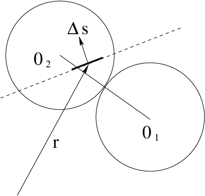
Let us first analyze the pressure tensor case. Let us consider a surface element, Δ​𝐬\Delta\mathbf{s}, centered at 𝐫\mathbf{r} and two particles at contact in such a way that the line joining the two centers cross the surface (see Fig. 2). When the collision takes place, the variation of the momentum of particle 22 is

Δ​p2,i=m⁡(𝝈^⋅𝐯12)​σ^i.\Delta p_{2,i}=m(\boldsymbol{\hat{\sigma}}\cdot\mathbf{v}_{12})\hat{\sigma}_{i}. (65)
Refer to caption
Figure 2: Sketch of a typical collision that contributes to the flux through Δ​𝐬\Delta\mathbf{s}. It is assumed that particles 11 and 22 have the centers at 010_{1} and 020_{2} respectively.

It is assumed that, in order to evaluate the flux, Δ​p2,i\Delta p_{2,i} cross the surface through the intersection of the surface with the line joining the two particles. To calculate the collisional contribution to the flux, we have to consider all the possible collisions of this kind with its corresponding Δ​p2,i\Delta p_{2,i}. The surface divides the space in two regions; of course, the centers of the particles must be in different regions. We will consider that particle 22 is in the region pointed by Δ​𝐬\Delta\mathbf{s}, as in the Figure. The center of particle 11 can be parameterized by

𝐫1​(λ,𝝈^)=𝐫+λ​σ​𝝈^,\mathbf{r}_{1}(\lambda,\boldsymbol{\hat{\sigma}})=\mathbf{r}+\lambda\sigma\boldsymbol{\hat{\sigma}}, (66)

with λ∈(0,1)\lambda\in(0,1) and 𝝈^\boldsymbol{\hat{\sigma}} a unitary vector of arbitrary orientation, but compatible with Δ​𝐬\Delta\mathbf{s}, i.e. 𝝈^⋅Δ​𝐬<0\boldsymbol{\hat{\sigma}}\cdot\Delta\mathbf{s}<0. In these conditions, particle 22 must be in a solid angle

Δ​σ^2=|𝝈^⋅Δ​𝐬|(λ​σ)d−1,\Delta\hat{\sigma}_{2}=\frac{\lvert\boldsymbol{\hat{\sigma}}\cdot\Delta\mathbf{s}\rvert}{(\lambda\sigma)^{d-1}}, (67)

around

𝐫2​(λ,𝝈^)=𝐫−(1−λ)​σ​𝝈^.\mathbf{r}_{2}(\lambda,\boldsymbol{\hat{\sigma}})=\mathbf{r}-(1-\lambda)\sigma\boldsymbol{\hat{\sigma}}. (68)

Note that we have used the same notation for the 𝝈^\boldsymbol{\hat{\sigma}} of the collision in Eq. (65), and for the parameter to specify the position of particle 11 in Eq. (66). This can be done because its difference is of order Δ​σ^2\Delta\hat{\sigma}_{2}.

Let us consider that particle 11 is in the volume element Δ​𝐫1=(λ​σ)d−1​Δ​(λ​σ)​Δ​𝝈^\Delta\mathbf{r}_{1}=(\lambda\sigma)^{d-1}\Delta(\lambda\sigma)\Delta\boldsymbol{\hat{\sigma}} parameterized by (λ,𝝈^)(\lambda,\boldsymbol{\hat{\sigma}}). Hence, if particle 22 collides with particle 11 in the time interval Δ​t\Delta t with 𝝈^\boldsymbol{\hat{\sigma}}, it is in the volume element Δ​𝐫2=σd−1​Δ​σ^2​|𝐯12⋅𝝈^|​Δ​t\Delta\mathbf{r}_{2}=\sigma^{d-1}\Delta\hat{\sigma}_{2}\lvert\mathbf{v}_{12}\cdot\boldsymbol{\hat{\sigma}}\rvert\Delta t. Then, the total number of collisions that contribute to the flux for given 𝐯1\mathbf{v}_{1} and 𝐯2\mathbf{v}_{2} is

θ(−𝐯12⋅𝝈^)f2[𝐫1(λ,𝝈^),𝐯1,𝐫2(λ,𝝈^),𝐯2]Δ𝐫1Δ𝐯1Δ𝐫2Δ𝐯2\displaystyle\theta(-\mathbf{v}_{12}\cdot\boldsymbol{\hat{\sigma}})f_{2}[\mathbf{r}_{1}(\lambda,\boldsymbol{\hat{\sigma}}),\mathbf{v}_{1},\mathbf{r}_{2}(\lambda,\boldsymbol{\hat{\sigma}}),\mathbf{v}_{2}]\Delta\mathbf{r}_{1}\Delta\mathbf{v}_{1}\Delta\mathbf{r}_{2}\Delta\mathbf{v}_{2}
=σdθ(−𝐯12⋅𝝈^)f2[𝐫1(λ,𝝈^),𝐯1,𝐫2(λ,𝝈^),𝐯2]|𝝈^⋅Δ𝐬||𝐯12⋅𝝈^|Δ𝐯1Δ𝐯2Δ𝝈^ΔλΔt.\displaystyle=\sigma^{d}\theta(-\mathbf{v}_{12}\cdot\boldsymbol{\hat{\sigma}})f_{2}[\mathbf{r}_{1}(\lambda,\boldsymbol{\hat{\sigma}}),\mathbf{v}_{1},\mathbf{r}_{2}(\lambda,\boldsymbol{\hat{\sigma}}),\mathbf{v}_{2}]\lvert\boldsymbol{\hat{\sigma}}\cdot\Delta\mathbf{s}\rvert\lvert\mathbf{v}_{12}\cdot\boldsymbol{\hat{\sigma}}\rvert\Delta\mathbf{v}_{1}\Delta\mathbf{v}_{2}\Delta\boldsymbol{\hat{\sigma}}\Delta\lambda\Delta t. (69)

Let us take Δ​𝐬=Δ​s​𝐞j\Delta\mathbf{s}=\Delta s\mathbf{e}_{j} where 𝐞j\mathbf{e}_{j} is a unit vector in the direction of one of our coordinate axes. The amount of momentum that travels through the surface in the direction of Δ​𝐬\Delta\mathbf{s} per unit time and area due to collisions of particles with velocities 𝐯1\mathbf{v}_{1} and 𝐯2\mathbf{v}_{2} is then

ΔPi​j(c)=mσdθ(−𝐯12⋅𝝈^)f2[𝐫1(λ,𝝈^),𝐯1,𝐫2(λ,𝝈^),𝐯2]σ^iσ^j(𝐯12⋅𝝈^)2Δ𝐯1Δ𝐯2Δ𝝈^Δλ,\Delta P_{ij}^{(c)}=m\sigma^{d}\theta(-\mathbf{v}_{12}\cdot\boldsymbol{\hat{\sigma}})f_{2}[\mathbf{r}_{1}(\lambda,\boldsymbol{\hat{\sigma}}),\mathbf{v}_{1},\mathbf{r}_{2}(\lambda,\boldsymbol{\hat{\sigma}}),\mathbf{v}_{2}]\hat{\sigma}_{i}\hat{\sigma}_{j}(\mathbf{v}_{12}\cdot\boldsymbol{\hat{\sigma}})^{2}\Delta\mathbf{v}_{1}\Delta\mathbf{v}_{2}\Delta\boldsymbol{\hat{\sigma}}\Delta\lambda, (70)

where we have taken into account that |𝐯12⋅𝝈^|=−𝐯12⋅𝝈^\lvert\mathbf{v}_{12}\cdot\boldsymbol{\hat{\sigma}}\rvert=-\mathbf{v}_{12}\cdot\boldsymbol{\hat{\sigma}} and |σ^j|=−σ^j\lvert\hat{\sigma}_{j}\rvert=-\hat{\sigma}_{j}. The net collisional pressure tensor is obtained integrating in Eq. (70) for all the allowed collisions.

Far from the boundary, when there are not geometrical constraints, the result is

Pi​j(c)=mσd∫d𝐯1∫d𝐯2∫01dλ∫σ^j<0d𝝈^θ(−𝐯12⋅𝝈^)f2[𝐫1(λ,𝝈^),𝐯1,𝐫2(λ,𝝈^),𝐯2]σ^iσ^j(𝐯12⋅𝝈^)2.P_{ij}^{(c)}=m\sigma^{d}\int d\mathbf{v}_{1}\int d\mathbf{v}_{2}\int_{0}^{1}d\lambda\int_{\hat{\sigma}_{j}<0}d\boldsymbol{\hat{\sigma}}\theta(-\mathbf{v}_{12}\cdot\boldsymbol{\hat{\sigma}})f_{2}[\mathbf{r}_{1}(\lambda,\boldsymbol{\hat{\sigma}}),\mathbf{v}_{1},\mathbf{r}_{2}(\lambda,\boldsymbol{\hat{\sigma}}),\mathbf{v}_{2}]\hat{\sigma}_{i}\hat{\sigma}_{j}(\mathbf{v}_{12}\cdot\boldsymbol{\hat{\sigma}})^{2}. (71)

The integration can also be done summing for σ^j>0\hat{\sigma}_{j}>0 but, then, the amount of momentum that crosses the surface is Δ​p1,i=−Δ​p2,i\Delta p_{1,i}=-\Delta p_{2,i}, so that

Pi​j(c)=mσd∫d𝐯1∫d𝐯2∫01dλ∫σ^j>0d𝝈^θ(−𝐯12⋅𝝈^)f2[𝐫1(λ,𝝈^),𝐯1,𝐫2(λ,𝝈^),𝐯2]σ^iσ^j(𝐯12⋅𝝈^)2,P_{ij}^{(c)}=m\sigma^{d}\int d\mathbf{v}_{1}\int d\mathbf{v}_{2}\int_{0}^{1}d\lambda\int_{\hat{\sigma}_{j}>0}d\boldsymbol{\hat{\sigma}}\theta(-\mathbf{v}_{12}\cdot\boldsymbol{\hat{\sigma}})f_{2}[\mathbf{r}_{1}(\lambda,\boldsymbol{\hat{\sigma}}),\mathbf{v}_{1},\mathbf{r}_{2}(\lambda,\boldsymbol{\hat{\sigma}}),\mathbf{v}_{2}]\hat{\sigma}_{i}\hat{\sigma}_{j}(\mathbf{v}_{12}\cdot\boldsymbol{\hat{\sigma}})^{2}, (72)

because, in this case, |σ^j|=σ^j\lvert\hat{\sigma}_{j}\rvert=\hat{\sigma}_{j}. Hence, we can re-write Eq. (71) as

Pi​j(c)=m2σd∫d𝐯1∫d𝐯2∫01dλ∫d𝝈^θ(−𝐯12⋅𝝈^)f2[𝐫1(λ,𝝈^),𝐯1,𝐫2(λ,𝝈^),𝐯2]σ^iσ^j(𝐯12⋅𝝈^)2,P_{ij}^{(c)}=\frac{m}{2}\sigma^{d}\int d\mathbf{v}_{1}\int d\mathbf{v}_{2}\int_{0}^{1}d\lambda\int d\boldsymbol{\hat{\sigma}}\theta(-\mathbf{v}_{12}\cdot\boldsymbol{\hat{\sigma}})f_{2}[\mathbf{r}_{1}(\lambda,\boldsymbol{\hat{\sigma}}),\mathbf{v}_{1},\mathbf{r}_{2}(\lambda,\boldsymbol{\hat{\sigma}}),\mathbf{v}_{2}]\hat{\sigma}_{i}\hat{\sigma}_{j}(\mathbf{v}_{12}\cdot\boldsymbol{\hat{\sigma}})^{2}, (73)

that coincides with the expression derived in [24] for d=3d=3 when the factorization for f2f_{2} given by Eq. (16) is used.

If there are geometrical constraints, we proceed similarly. Integrating in Eq. (70) for the allowed collisions, it is obtained

Pi​j(c)=mσd∫d𝐯1∫d𝐯2∫∫Σ−dλd𝝈^θ(−𝐯12⋅𝝈^)f2[𝐫1(λ,𝝈^),𝐯1,𝐫2(λ,𝝈^),𝐯2]σ^iσ^j(𝐯12⋅𝝈^)2,P_{ij}^{(c)}=m\sigma^{d}\int d\mathbf{v}_{1}\int d\mathbf{v}_{2}\int\int_{\Sigma^{-}}d\lambda d\boldsymbol{\hat{\sigma}}\theta(-\mathbf{v}_{12}\cdot\boldsymbol{\hat{\sigma}})f_{2}[\mathbf{r}_{1}(\lambda,\boldsymbol{\hat{\sigma}}),\mathbf{v}_{1},\mathbf{r}_{2}(\lambda,\boldsymbol{\hat{\sigma}}),\mathbf{v}_{2}]\hat{\sigma}_{i}\hat{\sigma}_{j}(\mathbf{v}_{12}\cdot\boldsymbol{\hat{\sigma}})^{2}, (74)

where the region of integration in (λ,𝝈^)(\lambda,\boldsymbol{\hat{\sigma}}) is

Σ−={(λ,𝝈^)|𝝈^∈Ωdwithσ^j<0&0≤λ≤1&𝐫1(λ,𝝈^)∈V&𝐫2(λ,𝝈^)∈V}.\Sigma^{-}=\{(\lambda,\boldsymbol{\hat{\sigma}})\lvert\boldsymbol{\hat{\sigma}}\in\Omega_{d}\quad\textrm{with}\quad\hat{\sigma}_{j}<0\quad\&\quad 0\leq\lambda\leq 1\quad\&\quad\mathbf{r}_{1}(\lambda,\boldsymbol{\hat{\sigma}})\in V\quad\&\quad\mathbf{r}_{2}(\lambda,\boldsymbol{\hat{\sigma}})\in V\}. (75)

Pi​j(c)P_{ij}^{(c)} can also be calculated summing for σ^j>0\hat{\sigma}_{j}>0 but, then, the amount of momentum that crosses the surface is Δ​p1,i=−Δ​p2,i\Delta p_{1,i}=-\Delta p_{2,i}, so that

Pi​j(c)=mσd∫d𝐯1∫d𝐯2∫∫Σ+dλd𝝈^θ(−𝐯12⋅𝝈^)f2[𝐫1(λ,𝝈^),𝐯1,𝐫2(λ,𝝈^),𝐯2]σ^iσ^j(𝐯12⋅𝝈^)2,P_{ij}^{(c)}=m\sigma^{d}\int d\mathbf{v}_{1}\int d\mathbf{v}_{2}\int\int_{\Sigma^{+}}d\lambda d\boldsymbol{\hat{\sigma}}\theta(-\mathbf{v}_{12}\cdot\boldsymbol{\hat{\sigma}})f_{2}[\mathbf{r}_{1}(\lambda,\boldsymbol{\hat{\sigma}}),\mathbf{v}_{1},\mathbf{r}_{2}(\lambda,\boldsymbol{\hat{\sigma}}),\mathbf{v}_{2}]\hat{\sigma}_{i}\hat{\sigma}_{j}(\mathbf{v}_{12}\cdot\boldsymbol{\hat{\sigma}})^{2}, (76)

where the region of integration in (λ,𝝈^)(\lambda,\boldsymbol{\hat{\sigma}}) is

Σ+={(λ,𝝈^)|𝝈^∈Ωdwithσ^j>0&0≤λ≤1&𝐫1(λ,𝝈^)∈V&𝐫2(λ,𝝈^)∈V}.\Sigma^{+}=\{(\lambda,\boldsymbol{\hat{\sigma}})\lvert\boldsymbol{\hat{\sigma}}\in\Omega_{d}\quad\textrm{with}\quad\hat{\sigma}_{j}>0\quad\&\quad 0\leq\lambda\leq 1\quad\&\quad\mathbf{r}_{1}(\lambda,\boldsymbol{\hat{\sigma}})\in V\quad\&\quad\mathbf{r}_{2}(\lambda,\boldsymbol{\hat{\sigma}})\in V\}. (77)

Hence, we can re-write Eq. (74) as

Pi​j(c)=m2σd∫d𝐯1∫d𝐯2∫∫Σdλd𝝈^θ(−𝐯12⋅𝝈^)f2[𝐫1(λ,𝝈^),𝐯1,𝐫2(λ,𝝈^),𝐯2]σ^iσ^j(𝐯12⋅𝝈^)2,P_{ij}^{(c)}=\frac{m}{2}\sigma^{d}\int d\mathbf{v}_{1}\int d\mathbf{v}_{2}\int\int_{\Sigma}d\lambda d\boldsymbol{\hat{\sigma}}\theta(-\mathbf{v}_{12}\cdot\boldsymbol{\hat{\sigma}})f_{2}[\mathbf{r}_{1}(\lambda,\boldsymbol{\hat{\sigma}}),\mathbf{v}_{1},\mathbf{r}_{2}(\lambda,\boldsymbol{\hat{\sigma}}),\mathbf{v}_{2}]\hat{\sigma}_{i}\hat{\sigma}_{j}(\mathbf{v}_{12}\cdot\boldsymbol{\hat{\sigma}})^{2}, (78)

where the region of integration in (λ,𝝈^)(\lambda,\boldsymbol{\hat{\sigma}}) is

Σ={(λ,𝝈^)|𝝈^∈Ωd&0≤λ≤1&𝐫1(λ,𝝈^)∈V&𝐫2(λ,𝝈^)∈V}.\Sigma=\{(\lambda,\boldsymbol{\hat{\sigma}})\lvert\boldsymbol{\hat{\sigma}}\in\Omega_{d}\quad\&\quad 0\leq\lambda\leq 1\quad\&\quad\mathbf{r}_{1}(\lambda,\boldsymbol{\hat{\sigma}})\in V\quad\&\quad\mathbf{r}_{2}(\lambda,\boldsymbol{\hat{\sigma}})\in V\}. (79)

To calculate the collisional contribution to the energy flux, JE,j(c)J_{E,j}^{(c)}, the analysis is similar, but taking into account that, when the collision takes place, the variation of the energy of particle 22 is

Δ​e2,i=m2​(𝝈^⋅𝐯12)2+m⁡(𝝈^⋅𝐯12)​(𝝈^⋅𝐯2).\Delta e_{2,i}=\frac{m}{2}(\boldsymbol{\hat{\sigma}}\cdot\mathbf{v}_{12})^{2}+m(\boldsymbol{\hat{\sigma}}\cdot\mathbf{v}_{12})(\boldsymbol{\hat{\sigma}}\cdot\mathbf{v}_{2}). (80)

Once JE,j(c)J_{E,j}^{(c)} is calculated, the heat flux is expressed as qj(c)=JE,j(c)−∑iui​Pi​j(c)q_{j}^{(c)}=J_{E,j}^{(c)}-\sum_{i}u_{i}P_{ij}^{(c)}.

Appendix B Evaluation of the divergence of the collisional fluxes

As in the previous Appendix, we focus on the pressure tensor because the heat flux case is similar. Let us first re-write the collisional pressure tensor given by Eq. (36) in the form

Pi​j(c)(𝐫,t)=m2σd∫d𝐯1∫d𝐯2∫d𝝈^∫λ1​(𝐫,𝝈^)λ2​(𝐫,𝝈^)dλθ(−𝐯12⋅𝝈^)f2[𝐫1(λ,𝝈^),𝐯1,𝐫2(λ,𝝈^),𝐯2,t](𝐯12⋅𝝈^)2σi^σj^,P_{ij}^{(c)}(\mathbf{r},t)=\frac{m}{2}\sigma^{d}\int d\mathbf{v}_{1}\int d\mathbf{v}_{2}\int d\boldsymbol{\hat{\sigma}}\int_{\lambda_{1}(\mathbf{r},\boldsymbol{\hat{\sigma}})}^{\lambda_{2}(\mathbf{r},\boldsymbol{\hat{\sigma}})}d\lambda\theta(-\mathbf{v}_{12}\cdot\boldsymbol{\hat{\sigma}})f_{2}[\mathbf{r}_{1}(\lambda,\boldsymbol{\hat{\sigma}}),\mathbf{v}_{1},\mathbf{r}_{2}(\lambda,\boldsymbol{\hat{\sigma}}),\mathbf{v}_{2},t](\mathbf{v}_{12}\cdot\boldsymbol{\hat{\sigma}})^{2}\hat{\sigma_{i}}\hat{\sigma_{j}}, (81)

where λ1​(𝐫,𝝈^)\lambda_{1}(\mathbf{r},\boldsymbol{\hat{\sigma}}) and λ2​(𝐫,𝝈^)\lambda_{2}(\mathbf{r},\boldsymbol{\hat{\sigma}}) are such that σ​λ1​(𝐫,𝝈^)\sigma\lambda_{1}(\mathbf{r},\boldsymbol{\hat{\sigma}}) and σ​λ2​(𝐫,𝝈^)\sigma\lambda_{2}(\mathbf{r},\boldsymbol{\hat{\sigma}}) are the minimum and maximum distance from 𝐫\mathbf{r} to 𝐫1​(λ,𝝈^)\mathbf{r}_{1}(\lambda,\boldsymbol{\hat{\sigma}}) respectively, for a given orientation, 𝝈^\boldsymbol{\hat{\sigma}}. In the bulk of the system, we trivially have λ1​(𝐫,𝝈^)=0\lambda_{1}(\mathbf{r},\boldsymbol{\hat{\sigma}})=0 and λ2​(𝐫,𝝈^)=1\lambda_{2}(\mathbf{r},\boldsymbol{\hat{\sigma}})=1, for all 𝝈^\boldsymbol{\hat{\sigma}}, but closed to the boundary these functions depend on the geometry of it.

Taking into account Eq. (81), the divergence of Pi​j(c)P_{ij}^{(c)} can be expressed as

∂∂𝐫⋅Pi​j(c)​(𝐫)\displaystyle\frac{\partial}{\partial\mathbf{r}}\cdot P_{ij}^{(c)}(\mathbf{r})
=m2σd∫d𝐯1∫d𝐯2∫d𝝈^θ(−𝐯12⋅𝝈^)(𝐯12⋅𝝈^)2𝝈^𝝈^⋅∂∂𝐫λ2f2[𝐫1(λ2,𝝈^),𝐯1,𝐫2(λ2,𝝈^),𝐯2]\displaystyle=\frac{m}{2}\sigma^{d}\int d\mathbf{v}_{1}\int d\mathbf{v}_{2}\int d\boldsymbol{\hat{\sigma}}\theta(-\mathbf{v}_{12}\cdot\boldsymbol{\hat{\sigma}})(\mathbf{v}_{12}\cdot\boldsymbol{\hat{\sigma}})^{2}\boldsymbol{\hat{\sigma}}\boldsymbol{\hat{\sigma}}\cdot\frac{\partial}{\partial\mathbf{r}}\lambda_{2}f_{2}[\mathbf{r}_{1}(\lambda_{2},\boldsymbol{\hat{\sigma}}),\mathbf{v}_{1},\mathbf{r}_{2}(\lambda_{2},\boldsymbol{\hat{\sigma}}),\mathbf{v}_{2}]
−m2σd∫d𝐯1∫d𝐯2∫d𝝈^θ(−𝐯12⋅𝝈^)(𝐯12⋅𝝈^)2𝝈^𝝈^⋅∂∂𝐫λ1f2[𝐫1(λ1,𝝈^),𝐯1,𝐫2(λ1,𝝈^),𝐯2]\displaystyle-\frac{m}{2}\sigma^{d}\int d\mathbf{v}_{1}\int d\mathbf{v}_{2}\int d\boldsymbol{\hat{\sigma}}\theta(-\mathbf{v}_{12}\cdot\boldsymbol{\hat{\sigma}})(\mathbf{v}_{12}\cdot\boldsymbol{\hat{\sigma}})^{2}\boldsymbol{\hat{\sigma}}\boldsymbol{\hat{\sigma}}\cdot\frac{\partial}{\partial\mathbf{r}}\lambda_{1}f_{2}[\mathbf{r}_{1}(\lambda_{1},\boldsymbol{\hat{\sigma}}),\mathbf{v}_{1},\mathbf{r}_{2}(\lambda_{1},\boldsymbol{\hat{\sigma}}),\mathbf{v}_{2}]
+m2σd∫d𝐯1∫d𝐯2∫d𝝈^θ(−𝐯12⋅𝝈^)(𝐯12⋅𝝈^)2𝝈^∫λ1​(𝐫,𝝈^)λ2​(𝐫,𝝈^)dλ𝝈^⋅∂∂𝐫f2[𝐫1(λ,𝝈^),𝐯1,𝐫2(λ,𝝈^),𝐯2].\displaystyle+\frac{m}{2}\sigma^{d}\int d\mathbf{v}_{1}\int d\mathbf{v}_{2}\int d\boldsymbol{\hat{\sigma}}\theta(-\mathbf{v}_{12}\cdot\boldsymbol{\hat{\sigma}})(\mathbf{v}_{12}\cdot\boldsymbol{\hat{\sigma}})^{2}\boldsymbol{\hat{\sigma}}\int_{\lambda_{1}(\mathbf{r},\boldsymbol{\hat{\sigma}})}^{\lambda_{2}(\mathbf{r},\boldsymbol{\hat{\sigma}})}d\lambda\boldsymbol{\hat{\sigma}}\cdot\frac{\partial}{\partial\mathbf{r}}f_{2}[\mathbf{r}_{1}(\lambda,\boldsymbol{\hat{\sigma}}),\mathbf{v}_{1},\mathbf{r}_{2}(\lambda,\boldsymbol{\hat{\sigma}}),\mathbf{v}_{2}].

Taking into account that

∂∂λ​f2​[𝐫1​(λ,𝝈^),𝐯1,𝐫2​(λ,𝝈^),𝐯2]=𝝈⋅∂∂𝐫​f2​[𝐫1​(λ,𝝈^),𝐯1,𝐫2​(λ,𝝈^),𝐯2],\frac{\partial}{\partial\lambda}f_{2}[\mathbf{r}_{1}(\lambda,\boldsymbol{\hat{\sigma}}),\mathbf{v}_{1},\mathbf{r}_{2}(\lambda,\boldsymbol{\hat{\sigma}}),\mathbf{v}_{2}]=\boldsymbol{\sigma}\cdot\frac{\partial}{\partial\mathbf{r}}f_{2}[\mathbf{r}_{1}(\lambda,\boldsymbol{\hat{\sigma}}),\mathbf{v}_{1},\mathbf{r}_{2}(\lambda,\boldsymbol{\hat{\sigma}}),\mathbf{v}_{2}], (83)

the last term of the r.h.s. of Eq. (B) can be written as

m2σd∫d𝐯1∫d𝐯2∫d𝝈^θ(−𝐯12⋅𝝈^)(𝐯12⋅𝝈^)2𝝈^∫λ1​(𝐫,𝝈^)λ2​(𝐫,𝝈^)dλ𝝈^⋅∂∂𝐫f2[𝐫1(λ,𝝈^),𝐯1,𝐫2(λ,𝝈^),𝐯2]\displaystyle\frac{m}{2}\sigma^{d}\int d\mathbf{v}_{1}\int d\mathbf{v}_{2}\int d\boldsymbol{\hat{\sigma}}\theta(-\mathbf{v}_{12}\cdot\boldsymbol{\hat{\sigma}})(\mathbf{v}_{12}\cdot\boldsymbol{\hat{\sigma}})^{2}\boldsymbol{\hat{\sigma}}\int_{\lambda_{1}(\mathbf{r},\boldsymbol{\hat{\sigma}})}^{\lambda_{2}(\mathbf{r},\boldsymbol{\hat{\sigma}})}d\lambda\boldsymbol{\hat{\sigma}}\cdot\frac{\partial}{\partial\mathbf{r}}f_{2}[\mathbf{r}_{1}(\lambda,\boldsymbol{\hat{\sigma}}),\mathbf{v}_{1},\mathbf{r}_{2}(\lambda,\boldsymbol{\hat{\sigma}}),\mathbf{v}_{2}]
=m2σd−1∫d𝐯1∫d𝐯2∫d𝝈^θ(−𝐯12⋅𝝈^)(𝐯12⋅𝝈^)2𝝈^f2[𝐫1(λ2,𝝈^),𝐯1,𝐫2(λ2,𝝈^),𝐯2]\displaystyle=\frac{m}{2}\sigma^{d-1}\int d\mathbf{v}_{1}\int d\mathbf{v}_{2}\int d\boldsymbol{\hat{\sigma}}\theta(-\mathbf{v}_{12}\cdot\boldsymbol{\hat{\sigma}})(\mathbf{v}_{12}\cdot\boldsymbol{\hat{\sigma}})^{2}\boldsymbol{\hat{\sigma}}f_{2}[\mathbf{r}_{1}(\lambda_{2},\boldsymbol{\hat{\sigma}}),\mathbf{v}_{1},\mathbf{r}_{2}(\lambda_{2},\boldsymbol{\hat{\sigma}}),\mathbf{v}_{2}]
−m2σd−1∫d𝐯1∫d𝐯2∫d𝝈^θ(−𝐯12⋅𝝈^)(𝐯12⋅𝝈^)2𝝈^f2[𝐫1(λ1,𝝈^),𝐯1,𝐫2(λ1,𝝈^),𝐯2].\displaystyle-\frac{m}{2}\sigma^{d-1}\int d\mathbf{v}_{1}\int d\mathbf{v}_{2}\int d\boldsymbol{\hat{\sigma}}\theta(-\mathbf{v}_{12}\cdot\boldsymbol{\hat{\sigma}})(\mathbf{v}_{12}\cdot\boldsymbol{\hat{\sigma}})^{2}\boldsymbol{\hat{\sigma}}f_{2}[\mathbf{r}_{1}(\lambda_{1},\boldsymbol{\hat{\sigma}}),\mathbf{v}_{1},\mathbf{r}_{2}(\lambda_{1},\boldsymbol{\hat{\sigma}}),\mathbf{v}_{2}].

Changing variables,

𝐯1\displaystyle\mathbf{v}_{1} ↔\displaystyle\leftrightarrow 𝐯2,\displaystyle\mathbf{v}_{2}, (85)
𝝈^\displaystyle\boldsymbol{\hat{\sigma}} →\displaystyle\to −𝝈^,\displaystyle-\boldsymbol{\hat{\sigma}}, (86)

in the second term of the r.h.s., it is obtained

m2σd−1∫d𝐯1∫d𝐯2∫d𝝈^θ(−𝐯12⋅𝝈^)(𝐯12⋅𝝈^)2𝝈^f2[𝐫1(λ1,𝝈^),𝐯1,𝐫2(λ1,𝝈^),𝐯2].\displaystyle\frac{m}{2}\sigma^{d-1}\int d\mathbf{v}_{1}\int d\mathbf{v}_{2}\int d\boldsymbol{\hat{\sigma}}\theta(-\mathbf{v}_{12}\cdot\boldsymbol{\hat{\sigma}})(\mathbf{v}_{12}\cdot\boldsymbol{\hat{\sigma}})^{2}\boldsymbol{\hat{\sigma}}f_{2}[\mathbf{r}_{1}(\lambda_{1},\boldsymbol{\hat{\sigma}}),\mathbf{v}_{1},\mathbf{r}_{2}(\lambda_{1},\boldsymbol{\hat{\sigma}}),\mathbf{v}_{2}].
=−m2σd−1∫d𝐯1∫d𝐯2∫d𝝈^θ(−𝐯12⋅𝝈^)(𝐯12⋅𝝈^)2𝝈^f2[𝐫1(λ2,𝝈^),𝐯1,𝐫2(λ2,𝝈^),𝐯2],\displaystyle=-\frac{m}{2}\sigma^{d-1}\int d\mathbf{v}_{1}\int d\mathbf{v}_{2}\int d\boldsymbol{\hat{\sigma}}\theta(-\mathbf{v}_{12}\cdot\boldsymbol{\hat{\sigma}})(\mathbf{v}_{12}\cdot\boldsymbol{\hat{\sigma}})^{2}\boldsymbol{\hat{\sigma}}f_{2}[\mathbf{r}_{1}(\lambda_{2},\boldsymbol{\hat{\sigma}}),\mathbf{v}_{1},\mathbf{r}_{2}(\lambda_{2},\boldsymbol{\hat{\sigma}}),\mathbf{v}_{2}],

where it has taken into account that

𝐫1​[λ1​(𝐫,−𝝈^),−𝝈^]\displaystyle\mathbf{r}_{1}[\lambda_{1}(\mathbf{r},-\boldsymbol{\hat{\sigma}}),-\boldsymbol{\hat{\sigma}}] =\displaystyle= 𝐫2​[λ2​(𝐫,𝝈^),𝝈^],\displaystyle\mathbf{r}_{2}[\lambda_{2}(\mathbf{r},\boldsymbol{\hat{\sigma}}),\boldsymbol{\hat{\sigma}}], (88)
𝐫2​[λ1​(𝐫,−𝝈^),−𝝈^]\displaystyle\mathbf{r}_{2}[\lambda_{1}(\mathbf{r},-\boldsymbol{\hat{\sigma}}),-\boldsymbol{\hat{\sigma}}] =\displaystyle= 𝐫1​[λ2​(𝐫,𝝈^),𝝈^].\displaystyle\mathbf{r}_{1}[\lambda_{2}(\mathbf{r},\boldsymbol{\hat{\sigma}}),\boldsymbol{\hat{\sigma}}]. (89)

So, we have

m2σd∫d𝐯1∫d𝐯2∫d𝝈^θ(−𝐯12⋅𝝈^)(𝐯12⋅𝝈^)2𝝈^∫λ1​(𝐫,𝝈^)λ2​(𝐫,𝝈^)dλ𝝈^⋅∂∂𝐫f2[𝐫1(λ,𝝈^),𝐯1,𝐫2(λ,𝝈^),𝐯2]\displaystyle\frac{m}{2}\sigma^{d}\int d\mathbf{v}_{1}\int d\mathbf{v}_{2}\int d\boldsymbol{\hat{\sigma}}\theta(-\mathbf{v}_{12}\cdot\boldsymbol{\hat{\sigma}})(\mathbf{v}_{12}\cdot\boldsymbol{\hat{\sigma}})^{2}\boldsymbol{\hat{\sigma}}\int_{\lambda_{1}(\mathbf{r},\boldsymbol{\hat{\sigma}})}^{\lambda_{2}(\mathbf{r},\boldsymbol{\hat{\sigma}})}d\lambda\boldsymbol{\hat{\sigma}}\cdot\frac{\partial}{\partial\mathbf{r}}f_{2}[\mathbf{r}_{1}(\lambda,\boldsymbol{\hat{\sigma}}),\mathbf{v}_{1},\mathbf{r}_{2}(\lambda,\boldsymbol{\hat{\sigma}}),\mathbf{v}_{2}]
=mσd−1∫d𝐯1∫d𝐯2∫d𝝈^θ(−𝐯12⋅𝝈^)(𝐯12⋅𝝈^)2𝝈^f2[𝐫1(λ2,𝝈^),𝐯1,𝐫2(λ2,𝝈^),𝐯2].\displaystyle=m\sigma^{d-1}\int d\mathbf{v}_{1}\int d\mathbf{v}_{2}\int d\boldsymbol{\hat{\sigma}}\theta(-\mathbf{v}_{12}\cdot\boldsymbol{\hat{\sigma}})(\mathbf{v}_{12}\cdot\boldsymbol{\hat{\sigma}})^{2}\boldsymbol{\hat{\sigma}}f_{2}[\mathbf{r}_{1}(\lambda_{2},\boldsymbol{\hat{\sigma}}),\mathbf{v}_{1},\mathbf{r}_{2}(\lambda_{2},\boldsymbol{\hat{\sigma}}),\mathbf{v}_{2}].

Performing the same change of variables in the second term of the r.h.s. of Eq. (B), it is obtained

m2σd∫d𝐯1∫d𝐯2∫d𝝈^θ(−𝐯12⋅𝝈^)(𝐯12⋅𝝈^)2𝝈^𝝈^⋅∂∂𝐫λ1f2[𝐫1(λ1,𝝈^),𝐯1,𝐫2(λ1,𝝈^),𝐯2]\displaystyle\frac{m}{2}\sigma^{d}\int d\mathbf{v}_{1}\int d\mathbf{v}_{2}\int d\boldsymbol{\hat{\sigma}}\theta(-\mathbf{v}_{12}\cdot\boldsymbol{\hat{\sigma}})(\mathbf{v}_{12}\cdot\boldsymbol{\hat{\sigma}})^{2}\boldsymbol{\hat{\sigma}}\boldsymbol{\hat{\sigma}}\cdot\frac{\partial}{\partial\mathbf{r}}\lambda_{1}f_{2}[\mathbf{r}_{1}(\lambda_{1},\boldsymbol{\hat{\sigma}}),\mathbf{v}_{1},\mathbf{r}_{2}(\lambda_{1},\boldsymbol{\hat{\sigma}}),\mathbf{v}_{2}]
=−m2σd∫d𝐯1∫d𝐯2∫d𝝈^θ(−𝐯12⋅𝝈^)(𝐯12⋅𝝈^)2𝝈^𝝈^⋅∂∂𝐫λ2f2[𝐫1(λ2,𝝈^),𝐯1,𝐫2(λ2,𝝈^),𝐯2].\displaystyle=-\frac{m}{2}\sigma^{d}\int d\mathbf{v}_{1}\int d\mathbf{v}_{2}\int d\boldsymbol{\hat{\sigma}}\theta(-\mathbf{v}_{12}\cdot\boldsymbol{\hat{\sigma}})(\mathbf{v}_{12}\cdot\boldsymbol{\hat{\sigma}})^{2}\boldsymbol{\hat{\sigma}}\boldsymbol{\hat{\sigma}}\cdot\frac{\partial}{\partial\mathbf{r}}\lambda_{2}f_{2}[\mathbf{r}_{1}(\lambda_{2},\boldsymbol{\hat{\sigma}}),\mathbf{v}_{1},\mathbf{r}_{2}(\lambda_{2},\boldsymbol{\hat{\sigma}}),\mathbf{v}_{2}].

By substituting Eqs. (B) and (B) into Eq. (B), it is obtained

∂∂𝐫⋅Pi​j(c)​(𝐫)\displaystyle\frac{\partial}{\partial\mathbf{r}}\cdot P_{ij}^{(c)}(\mathbf{r})
=mσd−1∫d𝐯1∫d𝐯2∫d𝝈^θ(−𝐯12⋅𝝈^)(𝐯12⋅𝝈^)2𝝈^[1+𝝈⋅∂∂𝐫λ2]f2[𝐫1(λ2,𝝈^),𝐯1,𝐫2(λ2,𝝈^),𝐯2].\displaystyle=m\sigma^{d-1}\int d\mathbf{v}_{1}\int d\mathbf{v}_{2}\int d\boldsymbol{\hat{\sigma}}\theta(-\mathbf{v}_{12}\cdot\boldsymbol{\hat{\sigma}})(\mathbf{v}_{12}\cdot\boldsymbol{\hat{\sigma}})^{2}\boldsymbol{\hat{\sigma}}\left[1+\boldsymbol{\sigma}\cdot\frac{\partial}{\partial\mathbf{r}}\lambda_{2}\right]f_{2}[\mathbf{r}_{1}(\lambda_{2},\boldsymbol{\hat{\sigma}}),\mathbf{v}_{1},\mathbf{r}_{2}(\lambda_{2},\boldsymbol{\hat{\sigma}}),\mathbf{v}_{2}].

Now, let us analyze the function 1+𝝈⋅∂∂𝐫​λ21+\boldsymbol{\sigma}\cdot\frac{\partial}{\partial\mathbf{r}}\lambda_{2}. Let us first consider the simplest case of a plane located at z=−σ/2z=-\sigma/2. If 𝝈^∈Ω⁡(𝐫)\boldsymbol{\hat{\sigma}}\in\Omega(\mathbf{r}), then λ2​(𝐫,𝝈^)=1\lambda_{2}(\mathbf{r},\boldsymbol{\hat{\sigma}})=1. Let us define Ω+​(𝐫)\Omega^{+}(\mathbf{r}), such that

Ω⁡(𝐫)∪Ω+​(𝐫)=Ωd.\Omega(\mathbf{r})\cup\Omega^{+}(\mathbf{r})=\Omega_{d}. (93)

For a given 𝐫\mathbf{r}, it is

z=−λ2​(𝐫,𝝈^)​σ​σ^z,for𝝈^∈Ω+​(𝐫),z=-\lambda_{2}(\mathbf{r},\boldsymbol{\hat{\sigma}})\sigma\hat{\sigma}_{z},\quad\textrm{for}\quad\boldsymbol{\hat{\sigma}}\in\Omega^{+}(\mathbf{r}), (94)

so that, for this simple case, we have

1+𝝈⋅∂∂𝐫​λ2​(𝐫,𝝈^)={1if 𝝈^∈Ω⁡(𝐫)0if 𝝈^∈Ω+​(𝐫)1+\boldsymbol{\sigma}\cdot\frac{\partial}{\partial\mathbf{r}}\lambda_{2}(\mathbf{r},\boldsymbol{\hat{\sigma}})=\left\{\begin{array}[]{l}1\quad\textrm{if $\boldsymbol{\hat{\sigma}}\in\Omega(\mathbf{r})$}\\ 0\quad\textrm{if $\boldsymbol{\hat{\sigma}}\in\Omega^{+}(\mathbf{r})$}\end{array}\right. (95)

In fact, if the plane has a different orientation, the result is the same because the function is a scalar. Moreover, in the general case of an arbitrary wall, the result also holds if the tangent plane is defined at 𝐫+λ2​σ​𝝈^\mathbf{r}+\lambda_{2}\sigma\boldsymbol{\hat{\sigma}}.

Hence, by substituting Eq. (95) into Eq. (B), it is finally obtained

∂∂𝐫⋅Pi​j(c)​(𝐫)\displaystyle\frac{\partial}{\partial\mathbf{r}}\cdot P_{ij}^{(c)}(\mathbf{r})
=mσd−1∫d𝐯1∫d𝐯2∫Ω⁡(𝐫)d𝝈^θ(−𝐯12⋅𝝈^)(𝐯12⋅𝝈^)2𝝈^f2(𝐫+𝝈,𝐯1,𝐫,𝐯2),\displaystyle=m\sigma^{d-1}\int d\mathbf{v}_{1}\int d\mathbf{v}_{2}\int_{\Omega(\mathbf{r})}d\boldsymbol{\hat{\sigma}}\theta(-\mathbf{v}_{12}\cdot\boldsymbol{\hat{\sigma}})(\mathbf{v}_{12}\cdot\boldsymbol{\hat{\sigma}})^{2}\boldsymbol{\hat{\sigma}}f_{2}(\mathbf{r}+\boldsymbol{\sigma},\mathbf{v}_{1},\mathbf{r},\mathbf{v}_{2}),

where it has been used that λ2​(𝐫,𝝈^)=1\lambda_{2}(\mathbf{r},\boldsymbol{\hat{\sigma}})=1 if 𝝈^∈Ω⁡(𝐫)\boldsymbol{\hat{\sigma}}\in\Omega(\mathbf{r}).

It still remains to show that ∂∂𝐫⋅Pi​j(c)\frac{\partial}{\partial\mathbf{r}}\cdot P_{ij}^{(c)} coincides with ∫d​𝐯​m​𝐯​J​[f2]\int d\mathbf{v}m\mathbf{v}J[f_{2}]. By standard manipulations, it can be shown that

∫d𝐯ψ(𝐯)J[f2]=σd−1∫d𝐯1∫d𝐯2∫Ω⁡(𝐫)d𝝈^θ(−𝐯12⋅𝝈^)|𝐯12⋅𝝈^|f2(𝐫+𝝈,𝐯1,𝐫,𝐯2)(b𝝈^−1)ψ(𝐯2).\int d\mathbf{v}\psi(\mathbf{v})J[f_{2}]=\sigma^{d-1}\int d\mathbf{v}_{1}\int d\mathbf{v}_{2}\int_{\Omega(\mathbf{r})}d\boldsymbol{\hat{\sigma}}\theta(-\mathbf{v}_{12}\cdot\boldsymbol{\hat{\sigma}})\lvert\mathbf{v}_{12}\cdot\boldsymbol{\hat{\sigma}}\rvert f_{2}(\mathbf{r}+\boldsymbol{\sigma},\mathbf{v}_{1},\mathbf{r},\mathbf{v}_{2})(b_{\boldsymbol{\hat{\sigma}}}-1)\psi(\mathbf{v}_{2}). (97)

Taking ψ⁡(𝐯)=𝐯i\psi(\mathbf{v})=\mathbf{v}_{i}, it is

∫d𝐯𝐯J[f2]=−σd−1∫d𝐯1∫d𝐯2∫Ω⁡(𝐫)d𝝈^θ(−𝐯12⋅𝝈^)(𝐯12⋅𝝈^)2𝝈^f2(𝐫+𝝈,𝐯1,𝐫,𝐯2).\int d\mathbf{v}\mathbf{v}J[f_{2}]=-\sigma^{d-1}\int d\mathbf{v}_{1}\int d\mathbf{v}_{2}\int_{\Omega(\mathbf{r})}d\boldsymbol{\hat{\sigma}}\theta(-\mathbf{v}_{12}\cdot\boldsymbol{\hat{\sigma}})(\mathbf{v}_{12}\cdot\boldsymbol{\hat{\sigma}})^{2}\boldsymbol{\hat{\sigma}}f_{2}(\mathbf{r}+\boldsymbol{\sigma},\mathbf{v}_{1},\mathbf{r},\mathbf{v}_{2}). (98)

Comparing Eq. (98) with Eq. (B), we finally have

∫d𝐯m𝐯J[f2]=−∂∂𝐫⋅P(c),\int d\mathbf{v}m\mathbf{v}J[f_{2}]=-\frac{\partial}{\partial\mathbf{r}}\cdot P^{(c)}, (99)

as we wanted to prove.

Appendix C Evaluation of the time derivative of ℋ\mathcal{H}

Let us first calculate d​ℋ(k)d​t\frac{d\mathcal{H}^{(k)}}{dt}. Using standard manipulations and applying the boundary conditions, it is obtained

d​ℋ(k)d​t=∫d𝐫∫d𝐯JE[f|f]lnf(𝐫,𝐯,t).\frac{d\mathcal{H}^{(k)}}{dt}=\int d\mathbf{r}\int d\mathbf{v}J_{E}[f\lvert f]\ln f(\mathbf{r},\mathbf{v},t). (100)

Eq. (97) reduces in the Enskog case to

∫d𝐯ψ(𝐯)JE[f|f]=σd−1∫d𝐯1∫d𝐯2∫Ω⁡(𝐫)d𝝈^θ(−𝐯12⋅𝝈^)|𝐯12⋅𝝈^|g2(𝐫+𝝈,𝐫|n)\displaystyle\int d\mathbf{v}\psi(\mathbf{v})J_{E}[f\lvert f]=\sigma^{d-1}\int d\mathbf{v}_{1}\int d\mathbf{v}_{2}\int_{\Omega(\mathbf{r})}d\boldsymbol{\hat{\sigma}}\theta(-\mathbf{v}_{12}\cdot\boldsymbol{\hat{\sigma}})\lvert\mathbf{v}_{12}\cdot\boldsymbol{\hat{\sigma}}\rvert g_{2}(\mathbf{r}+\boldsymbol{\sigma},\mathbf{r}\lvert n)
f⁡(𝐫+𝝈,𝐯1,t)​f​(𝐫,𝐯2,t)​(b𝝈^−1)​ψ​(𝐯2).\displaystyle f(\mathbf{r}+\boldsymbol{\sigma},\mathbf{v}_{1},t)f(\mathbf{r},\mathbf{v}_{2},t)(b_{\boldsymbol{\hat{\sigma}}}-1)\psi(\mathbf{v}_{2}). (101)

By taking ψ=ln⁡f\psi=\ln f, we have

d​ℋ(k)d​t=σd−1∫d𝐫∫d𝐯1∫d𝐯2∫Ω⁡(𝐫)d𝝈^θ(−𝐯12⋅𝝈^)|𝐯12⋅𝝈^|g2(𝐫+𝝈,𝐫|n)\displaystyle\frac{d\mathcal{H}^{(k)}}{dt}=\sigma^{d-1}\int d\mathbf{r}\int d\mathbf{v}_{1}\int d\mathbf{v}_{2}\int_{\Omega(\mathbf{r})}d\boldsymbol{\hat{\sigma}}\theta(-\mathbf{v}_{12}\cdot\boldsymbol{\hat{\sigma}})\lvert\mathbf{v}_{12}\cdot\boldsymbol{\hat{\sigma}}\rvert g_{2}(\mathbf{r}+\boldsymbol{\sigma},\mathbf{r}\lvert n)
f⁡(𝐫+𝝈,𝐯1,t)​f​(𝐫,𝐯2,t)​ln⁡f⁡(𝐫,𝐯2′,t)f⁡(𝐫,𝐯2,t).\displaystyle f(\mathbf{r}+\boldsymbol{\sigma},\mathbf{v}_{1},t)f(\mathbf{r},\mathbf{v}_{2},t)\ln\frac{f(\mathbf{r},\mathbf{v}_{2}^{\prime},t)}{f(\mathbf{r},\mathbf{v}_{2},t)}. (102)

Changing variables,

𝐯1\displaystyle\mathbf{v}_{1} ↔\displaystyle\leftrightarrow 𝐯2,\displaystyle\mathbf{v}_{2}, (103)
𝝈^\displaystyle\boldsymbol{\hat{\sigma}} →\displaystyle\to −𝝈^,\displaystyle-\boldsymbol{\hat{\sigma}}, (104)

Eq. (102) is transformed into

d​ℋ(k)d​t=σd−1∫d𝐫∫d𝐯1∫d𝐯2∫Ω~​(𝐫)d𝝈^θ(−𝐯12⋅𝝈^)|𝐯12⋅𝝈^|g2(𝐫−𝝈,𝐫|n)\displaystyle\frac{d\mathcal{H}^{(k)}}{dt}=\sigma^{d-1}\int d\mathbf{r}\int d\mathbf{v}_{1}\int d\mathbf{v}_{2}\int_{\widetilde{\Omega}(\mathbf{r})}d\boldsymbol{\hat{\sigma}}\theta(-\mathbf{v}_{12}\cdot\boldsymbol{\hat{\sigma}})\lvert\mathbf{v}_{12}\cdot\boldsymbol{\hat{\sigma}}\rvert g_{2}(\mathbf{r}-\boldsymbol{\sigma},\mathbf{r}\lvert n)
f⁡(𝐫−𝝈,𝐯2,t)​f​(𝐫,𝐯1,t)​ln⁡f⁡(𝐫,𝐯1′,t)f⁡(𝐫,𝐯1,t),\displaystyle f(\mathbf{r}-\boldsymbol{\sigma},\mathbf{v}_{2},t)f(\mathbf{r},\mathbf{v}_{1},t)\ln\frac{f(\mathbf{r},\mathbf{v}_{1}^{\prime},t)}{f(\mathbf{r},\mathbf{v}_{1},t)}, (105)

where, now, the angular integration is taken over the new region, Ω~​(𝐫)\widetilde{\Omega}(\mathbf{r}), defined in such a way that 𝝈^∈Ω~​(𝐫)\boldsymbol{\hat{\sigma}}\in\widetilde{\Omega}(\mathbf{r}) if and only if 𝐫−𝝈∈V\mathbf{r}-\boldsymbol{\sigma}\in V. Finally, by changing the space variable, 𝐫→𝐫+𝝈\mathbf{r}\to\mathbf{r}+\boldsymbol{\sigma}, it is obtained

d​ℋ(k)d​t=σd−1∫d𝐫∫d𝐯1∫d𝐯2∫Ω⁡(𝐫)d𝝈^θ(−𝐯12⋅𝝈^)|𝐯12⋅𝝈^|g2(𝐫+𝝈,𝐫|n)\displaystyle\frac{d\mathcal{H}^{(k)}}{dt}=\sigma^{d-1}\int d\mathbf{r}\int d\mathbf{v}_{1}\int d\mathbf{v}_{2}\int_{\Omega(\mathbf{r})}d\boldsymbol{\hat{\sigma}}\theta(-\mathbf{v}_{12}\cdot\boldsymbol{\hat{\sigma}})\lvert\mathbf{v}_{12}\cdot\boldsymbol{\hat{\sigma}}\rvert g_{2}(\mathbf{r}+\boldsymbol{\sigma},\mathbf{r}\lvert n)
f⁡(𝐫+𝝈,𝐯1,t)​f​(𝐫,𝐯2,t)​ln⁡f⁡(𝐫+𝝈,𝐯1′,t)f⁡(𝐫+𝝈,𝐯1,t),\displaystyle f(\mathbf{r}+\boldsymbol{\sigma},\mathbf{v}_{1},t)f(\mathbf{r},\mathbf{v}_{2},t)\ln\frac{f(\mathbf{r}+\boldsymbol{\sigma},\mathbf{v}_{1}^{\prime},t)}{f(\mathbf{r}+\boldsymbol{\sigma},\mathbf{v}_{1},t)}, (106)

where we have taken into account that g2(𝐫+𝝈,𝐫|n)=g2(𝐫,𝐫+𝝈|n)g_{2}(\mathbf{r}+\boldsymbol{\sigma},\mathbf{r}\lvert n)=g_{2}(\mathbf{r},\mathbf{r}+\boldsymbol{\sigma}\lvert n). Taking into account Eq. (102) and (106), we have

d​ℋ(k)d​t=σd−12∫d𝐫∫d𝐯1∫d𝐯2∫Ω⁡(𝐫)d𝝈^θ(−𝐯12⋅𝝈^)|𝐯12⋅𝝈^|g2(𝐫+𝝈,𝐫|n)\displaystyle\frac{d\mathcal{H}^{(k)}}{dt}=\frac{\sigma^{d-1}}{2}\int d\mathbf{r}\int d\mathbf{v}_{1}\int d\mathbf{v}_{2}\int_{\Omega(\mathbf{r})}d\boldsymbol{\hat{\sigma}}\theta(-\mathbf{v}_{12}\cdot\boldsymbol{\hat{\sigma}})\lvert\mathbf{v}_{12}\cdot\boldsymbol{\hat{\sigma}}\rvert g_{2}(\mathbf{r}+\boldsymbol{\sigma},\mathbf{r}\lvert n)
f⁡(𝐫+𝝈,𝐯1,t)​f​(𝐫,𝐯2,t)​ln⁡f⁡(𝐫+𝝈,𝐯1′,t)​f​(𝐫,𝐯2′,t)f⁡(𝐫+𝝈,𝐯1,t)​f​(𝐫,𝐯2,t),\displaystyle f(\mathbf{r}+\boldsymbol{\sigma},\mathbf{v}_{1},t)f(\mathbf{r},\mathbf{v}_{2},t)\ln\frac{f(\mathbf{r}+\boldsymbol{\sigma},\mathbf{v}_{1}^{\prime},t)f(\mathbf{r},\mathbf{v}_{2}^{\prime},t)}{f(\mathbf{r}+\boldsymbol{\sigma},\mathbf{v}_{1},t)f(\mathbf{r},\mathbf{v}_{2},t)}, (107)

that is the expression of the main text.

Now let us calculate d​ℋ(c)d​t\frac{d\mathcal{H}^{(c)}}{dt}. The first contribution is

dd​t​ln⁡ϕ⁡(t)=1ϕ⁡(t)​dd​t​∫d​𝐫1​w​(𝐫1,t)​…​∫d​𝐫N​w​(𝐫N,t)​Θ​(𝐫1,…,𝐫N)\displaystyle\frac{d}{dt}\ln\phi(t)=\frac{1}{\phi(t)}\frac{d}{dt}\int d\mathbf{r}_{1}w(\mathbf{r}_{1},t)\dots\int d\mathbf{r}_{N}w(\mathbf{r}_{N},t)\Theta(\mathbf{r}_{1},\dots,\mathbf{r}_{N})
=∫d​𝐫​n⁡(𝐫,t)w⁡(𝐫,t)​∂∂t​w​(𝐫,t),\displaystyle=\int d\mathbf{r}\frac{n(\mathbf{r},t)}{w(\mathbf{r},t)}\frac{\partial}{\partial t}w(\mathbf{r},t), (108)

where Eq. (14) has been used. The second contribution is

dd​t​∫d​𝐫​n​(𝐫,t)​ln⁡n⁡(𝐫,t)w⁡(𝐫,t)=∫d​𝐫​[ln⁡n⁡(𝐫,t)w⁡(𝐫,t)​∂∂t​n​(𝐫,t)−n⁡(𝐫,t)w⁡(𝐫,t)​∂∂t​w​(𝐫,t)],\displaystyle\frac{d}{dt}\int d\mathbf{r}n(\mathbf{r},t)\ln\frac{n(\mathbf{r},t)}{w(\mathbf{r},t)}=\int d\mathbf{r}\left[\ln\frac{n(\mathbf{r},t)}{w(\mathbf{r},t)}\frac{\partial}{\partial t}n(\mathbf{r},t)-\frac{n(\mathbf{r},t)}{w(\mathbf{r},t)}\frac{\partial}{\partial t}w(\mathbf{r},t)\right], (109)

so that

d​ℋ(c)d​t=−∫d𝐫∂∂tn(𝐫,t)lnn⁡(𝐫,t)w⁡(𝐫,t)=∫d𝐫lnn⁡(𝐫,t)w⁡(𝐫,t)∂∂𝐫⋅[n(𝐫,t)𝐮(𝐫,t)],\frac{d\mathcal{H}^{(c)}}{dt}=-\int d\mathbf{r}\frac{\partial}{\partial t}n(\mathbf{r},t)\ln\frac{n(\mathbf{r},t)}{w(\mathbf{r},t)}=\int d\mathbf{r}\ln\frac{n(\mathbf{r},t)}{w(\mathbf{r},t)}\frac{\partial}{\partial\mathbf{r}}\cdot[n(\mathbf{r},t)\mathbf{u}(\mathbf{r},t)], (110)

where the continuity equation, Eq. (31), has been used. As

∫d​𝐫​∂∂𝐫⋅[n⁡(𝐫,t)​𝐮​(𝐫,t)​ln​n⁡(𝐫,t)w⁡(𝐫,t)]=∫∂V𝑑𝐬⋅𝐮⁡(𝐫,t)​n​(𝐫,t)​ln​n⁡(𝐫,t)w⁡(𝐫,t)=0,\int d\mathbf{r}\frac{\partial}{\partial\mathbf{r}}\cdot\left[n(\mathbf{r},t)\mathbf{u}(\mathbf{r},t)\ln\frac{n(\mathbf{r},t)}{w(\mathbf{r},t)}\right]=\int_{\partial V}d\mathbf{s}\cdot\mathbf{u}(\mathbf{r},t)n(\mathbf{r},t)\ln\frac{n(\mathbf{r},t)}{w(\mathbf{r},t)}=0, (111)

because 𝐮⁡(𝐫,t)⋅𝐍⁡(𝐫)=0\mathbf{u}(\mathbf{r},t)\cdot\mathbf{N}(\mathbf{r})=0 for all 𝐫∈∂V\mathbf{r}\in\partial V, Eq. (110) can be written in the form

d​ℋ(c)d​t=−∫d𝐫n(𝐫,t)𝐮(𝐫,t)⋅∂∂𝐫lnn⁡(𝐫,t)w⁡(𝐫,t).\frac{d\mathcal{H}^{(c)}}{dt}=-\int d\mathbf{r}n(\mathbf{r},t)\mathbf{u}(\mathbf{r},t)\cdot\frac{\partial}{\partial\mathbf{r}}\ln\frac{n(\mathbf{r},t)}{w(\mathbf{r},t)}. (112)

Now, using the property

∂∂𝐫1​θ​(|𝐫1−𝐫2|−σ)=(𝐫1−𝐫2)σ​δ​(|𝐫1−𝐫2|−σ),\frac{\partial}{\partial\mathbf{r}_{1}}\theta(\lvert\mathbf{r}_{1}-\mathbf{r}_{2}\rvert-\sigma)=\frac{(\mathbf{r}_{1}-\mathbf{r}_{2})}{\sigma}\delta(\lvert\mathbf{r}_{1}-\mathbf{r}_{2}\rvert-\sigma), (113)

we get, from the expressions of nn and n2n_{2}, Eqs. (14) and (18) respectively

∂∂𝐫1​[n⁡(𝐫1,t)w⁡(𝐫1,t)]=1w⁡(𝐫1,t)​∫d​𝐫2​(𝐫1−𝐫2)σ​δ​(|𝐫1−𝐫2|−σ)​n2​(𝐫1,𝐫2,t).\frac{\partial}{\partial\mathbf{r}_{1}}\left[\frac{n(\mathbf{r}_{1},t)}{w(\mathbf{r}_{1},t)}\right]=\frac{1}{w(\mathbf{r}_{1},t)}\int d\mathbf{r}_{2}\frac{(\mathbf{r}_{1}-\mathbf{r}_{2})}{\sigma}\delta(\lvert\mathbf{r}_{1}-\mathbf{r}_{2}\rvert-\sigma)n_{2}(\mathbf{r}_{1},\mathbf{r}_{2},t). (114)

Performing the pertinent integration to eliminate the delta function, we have

∂∂𝐫[n⁡(𝐫,t)w⁡(𝐫,t)]=−σd−1n⁡(𝐫,t)w⁡(𝐫,t)∫Ω⁡(𝐫)d𝝈^g2(𝐫+𝝈,𝐫|n)n(𝐫+𝝈,t)𝝈^.\frac{\partial}{\partial\mathbf{r}}\left[\frac{n(\mathbf{r},t)}{w(\mathbf{r},t)}\right]=-\sigma^{d-1}\frac{n(\mathbf{r},t)}{w(\mathbf{r},t)}\int_{\Omega(\mathbf{r})}d\boldsymbol{\hat{\sigma}}g_{2}(\mathbf{r}+\boldsymbol{\sigma},\mathbf{r}\lvert n)n(\mathbf{r}+\boldsymbol{\sigma},t)\boldsymbol{\hat{\sigma}}. (115)

This equation is the generalization of Eq. (25) for a generic ww in our non equilibrium ensemble given by Eq. (9). By substituting Eq. (115) into (112), we finally obtain

d​ℋ(c)d​t=σd−1∫d𝐫∫Ω⁡(𝐫)d𝝈^n(𝐫,t)n(𝐫+𝝈,t)𝝈^⋅𝐮(𝐫,t)g2(𝐫+𝝈,𝐫|n)\displaystyle\frac{d\mathcal{H}^{(c)}}{dt}=\sigma^{d-1}\int d\mathbf{r}\int_{\Omega(\mathbf{r})}d\boldsymbol{\hat{\sigma}}n(\mathbf{r},t)n(\mathbf{r}+\boldsymbol{\sigma},t)\boldsymbol{\hat{\sigma}}\cdot\mathbf{u}(\mathbf{r},t)g_{2}(\mathbf{r}+\boldsymbol{\sigma},\mathbf{r}\lvert n)
=−σd−1∫d𝐫∫Ω⁡(𝐫)d𝝈^n(𝐫,t)n(𝐫+𝝈,t)𝝈^⋅𝐮(𝐫+𝝈,t)g2(𝐫+𝝈,𝐫|n),\displaystyle=-\sigma^{d-1}\int d\mathbf{r}\int_{\Omega(\mathbf{r})}d\boldsymbol{\hat{\sigma}}n(\mathbf{r},t)n(\mathbf{r}+\boldsymbol{\sigma},t)\boldsymbol{\hat{\sigma}}\cdot\mathbf{u}(\mathbf{r}+\boldsymbol{\sigma},t)g_{2}(\mathbf{r}+\boldsymbol{\sigma},\mathbf{r}\lvert n), (116)

where, in the last step, we have changed 𝝈^→−𝝈^\boldsymbol{\hat{\sigma}}\to-\boldsymbol{\hat{\sigma}} and 𝐫→𝐫+𝝈\mathbf{r}\to\mathbf{r}+\boldsymbol{\sigma}.

References

  • (1) Enskog, D.: Kinetische Theorie der Waerme Leitung, reibung and Selbstdiffusion in Gewissen Verdichteten Gasen und Fluessigkeiten. Kungl. Sv. Vetenskapsakad. Hand3. 63, 3 (1922).
  • (2) Chapman, S. and Cowling, T.: The Mathematical Theory of Non-Uniform Gases (Cambridge Univ. Press, Cambridge, 1935).
  • (3) Résibois, P. and de Leener, M.: Classical Kinetic Theory of Fluids (John Wiley, New York, 1977).
  • (4) García Colín, L. S., Barajas, L., and E. Piña, E.: Corrections to Thorne’s equations for binary mixtures. Phys. Letters A 37 (1971) 395.
  • (5) van Beijeren, H. and Ernst, M. H.: The modified Enskog equation. Physica 68 (1973) 437-456.
  • (6) Lebowitz, J., Percus, J., and Sykes, J.: Kinetic-equation approach to time-dependent correlation functions. Phys. Rev. 188, 487 (1969).
  • (7) P. Résibois: HH-Theorem for the (modified) nonlinear Enskog equation. Phys. Rev. Lett. 40, 1409 (1978).
  • (8) Résibois, P.: HH-Theorem for the (modified) nonlinear Enskog equation. J. Stat. Phys. 19, 593 (1978).
  • (9) van Beijeren, H.: Equilibrium distribution of hard-sphere systems and revised Enskog theory. Phys. Rev. Lett. 51, 1503 (1983).
  • (10) Brey, J. J., Maynar, P., and García de Soria, M. I.: Kinetic equation and nonequilibrium entropy for a quasi-two-dimensional gas. Phys. Rev. E 94, 040103(R) (2016).
  • (11) Thompson, P. A., Grest, G. S., and Robbins, M. O.: Phase transitions and universal dynamics in confined films. Phys. Rev. Lett. 68, 3448 (1992).
  • (12) Dietrich, S, and Haase, A.: Scattering of X-rays and neutrons at interfaces. Phys. Rep. 260, 1 (1995).
  • (13) Schmidt, M. and Löwen, H.: Freezing between Two and Three Dimensions. Phys. Rev. Lett. 76, 4552 (1996).
  • (14) Schmidt, M. and Löwen, H.: Phase diagram of hard spheres confined between two parallel plates. Phys. Rev. E 55, 7228 (1997).
  • (15) Franosch, T., Lang, S., and Schilling, R.: Fluids in Extreme Confinement. Phys. Rev. Lett. 109, 240601 (2012).
  • (16) Tarazona, P., Marconi, U., and Evans, R.: Phase equilibria of fluid interfaces and confined fluids. Mol. Phys. 60, 573 (1987).
  • (17) Rosenfeld, Y., Schmidt, M., Löwen, H., and Tarazona, P.: Fundamental-measure free-energy density functional for hard spheres: Dimensional crossover and freezing. Phys. Rev. E 55, 4245 (1997).
  • (18) Cercignani, C.: The Boltzmann Equation and Its Applications (Springer-Verlag, New York, 1988).
  • (19) Brey, J. J., García de Soria, M. I., and Maynar, P.: Boltzmann kinetic equation for a strongly confined gas of hard spheres. Phys. Rev. E 96, 042117 (2017).
  • (20) Evans, R.: The nature of the liquid-vapour interface and other topics in the statistical mechanics of non-uniform, classical fluids. Adv. Phys. 28, 143 (1979).
  • (21) van Beijeren, H., and Ernst, M. H.: Kinetic theory of hard spheres. J. Stat. Phys. 21, 125 (1979).
  • (22) Lutsko, J. F.: Molecular chaos, pair correlations, and shear-induced ordering of hard spheres. Phys. Rev. Lett. 77, 2225 (1997).
  • (23) Hansen, J. P. and McDonald, I. R.: Theory of Simple Liquids (Academic Press, Amsterdam, 2006).
  • (24) Brey, J. J., Dufty, J. W., and Santos, A.: Dissipative dynamics for hard spheres. J. Stat. Phys. 87, 1051 (1997).
  • (25) Landau, L. D. and Lifshitz, E. M.: Mechanics (Pergamon, Oxford, 1969).
  • (26) Campbell, C. S.: Rapid granular flows. Annu. Rev. Fluid Mech. 22, 57 (1990).
  • (27) Brito, R., Risso, D., and Soto, R.: Hydrodynamic modes in a confined granular fluid. Phys. Rev. E 87, 022209 (2013).
  • (28) Marchetti, M. C., Joanny, J. F., Ramaswamy, S., Liverpool, T. B., Prost, J., Madan Rao, and Aditi Simha, R.: Hydrodynamics of soft active matter. Rev. Mod. Phys. 85, 1143 (2013).
  • (29) Melby, P., Vega Reyes, F., Prevost, A., Robertson, R., Kumar, P., Egolf, D. A., and Urbach, J. S.: The dynamics of thin vibrated granular layers. J. Phys.: Condens. Matter 17, S2689 (2005).
  • (30) Reis, P. M., Ingale, R. A. and Shattuck, M. D.: Caging Dynamics in a Granular Fluid. Phys. Rev. Lett. 98, 188301 (2007).
  • (31) Rivas, N., Ponce, S., Gallet, B., Risso, D., Soto, R., Cordero, P., and Mújica, N.: Sudden Chain Energy Transfer Events in Vibrated Granular Media. Phys. Rev. Lett. 106, 088001 (2011).
  • (32) Castillo, G., Mújica, N., and Soto, R.: Fluctuations and Criticality of a Granular Solid-Liquid-Like Phase Transition. Phys. Rev. Lett. 109, 095701 (2012).
  • (33) Khain E. and Aranson, I. S.: Hydrodynamics of a vibrated granular monolayer. Phys. Rev. E 84, 031308 (2011).
  • (34) Piasecki, J.: Local HH-theorem for the revised Enskog equation. J. Stat. Phys. 48, 1203 (1987).