跳到论文正文
W Papers独立论文阅读器 arXiv:1801.08067 论文正文 计算阅读时间 · 0%
引用这篇论文根据当前论文元数据生成,正式投稿前建议核对。


License: arXiv.org perpetual non-exclusive license
arXiv:1801.08067v1 [cond-mat.stat-mech] 24 Jan 2018

NN-tag Probability Law of the Symmetric Exclusion Process

Alexis Poncet Affiliation: LPTMC, CNRS/Sorbonne Université, 4 Place Jussieu, F-75005 Paris, France    Olivier Bénichou Affiliation: LPTMC, CNRS/Sorbonne Université, 4 Place Jussieu, F-75005 Paris, France    Vincent Démery Affiliation: Gulliver, CNRS, ESPCI Paris, PSL Research University, 10 rue Vauquelin, Paris, France    Gleb Oshanin Affiliation: LPTMC, CNRS/Sorbonne Université, 4 Place Jussieu, F-75005 Paris, France
August 24, 2026
Abstract

The Symmetric Exclusion Process (SEP), in which particles hop symmetrically on a discrete line with hard-core constraints, is a paradigmatic model of subdiffusion in confined systems. This anomalous behavior is a direct consequence of strong spatial correlations induced by the requirement that the particles cannot overtake each other. Even if this fact has been recognised qualitatively for a long time, up to now there is no full quantitative determination of these correlations. Here we study the joint probability distribution of an arbitrary number of tagged particles in the SEP. We determine analytically the large time limit of all cumulants for an arbitrary density of particles, and their full dynamics in the high density limit. In this limit, we unveil a universal scaling form shared by the cumulants and obtain the time-dependent large deviation function of the problem.

Introduction. Single-file diffusion refers to the motion of particles in narrow channels, in which the geometrical constraints do not permit the particles to bypass each other. The very fact that the initial order is maintained at all times leads to a subdiffusive behavior ⟨Xt2⟩∝t\langle X_{t}^{2}\rangle\propto\sqrt{t} of the position of any tagged particle (TP) [1], as opposed to the regular diffusion scaling ⟨Xt2⟩∝t\langle X_{t}^{2}\rangle\propto{t}. This theoretical prediction has been experimentally observed by microrheology in zeolites, transport of confined colloidal particles, or dipolar spheres in circular channels [2, 3, 4, 5, 6].

A minimal model of single file diffusion is the symmetric exclusion process (SEP). Here, particles, present at a density ρ\rho, perform symmetric continuous time random walks on a one dimensional lattice with unit jump rate, and hard-core exclusion is enforced by allowing at most one particle per site. A key result is that the long time behavior of the variance of the position of a TP initially located at the origin obeys:

⟨Xt2⟩∼t→∞1−ρρ​2​tπ.\langle X_{t}^{2}\rangle\mathrel{\mathop{\kern 0.0pt\sim}\limits_{t\to\infty}}\frac{1-\rho}{\rho}\sqrt{\frac{2t}{\pi}}. (1)

The SEP has now become a paradigmatic model of subdiffusion in confined systems and it has generated a huge number of works in the mathematical and physical literature (see, e.g., Refs. [7, 8, 9, 10, 11, 12, 13]). Recent advances include the calculation of the cumulants of XtX_{t} in the dense limit ρ→1\rho\to 1 [14] or at long time for any density [15]. While the SEP in its original formulation provides a model of subdiffusion in crowded equilibrium systems, important extensions to non-equilibrium situations have recently been considered. In Ref. [15], all the cumulants of a symmetric TP immersed in a step initial profile with different densities of particles on the left and on the right of the TP are calculated. In the other intrinsically out of equilibrium situation of a driven TP in a SEP, the mean position [16, 17] and all higher order moments in the dense limit [14] have been calculated, and shown to grow anomalously like t\sqrt{t}.

This collection of anomalous behaviors in the SEP is a direct consequence of strong spatial correlations in the single file geometry. Even if this fact has been recognised qualitatively for a long time, up to now there is no full quantitative determination of these correlations. As a matter of fact, all the results mentioned above concern observables associated with a single TP. A complete characterisation of the correlations requires the knowledge of several TP observables. To date, the only available results concern the case of two TPs. Two-point correlation functions have been analysed either by using a stochastic harmonic theory (Edwards-Wilkinson dynamics) [18] or for the so-called random average process [19, 20], which displays several qualitative features similar to the dilute limit of the SEP. In the continuous space description, which can be seen as the dilute limit ρ→0\rho\to 0 of the SEP, a two-tag probability distribution has been determined [21].

Here we study the full joint distribution of an arbitrary number NN of TPs in the SEP. More precisely, we determine (i) the large time limit of all cumulants for an arbitrary density of particles and (ii) their full dynamics in the dense limit ρ→1\rho\to 1. This last result permits us to unveil a universal scaling form shared by all cumulants and to obtain the time dependent large deviation function of the problem.

Model. Let us consider hard-core particles on a discrete one-dimensional line. The mean density of particles is denoted by ρ\rho. The particles follow symmetric random walks with hard-core exclusion. In order to characterise the correlation functions involved in this system, we tag NN of these particles, the TPs. The initial distances between them are denoted by L1,…,LN−1L_{1},\dots,L_{N-1} and the initial position of the ii-th TP is Xi0=∑j=1i−1LjX_{i}^{0}=\sum_{j=1}^{i-1}L_{j} for i≥2i\geq 2 and X10=0X_{1}^{0}=0 (Fig. 1).

Figure 1: Summary of our notations in the case of N=4N=4 TPs. The blue particles are the TPs, the gray ones are the other particles. The curved arrows show the allowed moves.

Large time behavior at any density. We start by showing that the long time behavior of the cumulants can be determined from general arguments, valid at any density ρ\rho. This relies on the fact that the distance between two neighboring TPs reaches an equilibrium distribution, that can be obtained from the following arguments. When two neighboring TPs are initially at a distance LL, each of the L−1L-1 sites between them is occupied with probability ρ\rho: the number of bath particles between the TPs, denoted kk, thus follows a binomial distribution of parameters L−1L-1 and ρ\rho. At equilibrium, the number of vacancies between these two TPs follows a negative binomial distribution: it is the law of the number of failures before k+1k+1 successes when the probability of a success is ρ\rho. Finally, the distance Δ\Delta between the two TPs is given by the sum of the number of bath particles and vacancies between them. It thus reaches a stationary value and follows the distribution

PΔ​(δ)=∑k=0L−1(L−1k)​(δ−1k)​ρ2​k+1​(1−ρ)L+δ−2​k−2.P_{\Delta}(\delta)=\sum_{k=0}^{L-1}\binom{L-1}{k}\binom{\delta-1}{k}\rho^{2k+1}(1-\rho)^{L+\delta-2k-2}. (2)

We find a very good agreement of this law with numerical simulations [22]. We now note that the cumulants κp1,…,pN(N)​(t)\kappa^{(N)}_{p_{1},\dots,p_{N}}(t) involving several TPs (see Eq. (7) for a precise definition) can be written as a sum of moments involving a single TP and moments involving distances. For instance, κ11(2)​(t)=⟨X1​(t)​X2​(t)⟩=⟨X1​(t)2⟩+⟨X1​(t)​[X2​(t)−X1​(t)]⟩\kappa^{(2)}_{11}(t)=\langle X_{1}(t)X_{2}(t)\rangle=\langle X_{1}(t)^{2}\rangle+\langle X_{1}(t)[X_{2}(t)-X_{1}(t)]\rangle. The crucial point is that ⟨X1​(t)2⟩∼t\langle X_{1}(t)^{2}\rangle\sim\sqrt{t}, while ⟨(X2​(t)−X1​(t))2⟩=𝒪⁡(t0)\langle(X_{2}(t)-X_{1}(t))^{2}\rangle={\mathcal{O}}(t^{0}), which implies from the Cauchy-Schwarz theorem that ⟨X1​(t)​[X2​(t)−X1​(t)]⟩=𝒪⁡(t1/4)\langle X_{1}(t)[X_{2}(t)-X_{1}(t)]\rangle={\mathcal{O}}\left(t^{1/4}\right). The large time behavior of κ11(2)​(t)\kappa^{(2)}_{11}(t) is thus given by the large time behavior of the single TP cumulant of the same order, κ2(1)​(t)=⟨X1​(t)2⟩\kappa^{(1)}_{2}(t)=\langle X_{1}(t)^{2}\rangle. This is true for all the cumulants, leading finally to

limt→∞κp1,…,pN(N)t=limt→∞κp1+⋯+pN(1)t=Bp1+⋯+pN,\lim_{t\to\infty}\frac{\kappa^{(N)}_{p_{1},\dots,p_{N}}}{\sqrt{t}}=\lim_{t\to\infty}\frac{\kappa^{(1)}_{p_{1}+\dots+p_{N}}}{\sqrt{t}}=B_{p_{1}+\dots+p_{N}}, (3)

where the constants BkB_{k}, involved in the single tagged particle problem, have been determined in Ref. [15]. Equation (3) implies that the group of NN TPs behaves at long times like a single TP. However, the approach to this asymptotic state remains unknown. Below, we determine completely the dynamics of the cumulants in the limit of a dense system, which constitutes the core of this Letter.

Dense limit. Following Refs. [23, 24, 14, 25, 26, 27], we focus on the limit of a dense system (ρ→1\rho\to 1) and follow the evolution of the vacancies, rather than the particles, in a discrete time. We assume that at each time step, each vacancy is moved to one of its nearest neighbour sites, with equal probability. It thus performs a symmetrical nearest neighbor random walk. Note that a complete description of the dynamics would require additional rules for cases where two vacancies are adjacent or have common neighbours; however, these cases contribute only to 𝒪⁡((1−ρ)2){\mathcal{O}}((1-\rho)^{2}), and can thus be left unstated. In this limit, one can approximate the motion of the TPs as being generated by the vacancies interacting independently with them: in the large density limit the events corresponding to two vacancies interacting simultaneously with the TP happen with negligible probability. These rules are the discrete counterpart of the continuous time version of the SEP described above in the dense limit, as shown in [24, 14]. They allow us to obtain the dynamics of the SEP, in the scaling regime defined below.

We start from a system of size 𝒩\mathcal{N} with MM vacancies and denote 𝐘⁡(t)=(Xi​(t)−Xi0)i=1N\mathbf{Y}(t)=(X_{i}(t)-X_{i}^{0})_{i=1}^{N} the vector of the displacements of the NN TPs. In the dense limit ρ→1\rho\to 1, the contributions due to the vacancies can be summed, so that we can link (i) the probability P(t)​(𝐘|{Zj})P^{(t)}(\mathbf{Y}|\{Z_{j}\}) of having displacements 𝐘\mathbf{Y} at time tt knowing that the MM vacancies started at sites Z1​…​ZMZ_{1}\dots Z_{M} to (ii) the probability pZ(t)​(𝐘)p^{(t)}_{Z}(\mathbf{Y}) that the displacements of the TPs are 𝐘\mathbf{Y} at time tt due to a single vacancy that was initially at site ZZ [23, 24] by:

P(t)​(𝐘|{Zj})​∼ρ→1​∑𝐘1,…,𝐘Mδ𝐘,𝐘1+⋯+𝐘M​∏j=1MpZj(t)​(𝐘j)P^{(t)}(\mathbf{Y}|\{Z_{j}\})\underset{\rho\to 1}{\sim}\sum_{\mathbf{Y}_{1},\dots,\mathbf{Y}_{M}}\delta_{\mathbf{Y},\mathbf{Y}_{1}+\dots+\mathbf{Y}_{M}}\prod_{j=1}^{M}p^{(t)}_{Z_{j}}(\mathbf{Y}_{j}) (4)

Taking the Fourier transform with respect to 𝐘\mathbf{Y}, averaging over the initial positions of the vacancies and finally taking the thermodynamic limit 𝒩,M→∞\mathcal{N},M\to\infty with ρ0≡1−ρ=M/𝒩\rho_{0}\equiv 1-\rho=M/\mathcal{N} remaining constant, the second characteristic function

ψ(t)​(𝐤)≡ln⁡[⟨∑𝐘∈ℤNP(t)​(𝐘|{Zj})​ei​𝐤⋅𝐘⟩{Zj}]\psi^{(t)}(\mathbf{k})\equiv\ln\left[\left\langle\sum_{\mathbf{Y}\in\mathbb{Z}^{N}}P^{(t)}(\mathbf{Y}|\{Z_{j}\})e^{i\mathbf{k}\cdot\mathbf{Y}}\right\rangle_{\{Z_{j}\}}\right] (5)

is found to be given by

limρ0→0ψ(t)​(𝐤)ρ0=∑Z≠0,Lq~Z(t)​(𝐤)\lim_{\rho_{0}\to 0}\frac{\psi^{(t)}(\mathbf{k})}{\rho_{0}}=\sum_{Z\neq 0,L}\tilde{q}_{Z}^{(t)}(\mathbf{k}) (6)

where q~Z(t)​(𝐤)≡p~Z(t)​(𝐤)−1\tilde{q}_{Z}^{(t)}(\mathbf{k})\equiv\tilde{p}_{Z}^{(t)}(\mathbf{k})-1, pZ(t)​(𝐤)p_{Z}^{(t)}(\mathbf{k}) being the Fourier transform of pZ(t)​(𝐘)p_{Z}^{(t)}(\mathbf{Y}). By definition, ψ\psi gives the NN-tag cumulant of the displacements with coefficients p1,…,pNp_{1},\dots,p_{N} as:

κp1,…,pN(N)=(−i)p1+⋯+pN​∂p1+⋯+pNψ∂k1p1​…​∂kNpN|𝐤=𝟎.\kappa^{(N)}_{p_{1},\dots,p_{N}}=(-i)^{p_{1}+\dots+p_{N}}\left.\frac{\partial^{p_{1}+\dots+p_{N}}\psi}{\partial k_{1}^{p_{1}}\dots\partial k_{N}^{p_{N}}}\right|_{\mathbf{k}=\mathbf{0}}. (7)

The next step of the calculation consists in determining the single-vacancy probability q~Z(t)​(𝐤)\tilde{q}^{(t)}_{Z}(\mathbf{k}) involved in Eq. (6), by considering a system containing a single vacancy. An intrinsic technical difficulty in a problem with several TPs is that the distance between them is not constant, which in turn makes the first-passage properties of the vacancy to the TPs time-dependent. However, this difficulty can be overcome in the one dimensional situation considered here because, in the case of a single vacancy, the distances between TPs can only assume two values depending on the initial position ZZ of the vacancy: we define ζ⁡(Z)=i\zeta(Z)=i if the vacancy starts between TP ii and TP i+1i+1, and ζ⁡(Z)=0\zeta(Z)=0 (resp. ζ⁡(Z)=N\zeta(Z)=N) if it starts on the left (resp. on the right) (Fig. 1). The distance to be considered when the vacancy is, at some instant, between TP ii and TP i+1i+1 is then given by Li(ζ)=Li+1L_{i}^{(\zeta)}=L_{i}+1 if ζ≠i\zeta\neq i or Li(i)=LiL_{i}^{(i)}=L_{i} if ζ=i\zeta=i.

The key to obtain q~Z(t)​(𝐤)\tilde{q}_{Z}^{(t)}(\mathbf{k}) is to introduce the first-passage probability Fη,Z(t)F^{(t)}_{\eta,Z} that the vacancy that started from site ZZ at time 00 arrives for the first time to the position of one of the TPs at time tt, conditioned by the fact that it was on the “adjacent site” η\eta at time t−1t-1. The adjacent site η=i\eta=i (resp. η=−i\eta=-i) is defined as the site to the right (resp. left) of the ii-th TP. In analogy with qZq_{Z} and Fη,ZF_{\eta,Z}, we introduce quantities related to an adjacent site ν\nu: qν(t,ζ)q_{\nu}^{(t,\zeta)} and Fη,ν(t,ζ)F_{\eta,\nu}^{(t,\zeta)} (that depend on the distances between TPs, thus on ζ\zeta). One can now partition over the first passage of the vacancy to the site of one of the TPs to get an expression for q~Z\tilde{q}_{Z} [22].

q~Z(t)(𝐤)=−∑j=0t∑ν[1−(1+q~−ν(t−j,ζ⁡(Z))(𝐤))Fν,Z(j)].\tilde{q}_{Z}^{(t)}(\mathbf{k})=-\sum_{j=0}^{t}\sum_{\nu}\left[1-\left(1+\tilde{q}_{-\nu}^{(t-j,\zeta(Z))}(\mathbf{k})\right)F^{(j)}_{\nu,Z}\right]. (8)

To obtain q~η(t,ζ)\tilde{q}^{(t,\zeta)}_{\eta}, we decompose the propagator of the displacements over the successive passages of the vacancy to the position of one of the TPs using 𝐞±1=(±1,0,…)\mathbf{e}_{\pm 1}=(\pm 1,0,\dots), …, 𝐞±N=(0,…,0,±1)\mathbf{e}_{\pm N}=(0,\dots,0,\pm 1) as a basis for the displacements 𝐘\mathbf{Y} [22]. This writes as a time convolution of quantities Fν,η(t,ζ)F_{\nu,\eta}^{(t,\zeta)}: the Laplace transform, q~^η(ζ)​(𝐤,ξ)=∑t=0∞ξt​q~η(t,ζ)​(𝐤)\hat{\tilde{q}}^{(\zeta)}_{\eta}(\mathbf{k},\xi)=\sum_{t=0}^{\infty}\xi^{t}\tilde{q}^{(t,\zeta)}_{\eta}(\mathbf{k}), writes as an infinite sum of matrix powers, giving:

q~^η(ζ)​(𝐤,ξ)=11−ξ​∑μ,ν{[1−T(ζ)​(𝐤,ξ)]−1}ν​μ×(1−e−i𝐤⋅𝐞ν)ei​𝐤⋅𝐞μF^(ζ)μ​η(ξ).\hat{\tilde{q}}^{(\zeta)}_{\eta}(\mathbf{k},\xi)=\frac{1}{1-\xi}\sum_{\mu,\nu}\{[1-T^{(\zeta)}(\mathbf{k},\xi)]^{-1}\}_{\nu\mu}\\ \times\left(1-e^{-i\,\mathbf{k}\cdot\mathbf{e}_{\nu}}\right)e^{i\,\mathbf{k}\cdot\mathbf{e}_{\mu}}\hat{F}^{(\zeta)}_{\mu\eta}(\xi). (9)

The matrix TT is defined by T(ζ)​(𝐤,ξ)ν​μ=F^ν,−μ(ζ)​(ξ)​ei​𝐤⋅𝐞νT^{(\zeta)}(\mathbf{k},\xi)_{\nu\mu}=\hat{F}^{(\zeta)}_{\nu,-\mu}(\xi)e^{i\,\mathbf{k}\cdot\mathbf{e}_{\nu}}.

Introducing Eq. (8) into Eq. (6), one gets an expression for the Laplace transform of the second characteristic function:

limρ0→0ψ^​(𝐤,ξ)ρ0=\displaystyle\lim_{\rho_{0}\to 0}\frac{\hat{\psi}(\mathbf{k},\xi)}{\rho_{0}}= −∑ν[11−ξ\displaystyle-\sum_{\nu}\bigg[\frac{1}{1-\xi}
−(11−ξ+q~^−ν(ζ)(𝐤,ξ))ei​𝐤𝐞ν]hζ(ξ)\displaystyle-\left(\frac{1}{1-\xi}+\hat{\tilde{q}}^{(\zeta)}_{-\nu}(\mathbf{k},\xi)\right)e^{i\,\mathbf{k}\mathbf{e}_{\nu}}\bigg]h_{\zeta}(\xi) (10)
hζ​(ξ)=\displaystyle h_{\zeta}(\xi)= ∑Z∉{Xi0}F^ζ,Z​(ξ).\displaystyle\sum_{Z\notin\{X_{i}^{0}\}}\hat{F}_{\zeta,Z}(\xi). (11)

Here we defined ζ=ζ⁡(ν)∈[0,N]\zeta=\zeta(\nu)\in[0,N] by ζ=ν\zeta=\nu if ν>0\nu>0 and ζ=−ν−1\zeta=-\nu-1 if ν<0\nu<0.

Finally, the quantities that we need are the probabilities to go from one adjacent site to another: F^−1,−1=F^+N,+N\hat{F}_{-1,-1}=\hat{F}_{+N,+N}, F^μ,μ(ζ)=F^−(μ+1),−(μ+1)(ζ)\hat{F}_{\mu,\mu}^{(\zeta)}=\hat{F}_{-(\mu+1),-(\mu+1)}^{(\zeta)}, F^μ,−(μ+1)(ζ)=F^−(μ+1),μ(ζ)\hat{F}_{\mu,-(\mu+1)}^{(\zeta)}=\hat{F}_{-(\mu+1),\mu}^{(\zeta)}, and the sums h0=hNh_{0}=h_{N} and hμh_{\mu} (μ=1,…,N−1\mu=1,\dots,N-1). The other F^ν,η\hat{F}_{\nu,\eta} are zero. These quantities can be computed explicitly using classical results on first-passage times of symmetric one dimensional random walks [28], which completes the determination of the second characteristic function (see [22] for an explicit expression).

Refer to caption
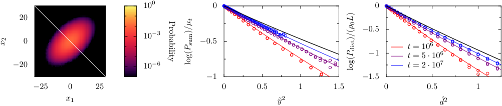
Figure 2: Large deviation functions for two TPs for ρ=0.01\rho=0.01, L=103L=10^{3} and t=106t=10^{6} Left: joint probability distribution of (x1,x2)(x_{1},x_{2}) at t=5⋅106t=5\cdot 10^{6}, the bottom-left triangle correponds to the numerical simulations while the top-right triangle is the numerical solution of (14) for two TPs (see SI). Center: rescaled marginal probability density of the half-sum Psum​((Y1+Y2)/2)P_{\mathrm{sum}}((Y_{1}+Y_{2})/2) at times t=1⋅106,5⋅106,2⋅107t=1\cdot 10^{6},5\cdot 10^{6},2\cdot 10^{7} (τ=1,5,20\tau=1,5,20). The dots are the results of numerical simulations while the colored lines comes from Eq. (15). The black curve is the prediction when τ→∞\tau\to\infty (Eq. (16)). Right: rescaled marginal probability density of the distance Pdist​((X2−X1)/2)P_{\mathrm{dist}}((X_{2}-X_{1})/2) at the same times. The black line comes from Eq. (17).

Characteristic function in the dense limit. Importantly, the characteristic function can be shown from Eq. (10) to admit the following simple form in the scaling limit t→∞t\to\infty, L=L1+⋯+LN−1→∞L=L_{1}+\dots+L_{N-1}\to\infty with fixed rescaled time τ=t/L2\tau=t/L^{2} and fixed relative lengths λi(1)=Li/L\lambda_{i}^{(1)}=L_{i}/L:

limρ0→0ψ⁡(𝐤,t)ρ0=2​tπ∑n=0N−1∑i=1N−n(cos(ki+⋯+ki+n)−1)×[g⁡(λi(n)2​τ)−g⁡(λi−1(n+1)2​τ)−g⁡(λi(n+1)2​τ)+g⁡(λi−1(n+2)2​τ)]\lim_{\rho_{0}\to 0}\frac{\psi(\mathbf{k},t)}{\rho_{0}}=\sqrt{\frac{2t}{\pi}}\sum_{n=0}^{N-1}\sum_{i=1}^{N-n}(\cos(k_{i}+\dots+k_{i+n})-1)\times\\ \bigg[g\left(\frac{\lambda_{i}^{(n)}}{\sqrt{2\tau}}\right)-g\left(\frac{\lambda_{i-1}^{(n+1)}}{\sqrt{2\tau}}\right)-g\left(\frac{\lambda_{i}^{(n+1)}}{\sqrt{2\tau}}\right)+g\left(\frac{\lambda_{i-1}^{(n+2)}}{\sqrt{2\tau}}\right)\bigg] (12)

with

g⁡(u)=e−u2−π​u​erfc​(u)g(u)=e^{-u^{2}}-\sqrt{\pi}\,u\,\text{erfc}(u) (13)

and λi(n)=(Li+⋯+Li+n−1)/L\lambda_{i}^{(n)}=(L_{i}+\dots+L_{i+n-1})/L (and λi(0)=0\lambda_{i}^{(0)}=0). We use the convention L0=LN=+∞L_{0}=L_{N}=+\infty (Fig. 1).

Equation (12) gives us the full NN-tag probability law of the SEP in the dense limit and is the main result of this Letter. In the following we analyse two important consequences.

Large deviations in the dense limit. Noticing that ψ⁡(−i​𝐬,t)=ln⁡(𝔼⁡[e𝐬⋅𝐘⁡(t)])\psi(-i\mathbf{s},t)=\ln(\mathbb{E}[e^{\mathbf{s}\cdot\mathbf{Y}(t)}]), it is possible to apply the Gärtner-Ellis theorem [29] of large deviations to get an expression for the joint probability in the large-time limit μt=ρ0​2​tπ→∞\mu_{t}=\rho_{0}\sqrt{\frac{2t}{\pi}}\to\infty:

P({y~i=μt−1Yi})\displaystyle P\left(\{\tilde{y}_{i}=\mu_{t}^{-1}Y_{i}\}\right) ≍e−μt​J​({y~i})\displaystyle\asymp e^{-\mu_{t}J(\{\tilde{y}_{i}\})} (14)

where J⁡(𝐲~)J(\mathbf{\tilde{y}}) is the Legendre transform of μt−1​ψ​(−i​𝐬)\mu_{t}^{-1}\psi(-i\mathbf{s}) and the symbol ’≍\asymp’ means equivalence at exponential order.

The probability law is best described using as variables the “half-sum of extremal displacements” Y=(Y1+YN)/2Y=(Y_{1}+Y_{N})/2 and the “distances” Di=(Yi+1−Yi)/2D_{i}=(Y_{i+1}-Y_{i})/2. For two TPs (see [22] for NN TPs), the large deviation function is found to be given by:

J(y~,d~1)=supu,v∈ℝ{uy~+vd~1−(cosh(u)−1)\displaystyle J(\tilde{y},\tilde{d}_{1})=\sup_{u,v\in\mathbb{R}}\bigg\{u\tilde{y}+v\tilde{d}_{1}-\left(\cosh(u)-1\right) (15)
−[1−g(12​τ)](2coshu2coshv2−cosh(u)−1)},\displaystyle-\left[1-g\left(\frac{1}{\sqrt{2\tau}}\right)\right]\left(2\cosh\frac{u}{2}\cosh\frac{v}{2}-\cosh(u)-1\right)\bigg\},

where y~=(y~1+y~2)/2\tilde{y}=(\tilde{y}_{1}+\tilde{y}_{2})/2 and d~1=(y~2−y~1)/2\tilde{d}_{1}=(\tilde{y}_{2}-\tilde{y}_{1})/2. This expression gives the probability law of the TPs at arbitrary times. We checked it against numerical simulations of the random walks of the vacancies and we found a very good agreement (Fig. 2).

At large rescaled time (τ→∞\tau\to\infty), it is found that

P(Y=μty~,{Di=μtd~i})\displaystyle P\left(Y=\mu_{t}\tilde{y},\{D_{i}=\mu_{t}\tilde{d}_{i}\}\right) ≍τ→∞​e−μt​I​(y~)​∏iδ⁡(d~i)\displaystyle\underset{\tau\to\infty}{\asymp}e^{-\mu_{t}I(\tilde{y})}\prod_{i}\delta(\tilde{d}_{i}) (16)
Pdist({Di=ρ0Lid^i})\displaystyle P_{\text{dist}}\left(\{D_{i}=\rho_{0}L_{i}\hat{d}_{i}\}\right) ≍τ→∞​∏ie−2​ρ0​Li​I​(d^i)\displaystyle\underset{\tau\to\infty}{\asymp}\prod_{i}e^{-2\rho_{0}L_{i}I(\hat{d}_{i})} (17)
I⁡(u)=1−1+u2\displaystyle I(u)=1-\sqrt{1+u^{2}} +u​ln⁡(u+1+u2).\displaystyle+u\ln\left(u+\sqrt{1+u^{2}}\right). (18)

In particular, we recover that all TPs behave as a single one, as shown above (see Eq. (3)). Indeed, the function II is the large deviation function involved in the dense limit of the single TP problem as can be extracted from Ref. [14] or from the limit ρ→1\rho\to 1 of Ref [15]. Note also that the marginal law of the distances PdistP_{\text{dist}} can be deduced from Eq. (2) when ρ→1\rho\to 1 in the particular case of 2 TPs [22]. Finally, at large times, in the small deviations regime, Eq. (14) gives back a Gaussian law with ⟨Y2⟩=ρ0​2​t/π\langle Y^{2}\rangle=\rho_{0}\sqrt{2t/\pi} and ⟨Di2⟩=2​ρ0​Li\langle D_{i}^{2}\rangle=2\rho_{0}L_{i}.

Universal scaling of the cumulants in the dense limit. A striking consequence of Eq. (12) is that all the even cumulants (p1+⋯+pNp_{1}+\dots+p_{N} even in Eq. (7)) are equal and assume the universal scaling form (the odd cumulants are equal to zero):

limρ0→0κeven(N)​(t)ρ0=2​tπ​g​(12​τ)+o⁡(t)\lim_{\rho_{0}\to 0}\frac{\kappa_{\text{even}}^{(N)}(t)}{\rho_{0}}=\sqrt{\frac{2t}{\pi}}g\left(\frac{1}{\sqrt{2\tau}}\right)+o(\sqrt{t}) (19)

where gg was defined in Eq. (13). Several comments are in order. (i) This expression is found to be in very good agreement with continuous-time simulations of the SEP at any time (Fig. 3). (ii) The leading order in time is the same as the one obtained for a single TP [14], as expected from Eq. (3). (iii) A major result is that the scaling form is the same for all cumulants and depends only on the distance LL between the first and the last tagged particles. (iv) The Edwards-Wilkinson equation, which is seen as the Gaussian limit of the SEP [30, 31], provides the first two cumulants and leads to κ11(2)=κ2(1)g((2τ)−1/2)\kappa^{(2)}_{11}=\kappa^{(1)}_{2}g\left((2\tau)^{-1/2}\right) at any density [32, 18] (see [22] for a numerical verification), consistently with Eq. (19). (v) A similar scaling for κ11(2)\kappa^{(2)}_{11} has also been found in the random average process [19, 20]. Note that here, this scaling form is shown to hold for all the cumulants, and for an arbitrary number of TPs.

Figure 3: Rescaled evolution of the cumulants associated to two to four TPs. ρ0=0.002\rho_{0}=0.002, L=12L=12 is the total distance. The solid colored curves correspond to the simulations in continuous time. The dashed black curve is the prediction Eq. (19).

Conclusion To sum up, we studied the joint probability distribution of an arbitrary number of tagged particles in the SEP. In the large time limit, we determined the leading behavior of all cumulants for an arbitrary density of particles. We obtained the full dynamics in the dense limit of particles and explicitly derived the time dependent large deviation function of the problem. We also unveiled a universal scaling form shared by all cumulants. We stress that this universal behavior is a non trivial high density effect. The dynamics of the cumulants for an arbitrary density of particles is expected to be non universal and remains to be determined.

References

  • [1] T. E. Harris, Journal of Applied Probability 2, 323 (1965).
  • [2] V. Gupta, S. S. Nivarthi, A. V. McCormick, and H. Ted Davis, Chemical Physics Letters 247, 596 (1995).
  • [3] K. Hahn, J. Kärger, and V. Kukla, Physical Review Letters 76, 2762 (1996).
  • [4] Wei, Bechinger, and Leiderer, Science 287, 625 (2000).
  • [5] T. Meersmann, J. W. Logan, R. Simonutti, S. Caldarelli, A. Comotti, P. Sozzani, L. G. Kaiser, and A. Pines, The Journal of Physical Chemistry A 104, 11665 (2000).
  • [6] B. Lin, M. Meron, B. Cui, S. A. Rice, and H. Diamant, Physical Review Letters 94, 216001 (2005).
  • [7] D. G. Levitt, Physical Review A 8, 3050 (1973).
  • [8] P. A. Fedders, Physical Review B 17, 40 (1978).
  • [9] S. Alexander and P. Pincus, Physical Review B 18, 2011 (1978).
  • [10] R. Arratia, The Annals of Probability 11, 362 (1983).
  • [11] L. Lizana, T. Ambjörnsson, A. Taloni, E. Barkai, and M. A. Lomholt, Physical Review E 81, 051118 (2010).
  • [12] A. Taloni and M. A. Lomholt, Physical Review E 78, 051116 (2008).
  • [13] G. Gradenigo, A. Puglisi, A. Sarracino, A. Vulpiani, and D. Villamaina, Physica Scripta 86, 058516 (2012).
  • [14] P. Illien, O. Bénichou, C. Mejía-Monasterio, G. Oshanin, and R. Voituriez, Physical Review Letters 111, 038102 (2013).
  • [15] T. Imamura, K. Mallick, and T. Sasamoto, Physical Review Letters 118, 160601 (2017).
  • [16] S. F. Burlatsky, G. Oshanin, M. Moreau, and W. P. Reinhardt, Physical Review E 54, 3165 (1996).
  • [17] C. Landim, S. Olla, and S. B. Volchan, Communications in Mathematical Physics 192, 287 (1998).
  • [18] S. Majumdar and M. Barma, Physica A: Statistical Mechanics and its Applications 177, 366 (1991).
  • [19] R. Rajesh and S. N. Majumdar, Physical Review E 64, 036103 (2001).
  • [20] J. Cividini, A. Kundu, S. N. Majumdar, and D. Mukamel, Journal of Statistical Mechanics: Theory and Experiment 2016, 053212 (2016).
  • [21] S. Sabhapandit and A. Dhar, Journal of Statistical Mechanics: Theory and Experiment 2015, P07024 (2015).
  • [22] See appendices for details of the numerical simulations and detailed calculations .
  • [23] M. J. A. M. Brummelhuis and H. J. Hilhorst, Physica A: Statistical Mechanics and its Applications 156, 575 (1989).
  • [24] O. Benichou and G. Oshanin, Phys Rev E Stat Nonlin Soft Matter Phys 66, 031101 (2002).
  • [25] O. Bénichou, A. Bodrova, D. Chakraborty, P. Illien, A. Law, C. Mejía-Monasterio, G. Oshanin, and R. Voituriez, Physical Review Letters 111, 260601 (2013).
  • [26] P. Illien, O. Bénichou, G. Oshanin, and R. Voituriez, Physical Review Letters 113, 030603 (2014).
  • [27] O. Bénichou, P. Illien, G. Oshanin, A. Sarracino, and R. Voituriez, Phys. Rev. Lett. 115, 220601 (2015).
  • [28] B. D. Hughes, Random walks and random environments, vol. 1 (Oxford University Press, 1995).
  • [29] H. Touchette, Physics Reports 478, 1 (2009).
  • [30] H. Spohn, Journal of Physics A: Mathematical and General 16, 4275 (1983).
  • [31] S. Gupta, S. N. Majumdar, C. Godrèche, and M. Barma, Physical Review E 76 (2007).
  • [32] P. L. Krapivsky, S. Redner, and E. Ben-Naim, A Kinetic View of Statistical Physics (Cambridge University Press, 2009).

Appendix A Cumulants at arbitrary density

A.1 Law of the distance between two particles

We consider two tagged particles (TPs) in the SEP with density ρ\rho. The initial distance between them is LL and we derive the equilibrium distribution of the distance (in particular we show that the distribution of the distance is time-independant at large time). We proceed as follow: (i) We write the law of the number of particles NpN_{p} between the TPs. This number is fixed initially and does not evolve. (ii) We write the law of the number of vacancies NvN_{v} between the tracers at equilibrium; this law depends on NpN_{p}.

Initially there are L−1L-1 sites between the TPs. Each site is occupied with probability ρ\rho. This gives us a binomial law for NpN_{p}:

ℙ⁡(Np=k)=(L−1k)​ρk​(1−ρ)L−1−k\mathbb{P}(N_{p}=k)=\binom{L-1}{k}\rho^{k}(1-\rho)^{L-1-k} (S20)

At large time, the number of vacancies between the two TPs, knowing that there are kk particles between them, is given by the law of the number mm of failures before k+1k+1 successes in a game in which the probability of a success is ρ\rho. It is a negative binomial law:

ℙ⁡(Nv=m|Np=k)=(m+km)​(1−ρ)m​ρk+1\mathbb{P}(N_{v}=m|N_{p}=k)=\binom{m+k}{m}(1-\rho)^{m}\rho^{k+1} (S21)

The distance DD between the tracers is given by D=Np+Nl+1D=N_{p}+N_{l}+1, its law is:

ℙ⁡(D=δ)\displaystyle\mathbb{P}(D=\delta) =∑k=0L−1ℙ⁡(Np=k)​ℙ​(Nv=δ−k−1|Np=k)\displaystyle=\sum_{k=0}^{L-1}\mathbb{P}(N_{p}=k)\mathbb{P}(N_{v}=\delta-k-1|N_{p}=k) (S22)
=∑k=0L−1(L−1k)​ρk​(1−ρ)L−1−k​(δ−1δ−k−1)​(1−ρ)δ−k−1​ρk+1\displaystyle=\sum_{k=0}^{L-1}\binom{L-1}{k}\rho^{k}(1-\rho)^{L-1-k}\binom{\delta-1}{\delta-k-1}(1-\rho)^{\delta-k-1}\rho^{k+1} (S23)
=∑k=0L−1(L−1k)​(δ−1k)​ρ2​k+1​(1−ρ)L+δ−2​k−2\displaystyle=\sum_{k=0}^{L-1}\binom{L-1}{k}\binom{\delta-1}{k}\rho^{2k+1}(1-\rho)^{L+\delta-2k-2} (S24)

This law is in very good agreement with the numerical simulations (Fig. S4).

A.2 Large deviations of the law of the distance

From the law of the distance (S24), one can derive the generating function GD​(z)G_{D}(z).

GD​(z)\displaystyle G_{D}(z) ≡∑δ=1∞ℙ⁡(D=δ)​zδ\displaystyle\equiv\sum_{\delta=1}^{\infty}\mathbb{P}(D=\delta)z^{\delta} (S25)
=∑δ=1∞zδ​∑k=0L−1ℙ⁡(Np=k)​ℙ​(Nv=δ−k−1|Np=k)\displaystyle=\sum_{\delta=1}^{\infty}z^{\delta}\sum_{k=0}^{L-1}\mathbb{P}(N_{p}=k)\mathbb{P}(N_{v}=\delta-k-1|N_{p}=k) (S26)
=z​∑k=0L−1zk​ℙ​(Np=k)​∑m=0∞zm​ℙ​(Nv=m|Np=k)\displaystyle=z\sum_{k=0}^{L-1}z^{k}\mathbb{P}(N_{p}=k)\sum_{m=0}^{\infty}z^{m}\mathbb{P}(N_{v}=m|N_{p}=k) (S27)
=z​∑k=0L−1zk​(L−1k)​ρk​(1−ρ)L−1−k​∑m=0∞(m+km)​(1−ρ)m​ρk+1\displaystyle=z\sum_{k=0}^{L-1}z^{k}\binom{L-1}{k}\rho^{k}(1-\rho)^{L-1-k}\sum_{m=0}^{\infty}\binom{m+k}{m}(1-\rho)^{m}\rho^{k+1} (S28)
=z​∑k=0L−1zk​(L−1k)​ρk​(1−ρ)L−1−k​(ρ1−(1−ρ)​z)k+1\displaystyle=z\sum_{k=0}^{L-1}z^{k}\binom{L-1}{k}\rho^{k}(1-\rho)^{L-1-k}\left(\frac{\rho}{1-(1-\rho)z}\right)^{k+1} (S29)
=(ρ​z1−(1−ρ)​z)​(ρ2​z1−(1−ρ)​z+1−ρ)L−1\displaystyle=\left(\frac{\rho z}{1-(1-\rho)z}\right)\left(\frac{\rho^{2}z}{1-(1-\rho)z}+1-\rho\right)^{L-1} (S30)

We can then derive a large deviation scaling in the limit L→∞L\to\infty:

1L​ln⁡GD​(et)→N→∞ln⁡(ρ2​z1−(1−ρ)​z+1−ρ)≡ϕ⁡(t)\frac{1}{L}\ln G_{D}(e^{t})\xrightarrow[N\to\infty]{}\ln\left(\frac{\rho^{2}z}{1-(1-\rho)z}+1-\rho\right)\equiv\phi(t) (S31)

From the Gärtner-Ellis theorem [29], this implies:

P⁡(D=L⁡(1+d~))\displaystyle P(D=L(1+\tilde{d})) ≍e−L​I​(d~)\displaystyle\asymp e^{-LI(\tilde{d})} (S32)
I⁡(d~)\displaystyle I(\tilde{d}) =supt∈ℝ​(t⁡(1+d~)−ϕ⁡(t))\displaystyle=\text{sup}_{t\in\mathbb{R}}\left(t(1+\tilde{d})-\phi(t)\right) (S33)

We now consider the high-density limit: ρ=1−ρ0\rho=1-\rho_{0} with ρ0≪1\rho_{0}\ll 1. We obtain:

ϕ(t)=t+2ρ0cosh\phi(t)=t+2\rho_{0}\cosh (S34)

Thus, the supremum in (S33) is at t∗t^{\ast} such that:

sinh⁡t∗=d~2​ρ0\sinh t^{\ast}=\frac{\tilde{d}}{2\rho_{0}} (S35)

At the end of the day,

I⁡(d~)=2​ρ0​{1−1+(d~2​ρ0)2+d~2​ρ0​log⁡(d~2​ρ0+1+(d~2​ρ0)2)}I(\tilde{d})=2\rho_{0}\left\{1-\sqrt{1+\left(\frac{\tilde{d}}{2\rho_{0}}\right)^{2}}+\frac{\tilde{d}}{2\rho_{0}}\log\left(\frac{\tilde{d}}{2\rho_{0}}+\sqrt{1+\left(\frac{\tilde{d}}{2\rho_{0}}\right)^{2}}\right)\right\} (S36)

This is exactly what is found with our high-density approach: Eq. (17) of the main text.

A.3 Large time behavior of the cumulants of NN particles

We consider NN TPs having displacements Y1,…​YNY_{1},\dots Y_{N}. We know that the moments of a single particle scale as t1/2t^{1/2} [15] while the moments of the distance scale as t0t^{0} (previous section).

⟨Y12​p⟩\displaystyle\langle Y_{1}^{2p}\rangle =𝒪⁡(t1/2)∀p∈ℕ\displaystyle=\mathcal{O}(t^{1/2})\qquad\forall p\in\mathbb{N} (S37)
⟨(Yi−Y1)2​p⟩\displaystyle\langle(Y_{i}-Y_{1})^{2p}\rangle =𝒪⁡(t0)∀i≤N,∀p∈ℕ\displaystyle=\mathcal{O}(t^{0})\qquad\forall i\leq N,\forall p\in\mathbb{N} (S38)

From this we want to show that

Ap1,…​pN(N)≡⟨Y1p1​…​YNpN⟩−⟨Y1p1+⋯+pN⟩=𝒪⁡(t1/4)∀p1,…,pNA_{p_{1},\dots p_{N}}^{(N)}\equiv\langle Y_{1}^{p_{1}}\dots Y_{N}^{p_{N}}\rangle-\langle Y_{1}^{p_{1}+\dots+p_{N}}\rangle=\mathcal{O}(t^{1/4})\qquad\forall p_{1},\dots,p_{N} (S39)

We proceed by induction: the case N=1N=1 is straightforward. Now assuming that (S39) holds for a given NN, we want to prove it for N+1N+1. As we have Ap1,…​pN,0(N+1)=Ap1,…​pN(N)=𝒪⁡(t1/4)A_{p_{1},\dots p_{N},0}^{(N+1)}=A_{p_{1},\dots p_{N}}^{(N)}=\mathcal{O}(t^{1/4}), we prove by induction that Ap1,…​pN,q(N+1)=𝒪⁡(t1/4)​∀q≥0A_{p_{1},\dots p_{N},q}^{(N+1)}=\mathcal{O}(t^{1/4})\ \forall q\geq 0. Indeed, if Ap1,…​pN,q′(N+1)=𝒪⁡(t1/4)​∀q′<qA_{p_{1},\dots p_{N},q^{\prime}}^{(N+1)}=\mathcal{O}(t^{1/4})\ \forall q^{\prime}<q, we can write:

Ap1,…​pN,q(N+1)=⟨Y1p1​…​YNpN​XN+1q⟩−⟨Y1p1+⋯+pN+q⟩\displaystyle A_{p_{1},\dots p_{N},q}^{(N+1)}=\langle Y_{1}^{p_{1}}\dots Y_{N}^{p_{N}}X_{N+1}^{q}\rangle-\langle Y_{1}^{p_{1}+\dots+p_{N}+q}\rangle (S40)
=⟨Y1p1​…​YNpN​[(YN+1−Y1)q−∑r=1q(qr)​(−1)r​Y1r​YN+1q−r]⟩−⟨Y1p1+⋯+pN+q⟩\displaystyle=\left\langle Y_{1}^{p_{1}}\dots Y_{N}^{p_{N}}\left[(Y_{N+1}-Y_{1})^{q}-\sum_{r=1}^{q}\binom{q}{r}(-1)^{r}Y_{1}^{r}Y_{N+1}^{q-r}\right]\right\rangle-\langle Y_{1}^{p_{1}+\dots+p_{N}+q}\rangle (S41)
=⟨Y1p1​…​YNpN​(YN+1−Y1)q⟩−∑r=1q(qr)​(−1)r​⟨Y1p1+r​Y2p2​…​YN+1q−r⟩−⟨Y1p1+⋯+pN+q⟩\displaystyle=\langle Y_{1}^{p_{1}}\dots Y_{N}^{p_{N}}(Y_{N+1}-Y_{1})^{q}\rangle-\sum_{r=1}^{q}\binom{q}{r}(-1)^{r}\langle Y_{1}^{p_{1}+r}Y_{2}^{p_{2}}\dots Y_{N+1}^{q-r}\rangle-\langle Y_{1}^{p_{1}+\dots+p_{N}+q}\rangle (S42)
=⟨Y1p1​…​YNpN​(YN+1−X1)q⟩−∑r=1q(qr)​(−1)r​[⟨Y1p1+r​Y2p2​…​YN+1q−r⟩−⟨Y1p1+⋯+pN+q⟩]\displaystyle=\langle Y_{1}^{p_{1}}\dots Y_{N}^{p_{N}}(Y_{N+1}-X_{1})^{q}\rangle-\sum_{r=1}^{q}\binom{q}{r}(-1)^{r}\left[\langle Y_{1}^{p_{1}+r}Y_{2}^{p_{2}}\dots Y_{N+1}^{q-r}\rangle-\langle Y_{1}^{p_{1}+\dots+p_{N}+q}\rangle\right] (S43)

All the terms in the sum are of order 𝒪⁡(t1/4)\mathcal{O}(t^{1/4}) from (S39) and the first term can be bounded by the Cauchy–Schwarz inequality:

|⟨Y1p1​…​YNpN​(YN+1−Y1)q⟩|≤⟨(Y1p1​…​YNpN)2⟩​⟨(YN+1−Y1)2​q⟩=𝒪⁡(t1/2)​𝒪​(t0)=𝒪⁡(t1/4)\left|\langle Y_{1}^{p_{1}}\dots Y_{N}^{p_{N}}(Y_{N+1}-Y_{1})^{q}\rangle\right|\leq\sqrt{\langle\left(Y_{1}^{p_{1}}\dots Y_{N}^{p_{N}}\right)^{2}\rangle\langle(Y_{N+1}-Y_{1})^{2q}\rangle}=\sqrt{\mathcal{O}(t^{1/2})\mathcal{O}(t^{0})}=\mathcal{O}(t^{1/4}) (S44)

using (S37), (S38) and (S39). This ends the proof of (S39).

This implies that if p1+⋯+pNp_{1}+\dots+p_{N} is even:

⟨Y1p1​…​YNpN⟩∼t→∞⟨Y1p1+⋯+pN⟩=𝒪⁡(t1/2)\langle Y_{1}^{p_{1}}\dots Y_{N}^{p_{N}}\rangle\mathrel{\mathop{\kern 0.0pt\sim}\limits_{t\to\infty}}\langle Y_{1}^{p_{1}+\dots+p_{N}}\rangle=\mathcal{O}(t^{1/2}) (S45)

The moments of NN particles are equal, in the large time limit, are given by the moments of a single particle. This extends to the cumulants κp1,…,pN(N)\kappa^{(N)}_{p_{1},\dots,p_{N}} defined from the second characteristic function.

ψ⁡(k1,…​kN)≡∑p1,…​pNκp1,…,pN(N)​(i​k1)p1​…​(i​kN)pNp1!​…​pN!≡log⁡[∑p1,…​pN⟨Y1p1​…​YNpN⟩​(i​k1)p1​…​(i​kN)pNp1!​…​pN!]\psi(k_{1},\dots k_{N})\equiv\sum_{p_{1},\dots p_{N}}\kappa^{(N)}_{p_{1},\dots,p_{N}}\frac{(ik_{1})^{p_{1}}\dots(ik_{N})^{p_{N}}}{p_{1}!\dots p_{N}!}\equiv\log\left[\sum_{p_{1},\dots p_{N}}\langle Y_{1}^{p_{1}}\dots Y_{N}^{p_{N}}\rangle\frac{(ik_{1})^{p_{1}}\dots(ik_{N})^{p_{N}}}{p_{1}!\dots p_{N}!}\right] (S46)
κp1,…,pN(N)∼t→∞κp1+⋯+pN(1)∼t→∞Bp1+⋯+pN​t\kappa^{(N)}_{p_{1},\dots,p_{N}}\mathrel{\mathop{\kern 0.0pt\sim}\limits_{t\to\infty}}\kappa^{(1)}_{p_{1}+\dots+p_{N}}\mathrel{\mathop{\kern 0.0pt\sim}\limits_{t\to\infty}}B_{p_{1}+\dots+p_{N}}\sqrt{t} (S47)

The coefficient BpB_{p} are computed in Ref. [15].

Figure S4: Comparison of the numerical probability distribution of the distance of two TPs (dots) with the prediction (S24) (lines) for ρ=0.25,0.5,0.75\rho=0.25,0.5,0.75 and L=5,10,20L=5,10,20. The average is performed other 10610^{6} simulations at final time t=2⋅104t=2\cdot 10^{4} (we checked that this is enough for the convergence).

Appendix B Detailed calculations in the high-density limit

B.1 Approximation and thermodynamic limit

Let us consider a system of size 𝒩\mathcal{N} with MM vacancies and denote by 𝐘⁡(t)=(Xi​(t)−Xi0)i=1N\mathbf{Y}(t)=(X_{i}(t)-X_{i}^{0})_{i=1}^{N} the vector of the displacements of the TPs. The probability P(t)​(𝐘|{Zj})P^{(t)}(\mathbf{Y}|\{Z_{j}\}) of having displacements 𝐘\mathbf{Y} at time tt knowning that the MM vacancies started at sites Z1​…​ZMZ_{1}\dots Z_{M} is exactly given by :

P(t)​(𝐘|{Zj})=∑𝐘1,…,𝐘Mδ𝐘,𝐘1+⋯+𝐘M​𝒫(t)​({𝐘j}|{Zj})P^{(t)}(\mathbf{Y}|\{Z_{j}\})=\sum_{\mathbf{Y}_{1},\dots,\mathbf{Y}_{M}}\delta_{\mathbf{Y},\mathbf{Y}_{1}+\dots+\mathbf{Y}_{M}}\mathcal{P}^{(t)}(\{\mathbf{Y}_{j}\}|\{Z_{j}\}) (S48)

where 𝒫(t)​({𝐘j}|{Zj})\mathcal{P}^{(t)}(\{\mathbf{Y}_{j}\}|\{Z_{j}\}) is the probability of displacement 𝐘j\mathbf{Y}_{j} due to the vacancy jj for all jj knowing the initial positions of all the vacancies.

Assuming that in the large density large (ρ→1\rho\to 1) the vacancies interact independantly with the TPs, we can link it to the probability pZ(t)​(𝐘)p^{(t)}_{Z}(\mathbf{Y}) that the tracers have moved by 𝐘\mathbf{Y} at time tt due to a single vacancy that was initially at site ZZ:

𝒫(t)​({𝐘j}|{Zj})​∼ρ→1​∏j=1MpZj(t)​(𝐘j)\mathcal{P}^{(t)}(\{\mathbf{Y}_{j}\}|\{Z_{j}\})\underset{\rho\to 1}{\sim}\prod_{j=1}^{M}p^{(t)}_{Z_{j}}(\mathbf{Y}_{j}) (S49)

so that

P(t)​(𝐘|{Zj})​∼ρ→1​∑𝐘1,…,𝐘Mδ𝐘,𝐘1+⋯+𝐘M​∏j=1MpZj(t)​(𝐘j)P^{(t)}(\mathbf{Y}|\{Z_{j}\})\underset{\rho\to 1}{\sim}\sum_{\mathbf{Y}_{1},\dots,\mathbf{Y}_{M}}\delta_{\mathbf{Y},\mathbf{Y}_{1}+\dots+\mathbf{Y}_{M}}\prod_{j=1}^{M}p^{(t)}_{Z_{j}}(\mathbf{Y}_{j}) (S50)

We take the Fourier transform and we average over the initial positions of the vacancies:

p~(t)​(𝐤)≡1𝒩−N​∑Z∉{Xi0}∑𝐘pZ(t)​(𝐘)​ei​𝐤𝐘\tilde{p}^{(t)}(\mathbf{k})\equiv\frac{1}{\mathcal{N}-N}\sum_{Z\notin\{X_{i}^{0}\}}\sum_{\mathbf{Y}}p^{(t)}_{Z}(\mathbf{Y})e^{i\mathbf{k}\mathbf{Y}} (S51)

and mutatis mutandis for P~(t)​(𝐤)\tilde{P}^{(t)}(\mathbf{k}). Furthermore we write p~Z(t)​(𝐤)=1+q~Z(t)​(𝐤)\tilde{p}_{Z}^{(t)}(\mathbf{k})=1+\tilde{q}_{Z}^{(t)}(\mathbf{k}) (qZq_{Z} corresponds to the deviation from a Dirac centered in 00).

P~(t)​(𝐤)​∼ρ→1​[p~(t)​(𝐤)]M=[1𝒩−N​∑Z∉{Xi0}p~Z(t)​(𝐤)]M=[1+1𝒩−N​∑Z∉{Xi0}q~Z(t)​(𝐤)]M\tilde{P}^{(t)}(\mathbf{k})\underset{\rho\to 1}{\sim}\left[\tilde{p}^{(t)}(\mathbf{k})\right]^{M}=\left[\frac{1}{\mathcal{N}-N}\sum_{Z\notin\{X_{i}^{0}\}}\tilde{p}_{Z}^{(t)}(\mathbf{k})\right]^{M}=\left[1+\frac{1}{\mathcal{N}-N}\sum_{Z\notin\{X_{i}^{0}\}}\tilde{q}_{Z}^{(t)}(\mathbf{k})\right]^{M} (S52)

We now take the limit 𝒩,M→∞\mathcal{N},M\to\infty with ρ0≡1−ρ=M/𝒩\rho_{0}\equiv 1-\rho=M/\mathcal{N} (density of vacancies) remaining constant. The second characteristic function reads:

limρ0→0ψ(t)​(𝐤)ρ0≡limρ0→0ln⁡[P~(t)​(𝐤)]ρ0=∑Z∉{Xi0}q~Z(t)​(𝐤)\lim_{\rho_{0}\to 0}\frac{\psi^{(t)}(\mathbf{k})}{\rho_{0}}\equiv\lim_{\rho_{0}\to 0}\frac{\ln\left[\tilde{P}^{(t)}(\mathbf{k})\right]}{\rho_{0}}=\sum_{Z\notin\{X_{i}^{0}\}}\tilde{q}_{Z}^{(t)}(\mathbf{k}) (S53)

B.2 Expression of the single-vacancy propagator

One can partition over the first passage of the vacancy to the site of one of the tracers to get an expression for q~Z\tilde{q}_{Z} which is the main quantity involved in (S53):

pZ(t)​(𝐘)\displaystyle p_{Z}^{(t)}(\mathbf{Y}) =δ𝐘,𝟎​(1−∑j=0t∑ν=±1,±2Fν,Z(j))+∑j=0t∑ν=±1,±2p−ν(t−j)​(𝐘)​Fν,Z(j)\displaystyle=\delta_{\mathbf{Y},\mathbf{0}}\left(1-\sum_{j=0}^{t}\sum_{\nu=\pm 1,\pm 2}F^{(j)}_{\nu,Z}\right)+\sum_{j=0}^{t}\sum_{\nu=\pm 1,\pm 2}p_{-\nu}^{(t-j)}(\mathbf{Y})F^{(j)}_{\nu,Z} (S54)
p~Z(t)​(𝐤)\displaystyle\tilde{p}_{Z}^{(t)}(\mathbf{k}) =1−∑j=0t∑ν=±1,±2Fν,Z(j)+∑j=0t∑ν=±1,±2p~−ν(t−j),ζ​(𝐤)​Fν,Z(j)\displaystyle=1-\sum_{j=0}^{t}\sum_{\nu=\pm 1,\pm 2}F^{(j)}_{\nu,Z}+\sum_{j=0}^{t}\sum_{\nu=\pm 1,\pm 2}\tilde{p}_{-\nu}^{(t-j),\zeta}(\mathbf{k})F^{(j)}_{\nu,Z} (S55)
q~Z(t)​(𝐤)\displaystyle\tilde{q}_{Z}^{(t)}(\mathbf{k}) =−∑j=0t∑ν=±1,±2[1−(1+q~−ν(t−j),ζ(𝐤))Fν,Z(j)]\displaystyle=-\sum_{j=0}^{t}\sum_{\nu=\pm 1,\pm 2}\left[1-\left(1+\tilde{q}_{-\nu}^{(t-j),\zeta}(\mathbf{k})\right)F^{(j)}_{\nu,Z}\right] (S56)

An exponant ζ\zeta to a quantity means that this quantity is computed taking into account ζ=ζ⁡(Z)\zeta=\zeta(Z).

We now need an expression for q~ηζ\tilde{q}_{\eta}^{\zeta} where η\eta is a special site. To do so we decompose the propagator of the displacements over the successive passages of the vacancy to the position of one of the tracers:

pη(t),ζ​(𝐘)=δ𝐘,𝟎​(1−∑j=0t∑μFμ,η(j),ζ)+∑p=1∞∑m1,…,mp=1∞∑mp+1=0∞δt,∑imi∑ν1,…,νpδ𝐘,∑i𝐞νi(1−∑j=0mp+1∑μF(j),ζμ,−νp)F(mp),ζνp,−νp−1…F(m2),ζν2,−ν1F(m1),ζν1,ηp^{(t),\zeta}_{\eta}(\mathbf{Y})=\delta_{\mathbf{Y},\mathbf{0}}\left(1-\sum_{j=0}^{t}\sum_{\mu}F^{(j),\zeta}_{\mu,\eta}\right)\\ +\sum_{p=1}^{\infty}\sum_{m_{1},\dots,m_{p}=1}^{\infty}\sum_{m_{p+1}=0}^{\infty}\delta_{t,\sum_{i}\!m_{i}}\sum_{\nu_{1},\dots,\nu_{p}}\delta_{\mathbf{Y},\sum_{i}\!\mathbf{e}_{\nu_{i}}}\left(1-\sum_{j=0}^{m_{p+1}}\sum_{\mu}F^{(j),\zeta}_{\mu,-\nu_{p}}\right)F^{(m_{p}),\zeta}_{\nu_{p},-\nu_{p-1}}\dots F^{(m_{2}),\zeta}_{\nu_{2},-\nu_{1}}F^{(m_{1}),\zeta}_{\nu_{1},\eta} (S57)

the sums on μ\mu and νi\nu_{i} run over the special sites (±1,⋯±N\pm 1,\dots\pm N).

The discrete Laplace transform (power series) of a function of time g⁡(t)g(t) is g^​(ξ)≡∑t=0∞g⁡(t)​ξt\hat{g}(\xi)\equiv\sum_{t=0}^{\infty}g(t)\xi^{t}. We can now take both the Laplace and Fourier transforms of (S57) to get:

p^ηζ​(𝐘,ξ)=11−ξ​{δ𝐘,𝟎​(1−∑μF^μ,νζ)+∑p=1∞∑ν1,…,νpδ𝐘,∑i𝐞νi​∑μ(1−F^μ,−νpζ)​F^νp,−νp−1ζ​…​F^ν2,−ν1ζ​F^ν1,ηζ}\hat{p}_{\eta}^{\zeta}(\mathbf{Y},\xi)=\frac{1}{1-\xi}\left\{\delta_{\mathbf{Y},\mathbf{0}}\left(1-\sum_{\mu}\hat{F}_{\mu,\nu}^{\zeta}\right)+\sum_{p=1}^{\infty}\sum_{\nu_{1},\dots,\nu_{p}}\delta_{\mathbf{Y},\sum_{i}\!\mathbf{e}_{\nu_{i}}}\sum_{\mu}\left(1-\hat{F}_{\mu,-\nu_{p}}^{\zeta}\right)\hat{F}_{\nu_{p},-\nu_{p-1}}^{\zeta}\dots\hat{F}_{\nu_{2},-\nu_{1}}^{\zeta}\hat{F}_{\nu_{1},\eta}^{\zeta}\right\} (S58)
q~^ηζ​(𝐤,ξ)≡p~^ηζ​(𝐤,ξ)−11−ξ=11−ξ​∑μ,ν{[1−Tζ​(𝐤,ξ)]−1}ν​μ×(1−e−i​𝐤𝐞ν)​ei​𝐤𝐞μ​F^μ​ηζ​(ξ)\hat{\tilde{q}}_{\eta}^{\zeta}(\mathbf{k},\xi)\equiv\hat{\tilde{p}}_{\eta}^{\zeta}(\mathbf{k},\xi)-\frac{1}{1-\xi}=\frac{1}{1-\xi}\sum_{\mu,\nu}\{[1-T^{\zeta}(\mathbf{k},\xi)]^{-1}\}_{\nu\mu}\times\left(1-e^{-i\,\mathbf{k}\mathbf{e}_{\nu}}\right)e^{i\,\mathbf{k}\mathbf{e}_{\mu}}\hat{F}^{\zeta}_{\mu\eta}(\xi) (S59)

The matrix TT is defined by Tζ​(𝐤,ξ)ν​μ=F^ν,−μζ​(ξ)​ei​𝐤𝐞νT^{\zeta}(\mathbf{k},\xi)_{\nu\mu}=\hat{F}^{\zeta}_{\nu,-\mu}(\xi)e^{i\,\mathbf{k}\mathbf{e}_{\nu}}.

B.3 Expression of the characteristic function

Introducing (S56) into (S53) directly gives:

limρ0→0ψ^​(𝐤,ξ)ρ0\displaystyle\lim_{\rho_{0}\to 0}\frac{\hat{\psi}(\mathbf{k},\xi)}{\rho_{0}} =−∑ν[11−ξ−(11−ξ+q~^−ν(ζ)(𝐤,ξ))ei​𝐤𝐞ν]hζ(ξ)\displaystyle=-\sum_{\nu}\bigg[\frac{1}{1-\xi}-\left(\frac{1}{1-\xi}+\hat{\tilde{q}}^{(\zeta)}_{-\nu}(\mathbf{k},\xi)\right)e^{i\,\mathbf{k}\mathbf{e}_{\nu}}\bigg]h_{\zeta}(\xi) (S60)
hζ​(ξ)\displaystyle h_{\zeta}(\xi) =∑Z∉{Xi0}F^ζ,Z​(ξ)=∑Z=Xζ0+1Xζ+10−1F^ζ,Z​(ξ)\displaystyle=\sum_{Z\notin\{X_{i}^{0}\}}\hat{F}_{\zeta,Z}(\xi)=\sum_{Z=X_{\zeta}^{0}+1}^{X_{\zeta+1}^{0}-1}\hat{F}_{\zeta,Z}(\xi) (S61)

with q~^νζ\hat{\tilde{q}}_{\nu}^{\zeta} given by (S59).

B.4 Expression of the quantities of interest (F^ν,η(ζ)\hat{F}_{\nu,\eta}^{(\zeta)} and hμh_{\mu})

The two results [28] that we recalled in the article are:

  • •

    The Laplace transform of the first passage density at the origin at time tt of a symmetric 1d Polya walk starting from site ll is:

    f^l​(ξ)=α|l|​ with ​α=1−1−ξ2ξ\hat{f}_{l}(\xi)=\alpha^{|l|}\mbox{ with }\alpha=\frac{1-\sqrt{1-\xi^{2}}}{\xi} (S62)
  • •

    The probability of first passage at site s1s_{1} starting from s0s_{0} and considering s2s_{2} as an absorbing site is given by

    F^†​(s1|s0,ξ)=f^s1−s0​(ξ)−f^s1−s2​(ξ)​f^s2−s0​(ξ)1−f^s1−s2​(ξ)2\hat{F}^{\dagger}(s_{1}|s_{0},\xi)=\frac{\hat{f}_{s_{1}-s_{0}}(\xi)-\hat{f}_{s_{1}-s_{2}}(\xi)\hat{f}_{s_{2}-s_{0}}(\xi)}{1-\hat{f}_{s_{1}-s_{2}}(\xi)^{2}} (S63)

From (S62), we have:

F^−1,−1=F^+N,+N=α\hat{F}_{-1,-1}=\hat{F}_{+N,+N}=\alpha (S64)

From (S62, S63), and recalling that the distance between TP μ\mu and TP μ+1\mu+1 is Lμ(ζ)L_{\mu}^{(\zeta)}, we have

F^μ,μ(ζ)=F^−μ+1,−μ−1(ζ)\displaystyle\hat{F}_{\mu,\mu}^{(\zeta)}=\hat{F}_{-\mu+1,-\mu-1}^{(\zeta)} =α−α2​Lμ(ζ)−11−α2​Lμ(ζ)\displaystyle=\frac{\alpha-\alpha^{2L_{\mu}^{(\zeta)}-1}}{1-\alpha^{2L_{\mu}^{(\zeta)}}} (S65)
F^μ,−μ+1(ζ)=F^−μ+1,μ(ζ)\displaystyle\hat{F}_{\mu,-\mu+1}^{(\zeta)}=\hat{F}_{-\mu+1,\mu}^{(\zeta)} =αLμ(ζ)−1−αLμ(ζ)+11−α2​Lμ(ζ)\displaystyle=\frac{\alpha^{L_{\mu}^{(\zeta)}-1}-\alpha^{L_{\mu}^{(\zeta)}+1}}{1-\alpha^{2L_{\mu}^{(\zeta)}}} (S66)

And the sums are:

h0=hN\displaystyle h_{0}=h_{N} =∑Z=−∞−1α|Z|=α1−α\displaystyle=\sum_{Z=-\infty}^{-1}\alpha^{|Z|}=\frac{\alpha}{1-\alpha} (S67)
hμ\displaystyle h_{\mu} =∑Z=1Lμ−1α−α2​Lμ−Z1−α2​Lμ=α⁡(1−αLμ−1)​(1−αLμ)(1−α)​(1−α2​Lμ)\displaystyle=\sum_{Z=1}^{L_{\mu}-1}\frac{\alpha-\alpha^{2L_{\mu}-Z}}{1-\alpha^{2L_{\mu}}}=\frac{\alpha(1-\alpha^{L_{\mu}-1})(1-\alpha^{L_{\mu}})}{(1-\alpha)(1-\alpha^{2L_{\mu}})} (S68)

Appendix C Results in the high density limit

C.1 Scaling of the characteristic function

Using a numerical software (Mathematica) we obtain the following result for the discrete Laplace tranform of the second characteristic function is:

limρ0→0ψ^​(𝐤,ξ)ρ0=1(1−α2)​(1−ξ)∑n=0N−1∑i=1N−nαℒin{2α(1−αLi−1)(1−αLi+n)cos(ki+⋯+ki+n)+(1−α)Qn(ki,…,ki+n)+C}\lim_{\rho_{0}\to 0}\frac{\hat{\psi}(\mathbf{k},\xi)}{\rho_{0}}=\frac{1}{(1-\alpha^{2})(1-\xi)}\sum_{n=0}^{N-1}\sum_{i=1}^{N-n}\alpha^{\mathcal{L}_{i}^{n}}\bigg\{2\alpha(1-\alpha^{L_{i-1}})(1-\alpha^{L_{i+n}})\cos(k_{i}+\dots+k_{i+n})\\ +(1-\alpha)Q_{n}(k_{i},\dots,k_{i+n})+C\bigg\} (S69)

with CC a constant enforcing ψ^​(𝐤=𝟎)=0\hat{\psi}(\mathbf{k}=\mathbf{0})=0 and

ℒin\displaystyle\mathcal{L}_{i}^{n} =Li+⋯+Li+n−1\displaystyle=L_{i}+\dots+L_{i+n-1} (S70)
Q2​(k1,k2)\displaystyle Q_{2}(k_{1},k_{2}) =αL1​(ei​k1+e−i​k2)\displaystyle=\alpha^{L_{1}}\left(e^{ik_{1}}+e^{-ik_{2}}\right) (S71)
Q3​(k1,k2,k3)\displaystyle Q_{3}(k_{1},k_{2},k_{3}) =αL1(ei​k1+e−i​k2)+αL2(ei​k2+e−i​k3)+αL1+L2(ei⁡(k1+k2)+e−i⁡(k2+k3)+2cosk2)\displaystyle=\alpha^{L_{1}}\left(e^{ik_{1}}+e^{-ik_{2}}\right)+\alpha^{L_{2}}\left(e^{ik_{2}}+e^{-ik_{3}}\right)+\alpha^{L_{1}+L_{2}}\left(e^{i(k_{1}+k_{2})}+e^{-i(k_{2}+k_{3})}+2\cos k_{2}\right) (S72)

Similar expressions exist for Qn,n>3Q_{n},n>3.

We define the total length L=L1+⋯+LN−1L=L_{1}+\dots+L_{N-1} and the rescaled variables lin=ℒin/Ll_{i}^{n}=\mathcal{L}_{i}^{n}/L.

We define p=1−ξp=1-\xi and p~=p​L2\tilde{p}=pL^{2}. We take the limit L→∞L\to\infty keeping p~\tilde{p} constant. This is a limit of large time.

The asymptotic behavior of α\alpha is given by :

α=1−1−ξ2ξ=1−2​p+𝒪p→0​(p)\alpha=\frac{1-\sqrt{1-\xi^{2}}}{\xi}=1-\sqrt{2p}+\mathcal{O}_{p\to 0}(p) (S73)

so that

αr​L​∼L→∞​e−r​2​p~\alpha^{rL}\underset{L\to\infty}{\sim}e^{-r\sqrt{2\tilde{p}}} (S74)

(S69) becomes :

limρ0→0ψ^​(𝐤,p=L2​p~)ρ0​∼L→∞​L32​p~3/2​∑n=0N−1∑i=1N−n(e−2​p~​lin−e−2​p~​li−1n+1−e−2​p~​lin+1+e−2​p~​li−1n+2)×(cos⁡(ki+⋯+ki+n)−1)\lim_{\rho_{0}\to 0}\frac{\hat{\psi}(\mathbf{k},p=L^{2}\tilde{p})}{\rho_{0}}\underset{L\to\infty}{\sim}\frac{L^{3}}{\sqrt{2}\tilde{p}^{3/2}}\sum_{n=0}^{N-1}\sum_{i=1}^{N-n}\left(e^{-\sqrt{2\tilde{p}}\,l_{i}^{n}}-e^{-\sqrt{2\tilde{p}}\,l_{i-1}^{n+1}}-e^{-\sqrt{2\tilde{p}}\,l_{i}^{n+1}}+e^{-\sqrt{2\tilde{p}}\,l_{i-1}^{n+2}}\right)\\ \times\left(\cos(k_{i}+\dots+k_{i+n})-1\right) (S75)

The following continuous inverse Laplace tranform is known:

h^​(p)=e−r​2​pp3/2⇔h⁡(t)=2​tπ​g​(r2​t)\hat{h}(p)=\frac{e^{-r\sqrt{2p}}}{p^{3/2}}\Leftrightarrow h(t)=2\sqrt{\frac{t}{\pi}}g\left(\frac{r}{\sqrt{2t}}\right) (S76)
g⁡(u)=e−u2−π​u​erfc⁡(u)g(u)=e^{-u^{2}}-\sqrt{\pi}\,u\,\erfc(u) (S77)

(S75) can then be inverted and we find:

limρ0→0ψ⁡(𝐤,t)ρ0​∼t→∞​2​tπ​∑n=0N−1∑i=1N−n[g⁡(Lin2​t)−g⁡(Li−1n+12​t)−g⁡(Lin+12​t)+g⁡(Li−1n+22​t)]×(cos⁡(ki+⋯+ki+n)−1)\lim_{\rho_{0}\to 0}\frac{\psi(\mathbf{k},t)}{\rho_{0}}\underset{t\to\infty}{\sim}\sqrt{\frac{2t}{\pi}}\sum_{n=0}^{N-1}\sum_{i=1}^{N-n}\left[g\left(\frac{L_{i}^{n}}{\sqrt{2t}}\right)-g\left(\frac{L_{i-1}^{n+1}}{\sqrt{2t}}\right)-g\left(\frac{L_{i}^{n+1}}{\sqrt{2t}}\right)+g\left(\frac{L_{i-1}^{n+2}}{\sqrt{2t}}\right)\right]\\ \times\left(\cos(k_{i}+\dots+k_{i+n})-1\right) (S78)

C.2 Effects of the initial conditions on the odd cumulants

We consider two TPs at an initial distance LL. We show that, due to the fact that we impose their initial positions, the two TPs separate slightly from one another.

From (S69) and (S71) we obtain:

limρ0→0⟨X2⟩​(ξ)ρ0=αL(1+α)​(1−ξ)∼L→∞L2​e−2​p~2​p~\lim_{\rho_{0}\to 0}\frac{\langle X_{2}\rangle(\xi)}{\rho_{0}}=\frac{\alpha^{L}}{(1+\alpha)(1-\xi)}\mathrel{\mathop{\kern 0.0pt\sim}\limits_{L\to\infty}}L^{2}\frac{e^{-\sqrt{2\tilde{p}}}}{2\tilde{p}} (S79)

with p~=(1−ξ)/L2\tilde{p}=(1-\xi)/L^{2}.

The inversion of the Laplace transform gives:

limρ0→0⟨X2⟩​(t)ρ0∼t→∞12​erfc​(L2​t)\lim_{\rho_{0}\to 0}\frac{\langle X_{2}\rangle(t)}{\rho_{0}}\mathrel{\mathop{\kern 0.0pt\sim}\limits_{t\to\infty}}\frac{1}{2}\text{erfc}\left(\frac{L}{\sqrt{2t}}\right) (S80)

and similarly

limρ0→0⟨X1⟩​(t)ρ0∼t→∞−12​erfc​(L2​t)\lim_{\rho_{0}\to 0}\frac{\langle X_{1}\rangle(t)}{\rho_{0}}\mathrel{\mathop{\kern 0.0pt\sim}\limits_{t\to\infty}}-\frac{1}{2}\text{erfc}\left(\frac{L}{\sqrt{2t}}\right) (S81)

We indeed see that the two tracers separate a little bit. This effect is obvious when L=1L=1: initially the two TPs are on neighboring sites, and at large time there is a probability ρ0\rho_{0} that there is a vacancy inbetween: ⟨X2−X2⟩​(t→∞)=ρ0\langle X_{2}-X_{2}\rangle(t\to\infty)=\rho_{0}.

Similar effects are expected on all the odd cumulants in the NN-tag problem. These effect also add a term of order t0t^{0} in the even cumulants.

C.3 Large deviation function for a single TP

For a single tracer at high density our approach (which coincides with [14]) gives:

ψ⁡(k,t)=μt​(cos⁡k−1)\psi(k,t)=\mu_{t}\left(\cos k-1\right) (S82)

with μt=ρ0​2​tπ\mu_{t}=\rho_{0}\sqrt{\frac{2t}{\pi}}. The Gärtner-Ellis theorem gives:

P⁡(Yi=μt​y~)\displaystyle P\left(Y_{i}=\mu_{t}\tilde{y}\right) ≍e−μt​I​(y~)\displaystyle\asymp e^{-\mu_{t}I(\tilde{y})} (S83)
I⁡(y~)\displaystyle I(\tilde{y}) =supq∈ℝ(q​y~−(cosh⁡q−1))\displaystyle=\sup_{q\in\mathbb{R}}\left(q\tilde{y}-(\cosh q-1)\right) (S84)

Solving for the extremum gives:

e±q=±y~+1+y~2e^{\pm q}=\pm\tilde{y}+\sqrt{1+\tilde{y}^{2}} (S85)

and finally:

I⁡(y~)=1−1+y~2+y~​ln⁡[y~+1+y~2]I(\tilde{y})=1-\sqrt{1+\tilde{y}^{2}}+\tilde{y}\ln\left[\tilde{y}+\sqrt{1+\tilde{y}^{2}}\right] (S86)

C.4 Large deviation function for NN TPs

We assume that the limits ρ0→0\rho_{0}\to 0 and t→∞t\to\infty can be exchanged (this would need to be proven) and we write

ψ⁡(i​𝐪,t)​∼ρ0→0t→∞​μt​∑n=0N−1∑i=1N−n[g⁡(Λinπ)−g⁡(Λi−1n+1π)−g⁡(Λin+1π)+g⁡(Λi−1n+2π)]×(cosh⁡(qi+⋯+qi+n)−1)\psi(i\mathbf{q},t)\underset{\begin{subarray}{c}\rho_{0}\to 0\\ t\to\infty\end{subarray}}{\sim}\mu_{t}\sum_{n=0}^{N-1}\sum_{i=1}^{N-n}\left[g\left(\frac{\Lambda_{i}^{n}}{\sqrt{\pi}}\right)-g\left(\frac{\Lambda_{i-1}^{n+1}}{\sqrt{\pi}}\right)-g\left(\frac{\Lambda_{i}^{n+1}}{\sqrt{\pi}}\right)+g\left(\frac{\Lambda_{i-1}^{n+2}}{\sqrt{\pi}}\right)\right]\\ \times\left(\cosh(q_{i}+\dots+q_{i+n})-1\right) (S87)

with μt=ρ0​2​tπ\mu_{t}=\rho_{0}\sqrt{\frac{2t}{\pi}} and Λin=Lin​π2​t\Lambda_{i}^{n}=L_{i}^{n}\sqrt{\frac{\pi}{2t}}. In the following, the limits will be implicit.

The Gärtner-Ellis theorem [29] for μt→∞\mu_{t}\to\infty then gives us the probability distribution (at exponential order, denoted ≍\asymp).

P({Yi=μty~i})\displaystyle P\left(\{Y_{i}=\mu_{t}\tilde{y}_{i}\}\right) ≍e−μt​J​({y~i})\displaystyle\asymp e^{-\mu_{t}J(\{\tilde{y}_{i}\})} (S88)
J⁡({y~i})\displaystyle J(\{\tilde{y}_{i}\}) =sup{qi}∈ℝ(∑i=1Nqi​y~i−μt−1​ψ​(−i​𝐪))\displaystyle=\sup_{\{q_{i}\}\in\mathbb{R}}\left(\sum_{i=1}^{N}q_{i}\tilde{y}_{i}-\mu_{t}^{-1}\psi(-i\mathbf{q})\right) (S89)

To simplify the problem we define the following variables:

Y=Y1+YN2Di=Yi+1−Yi2(i=1,…​N−1)Y=\frac{Y_{1}+Y_{N}}{2}\qquad D_{i}=\frac{Y_{i+1}-Y_{i}}{2}\quad(i=1,\dots N-1) (S90)
u=q1+⋯+qNvi=−q1−⋯−qi+qi+1+⋯+qN(i=1,…​N−1)u=q_{1}+\dots+q_{N}\qquad v_{i}=-q_{1}-\dots-q_{i}+q_{i+1}+\dots+q_{N}\quad(i=1,\dots N-1) (S91)

Small rescaled length.

g⁡(Λ/π)=1−Λ+𝒪Λ→0​(Λ2)g(\Lambda/\sqrt{\pi})=1-\Lambda+\mathcal{O}_{\Lambda\to 0}(\Lambda^{2}) (S92)

At the first order in the rescaled lengths, only the “boundary” terms contribute in (S87). Using the variables defined above, one checks that (S89) becomes simpler:

J⁡(y~,{d~i})​∼Λi≪1​supu,{vi}∈ℝ{u​y~+∑i=1N−1vi​d~i−(cosh⁡(u)−1)−∑i=1N−1Λi​(2​cosh⁡u2​cosh⁡vi2−cosh⁡(u)−1)}J(\tilde{y},\{\tilde{d}_{i}\})\underset{\Lambda_{i}\ll 1}{\sim}\sup_{u,\{v_{i}\}\in\mathbb{R}}\bigg\{u\tilde{y}+\sum_{i=1}^{N-1}v_{i}\tilde{d}_{i}-\left(\cosh(u)-1\right)-\sum_{i=1}^{N-1}\Lambda_{i}\left(2\cosh\frac{u}{2}\cosh\frac{v_{i}}{2}-\cosh(u)-1\right)\bigg\} (S93)

This extremum can only be solved for in the special cases defined in the main text: Λi=0\Lambda_{i}=0, marginal probability of the distances (this corresponds to u=0u=0) and Gaussian limit (y~≪1\tilde{y}\ll 1, v~i≪1\tilde{v}_{i}\ll 1).

Two tracers, arbitrary length. One should note that for two tracers, (S89) is already rather simple if written with the right variables: we don’t need to assume Λ≪1\Lambda\ll 1.

J⁡(y~,d~)=supu,v∈ℝ{u​y~+v​d~−(cosh⁡(u)−1)−(1−g⁡(Λπ))​(2​cosh⁡u2​cosh⁡v2−cosh⁡(u)−1)}J(\tilde{y},\tilde{d})=\sup_{u,v\in\mathbb{R}}\bigg\{u\tilde{y}+v\tilde{d}-\left(\cosh(u)-1\right)-\left(1-g\left(\frac{\Lambda}{\sqrt{\pi}}\right)\right)\left(2\cosh\frac{u}{2}\cosh\frac{v}{2}-\cosh(u)-1\right)\bigg\} (S94)

This expression is used to provide a numerical predition in the main text.

C.5 Numerical verification of the expression of κ11(2)\kappa^{(2)}_{11} at arbitrary density

From the Edwards-Wilkinson equation, one expects :

κ11(2)=κ2(1)​g​(12​τ)=1−ρρ​2​tπ​g​(12​τ)\kappa^{(2)}_{11}=\kappa^{(1)}_{2}g\left(\frac{1}{\sqrt{2\tau}}\right)=\frac{1-\rho}{\rho}\sqrt{\frac{2t}{\pi}}g\left(\frac{1}{\sqrt{2\tau}}\right) (S95)

This behavior is in good agreement with numerical simulations (see Fig. S5, left).

For the other cumulants, we showed that

limt→∞κp1,…,pN(N)t=limt→∞κp1+⋯+pN(1)t=Bp1+⋯+pN,\lim_{t\to\infty}\frac{\kappa^{(N)}_{p_{1},\dots,p_{N}}}{\sqrt{t}}=\lim_{t\to\infty}\frac{\kappa^{(1)}_{p_{1}+\dots+p_{N}}}{\sqrt{t}}=B_{p_{1}+\dots+p_{N}}, (S96)

where the constants BkB_{k} characteristic of a single tracer have been determined in Ref. [15].

Figure S5: Evolution of the cumulants associated to two TPs at different densities and different distances. The cumulants are rescaled by the single-tag cumulants, following (S95). The dashed line corresponds to g((2τ)−1/2)g((2\tau)^{-1/2}).

C.6 Argument for the breaking of our scaling shape at arbitrary density

In analogy with (S95), one would like to be able to make the following bold conjecture :

κp,2​n−p(2)=B2​ntg((2τ)−1/2)\kappa^{(2)}_{p,2n-p}=B_{2n}\sqrt{t}\,g\left((2\tau)^{-1/2}\right)

Unfortunately we show that this is incompatible with the law of the distance (S24).

Let us focus on the 4th cumulant of the distance (we denote ⟨⟩c\langle\rangle_{c} the cumulants) :

⟨(X2−X1)4⟩c=⟨X14⟩c+⟨X24⟩c−4​⟨X13​X2⟩c−4​⟨X1​X23⟩c+6​⟨X12​X22⟩c\langle(X_{2}-X_{1})^{4}\rangle_{c}=\langle X_{1}^{4}\rangle_{c}+\langle X_{2}^{4}\rangle_{c}-4\langle X_{1}^{3}X_{2}\rangle_{c}-4\langle X_{1}X_{2}^{3}\rangle_{c}+6\langle X_{1}^{2}X_{2}^{2}\rangle_{c} (S97)

We assume that :

⟨X14⟩c=⟨X24⟩c\displaystyle\langle X_{1}^{4}\rangle_{c}=\langle X_{2}^{4}\rangle_{c} =B4​t+o⁡(1)\displaystyle=B_{4}\sqrt{t}+o(1) (S98)
⟨X13​X2⟩c=⟨X1​X23⟩c=⟨X12​X22⟩c\displaystyle\langle X_{1}^{3}X_{2}\rangle_{c}=\langle X_{1}X_{2}^{3}\rangle_{c}=\langle X_{1}^{2}X_{2}^{2}\rangle_{c} =B4​t​g​(12​τ)=B4​t−B4​π2​L+o⁡(1)\displaystyle=B_{4}\sqrt{t}g\left(\frac{1}{\sqrt{2\tau}}\right)=B_{4}\sqrt{t}-B_{4}\sqrt{\frac{\pi}{2}}L+o(1) (S99)

This leads us to:

⟨(X2−X1)4⟩c=2​π​B4​L\langle(X_{2}-X_{1})^{4}\rangle_{c}=\sqrt{2\pi}B_{4}L (S100)

From Ref. [15],

B4=2π​1−ρρ3​[1−(4−(8−3​2)​ρ)​(1−ρ)+12π​(1−ρ)2]B_{4}=\sqrt{\frac{2}{\pi}}\frac{1-\rho}{\rho^{3}}\left[1-(4-(8-3\sqrt{2})\rho)(1-\rho)+\frac{12}{\pi}(1-\rho)^{2}\right] (S101)

while from (S24),

⟨(X2−X1)4⟩c∼L→∞2​L​1−ρρ3​(12−24​ρ+13​ρ2)\langle(X_{2}-X_{1})^{4}\rangle_{c}\mathrel{\mathop{\kern 0.0pt\sim}\limits_{L\to\infty}}2L\frac{1-\rho}{\rho^{3}}\left(12-24\rho+13\rho^{2}\right) (S102)

At an arbitrary density, this is inconsistent with (S100), thus our conjecture must be wrong. Note that (S100) does hold as expected when ρ→1\rho\to 1.

In Fig. S5 center (resp. right), we tried the following guess: κ222=B4tg((2τ)−1/2)\kappa^{2}_{22}=B_{4}\sqrt{t}\,g\left((2\tau)^{-1/2}\right) (resp. κ312=B4tg((2τ)−1/2)\kappa^{2}_{31}=B_{4}\sqrt{t}\,g\left((2\tau)^{-1/2}\right)). We see that it is valid only at high density, as expected.

Appendix D Description of numerical simulations

D.1 Continuous time simulations on a lattice (for the cumulants)

NpartsN_{\text{parts}} particles are put uniformly at random on the line of size NsizeN_{\text{size}}, except the NN tagged particles which are put deterministically on their initial positions. We used Nsize=5000N_{\text{size}}=5000

Each particle has an exponential clock of time constant τ=1\tau=1. Thus, the whole system has an exponential clock of time constant τall=τ/Nparts\tau_{\text{all}}=\tau/N_{\text{parts}}. When it ticks, a particle is chosen at random and tries to move either to the left or to the right with probability 1/21/2. If the arrival site is already occupied the particle stays where it was.

The cumulants of the NN TPs are averaged over 100 000 to 500 000 simulations to obtain their time dependence.

D.2 Vacancy-based simulations (for the probability distribution)

The previous approach does not enable one to get sufficient statistics to investigate the probability law.

In the case of ponctual brownian particles, Ref. [21] was able to use the propagator of the displacement to directly obtain the state of the system at a given time and investigate the probability distribution.

Here we used a numerical scheme close to out theoretical approach: at high density and in discrete time, we simulate the behavior of the vacancies considered as independant random walker. The displacement Δ​x\Delta x of a vacancy at (discrete) time tt is given by a binomial law:

Δ​x\displaystyle\Delta x =2​nright−t\displaystyle=2n_{\text{right}}-t (S103)
P⁡(nright,t)\displaystyle P(n_{\text{right}},t) =12t​(tnright)\displaystyle=\frac{1}{2^{t}}\binom{t}{n_{\text{right}}} (S104)

One is able to recover the final positions of the TPs from the final positions of the vacancies.

For two TPs at distance LL, we put a vacancy at each site between the TPs with probability ρ0\rho_{0} (density of vacancies). We consider a number of sites NsitesN_{\text{sites}} (Nsites=100 000N_{\text{sites}}=100\,000) on the left of the first TP and on the right of the second TP and we put a deterministic number of vacancies Nvac=ρ0​NsitesN_{\text{vac}}=\rho_{0}N_{\text{sites}} at random positions on these sites.

We make 10810^{8} repetition of the simulation before outputting the probability law.