Gradient-based dimension reduction of multivariate vector-valued functions Thanks: Submitted to the editors on 20 October 2018.
Abstract
Multivariate functions encountered in high-dimensional uncertainty quantification problems often vary along a few dominant directions in the input parameter space. We propose a gradient-based method for detecting these directions and using them to construct ridge approximations of such functions, in a setting where the functions are vector-valued (e.g., taking values in ). The methodology consists of minimizing an upper bound on the approximation error, obtained by subspace Poincaré inequalities. We provide a thorough mathematical analysis in the case where the parameter space is equipped with a Gaussian probability measure. The resulting method generalizes the notion of active subspaces associated with scalar-valued functions. A numerical illustration shows that using gradients of the function yields effective dimension reduction. We also show how the choice of norm on the codomain of the function has an impact on the function’s low-dimensional approximation.
keywords
High-dimensional function approximation, dimension reduction, active subspace, ridge approximation, Karhunen-Loève decomposition, Poincaré inequality, Sobol’ indices.AMS
41A30, 41A63, 65D151 Introduction
Many problems that arise in uncertainty quantification—e.g., integrating or approximating multivariate functions—suffer from the curse of dimensionality: the complexity of algorithms grows dramatically (typically exponentially) with the dimension of the input parameter space. One approach to alleviate this curse is to identify and exploit some notion of low-dimensional structure. For example, the function of interest might vary primarily along a few directions of the input parameter space while being (almost) constant in the other directions. In this case, we say that the problem has a low intrinsic dimension; algorithms for quantifying uncertainty can then focus on these important directions to reduce the overall cost.
A common and simple approach for parameter space dimension reduction is the truncated Karhunen-Loève decomposition [50], closely related to principal component analysis [27]. These techniques exploit the correlation structure of the function’s input space (specifically, decay in the spectrum of the covariance of the input measure). However, more effective dimension reduction is possible with techniques that exploit not only input correlations but also the structure of the input-output map itself. One way to reduce the input space dimension is to determine the non-influential input parameters (or factors) and to fix them to some arbitrary value. Factor fixing (see, e.g., [47]) is often a goal of global sensitivity analysis [46, 24]. For independent inputs, total Sobol’ indices [47] are a popular way to address the factor fixing problem, as they measure the total impact that each variable (or each group of variables) has on the variance of the output. Estimating these indices can be computationally challenging, however; see for instance [51, 22, 52]. Alternative screening procedures based on derivative-based global sensitivity measures (DGSM) have been proposed in [29, 28]. These indices are defined as integrals of squared derivatives of the model output. If the numerical implementation of a model permits easy computation of the derivatives (for instance using the adjoint method, see [43]), these indices can be estimated with reasonable computational cost. There are interesting links between DGSM and Sobol’ indices. For instance, assuming the inputs are independent, one can bound the total Sobol’ indices by the DGSM up to some Poincaré constant that depends on the probability distribution of the parameters (see, e.g., [29, 31] and [44] for a recent detailed analysis). Yet the factor fixing setting is somewhat restrictive, in that functions often vary most prominently in directions that are not aligned with the coordinate axes corresponding to the original inputs.
Closely related to derivative-based screening are active subspaces, described in [45, 7, 10]. Active subspaces are defined as the leading eigenspaces of the second moment matrix of the function’s gradient, the diagonal of which contains the DGSM. These eigenspaces are not necessarily aligned with the canonical coordinates, and hence are able to identify linear combinations of the input parameters along which the function varies the most. In this sense, they generalize coordinate-aligned derivative-based global sensitivity analysis. Active subspaces have been used in a wide range of science and engineering models [36, 9, 25]. Connections between Sobol’ indices, DGSM, and active subspaces for scalar-valued functions are explored in [8].
Global sensitivity analysis and active subspaces have primarily been focused on scalar-valued functions, as in models with a single output quantity of interest. In the presence of multiple outputs of interest, as is the case in many practical applications, new approaches are needed. Aggregated Sobol’ indices for multiple outputs or functional outputs have been introduced in [32], and further studied in [18, 19]. In the context of active subspaces, one could try to identify important input parameter directions for each output and then combine all those directions, as in [26]. But it is not clear how to interpret or even best perform such a combination step.
1.1 Contribution
In this paper, we propose a methodology for detecting and exploiting the low intrinsic dimension that a given multivariate function might have. We formulate our approach as a controlled approximation problem, seeking a certified upper bound for the error in a ridge approximation of the original function. With this approximation perspective, our methodology extends naturally to the case of vector-valued functions—for instance, functions with multiple real-valued outputs. Specifically, given a function of interest
where is a vector space, the problem is to find an approximation of by a function of fewer variables, say with where depends linearly on . Thus, given a user-defined tolerance , we seek a linear function such that
| (1) |
holds for some function , where is a norm chosen depending on the application. Approximations of the form of are called ridge functions [42]. If such an approximation exists with , we say that has a low effective dimension , and correspond to the active (or explanatory) variables. To solve this controlled approximation problem, we use Poincaré-type inequalities to derive an upper bound on the error. This bound, defined by means of gradients (or Jacobians) of , admits a simple expression and can be analytically minimized with respect to and for any fixed . By choosing such that the minimized error bound is below the prescribed tolerance , we obtain an approximation of whose error is controlled. We also show that, for scalar-valued functions , the minimizer of the bound corresponds to the active subspace approach proposed in [10].
In our analysis we assume that the parameter domain is equipped with a Gaussian probability measure, and we define the norm in (1) as the corresponding weighted norm. Thus (1) becomes an approximation problem for in the mean-squared sense. The Gaussian measure need not be standard: it can have non-zero mean and non-identity covariance matrix. By allowing the latter, we will show that the notion of a low effective dimension also depends on the input covariance matrix itself. Furthermore, having non-standard Gaussian measures enables us to compare our approach with the truncated Karhunen-Loève decomposition, which also exploits the spectral properties of the parameter covariance matrix. The Gaussian assumption primarily permits us to simplify our analysis. One can consider other probability measures as long as they satisfy the so-called subspace Poincaré inequality described later in the paper, which is the key argument of our method. Explicit generalizations of this inequality to non-Gaussian measures are given in [53].
It is important to mention that in actual practice, minimizing the error itself is a much more difficult problem than minimizing the error bound. This is why the proposed strategy is appealing, provided that gradient information from is available. However, there is no guarantee that the minimizer of the bound is close to the minimizer of the true error. To illustrate the potential and the limitations of the proposed method, we present (in Section 5.1) examples of functions for which minimizing the bound gives either the minimizer of the error (ideal case) or the maximizer of the error (worst case). In both cases the proposed method still permits us to control the approximation error: it simply does so more efficiently in the first case than in the second. We also demonstrate our method on a parameterized partial differential equation (see Section 5.2). This example shows that the resulting ridge approximation depends not only on but also on the choice of norm on the output space , which in turn defines the function-space norm in (1).
Ridge functions and their approximation properties were extensively studied in the 1980s because of their connection to both projection pursuit regression [17, 13, 23] and early neural networks [21]. Recent work has exploited compressed sensing to recover a ridge function from point queries [15, 6]. The ridge recovery problem corresponds to the proposed problem setup (1) with : the goal is to recover , , and assuming that is exactly a ridge function . In contrast, we do not aim for an exact recovery of , but rather approximation of by a ridge function up to a prescribed precision . Similar recovery problems arise in the statistical regression literature under the name sufficient dimension reduction [1, 12]. In this context, the goal is to identify linear combinations in the input space that are statistically sufficient to explain the regression response. Among the numerous sufficient dimension reduction techniques that have been proposed, we mention sliced inverse regression [33], sliced average variance estimation [11], and principal Hessian directions [34]. In [48], gradient information is used to explore the underlying regression structure by means of average derivative functionals, estimated nonparametrically via kernels. Concerning dimension reduction in regression with vector-valued responses, a broad literature has also emerged more recently. We refer to [54] and references therein (see also [35, 49, 2]). Broadly, and in contrast with the approach proposed here, these regression analyses are concerned with estimation from a given data set, and thus rely on statistical assessments of the error.
The rest of this paper is organized as follows. Section 2 describes our dimension reduction methodology, deriving an upper bound on the error and an explicit construction for its minimizer, yielding a controlled ridge approximation of a vector-valued function. Section 3 compares the proposed method with the truncated Karhunen-Loève decomposition, and Section 4 discusses its relationship with sensitivity analysis. In Section 5 we demonstrate our method on various analytical and numerical examples. Proofs of the main results are deferred to Appendix A.
2 Dimension reduction of the input parameter space
Throughout the paper, the algebraic space refers to a parameter space of dimension . The Borel sets of are denoted by and we let be the Gaussian probability measure on with mean and covariance , which is assumed to be non-singular. We let be an algebraic space endowed with a norm associated with a scalar product defined by for any , where is a symmetric positive definite matrix. We denote by
the Hilbert space which contains all the measurable functions such that , where is the norm associated with the scalar product defined by
for any .
Ridge functions are functions of the form where is a linear function and where is a measurable function, sometimes called the profile of the ridge function; see [38]. Ridge functions are essentially functions that are constant along a subspace (the kernel of ). In this paper we will use the following parametrization of ridge functions,
| (2) |
where is a rank- projector and is a measurable function. Notice that whenever , which means that the function (2) is constant along the kernel of the projector, and thus is a ridge function.11 1 One can easily show that any function as in (2) can be written as for some linear and some measurable , and vice versa.
We consider the problem of finding a controlled approximation of a function by a ridge function. Given a prescribed tolerance , the problem consists in finding and such that
| (3) |
The choice (the identity matrix) and in (2) yields a trivial solution. But in that case, the rank of is equal to and there is no dimension reduction. Thus, in order to make this problem meaningful, we want to be less than , ideally .
Remark 1.
An equivalent formulation of the problem is the following. Given a tolerance , we want to find a Borel function and a low-rank projector such that
where is a random vector and where denotes the mathematical expectation. If , the statistical interpretation is that the random variable is an explanatory variable for , in the sense that most of the variance of can be explained by .
2.1 Optimal profile for the ridge function
In this section, we assume that the projector is given. We denote by
the space containing all the -measurable functions such that . Here is the -algebra generated by . By the Doob–Dynkin lemma, see for example Lemma 1.13 in [39], the set of all -measurable functions is exactly the set of the functions of the form for some Borel function , so that
| (4) |
Note that is a closed subspace in . Then, for any , there exists a unique minimizer of over . This minimizer corresponds to the orthogonal projection of onto and is denoted by . We can write
which means that yields an optimal profile . Note that can be uniquely characterized by the variational equation
| (5) |
for all . In other words, corresponds to the conditional expectation of under the distribution given the -algebra , which explains the choice of notation. The following proposition gives an interesting property on the space . The proof is given in Appendix A.1.
Proposition 2.
Let and be two projectors such that . Then we have
Let us recall that a projector is uniquely characterized by both its kernel and its image.22 2 Of course an orthogonal projector (orthogonal with respect to any scalar product) is uniquely characterized either by its kernel or by its image, since the other subspace can be uniquely defined as the orthogonal complement. Proposition 2 shows that is invariant with respect to the image of , and so is the conditional expectation . In particular, the error depends only on the kernel of . This means that, with regard to the initial dimension reduction problem (3), the goal is now to find a subspace where the function does not vary.
By Proposition 2 and without loss of generality, we can assume that is an orthogonal projector with respect to an arbitrary scalar product on . In the present context, the natural scalar product to use is the one induced by the precision matrix of , which is for any . The associated norm is such that for any . The projector is -orthogonal if for all , which is equivalent to
| (6) |
for all . The following proposition gives a simple expression for the conditional expectation , provided satisfies (6). The proof is given in Appendix A.2.
Proposition 3.
Let where is a non-singular covariance matrix and . Then for any -orthogonal projector we have
where the expectation is taken over the random vector .
2.2 Poincaré-based upper bound for the error
In this section we show how Poincaré-type inequalities can be used to derive an upper bound for the error. This upper bound holds for any projector and is quadratic in so that it can easily be minimized.
It is well known that the standard Gaussian distribution satisfies the Poincaré inequality
| (7) |
for any continuously differentiable function , where denotes the gradient of (see for example Theorem 3.20 in [3]). Here and denotes the canonical norm of . As noticed in [5], non-standard Gaussian distributions also satisfy a Poincaré inequality. By replacing by in (7), where is a symmetric square root of , we have that satisfies
| (8) |
for any continuously differentiable function , where is the norm on such that for all . The next proposition shows that satisfies another Poincaré-type inequality which we call the subspace Poincaré inequality. The proof is given in Appendix A.3.
Proposition 4.
The probability distribution satisfies
| (9) |
for any continuously differentiable function and for any projector .
The subspace Poincaré inequality stated in Proposition 4 allows us to derive an upper bound for the error , as shown by the following proposition, whose proof is given in Appendix A.4.
Proposition 5.
Let , where is a non-singular covariance matrix, and let , where is endowed with a norm such that for some symmetric positive definite matrix . Furthermore, assume that is continuously differentiable. Then for any projector we have
| (10) |
where is the matrix defined by
| (11) |
Here, denotes the Jacobian matrix of at point given by
| (12) |
Note that the matrix defined in (11) depends not only on but also on the norm of the output space via the matrix .
2.3 Minimizing the upper bound
The following proposition enables minimization of the upper bound in Proposition 5. The proof is given in Appendix A.5.
Proposition 6.
Let be a symmetric positive-definite matrix and a symmetric positive-semidefinite matrix. Denote by the -th generalized eigenpair of the matrix pair , meaning with . For any we have
| (13) |
Furthermore a solution to the above minimization problem is the -orthogonal projector defined by
| (14) |
By Propositions 5 and 6 we have that, for a sufficiently regular function , the error can be controlled by means of the generalized eigenvalues of the matrix pair as follows
where is the projector defined as in (14) and as in (11). The matrix pair provides a test to reveal the low intrinsic dimension of the function . Indeed, a fast decay in the spectrum of ensures that goes quickly to zero with . In that case, given , there exists and a projector with rank such that . Notice, however, that a fast decay in the spectrum of is only a sufficient condition for the low intrinsic dimension: the absence of decay in the does not mean that cannot be well approximated by for some low-rank projector .
3 Contrast with the truncated Karhunen-Loève decomposition
A simple yet powerful dimension reduction method is the truncated Karhunen-Loève (K-L) decomposition. Truncated K-L decompositions are widely used in forward UQ—for instance, in any parameterized elliptic PDE where one truncates the K-L representation of the stochastic process modeling the uncertain parameters, and computes the resulting PDE solution; see, e.g., [4, 16, 40]. The goal of this section is to position the method we proposed in Section 2 against truncation of the K-L decomposition of the input parameters to . In particular, under a Lipschitz continuity assumption on , we show that K-L truncation can also be seen as a function approximation technique that minimizes an upper bound. We then show that this upper bound is looser than the bound we derived using Poincaré inequalities.
The truncated K-L decomposition consists in reducing the parameter space to the subspace spanned by the leading eigenvectors of the covariance matrix of . This approach is based on the observation that
| (15) |
where and where is the -th eigenvalue of . We recall that denotes the canonical norm of . If the left-hand side of (15) is small, then the random variable can be well approximated (in the sense) by , where is a solution33 3 Consider the eigendecomposition of . Then the projector is a solution to (15). to (15). In that case, given a function , we can hope that is a good approximation of . In order to make a quantitative statement, we assume is Lipschitz continuous, meaning that there exists a constant such that
| (16) |
for all . Letting , we can write
| (17) |
If the eigenvalues of decay rapidly, then there exist a function and a projector such that , where . In other words, the low intrinsic dimension of a Lipschitz continuous function can be revealed by the spectrum of . Approximations that exploit this type of low-dimensional structure have been used extensively in forward and inverse uncertainty quantification; see, e.g., [37].
Notice that the function considered here does not satisfy in general, and therefore is not the optimal choice of profile; see Section 2.1.
Proposition 7.
Let be a continuously differentiable function and let be a minimizer of , where and where is the covariance matrix of . If is Lipschitz continuous such that (16) holds for some , we have
where and are the -th eigenvalues of and of the matrix pair respectively.
The proof is given in Appendix A.6. Similar to the methodology proposed in this paper, the truncated K-L decomposition can be interpreted as a method that minimizes an upper bound of an approximation error; see equation (17). Proposition 7 shows that the minimum of the upper bound of the new method is always smaller or equal to that of the truncated K-L. Of course comparing upper bounds does not allow one to make any clear statement about which method performs better than the other. However, note that for the truncated K-L decomposition, the construction of the projector relies only on the covariance matrix , whereas the proposed method also takes into account the function (through the matrix ) in the construction of . Thus it is natural to expect the new approach to provide projectors that are better for the approximation of .
4 Connection with global sensitivity measures
The goal of global sensitivity analysis is to assign, to each group of input variables, a value that reflects its contribution to the variance of the output. When considering a scalar-valued function with , classical variance-based indices include the closed Sobol’ indices and the total Sobol’ indices, defined respectively as:
| (18) |
Here and represent components of the random vector indexed by and , where is a set of indices with and where is its complement in . For independent inputs (e.g., diagonal ), the closed index measures ’s contribution to the output variance. The total index measures the contribution of and its interactions, of any order and with any other input variables, to the output variance.
The definitions in (18) do not apply to vector-valued functions. A natural extension of these indices is to interpret the variance of a (scalar-valued) function as an norm, e.g., where with . With this perspective, a natural extension of Sobol’ indices to the vector-valued case is
| (19) |
Note that the definitions in (18) and (19) are equivalent for scalar-valued functions. We mention that a similar44 4 To be specific, the generalization proposed in [18, 19] is , where and , where is a given matrix. One can easily show that if , which means for any , then this definition matches the one proposed in (19). generalization of the Sobol’ index has been proposed in [18, 19]. Using standard properties of the conditional expectation, one can rewrite the above indices as
and
where is the projector such that (resp. ) extracts the coordinates of indexed by (resp. by ). As noticed in [20], the above expressions allow for an interpretation of the Sobol’ indices with an approximation perspective. On the one hand, quantifies how well a function can be approximated by , a function which depends only on the -coordinates of the parameter (large means we should not remove the dependence). On the other hand, quantifies how good an approximation of can be if we remove the coordinates indexed by (small means we can remove the dependence).
A straightforward application of Proposition 5 allows us to bound the indices and as follows:
| (20) |
and
| (21) |
where . In the scalar-valued case, coincides with the th derivative-based global sensitivity measure (DGSM) [29, 28]. The fact that the DGSM can bound the total Sobol’ index has been already noted [29, 30, 31, 44] for scalar-valued functions, and for more general input distributions than Gaussian ones. Here, under the assumption of Gaussian probability measure , inequality (21) provides a generalization of these bounds to the case of vector-valued functions, where the th DGSM ought to be defined as . The same remark applies for inequality (20).
5 Illustrations
5.1 Analytical examples
We give here three analytical examples for which we can compute a closed-form expression for the error . This allows us to find the projector that minimizes the true error. We then compare this projector with the one that minimizes the upper bound of .
First we consider a linear function. We show that the bound equals the true error, so that minimizing the bound gives the minimizer of the error itself. Then we consider a quadratic function: in this case, the bound is not equal to the error, but the minimizers are the same. Finally we consider a function defined as a sum of sine functions. Depending on the frequency and amplitude of the sines, minimizing the bound can either yield the optimal projector (minimizer of the error) or the worst projector (maximizer of the error)! This last example offers some useful intuition, showing that the proposed method performs better for slowly varying functions than for functions of small amplitude but high frequency.
5.1.1 Linear functions
Assume is a linear function for some matrix and let be a -orthogonal projector. By Proposition 3 and by linearity of we have for any . We can write
where, for the last equality, we used the relations and . Thus we have that equality is attained in (10) for any linear functions and for any -orthogonal projector . This shows that, for linear functions, the upper bound is equal to the true error.
5.1.2 Quadratic forms
Assume is the standard normal distribution and let be a quadratic form defined by for some symmetric matrix . It is a real-valued function so that and , the absolute value. Let be an orthogonal projector with rank so that . One can easily check that the relation
holds for all where . By taking the expectation with respect to , Proposition 3 allows writing The function is quadratic and can be written as where and . We have
Consider the eigendecomposition of and let . We have so that
where denotes the Frobenius norm. One can show that the rank- projector which minimizes is the projector onto the leading eigenspace of . Denoting by the -th largest eigenvalue of , we have
| (22) |
Now we consider the projector that minimizes the upper bound given by Proposition 5. We can write so that . Therefore equation (10) yields
for any orthogonal projector with rank . By Proposition 6, the rank- orthogonal projector which minimizes the right-hand side in the above inequality is the projector onto the leading eigenspace of , which is the same as the solution to (22). Then the minimizer of the bound is, for the considered example, the same as the minimizer of the error itself. In addition, the upper bound evaluated at the optimal projector allows controlling the error by which is, up to a factor of , the same as the true error.
5.1.3 Sum of sines
Let be a standard normal distribution. Consider the real-valued function such that
for any , where and are two vectors. Let be an orthogonal projector. For simplicity, we restrict our analysis to the case where is a projector onto the span of vectors from the canonical basis of , meaning
| (23) |
where and . It is readily seen that is the function . We can show that
where is the complementary set of in and . Therefore, the projector of the form of (23) which minimizes the error is the one associated with the set containing the indices of the largest values of .
Now we find the projector of the form (23) that minimizes the upper bound of the error given by Proposition 5. Recall that , so we can write
The projector (23) that minimizes the above upper bound is the one associated with the set containing the indices of the largest values of . We now describe two interesting cases.
- •
Assume that all the frequencies are the same, for all . The index sets corresponding to the largest and are the same, and therefore the projector that minimizes the upper bound is the same as the minimizer of the true error. Notice, however, that when the true error tends to , whereas the upper bound tends to infinity. This shows that the upper bound can be a poor estimator for the error, even if its minimization allows recovery of the optimal projector.
- •
Suppose now that for all . Then the index set corresponding to the largest is the same as the index set of the smallest . Indeed is increasing on whereas is decreasing. Hence, for this particular example, minimizing the upper bound yields the worst possible projector, i.e., the one that maximizes the true error.
These two cases show the limitations of the use of Poincaré inequalities: the bound is not sharp for functions with small variation but high frequencies. However, it works well for slowly varying functions. The same remark applies directly to sensitivity analysis (see Section 4): the DGSM should not be used to bound the Sobol’ indices unless the function varies slowly with respect to its input parameters.
5.2 Elliptic PDE
Consider the diffusion equation on the square domain , which consists in finding in the Sobolev space such that
| (24) |
Here denotes the spatial coordinates and refers to the gradient in the spatial variable . The diffusion coefficient is a random field and follows a log-normal distribution such that is a Gaussian process on with zero mean and with a covariance function defined by for all . A numerical approximation of (24) is obtained with the finite element method (FEM); see, for example, [14]. The diffusion field is approximated by the piecewise constant random field
| (25) |
where denotes the indicator function associated with the th element of the mesh represented in Figure 1(a). Here corresponds to the number of elements, and with
and being the center of the th element. With a slight abuse of notation, we denote by the Galerkin projection of the solution to (24) onto the space of continuous piecewise affine functions associated with the mesh in Figure 1(a). We consider the following scenarios, where the function is defined by three different post-solution treatments of :
- 1.
, which means that is the solution map from the parameter to the FEM solution to (24). In that case is the FEM approximation space with dimension , the number of nodes in the mesh. Since , the natural choice for the norm is
- 2.
, where . In other words, corresponds to the restriction of to a subdomain of . For this scenario, is of dimension (the number of nodes in ) and is endowed with the norm given by
- 3.
, where and . In this scenario, we are interested in the evaluation of the solution at two different spatial locations and . There are two scalar-valued outputs so that is an algebraic space. Consider the weighted norm defined by
where are two positive weights to be specified. For example the choice will put twice the weight on the error associated with the first output compared to the second. This is a way to model the fact that, for the final purpose of the simulation, one output is more important than the other.
Remark 8.
Each of the three functions defined above are continuously differentiable, as a composition of continuously differentiable functions. Indeed, we can write each with some matrix which depends on the scenario and where and are the FEM matrix and FEM right-hand side associated with (24). Because of the parameterization (25) of the diffusion field , the function is continuously differentiable so that is also continuously differentiable, and so is .
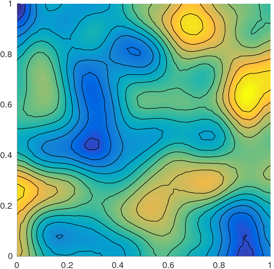

| Scenario 1 | Scenario 2 | Scenario 3 | ||
|---|---|---|---|---|

|

|
|||
5.2.1 Computational aspects
We consider the problem of computing the matrix . Since , with , can be approximated by the -sample Monte Carlo estimate
| (26) |
where are independent copies of . To numerically compute a realization of , one needs to evaluate the Jacobian of the function times. To do so, we employ the adjoint method; see for example [43]. Then, to construct the projector, instead of minimizing we consider a projector such that
| (27) |
By construction, depends upon , and thus it is random. Recall that such a projector can be obtained by computing the generalized eigendecomposition of the matrix pair ; see Proposition 6.
To approximate the conditional expectation , we consider the random function
| (28) |
where are independent copies of . Given a realization of the projector , a realization of can be obtained by drawing samples of and by using those samples to evaluate using (28). Notice that the samples are not redrawn for each new evaluation point of . By Proposition 3 and for any , can be interpreted as an -sample Monte Carlo approximation of . Finally, notice that if and (i.e., the mean of ), then our approximation of reduces to the form used in Section 3 when truncating a K-L decomposition, albeit for a different projector; see relation (17) with and .
5.2.2 Modes and influence of the norm
For each scenario, an approximation of is computed with a large number of samples, . This approximation is considered sufficiently accurate and will be used in place of . Figure 2 illustrates the leading generalized eigenvectors of the matrix pair as well as the leading eigenvectors of , meaning the K-L modes; see Section 3. Since they do not depend upon , the K-L modes do not have any particular relation to the elliptic PDE solution other than some symmetry properties related to the shape of the domain . In contrast, the modes associated with the three scenarios present specific features which depend on the function . For example with scenario 2, we observe that the modes in the parameter space somehow represent more information local to the region of interest .
The choice of the norm also impacts the generalized eigenvectors of through the matrix . For instance with scenario 3 we have allows us to write
With the choice , the modes in Figure 2 suggest that the two points of interest and are considered equally important, whereas the choice and leads to significantly more patterns around point (on the top-left of ) than around point .
| mode 1 | mode 2 | mode 3 | mode 4 | mode 5 | mode 6 | |
|---|---|---|---|---|---|---|
|
K-L |
 |
 |
 |
 |
 |
 |
|
Scenario 1 |
 |
 |
 |
 |
 |
 |
|
Scenario 2 |
 |
 |
 |
 |
 |
 |
|
|
 |
 |
 |
 |
 |
 |
|
|
 |
 |
 |
 |
 |
 |
5.2.3 Approximating the conditional expectation and comparison with K-L
Assume the matrix is known (again, a sufficiently accurate approximation with samples is used in place of ) and let be the rank- projector which minimizes . We consider the approximation of the conditional expectation given by (28) with . Figure 3 shows the error as a function of the rank of the projector. For each scenario, one realization of is computed with either , , or samples. We first note that, since we do not exactly compute the conditional expectation, the errors (dotted curves) are sometimes above the upper bound (solid red curves). In this inexact setting, is no longer a certified upper bound for the error. However we observe it can still be used as a good error indicator.
The three scenarios do not have the same convergence rate with : the first scenario has the slowest and the third the fastest. Even though they are different post-solution treatments of the same solution map , the functions associated with each scenario do not have the same complexity in terms of intrinsic dimension.
Interestingly, increasing does not lead to significant improvements of the approximation. This phenomenon can be explained by the following relation,
where the expectation is taken over the samples (the projector being fixed here). This result shows that even with small , one can still hope to obtain a good approximation of provided is chosen such that is sufficiently small. In other words a crude approximation of the conditional expectation yields at most a factor of two (when ) in the expected error squared, so that it remains of the same order of magnitude as ; see also Theorem 3.2 from [10].
We now compare with the truncated Karhunen-Loève decomposition, for which is defined as the rank- orthogonal projector onto the leading eigenspace of the covariance matrix . The black dash-dotted curves in Figure 3 represent the upper bound for this choice of , as a function of . (The true error is substantively the same as its upper bound, so we decided not to plot it.) It is interesting to see that in the first scenario, the K-L projector is essentially as effective as the projector obtained by minimizing the upper bound. As shown in Figure 4, the spectrum of is flat, which means that is close to a rescaled identity matrix. Then, minimizing is nearly the same as minimizing , where , and yields the same projector as the truncated K-L method; see (15). However, this reasoning does not apply to scenarios 2 and 3, where the spectrum of decays rapidly. For these scenarios we observe in Figure 3 that the new method outperforms the truncated K-L method. For instance, in scenario 2 the new method reaches an error of with only whereas the truncated K-L method requires .
5.2.4 Quality of the projector
In this section we assess the quality of a projector defined by (27), where is the -sample Monte Carlo approximation of given by (26). In the present context, an optimal projector would be a minimizer of so that the only relevant criteria for the quality of is how close is to the minimum of the upper bound. Figure 5 contains two sets of curves: the solid curves represent the error bound as a function of the rank of , whereas the dotted curves correspond to the approximate error bound . This approximate error bound is the quantity we would use in place of the error bound when the matrix is not known. For each scenario we observe that for small , the approximate error bound underestimates the true error bound. This means that can be used as an error estimator only if is sufficient large.
Observe in Figure 5 that scenarios 1 and 2 need fewer samples to obtain a good projector (say around samples) compared to the last scenario (at least samples). To understand this result, let us note that if is larger than the rank of , the projector is not uniquely determined: any such that is a solution to (27). Therefore the rank of should not exceed that of which, thanks to (26), satisfies the following relation
With scenario 3 we have so that the rank of should not exceed . This limitation is represented by the vertical lines on Figure 5(c). With scenarios 1 and 2 we have and so that this limit is not attained within the range of the plots. The conclusion is that when the dimension of is large, one needs fewer samples from to obtain a suitable projector, because each sample is a matrix with potentially a large rank.
6 Conclusions
We have addressed the problem of approximating multivariate functions taking values in a vector space. We approximate such functions by means of ridge functions that depend on a number of linear combinations of the input parameters that is smaller than the original dimension. Rather than seeking an optimal approximation, we build a controlled approximation: we develop an upper bound on the approximation error and minimize this upper bound.
Our analytical and numerical examples demonstrate good performance of the method, and also illustrate conditions under which it might not work well. For example, we show cases where minimizing the upper bound leads to an optimal approximation, and contrasting cases where the error bound is not tight. Numerical demonstrations on an elliptic PDE also illustrate various computational issues: sampling to compute both the projector (yielding the important directions) and the conditional expectation (yielding the ridge profile).
Future work may explore several natural extensions of the proposed methodology. First is the extension to non-Gaussian input measures, e.g., uniform measure on bounded domains in . Second is the extension to infinite-dimensional input spaces: for example, letting the domain of be a function space endowed with Gaussian or Besov measure. Finally, it may be possible to develop sharper error bounds based on higher-order derivatives, e.g., Hessians of . For the last two points, we may be able to use recent results on higher-order Poincaré inequalities [41].
Appendix A Proofs
A.1 Proof of Proposition 2
Let . By (4) we can write for some Borel function . Since we have for all . Also for any we have and then . Thus holds for any so that . Then which shows that . Then the inclusion holds. By symmetry of the role of and we obtain the result.
A.2 Proof of Proposition 3
Let and . By (4), can be written as for some Borel function so that for all . We can write
where the expectation is taken over the random vector , where and are two independent random vectors distributed as . If then the previous relation yields (5) for any , which would conclude the proof.
It remains to show that . Note that is Gaussian with mean and covariance
Then if and only if . Since is -orthogonal, relation (6) holds for any which is equivalent to
Multiplying by to the left (resp. by to the right) we get (resp. ) so that the relation holds and yields . Therefore we have
which concludes the proof.
A.3 Proof of Proposition 4
First we assume that is a -orthogonal projector. Let be a continuously differentiable function and define for some . For any we have . By Proposition 3 we have
Notice that we can write . Then the Poincaré inequality (8) applied with the function yields
Recall that, since is -orthogonal, we have whenever and are independent; see the proof of Proposition 3. Thus, replacing by in the previous inequality and taking the expectation over yields (9).
It remains to show that (9) also holds for projectors that are not -orthogonal. Thus let be any projector and define as the (unique) -orthogonal projector such that . Following the proof of Proposition 3, we have that satisfies which is equivalent to saying that the relation holds for any . Then for any . Replacing by we get
| (29) |
For the last equality we used relation , which holds true since . Finally, Proposition 2 allows writing so that
which shows that (9) holds for any projector .
A.4 Proof of Proposition 5
Denote by the -th eigenpair of the matrix so that and for any . The function can be represented as where . The linearity of the conditional expectation permits to write
| (30) |
Because is continuously differentiable, the coordinate are continuously differentiable as well. Then the subspace Poincaré inequality (9) yields
By definition of the Jacobian matrix (12) we have . Then, together with (30), the above relation yields
where for the last equality we used the relation and the definition (11) of . This concludes the proof.
A.5 Proof of Proposition 6
Let and be symmetric square roots of and respectively. For any projector we have
where and and where denotes the Frobenius norm. Consider the singular value decomposition of where are two orthogonal matrices and with . The Eckart-Young theorem states that (i) the matrix , with , is a minimizer of over all matrices with and (ii) that . We now show that can be written as for some rank- projector . Let be the matrix containing the first columns of and let . Since we have so that is a rank- projector. Also we have . Then holds for any rank- matrix , in particular for the ones of the form of for any rank- projector . This shows that the minimum in (13) is reached by . Furthermore it is easy to check that holds so that, as we saw in the proof of Proposition 3, is -orthogonal.
It remains to show that can be written as in (14). Notice that holds and yields . Denoting by the -th column of (which is such that ), the latter relation yields . This means that is the -th generalized eigenvector of the matrix pair and the associated eigenvalue is . Therefore satisfies as in (14) and as in (13).
A.6 Proof of Proposition 7
The trace duality property allows writing for any symmetric positive-semidefinite matrices , where denotes the spectral norm of . With the choice and we can write
for any projector . Let be a solution to (15) and be a minimizer of . By Propositions 5 and 6 we can write
To conclude the proof, it remains to show that . Because is continuously differentiable we can write for any . Also, because is Lipschitz we have
for any . Replacing by where and , and dividing by we obtain for any . Thus we have
which concludes the proof.
Acknowledgments
This material was based upon work partially supported by the National Science Foundation under Grant DMS-1638521 to the Statistical and Applied Mathematical Sciences Institute. Any opinions, findings, and conclusions or recommendations expressed in this material are those of the authors and do not necessarily reflect the views of the National Science Foundation. O. Zahm and Y. Marzouk gratefully acknowledge support from the DARPA EQUiPS program. O. Zahm, C. Prieur, and Y. Marzouk also gratefully acknowledge support from the Inria associate team UNQUESTIONABLE (UNcertainty QUantification is ESenTIal for OceaNic & Atmospheric flow proBLEms).
References
- [1] K. P. Adragni and R. D. Cook, Sufficient dimension reduction and prediction in regression, Philosophical Transactions of the Royal Society of London A: Mathematical, Physical and Engineering Sciences, 367 (2009), pp. 4385–4405, https://doi.org/10.1098/rsta.2009.0110.
- [2] L. Barreda, A. Gannoun, and J. Saracco, Some extensions of multivariate sliced inverse regression, Journal of Statistical Computation and Simulation, 77 (2007), pp. 1–17.
- [3] S. Boucheron, G. Lugosi, and P. Massart, Concentration inequalities: A nonasymptotic theory of independence, Oxford university press, 2013.
- [4] J. Charrier, R. Scheichl, and A. L. Teckentrup, Finite element error analysis of elliptic pdes with random coefficients and its application to multilevel monte carlo methods, SIAM Journal on Numerical Analysis, 51 (2013), pp. 322–352.
- [5] L. H. Chen, An inequality for the multivariate normal distribution, Journal of Multivariate Analysis, 12 (1982), pp. 306–315, https://doi.org/10.1016/0047-259X(82)90022-7.
- [6] A. Cohen, I. Daubechies, R. DeVore, G. Kerkyacharian, and D. Picard, Capturing Ridge Functions in High Dimensions from Point Queries, Constructive Approximation, 35 (2012), pp. 225–243.
- [7] P. G. Constantine, Active Subspaces: Emerging Ideas for Dimension Reduction in Parameter Studies, Society for Industrial and Applied Mathematics, Philadelphia, 2015, https://doi.org/10.1137/1.9781611973860.
- [8] P. G. Constantine and P. Diaz, Global sensitivity metrics from active subspaces, Reliability Engineering & System Safety, 162 (2017), p. 1–13, https://doi.org/10.1016/j.ress.2017.01.013.
- [9] P. G. Constantine and A. Doostan, Time-dependent global sensitivity analysis with active subspaces for a lithium ion battery model, Statistical Analysis and Data Mining: The ASA Data Science Journal, 10 (2017), pp. 243–262, https://doi.org/10.1002/sam.11347.
- [10] P. G. Constantine, E. Dow, and Q. Wang, Active subspace methods in theory and practice: Applications to kriging surfaces, SIAM Journal on Scientific Computing, 36 (2014), pp. A1500–A1524, https://doi.org/10.1137/130916138.
- [11] R. Cook and S. Weisberg, Discussion of ’sliced inverse regression for dimension reduction’, Journal of the American Statistical Association, 86 (1991), pp. 328–332.
- [12] R. D. Cook, Regression Graphics: Ideas for Studying Regressions through Graphics, John Wiley & Sons, Inc., New York, 1998, https://doi.org/10.1002/9780470316931.
- [13] P. Diaconis and M. Shahshahani, On nonlinear functions of linear combinations, SIAM Journal on Scientific and Statistical Computing, 5 (1984), pp. 175–191, https://doi.org/10.1137/0905013.
- [14] A. Ern and J.-L. Guermond, Theory and Practice of Finite Elements, vol. 159 of Applied Mathematical Sciences, Springer New York, New York, NY, 2004.
- [15] M. Fornasier, K. Schnass, and J. Vybiral, Learning functions of few arbitrary linear parameters in high dimensions, Foundations of Computational Mathematics, 12 (2012), pp. 229–262.
- [16] P. Frauenfelder, C. Schwab, and R. A. Todor, Finite elements for elliptic problems with stochastic coefficients, Computer methods in applied mechanics and engineering, 194 (2005), pp. 205–228.
- [17] J. H. Friedman and W. Stuetzle, Projection pursuit regression, Journal of the American Statistical Association, 76 (1981), pp. 817–823, https://doi.org/10.1080/01621459.1981.10477729.
- [18] F. Gamboa, A. Janon, T. Klein, and A. Lagnoux, Sensitivity indices for multivariate outputs, Comptes Rendus Mathematique, 351 (2013), pp. 307 – 310.
- [19] F. Gamboa, A. Janon, T. Klein, A. Lagnoux, et al., Sensitivity analysis for multidimensional and functional outputs, Electronic Journal of Statistics, 8 (2014), pp. 575–603.
- [20] J. Hart and P. Gremaud, An approximation theoretic perspective of sobol’indices with dependent variables, International Journal for Uncertainty Quantification, https://doi.org/10.1615/Int.J.UncertaintyQuantification.2018026498.
- [21] S. Haykin, Neural Networks: A Comprehensive Foundation, Prentice Hall, Upper Saddle River, NJ, 2nd ed., 1999.
- [22] T. Homma and A. Saltelli, Importance measures in global sensitivity analysis of nonlinear models, Reliability Engineering & System Safety, 52 (1996), pp. 1–17.
- [23] P. J. Huber, Projection pursuit, The Annals of Statistics, 13 (1985), pp. 435–475, http://www.jstor.org/stable/2241175.
- [24] B. Iooss and P. Lemaître, A review on global sensitivity analysis methods, in Uncertainty management in simulation-optimization of complex systems, Springer, 2015, pp. 101–122.
- [25] J. L. Jefferson, R. M. Maxwell, and P. G. Constantine, Exploring the sensitivity of photosynthesis and stomatal resistance parameters in a land surface model, Journal of Hydrometeorology, 18 (2017), pp. 897–915, https://doi.org/10.1175/JHM-D-16-0053.1.
- [26] W. Ji, J. Wang, O. Zahm, Y. M. Marzouk, B. Yang, Z. Ren, and C. K. Law, Shared low-dimensional subspaces for propagating kinetic uncertainty to multiple outputs, Combustion and Flame, 190 (2018), pp. 146–157.
- [27] I. T. Jolliffe, Principal Component Analysis, Springer, New York, 2nd ed., 2002, https://doi.org/10.1007/b98835.
- [28] S. Kucherenko, M. Rodriguez-Fernandez, C. Pantelides, and N. Shah, Monte carlo evaluation of derivative-based global sensitivity measures, Reliability Engineering & System Safety, 94 (2009), pp. 1135–1148.
- [29] S. Kucherenko and I. M. Sobol, Derivative based global sensitivity measures and their link with global sensitivity indices, Mathematics and Computers in Simulation, 79 (2009), pp. 3009–3017.
- [30] S. Kucherenko and S. Song, Derivative-based global sensitivity measures and their link with sobol sensitivity indices, in Monte Carlo and Quasi-Monte Carlo Methods, Springer, 2016, pp. 455–469.
- [31] M. Lamboni, B. Iooss, A.-L. Popelin, and F. Gamboa, Derivative-based global sensitivity measures: general links with sobol’indices and numerical tests, Mathematics and Computers in Simulation, 87 (2013), pp. 45–54.
- [32] M. Lamboni, H. Monod, and D. Makowski, Multivariate sensitivity analysis to measure global contribution of input factors in dynamic models, Reliability Engineering & System Safety, 96 (2011), pp. 450–459.
- [33] K.-C. Li, Sliced inverse regression for dimension reduction, Journal of the American Statistical Association, 86 (1991), pp. 316–327.
- [34] K.-C. Li, On principal hessian directions for data visualization and dimension reduction: Another application of stein’s lemma, Journal of the American Statistical Association, 87 (1992), pp. 1025–1039.
- [35] K.-C. Li, Y. Aragon, K. Shedden, and C. Thomas Agnan, Dimension reduction for multivariate response data, Journal of the American Statistical Association, 98 (2003), pp. 99–109.
- [36] T. W. Lukaczyk, P. Constantine, F. Palacios, and J. J. Alonso, Active subspaces for shape optimization, in 10th AIAA Multidisciplinary Design Optimization Conference, 2014, https://doi.org/10.2514/6.2014-1171.
- [37] Y. M. Marzouk and H. N. Najm, Dimensionality reduction and polynomial chaos acceleration of bayesian inference in inverse problems, Journal of Computational Physics, 228 (2009), p. 1862–1902, https://doi.org/10.1016/j.jcp.2008.11.024.
- [38] S. Mayer, T. Ullrich, and J. Vybíral, Entropy and Sampling Numbers of Classes of Ridge Functions, vol. 42, Springer US, 2015.
- [39] T. Mikosch and O. Kallenberg, Foundations of Modern Probability, Journal of the American Statistical Association, 93 (1998), p. 1243, https://doi.org/10.2307/2669881.
- [40] F. Nobile, L. Tamellini, F. Tesei, and R. Tempone, An adaptive sparse grid algorithm for elliptic pdes with lognormal diffusion coefficient, in Sparse Grids and Applications-Stuttgart 2014, Springer, 2016, pp. 191–220.
- [41] I. Nourdin, G. Peccati, and G. Reinert, Second order Poincaré inequalities and CLTs on Wiener space, Journal of Functional Analysis, 257 (2009), pp. 593–609.
- [42] A. Pinkus, Ridge Functions, Cambridge University Press, Cambridge, 2015, https://doi.org/10.1017/CBO9781316408124.
- [43] R.-E. Plessix, A review of the adjoint-state method for computing the gradient of a functional with geophysical applications, Geophysical Journal International, 167 (2006), pp. 495–503.
- [44] O. Roustant, F. Barthe, B. Iooss, et al., Poincaré inequalities on intervals–application to sensitivity analysis, Electronic journal of statistics, 11 (2017), pp. 3081–3119.
- [45] T. M. Russi, Uncertainty quantification with experimental data and complex system models, PhD thesis, UC Berkeley, 2010.
- [46] A. Saltelli, M. Ratto, T. Andres, F. Campolongo, J. Cariboni, D. Gatelli, M. Saisana, and S. Tarantola, Global Sensitivity Analysis. The Primer, John Wiley & Sons, Inc., New York, 2008, https://doi.org/10.1002/9780470725184.
- [47] A. Saltelli, S. Tarantola, F. Campolongo, and M. Ratto, Sensitivity analysis in practice: A guide to assessing scientific models, Wiley, 2004.
- [48] A. M. Samarov, Exploring regression structure using nonparametric functional estimation, Journal of the American Statistical Association, 88 (1993), pp. 836–847.
- [49] J. Saracco, Asymptotics for pooled marginal slicing estimator based on sir approach, Journal of multivariate Analysis, 96 (2005), pp. 117–135.
- [50] C. Schwab and R. A. Todor, Karhunen–Loève approximation of random fields by generalized fast multipole methods, Journal of Computational Physics, 217 (2006), pp. 100–122, https://doi.org/10.1016/j.jcp.2006.01.048.
- [51] I. M. Sobol, Sensitivity estimates for nonlinear mathematical models, Mathematical modelling and computational experiments, 1 (1993), pp. 407–414.
- [52] I. M. Sobol, Global sensitivity indices for nonlinear mathematical models and their monte carlo estimates, Mathematics and computers in simulation, 55 (2001), pp. 271–280.
- [53] O. Zahm, T. Cui, K. Law, A. Spantini, and Y. Marzouk, Certified dimension reduction in nonlinear bayesian inverse problems, arXiv:1807.03712, (2018).
- [54] L.-P. Zhu, L.-X. Zhu, and S.-Q. Wen, On dimension reduction in regressions with multivariate responses, Statistica Sinica, (2010), pp. 1291–1307.