The $O(N)$-symmetric scalar theories have served for decades as the testing ground of techniques developed for the investigation of the critical behaviour of field theories and statistical models. It comes, therefore, as a surprise that a recent study [1] has found that their phase structure may be much more complicated that what had been found previously. In particular, it is suggested that, in dimensions $2<d<4$, several nonperturbative fixed points exist, which had not been identified until now. The large-$N$ limit [2, 3, 4, 5, 6, 7] offers the possibility to identify such fixed points analytically, without resorting to perturbation theory. We shall consider the theory in this limit through the Wilsonian approach to the renormalization group (RG) [8]. Its various realizations [9, 10, 11, 12, 13] give consistent descriptions of the fixed-point structure of the three-dimensional theory [14], in agreement with known results for the Wilson-Fisher (WF) fixed point [15] and the Bardeen-Moshe-Bander (BMB) endpoint of the line of tricritical fixed points [16, 17, 18].

We shall employ the formalism of ref. [11], leading to the exact Wetterich equation for the functional RG flow of the action. For $N\rightarrow\infty$ the anomalous dimension of the field vanishes and higher-derivative terms in the action are expected to play a minor role. This implies that the derivative expansion of the action [19, 20, 21] can be truncated at the lowest order, resulting in the local potential approximation (LPA) [9, 13, 14, 22]. The resulting evolution equation for the potential is exact in the sense explained in ref. [14]. It has been analysed in refs. [23, 24] in three dimensions. In this work, we extend the analysis over the range $2<d<4$, in an attempt to identify new fixed points.

We consider the theory of an $N$-component scalar field $\phi^{a}$ with $O(N)$ symmetry in $d$ dimensions. We are interested in the functional RG evolution of the action as a function of a sharp infrared cutoff $k$. We work within the LPA approximation, neglecting the anomalous dimension of the field and higher-derivative terms in the action. We define $\rho=\frac{1}{2}\phi^{a}\phi_{a}$, $a=1...N$, as well as the rescaled field $\tilde{\rho}=k^{2-d}\rho$. We denote derivatives with respect to $\tilde{\rho}$ with primes. We focus on the potential $U_{k}(\rho)$ and its dimensionless version $u_{k}(\tilde{\rho})=k^{-d}U_{k}(\rho)$. In the large-$N$ limit and for a sharp cutoff, the evolution equation for the potential can be written as [23]

with $t=\ln(k/\Lambda)$ and $C_{d}^{-1}=2^{d}\pi^{d/2}\Gamma(d/2)$. This equation can be considered as exact, as explained in ref. [14]. The crucial assumption is that, for $N\rightarrow\infty$, the contribution from the radial mode is negligible compared to the contribution from the $N$ Goldstone modes.

The most general solution of eq. (1) can be derived with the method of characteristics, generalizing the results of ref. [23]. It is given by the implicit relation

with ${}_{2}F_{1}\left(a,b,c,z\right)$ a hypergeometric function. The function $G$ is determined by the initial condition, which is given by the form of the potential at the microscopic scale $k=\Lambda$, i.e. $u^{\prime}_{\Lambda}(\tilde{\rho})=\Lambda^{-2}U_{\Lambda}^{\prime}(\rho)$. $G$ is determined by inverting this relation and solving for $\tilde{\rho}$ in terms of $u^{\prime}$, so that $G(u^{\prime})=\tilde{\rho}(u^{\prime})|_{t=0}$. The effective action is determined by the evolution from $k=\Lambda$ to $k=0$.

We are interested in determining possible fixed points arising in the context of the general solution (2). Infrared fixed points are approached for $k\rightarrow 0$ or $t\rightarrow-\infty$. For finite $u^{\prime}$, the last argument of the hypergeometric function in the rhs of eq. (2) vanishes in this limit. Using the expansion

we obtain

The $t$-dependence in the rhs must be eliminated for a fixed-point solution to exist. This can be achieved for appropriate functions $G$. For example, we may assume that the initial condition for the potential at $k=\Lambda$ or $t=0$ is $u_{\Lambda}(\tilde{\rho})=\lambda_{\Lambda}(\tilde{\rho}-\kappa_{\Lambda})^{2}/2$, so that $G(z)=\kappa_{\Lambda}+z/\lambda_{\Lambda}$. Through the unique fine tuning $\kappa_{\Lambda}=NC_{d}/(d-2)$ the rhs vanishes for $t\rightarrow-\infty$. The scale-independent solution, given by the implicit relation

describes the Wilson-Fisher fixed point.

Near the minimum of the potential, where $u_{*}^{\prime}\simeq 0$, we have

From this relation we can deduce that the minimum is located at $\tilde{\rho}=NC_{d}/(d-2)\equiv\kappa_{*}$, while the lowest derivatives of the potential at this point are $u^{\prime\prime}_{*}(\kappa_{*})=(4-d)\,(NC_{d})^{-1}$, $u^{\prime\prime\prime}_{*}(\kappa_{*})=2(4-d)^{3}/(6-d)\,(NC_{d})^{-2}$. For large $u_{*}^{\prime}$, we can use the expansion

in order to obtain the asymptotic form of the potential: $u_{*}(\tilde{\rho})\sim\tilde{\rho}^{d/(d-2)}$. This result is consistent with the expected critical exponent $\delta=(d+2)/(d-2)$ for vanishing anomalous dimension. Finally, we note that the hypergeometric function has a pole at $z=-1$. This implies that, in the regions of negative $u^{\prime}$, the unrescaled potential $U_{k}\tilde{\rho})$ becomes flat, with its curvature scaling as $-k^{2}$ for $k\rightarrow 0$ [25].

We are interested in the existence of additional fixed points. In $d=3$ it is known that, apart from the Wilson-Fisher fixed point, a line of tricritical fixed points exists, terminating at the BMB fixed point [16, 17, 18]. In the following section we describe the flows between these fixed points in terms of the potential, in order to obtain useful intuition for the investigation of the case of general $d$. Our analysis extends the picture of refs. [23, 24] away from the fixed points.

For $d=3$, the solution (2) reproduces the one presented in ref. [23], through use of the identity

In order to deduce the phase diagram of the three-dimensional theory, we consider a bare potential of the form

The solution (2) can be written as

with $\kappa_{*}=N/(4\pi^{2})$. The function $G(z)$ is obtained by solving eq. (9) for $\tilde{\rho}$ as a function of $u^{\prime}_{\Lambda}$. It is given by

with the two branches covering different ranges of $\tilde{\rho}$.

Let us impose the fine tuning $\kappa_{\Lambda}=\kappa_{*}$, which puts the theory on the critical surface. For $\lambda_{\Lambda}\not=0$, we have $G(u^{\prime}e^{2t})\simeq\kappa_{*}+u^{\prime}e^{2t}/\lambda_{\Lambda}$ for $t\rightarrow-\infty$. We also have ${}_{2}F_{1}\left(1,-{1}/{2},{1}/{2},-u^{\prime}e^{2t}\right)\simeq 1+u^{\prime}e^{2t}$. As a result, the rhs of eq. (10) vanishes in this limit. The evolution leads to the Wilson-Fisher fixed point discussed in the previous section. The additional fine tuning $\lambda_{\Lambda}=0$ results in a different situation. For $t\rightarrow-\infty$ the rhs of eq. (10) becomes $t$-independent and we obtain

A whole line of tricritical fixed points can be approached, parametrized by $\nu_{\Lambda}$ [24]. Each of them is expected to be unstable towards the Wilson-Fisher fixed point.

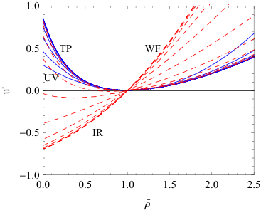
The relative stability of the fixed points can be checked explicitly by considering the full solution (2). In fig. 1 we depict the evolution of the potential, as predicted by this expression, for $\lambda_{\Lambda}=10^{-7}$ and $\nu_{\Lambda}=0.3$. We have set $NC_{3}=1$ through a redefinition of $\tilde{\rho}$ and $u^{\prime}$. We have indicated by UV the initial form of the potential at $k=\Lambda$ and with IR its form for $k\rightarrow 0$. The continuous lines depict the potential at various values of $t$, with step equal to $-1$, during its initial approach to the tricritical fixed point (TP). The dashed lines depict its subsequent evolution towards the Wilson-Fisher fixed point (WF).

We shall not analyse in detail the tricritical line, as this has been done elsewhere [16, 17, 18, 24]. We note that it connects the Gaussian fixed point, for $\nu_{\Lambda}=0$, with a point approached for a value of $\nu_{\Lambda}$ for which the solution of eq. (12) diverges at the origin. This endpoint of the tricritical line is the BMB fixed point [16]. The corresponding value of $\nu_{\Lambda}$ can be derived by using the expansion (7) of the hypergeometric function near the origin, where the fixed-point potential diverges. It is given by $\nu_{\Lambda}=2/(\pi\kappa_{*})$. Taking into account our definition of $\rho$, it can be checked that this value is consistent with the result of refs. [16, 17, 18]. The theory also displays first-order phase transitions if the potential develops two minima. It was shown in ref. [23] that, for a bare potential of the form (9), the surface $\kappa_{\Lambda}=\kappa_{*}+\lambda_{\Lambda}/\nu_{\Lambda}$ corresponds to first-order phase transtions. This surface intersects the surface $\kappa_{\Lambda}=\kappa_{*}$ of second-order phase transitions on the tricritical line $\lambda_{\Lambda}=0$.

We next turn to the search for new infrared fixed points with more than one relevant directions. The presence of the Gaussian fixed point, with $u^{\prime}=0$, is obvious from eq. (1). For any nontrivial fixed point, the rhs of eq. (2) must become independent of $t$ in the limit $t\rightarrow-\infty$. For $d>2$ the hypergeometric function can be approximated through the asymptotic expansion (3) in this limit. An expression independent of $t$ requires an appropriate choice of the function $G$, determined through the initial condition. More precisely, we must have $G(z)-\kappa_{*}\sim z^{\frac{d-2}{2}}$ for $z\rightarrow 0$. This can be achieved through an initial condition of the form

where the parametrization of the multiplicative constant has been introduced for later convenience. We obtain

The tuning $\kappa_{\Lambda}=\kappa_{*}$ results in a fixed-point potential given by the solution of

where we have taken the limit $t\rightarrow-\infty$ with finite $u^{\prime}_{*}$. The fixed-point potential has $u^{\prime}_{*}=0$ at $\tilde{\rho}=\kappa_{*}$, similarly to the bare potential $u_{\Lambda}$.

It is apparent from eqs. (13), (15) that a nonsingular real potential for all values of $\tilde{\rho}\geq 0$ can be obtained only if $d/(d-2)$ takes positive integer values $n$, i.e. at dimensions $d=2n/(n-1)$. If we require $2<d<4$, we have $n\geq 3$. Approaching a fixed point requires, apart from the tuning of $\kappa_{\Lambda}$, the absence of all terms $(\tilde{\rho}-\kappa_{\Lambda})^{m}$ with $1<m<n$ in the bare potential. (The absence of the term with $m=1$ is equivalent to the tuning of $\kappa_{\Lambda}$.) This means that the fixed point at a given dimension $d=2n/(n-1)$ has $n-1$ relevant directions and can be characterized as a multicritical point. For $\tilde{\rho}<\kappa_{*}$ the form of the fixed-point potential depends on $n$. For $n$ odd we have $u^{\prime}_{*}(\tilde{\rho})>0$ for $\tilde{\rho}<\kappa_{*}$, while for $n$ even we have $u^{\prime}_{*}(\tilde{\rho})<0$. In the second case, the potential at the origin is constrained by the pole in the hypergeometric function to satisfy $u^{\prime}_{*}(0)>-1$.

For $d\not=2n/(n-1)$, the initial condition (13) and the solution (15) develop certain pathologies. For $\tilde{\rho}>\kappa_{*}$, the potential is real. For $\tilde{\rho}\gg\kappa_{*}$ we have $u^{\prime}_{*}\gg 1$, so that the hypergeometric function in eq. (15) has the expansion (7). As we discussed above, we obtain the asymptotic form of the potential $u_{*}(\tilde{\rho})\sim\tilde{\rho}^{d/(d-2)}$ and a critical exponent $\delta=(d+2)/(d-2)$. However, divergencies in the higher derivatives of both the bare and fixed-point potentials appear as one approaches the point $\tilde{\rho}=\kappa_{*}$, at which $u^{\prime}_{\Lambda}=u^{\prime}_{*}=0$. The situation is more problematic for $\tilde{\rho}<\kappa_{*}$, where eqs. (13), (15) indicate that the potential must become complex. This leads to the conclusion that a continuous range of real fixed-point solutions as a function of $d$ does not exist in the large-$N$ limit.

It must be pointed out that a real solution can be constructed through an initial condition of the form

where the positive sign is used for $\tilde{\rho}>\kappa_{*}$, while the choice is ambiguous for $\tilde{\rho}<\kappa_{*}$. Both signs lead to real potentials, but for both choices the potentials are nonanalytic at $\tilde{\rho}=\kappa_{*}$. It cannot be excluded that the nonanalyticity has a physical origin. On the other hand, it is not possible to have a continuous dependence of the fixed-point potentials on $d$. The real and continuous solutions at $d=2n/(n-1)$ result from initial conditions given by (16) with one of the two signs, but switch from one sign to the other as $n$ is increased.

The only way to preserve a notion of analyticity and a continuous dependence on $d$ seems to be to consider a continuation of the potential in the complex plane. Even though we cannot offer a physical interpretation of the potential, such a construction is interesting because it may be linked to the picture presented in ref. [1]. There, it is found that fixed-point solutions that exist for a continuous range of increasing values of $N$ collide with each other at some critical value $N_{c}(d)$ and disappear, consistently with what has been seen through the $\epsilon$-expansion [26]. The collision of two-fixed points is expected to cause them to move into the complex plane [27]. In this sense, the presence of complex fixed-point solutions for the full potential at $N\rightarrow\infty$ would be consistent with the findings of ref. [1].

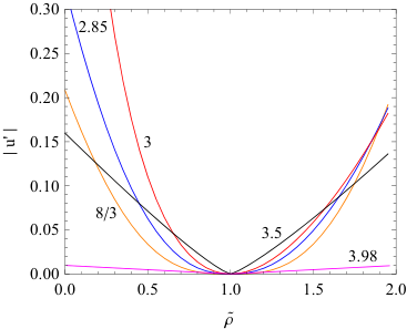
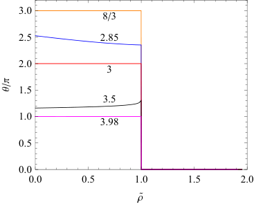
In fig. 2 we present complex solutions of the fixed-point equation (15) for $\nu_{\Lambda}=0.3$. We have set $NC_{d}=1$ through a redefinition of $\tilde{\rho}$ and $u^{\prime}$. The left plot depicts the absolute value and the right plot the argument of the complex potential at the multicritical point. For $\tilde{\rho}>\kappa_{*}=1$ the solution is real and the argument vanishes. For $\tilde{\rho}<1$ the solution is real and continuous only at $d=3$ and $8/3$, and in general at $d=2n/(n-1)$, as discussed earlier. For any other value of $d$, the bare and fixed-point potentials have branch cuts along the negative real axis. In fig. 2 we depict the argument of the potential as the negative real axis is approached from above. The argument has the opposite sign when the negative real axis is approached from below. The potential is discontinuous as the negative real axis is crossed, apart from at $d=2n/(n-1)$. On the other hand, there is a continuity in the dependence of the potential on $d$. In particular, for $\tilde{\rho}<\kappa_{\Lambda}$, the potential switches automatically from solutions with $u^{\prime}>0$ to ones with $u^{\prime}<0$ and back, as $n$ is increased.

Our analysis aimed at examining the presence of nonperturbative fixed-point solutions of the $O(N)$-symmetric scalar theory in dimensions $2<d<4$ for $N\rightarrow\infty$. The motivation arose through the findings of ref. [1], which indicate the presence of previously unknown fixed-point solutions for finite $N$. Some of the new solutions collide with each other at some critical value $N_{c}(d)$ and disappear. One expects the presence of complex solutions beyond this critical value [27]. However, some novel real solutions are expected to persist in the limit $N\rightarrow\infty$ [28]. Our aim was to identify them through an analytical treatment of the RG equation. In this respect, a crucial point is our assumption about what constitutes the leading contribution for large $N$. For vanishing anomalous dimension, and under the assumption that higher-derivative terms in the action can be neglected, the exact Wetterich equation is reduced to a partial differential equation for the potential [11]. The renormalization of the potential is induced by a term proportional to $N$, arising from the contributions of the Goldstone modes, and a term arising from the contribution of the unique radial mode. Our large-$N$ approximation consists in neglecting the second term.

We presented the exact solution (2) of the large-$N$ equation (1) for the evolution of the potential towards the infrared, starting from an initial condition at an ultraviolet energy scale. The presence of critical points in dimensions $2<d<4$, the necessary fine tunings of the initial condition in order to approach them during the evolution, as well as their relative stability, can be deduced from eq. (2) by specifying the function $G(z)$. Our analysis of the previous two sections reproduced the known critical and multicritical points, including the Wilson-Fisher fixed point and the BMB fixed point. However, it did not reveal any new analytic solutions. Even though we used a sharp cutoff for our analysis, we expect similar results for other cutoff functions. For example, the three-dimensional fixed-point structure that we identified is the same as the one found in ref. [24] with a different cutoff.

By continuing the potential in the complex plane, we obtained a class of solutions with a branch-cut discontinuity along the negative real axis and a continuous dependence on $d$. These solutions become real at specific values of $d$, thus reproducing the known multicritical points. The presence of complex fixed points is consistent with the finding of ref. [1] that fixed-point solutions that exist for finite $N$ collide with each other at some critical value $N_{c}(d)$ and disappear. On the other, it is expected that some of the real solutions presented in ref. [1] survive for $N\rightarrow\infty$ [28]. No such solutions were found through our analysis. The only new real solutions we found display discontinuities or singularities in the higher derivatives of the potential at its minimum. They can be obtained from an initial condition given by eq. (16), for both signs, as discussed in the previous section. A natural question is whether some of the numerical solutions presented in ref. [1] display similar discontinuities or singularities, so that they can be identified with our solutions. Another possibility is that our assumption that the radial mode gives a contribution subleading in $1/N$ is violated by the novel solutions [1, 28].

References

- [1] S. Yabunaka and B. Delamotte, Phys. Rev. Lett. 119 (2017) no.19, 191602 [arXiv:1707.04383 [cond-mat.stat-mech]].
- [2] T. H. Berlin and M. Kac, Phys. Rev. 86 (1952) 821.
- [3] E. Brezin and D. J. Wallace, Phys. Rev. B 7 (1973) no.5, 1967.
- [4] H. E. Stanley, Phys. Rev. 176 (1968) 718.
- [5] S. k. Ma, Rev. Mod. Phys. 45 (1973) 589.
- [6] S. k. Ma, J. Math. Phys. 15 (1974) 1866.
- [7] J. Zinn-Justin, Int. Ser. Monogr. Phys. 113 (2002) 1.
- [8] K. G. Wilson and J. B. Kogut, Phys. Rept. 12 (1974) 75.
- [9] F. J. Wegner and A. Houghton, Phys. Rev. A 8 (1973) 401.
- [10] J. Polchinski, Nucl. Phys. B 231 (1984) 269.
- [11] C. Wetterich, Phys. Lett. B 301 (1993) 90.
- [12] T. S. Chang, D. D. Vvedensky and J. F. Nicoll, Phys. Rept. 217 (1992) 279.
- [13] J. Berges, N. Tetradis and C. Wetterich, Phys. Rept. 363 (2002) 223 [hep-ph/0005122].
- [14] M. D’Attanasio and T. R. Morris, Phys. Lett. B 409 (1997) 363 [hep-th/9704094].
- [15] K. G. Wilson and M. E. Fisher, Phys. Rev. Lett. 28 (1972) 240.
- [16] W. A. Bardeen, M. Moshe and M. Bander, Phys. Rev. Lett. 52 (1984) 1188.
- [17] F. David, D. A. Kessler and H. Neuberger, Phys. Rev. Lett. 53 (1984) 2071.
- [18] F. David, D. A. Kessler and H. Neuberger, Nucl. Phys. B 257 (1985) 695.
- [19] N. Tetradis and C. Wetterich, Nucl. Phys. B 422 (1994) 541 [hep-ph/9308214].
- [20] T. R. Morris, Phys. Lett. B 329 (1994) 241 [hep-ph/9403340].
- [21] L. Canet, B. Delamotte, D. Mouhanna and J. Vidal, Phys. Rev. B 68 (2003) 064421 [hep-th/0302227].
- [22] K. I. Aoki, K. i. Morikawa, W. Souma, J. i. Sumi and H. Terao, Prog. Theor. Phys. 95 (1996) 409 [hep-ph/9612458].
- [23] N. Tetradis and D. F. Litim, Nucl. Phys. B 464 (1996) 492 [hep-th/9512073].
- [24] D. F. Litim, E. Marchais and P. Mati, Phys. Rev. D 95 (2017) no.12, 125006 [arXiv:1702.05749 [hep-th]].
- [25] N. Tetradis and C. Wetterich, Nucl. Phys. B 383 (1992) 197.
- [26] H. Osborn and A. Stergiou, arXiv:1707.06165 [hep-th].
- [27] D. B. Kaplan, J. W. Lee, D. T. Son and M. A. Stephanov, Phys. Rev. D 80 (2009) 125005 [arXiv:0905.4752 [hep-th]].
- [28] S. Yabunaka and B. Delamotte, private communication.