Optimal Metastability-Containing Sorting Networks

Johannes Bund Affiliation: Saarland Informatics Campus, MPI for Informatics, Germany, Email: {jbund,clenzen}@mpi-inf.mpg.de Christoph Lenzen Affiliation: Saarland Informatics Campus, MPI for Informatics, Germany, Email: {jbund,clenzen}@mpi-inf.mpg.de Moti Medina Affiliation: Dept. of Electrical & Computer Engineering, Ben-Gurion University of the Negev, Israel, Email: medinamo@bgu.ac.il

Abstract

When setup/hold times of bistable elements are violated, they may become metastable, i.e., enter a transient state that is neither digital 0 nor 1 [13]. In general, metastability cannot be avoided, a problem that manifests whenever taking discrete measurements of analog values. Metastability of the output then reflects uncertainty as to whether a measurement should be rounded up or down to the next possible measurement outcome.

Surprisingly, Lenzen & Medina (ASYNC 2016) showed that metastability can be contained, i.e., measurement values can be correctly sorted without resolving metastability first. However, both their work and the state of the art by Bund et al. (DATE 2017) leave open whether such a solution can be as small and fast as standard sorting networks. We show that this is indeed possible, by providing a circuit that sorts Gray code inputs (possibly containing a metastable bit) and has asymptotically optimal depth and size. Concretely, for $10$ -channel sorting networks and $16$ -bit wide inputs, we improve by $48.46\%$ in delay and by $71.58\%$ in area over Bund et al. Our simulations indicate that straightforward transistor-level optimization is likely to result in performance on par with standard (non-containing) solutions.

1 Introduction

Metastability is one of the basic obstacles when crossing clock domains, potentially resulting in soft errors with critical consequences [8]. As it has been shown that there is no deterministic way of avoiding metastability [13], synchronizers [9] are employed to reduce the error probability to tolerable levels. Besides energy and chip area, this approach costs time: the more time is allocated for metastability resolution, the smaller is the probability of a (possibly devastating) metastability-induced fault.

Recently, a different approach has been proposed, coined metastability-containing (MC) circuits [6]. The idea is to accept (a limited amount of) metastability in the input to a digital circuit and guarantee limited metastability of its output, such that the result is still useful. The authors of [2, 12] apply this approach to a fundamental primitive: sorting. However, the state-of-the-art [2] are circuits that are by a $\Theta(\log B)$ factor larger than non-containing solutions, where $B$ is the bit width of inputs. Accordingly, the authors pose the following question:

“What is the optimum cost of the $\operatorname{2-sort}$ primitive?”

We argue that answering this question is critical, as the performance penalty imposed by current MC sorting primitives is not outweighed by the avoidance of synchronizers.

Our Contribution

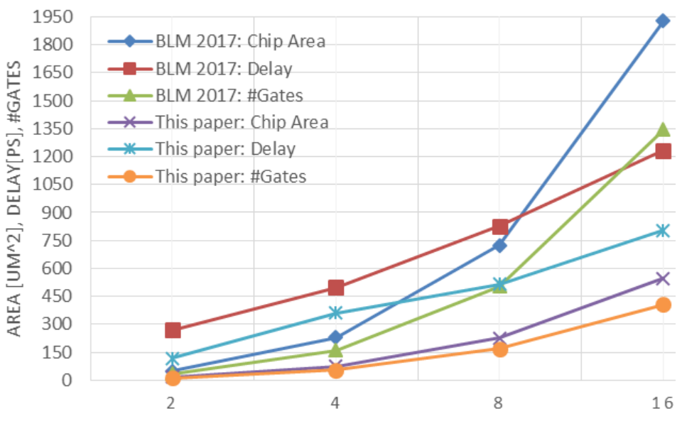
We answer the above question by providing a $B$ -bit MC $\operatorname{2-sort}$ circuit of depth $O(\log B)$ and $O(B)$ gates. Trivially, any such building block with gates of constant fan-in must have this asymptotic depth and gate count, and it improves by a factor of $\Theta(\log B)$ on the gate complexity of [2]. Furthermore, we provide optimized building blocks that significantly improve the leading constants of these complexity bounds. See Figure 1 for our improvements over prior work; specifically, for $16$ -bit inputs, area and delay decrease by up to $71.58\%$ and $48.46\%$ respectively.

Plugging our circuit into (optimal depth or size) sorting networks [3, 4, 10], we obtain efficient combinational metastability-containing sorting circuits, cf. Table 8. In general, plugging our $\operatorname{2-sort}$ circuit into an $n$ -channel sorting network of depth $O(\log n)$ with $O(n\log n)$ $\operatorname{2-sort}$ elements [1], we obtain an asymptotically optimal MC sorting network of depth $O(\log B\log n)$ and $O(Bn\log n)$ gates.

Refer to caption — Figure 1: Area, delay, and gate count of $\operatorname{2-sort}(B)$ for $B\in\{2,4,8,16\}$ ; we compare our solution to [2].

Further Related Work

Ladner and Fischer [11] studied the problem of computing all the prefixes of applications of an associative operator on an input string of length $n$ . They designed and analyze a recursive construction which computes all these prefixes in parallel. The resulting parallel prefix computation (PPC) circuit has depth of $O(\log n)$ and gate count of $O(n)$ (assuming that the implementation of the associative operator has constant size and constant depth). We make use of their construction as part of ours.

2 Model and Problem

In this section, we discuss how to model metastability in a worst-case fashion and formally specify the input/output behavior of our circuits.

We use the following basic notation. For $N\in\mathbb{N}$ , we set $[N]:=\{0,\ldots,N-1\}$ . For a binary $B$ -bit string $g$ , denote by $g_{i}$ its $i$ -th bit, i.e., $g=g_{1}g_{2}\ldots g_{B}$ . We use the shorthand $g_{i,j}:=g_{i}\ldots g_{j}$ . Let $\operatorname{par}(g)$ denote the parity of $g$ , i.e, $\operatorname{par}(g)=\sum_{i=1}^{B}g_{i}\bmod 2$ .

Reflected Binary Gray Code

Due to possible metastability of inputs, we use Gray code. Denote by $\langle\cdot\rangle$ the decoding function of a Gray code string, i.e., for $x\in[N]$ , $\langle\operatorname{rg}_{B}(x)\rangle=x$ . As each $B$ -bit string is a codeword, the code is a bijection and the decoding function also defines the encoding function $\operatorname{rg}_{B}:[N]\to\{0,1\}^{B}$ . We define $B$ -bit binary reflected Gray code recursively, where a $1$ -bit code is given by $\operatorname{rg}_{1}(0)=0$ and $\operatorname{rg}_{1}(1)=1$ . For $B>1$ , we start with the first bit fixed to $0$ and counting with $\operatorname{rg}_{B-1}(\cdot)$ (for the first $2^{B-1}-1$ codewords), then toggle the first bit to $1$ , and finally “count down” $\operatorname{rg}_{B-1}(\cdot)$ while fixing the first bit again, cf. Table 1. Formally, this yields

\operatorname{rg}_{B}(x):=\begin{cases}0\operatorname{rg}_{B-1}(x)&\mbox{if }x\in[2^{B-1}]\\ 1\operatorname{rg}_{B-1}(2^{B}-1-x)&\mbox{if }x\in[2^{B}]\setminus[2^{B-1}].\end{cases}

$\#$	$g_{1},g_{2,4}$	$\#$	$g_{1},g_{2,4}$	$\#$	$g_{1},g_{2,4}$	$\#$	$g_{1},g_{2,4}$
$0$	$0,000$	$4$	$0,110$	$8$	$1,100$	$12$	$1,010$
$1$	$0,001$	$5$	$0,111$	$9$	$1,101$	$13$	$1,011$
$2$	$0,011$	$6$	$0,101$	$10$	$1,111$	$14$	$1,001$
$3$	$0,010$	$7$	$0,100$	$11$	$1,110$	$15$	$1,000$

Table 1: 4-bit binary reflected Gray code

We define the maximum and minimum of two binary reflected Gray code strings, $\operatorname{max^{\operatorname{rg}}}$ and $\operatorname{min^{\operatorname{rg}}}$ respectively, in the usual way, as follows. For two binary reflected Gray code strings $g,h\in\{0,1\}^{B}$ , $\operatorname{max^{\operatorname{rg}}}$ and $\operatorname{min^{\operatorname{rg}}}$ are defined as

\displaystyle\left(\operatorname{max^{\operatorname{rg}}}\{g,h\},\operatorname{min^{\operatorname{rg}}}\{g,h\}\right)

\displaystyle:=\begin{cases}(g,h)&\mbox{if }\langle g\rangle\geq\langle h\rangle\\ (h,g)&\mbox{if }\langle g\rangle\leq\langle h\rangle.\end{cases}

Valid Strings

In [12], the authors represent metastable “bits” by M. The inputs to the sorting circuit may have some metastable bits, which means that the respective signals behave out-of-spec from the perspective of Boolean logic. Such inputs, referred to as valid strings, are introduced with the help of the following operator.

Definition 2.1 (The $*$ operator [12]).

For $B\in\mathbb{N}$ , define the operator $*:\{0,1,\textnormal{{M}}\}^{B}\times\{0,1,\textnormal{{M}}\}^{B}\rightarrow\{0,1,\textnormal{{M}}\}^{B}$ by

\forall i\in\{1,\ldots,B\}:(x*y)_{i}:=\begin{cases}x_{i}&\mbox{if }x_{i}=y_{i}\\ \textnormal{{M}}&\mbox{else.}\end{cases}

Observation 2.2.

The operator $*$ is associative and commutative. Hence, for a set $S=\{x^{(1)},\ldots,x^{(k)}\}$ of $B$ -bit strings, we can use the shorthand

\mathop{\raisebox{-0.7pt}{${{{*}}}$}}S:=\mathop{\raisebox{-0.7pt}{${{{*}}}$}}_{x\in S}x:=x^{(1)}*x^{(2)}*\ldots*x^{(k)}.

We call $\mathop{\raisebox{-0.7pt}{${{{*}}}$}}S$ the superposition of the strings in $S$ .

Valid strings have at most one metastable bit. If this bit resolves to either $0$ or $1$ , the resulting string encodes either $x$ or $x+1$ for some $x$ , cf. Table 2.

Definition 2.3 (Valid Strings [12]).

Let $B\in\mathbb{N}$ and $N=2^{B}$ . Then, the set of valid strings of length $B$ is

\mathcal{S}^{B}_{\operatorname{rg}}:=\operatorname{rg}_{B}([N])\cup\bigcup_{x\in[N-1]}\{\operatorname{rg}_{B}(x)*\operatorname{rg}_{B}(x+1)\}\>,

where for a set $A$ we abbreviate $f(A):=\{f(y)\,|\,y\in A\}$ .

As pointed out in [2], inputs that are valid strings may, e.g., arise from using suitable time-to-digital converters for measuring time differences [7].

$g$	$\langle g\rangle$	$g$	$\langle g\rangle$	$g$	$\langle g\rangle$	$g$	$\langle g\rangle$
$0000$	$0$	$0110$	$4$	$1100$	$8$	$1010$	$12$
$000\textnormal{{M}}$	$-$	$011\textnormal{{M}}$	$-$	$110\textnormal{{M}}$	$-$	$101\textnormal{{M}}$	$-$
$0001$	$1$	$0111$	$5$	$1101$	$9$	$1011$	$13$
$00\textnormal{{M}}1$	$-$	$01\textnormal{{M}}1$	$-$	$11\textnormal{{M}}1$	$-$	$10\textnormal{{M}}1$	$-$
$0011$	$2$	$0101$	$6$	$1111$	$10$	$1001$	$14$
$001\textnormal{{M}}$	$-$	$010\textnormal{{M}}$	$-$	$111\textnormal{{M}}$	$-$	$100\textnormal{{M}}$	$-$
$0010$	$3$	$0100$	$7$	$1110$	$11$	$1000$	$15$
$0\textnormal{{M}}10$	$-$	$\textnormal{{M}}100$	$-$	$1\textnormal{{M}}10$	$-$	$-$	$-$

Table 2:

4

-bit valid inputs

Observation 2.4.

For any $1\leq i\leq j\leq B$ and $g\in\mathcal{S}^{B}_{\operatorname{rg}}$ , $g_{i,j}\in\mathcal{S}^{j-i+1}_{\operatorname{rg}}$ , i.e., $g_{i,j}$ is a valid string, too.

Proof.

Follows immediately from Observation 3.1. ∎

Resolution and Closure

To extend the specification of $\operatorname{max^{\operatorname{rg}}}$ and $\operatorname{min^{\operatorname{rg}}}$ to valid strings, we make use of the metastable closure [6], which in turn makes use of the resolution.

Definition 2.5 (Resolution [6]).

For $x\in\{0,1,\textnormal{{M}}\}^{B}$ ,

\operatorname{res}(x):=\{y\!\in\!\{0,1\}^{B}|\forall i\in\{1,\ldots,B\}\colon x_{i}\neq\textnormal{{M}}\Rightarrow y_{i}=x_{i}\}.

Thus, $\operatorname{res}(x)$ is the set of all strings obtained by replacing all Ms in $x$ by either $0$ or $1$ : M acts as a “wild card.”
We note the following for later use.

Observation 2.6.

For any $x$ , $\mathop{\raisebox{-0.7pt}{${{{*}}}$}}\operatorname{res}(x)=x$ . For any $S$ , $S\subseteq\operatorname{res}(\mathop{\raisebox{-0.7pt}{${{{*}}}$}}S)$ .

The metastable closure of an operator on binary inputs extends it to inputs that may contain metastable bits. This is done by considering all resolutions of the inputs, applying the operator, and taking the superposition of the results.

Definition 2.7 (The M Closure [6]).

Given an operator $f\colon\{0,1\}^{n}\times\{0,1\}^{n}\to\{0,1\}^{n}$ , its metastable closure $f_{\textnormal{{M}}}\colon\{0,1,\textnormal{{M}}\}^{n}\times\{0,1,\textnormal{{M}}\}^{n}\to\{0,1,\textnormal{{M}}\}^{n}$ is defined by

f_{\textnormal{{M}}}(x):=\mathop{\raisebox{-0.7pt}{${{{*}}}$}}f(\operatorname{res}(x)).

Output Specification

We want to construct a circuit that outputs the maximum and minimum of two valid strings, which will enable us to build sorting networks for valid strings. First, however, we need to answer the question what it means to ask for the maximum or minimum of valid strings. To this end, suppose a valid string is $\operatorname{rg}_{B}(x)*\operatorname{rg}_{B}(x+1)$ for some $x\in[N-1]$ , i.e., the string contains a metastable bit that makes it uncertain whether the represented value is $x$ or $x+1$ . This means that the measurement the string represents was taken of a value somewhere between $x$ and $x+1$ . Moreover, if we wait for metastability to resolve, the string will stabilize to either $\operatorname{rg}_{B}(x)$ or $\operatorname{rg}_{B}(x+1)$ . Accordingly, it makes sense to consider $\operatorname{rg}_{B}(x)*\operatorname{rg}_{B}(x+1)$ “in between” $\operatorname{rg}_{B}(x)$ and $\operatorname{rg}_{B}(x+1)$ , resulting in the total order on valid strings given by Table 2.
The above intuition can be formalized by extending $\operatorname{max^{\operatorname{rg}}}$ and $\operatorname{min^{\operatorname{rg}}}$ to valid strings using the metastable closure.

Definition 2.8 ([2, 12]).

For $B\in\mathbb{N}$ , a $\operatorname{2-sort}(B)$ circuit is specified as follows.

•

Input: $g,h\in\mathcal{S}^{B}_{\operatorname{rg}}$ ,
•

Output: $g^{\prime},h^{\prime}\in\mathcal{S}^{B}_{\operatorname{rg}}$ ,
•

Functionality: $g^{\prime}=\operatorname{max^{\operatorname{rg}}_{\textnormal{{M}}}}\{g,h\}$ , $h^{\prime}=\operatorname{min^{\operatorname{rg}}_{\textnormal{{M}}}}\{g,h\}$ .

As shown in [2], this definition indeed coincides with the one given in [12], and for valid strings $g$ and $h$ , $\operatorname{max^{\operatorname{rg}}_{\textnormal{{M}}}}\{g,h\}$ and $\operatorname{min^{\operatorname{rg}}_{\textnormal{{M}}}}\{g,h\}$ are valid strings, too. More specifically, $\operatorname{max^{\operatorname{rg}}_{\textnormal{{M}}}}$ and $\operatorname{min^{\operatorname{rg}}_{\textnormal{{M}}}}$ are the $\max$ and $\min$ operators w.r.t. the total order on valid strings shown in Table 2, e.g.,

•

$\operatorname{max^{\operatorname{rg}}_{\textnormal{{M}}}}\{1001,1000\}=\operatorname{rg}_{4}(15)=1000$ ,
•

$\operatorname{max^{\operatorname{rg}}_{\textnormal{{M}}}}\{0\textnormal{{M}}10,0010\}=\operatorname{rg}_{4}(3)*\operatorname{rg}_{4}(4)=0\textnormal{{M}}10$ ,
•

$\operatorname{max^{\operatorname{rg}}_{\textnormal{{M}}}}\{0\textnormal{{M}}10,0110\}=\operatorname{rg}_{4}(4)=0110$ .

Computational Model

We seek to use standard components and combinational logic only. We use the model of [6], which specifies the behavior of basic gates on metastable inputs via the metastable closure of their behavior on binary inputs. For standard implementations of $\operatorname{AND}$ and $\operatorname{OR}$ gates, this assumption is valid: if M represents an arbitrary, possibly time-dependent voltage between logical $0$ and $1$ , an $\operatorname{AND}$ gate will still output logical $0$ if the respective other input is logical $0$ . Similarly, an $\operatorname{OR}$ gate with one input being logical $1$ suppresses metastability at the other input, cf. Table 3.

As pointed out in [2], any additional reduction of metastability in the output necessitates the use of non-combinational masking components (e.g., masking registers), analog components, and/or synchronizers, all of which are outside of our computational model. Moreover, other than the usage of analog components, these alternatives require to spend additional time, which we avoid in this paper.

	1	M
0	0	0
1	1	M
M	M	M

	0	1	M
0	0	1	M
1	1	1	1
M	M	1	M

a	$\bar{\text{a}}$
0	1
1	0
M	M

Table 3: Logical extensions to metastable inputs of AND (left), OR (center), and an inverter (right).

3 Preliminaries on Stable Inputs

We note the following observation for later use. Informally, it states that removing prefixes and suffixes from the code results in (repetition) of binary reflected Gray codes.

Observation 3.1.

For $B$ -bit binary reflected Gray code, fix $1\leq i<j\leq B$ , and consider the sequence of strings obtained by (i) listing all codewords in ascending order of encoded values, (ii) replacing each codeword $g$ by $g_{i,j}$ , and (iii) deleting all immediate repetitions (i.e., if two consecutive strings are identical, keep only one of them). Then the resulting list repeatedly counts “up” and “down” through the codewords of $(j-i)$ -bit binary reflected Gray code.

Proof.

When removing the first bit of $B$ -bit binary reflected Gray code, the claim follows directly from the definition. By induction, we can confirm that the last bit of $B$ -bit code toggles on every second up-count, and $\langle g\rangle=2\cdot\langle g_{1,B-1}\rangle+\operatorname{XOR}(\operatorname{par}(g_{1,B-1}),g_{B})$ . Thus, the claim holds if we either remove the first or last bit. As the same arguments apply when we have a list counting “up” and “down” repeatedly, we can inductively remove the first $i-1$ bits and the last $B-j$ bits to prove the general claim. ∎

Comparing Stable Gray Code Strings via an FSM

The following basic structural lemma leads to a straightforward way of comparing binary reflected Gray code strings.

Lemma 3.2.

Let $g,h\in\{0,1\}^{B}$ such that $\langle g\rangle>\langle h\rangle$ . Denote by $i\in\{1,\ldots,B\}$ the first index such that $g_{i}\neq h_{i}$ . Then $g_{i}=1$ (i.e., $h_{i}=0$ ) if $\operatorname{par}(g_{1,i-1})=0$ and $g_{i}=0$ (i.e., $h_{i}=1$ ) if $\operatorname{par}(g_{1,i-1})=1$ .

Proof.

We prove the claim by induction on $B$ , where the base case $B=1$ is trivial. Now consider $B$ -bit strings for some $B>1$ and assume that the claim holds for $B-1$ bits. If $i=1$ , again the claim trivially follows from the definition. If $i>1$ , we have that $g_{1}=h_{1}$ . Denote $x=\langle g\rangle$ and $y=\langle h\rangle$ . If $g_{1}=h_{1}=0$ , then $g_{2,B}=\operatorname{rg}_{B-1}(x)$ and $h_{2,B}=\operatorname{rg}_{B-1}(y)$ . Thus, as $x>y$ by assumption, the claim follows from the induction hypothesis. If $g_{1}=h_{1}=1$ , $g_{2,B}=\operatorname{rg}_{B-1}(2^{B}-1-x)$ and $h_{2,B}=\operatorname{rg}_{B-1}(2^{B}-1-y)$ . Note that $g^{\prime}:=h_{2,B}$ and $h^{\prime}:=g_{2,B}$ satisfy that $\langle g^{\prime}\rangle>\langle h^{\prime}\rangle$ and that their first differing bit is $i-1$ . By the induction hypothesis, we have that $h^{\prime}_{i-1}=g_{i}=1$ if $\operatorname{par}(g^{\prime}_{1,i-2})=\operatorname{par}(h^{\prime}_{1,i-2})=\operatorname{par}(g_{2,i-1})=1$ and, accordingly, $g_{i}=0$ if $\operatorname{par}(g_{2,i-1})=0$ . As $g_{1}=1$ , $\operatorname{par}(g_{1,i-1})=1-\operatorname{par}(g_{2,i-1})$ , and the claim follows. ∎

Figure 2: Finite state automaton determining which of two Gray code inputs

g,h\in\{0,1\}^{B}

is larger. In each step, the machine receives

g_{i}h_{i}

as input. State encoding is given in square brackets.

Lemma 3.2 gives rise to a sequential representation of $\operatorname{2-sort}(B)$ as a Finite state machine (FSM), for input strings in $\{0,1\}^{B}$ . Consider the state machine given in Figure 2. Its four states keep track of whether $g_{1,i}=h_{1,i}$ with parity $0$ (state encoding: $00$ ) or $1$ (state encoding: $11$ ), respectively, $\langle g\rangle<\langle h\rangle$ (state encoding: $01$ ), or $\langle g\rangle>\langle h\rangle$ (state encoding: $10$ ). Denoting by $s^{(i)}$ its state after $i$ steps (where $s^{(0)}=00$ is the initial state), Lemma 3.2 shows that the output given in Table 4 is correct: up to the first differing bits $g_{i}\neq h_{i}$ , the (identical) input bits are reproduced both for $\operatorname{max^{\operatorname{rg}}}$ and $\operatorname{min^{\operatorname{rg}}}$ , and in the $i$ -th step the state machine transitions to the correct absorbing state.

$s^{(i-1)}$	$\operatorname{max^{\operatorname{rg}}}\{g,h\}_{i}$	$\operatorname{min^{\operatorname{rg}}}\{g,h\}_{i}$
00	$\max\{g_{i},h_{i}\}$	$\min\{g_{i},h_{i}\}$
10	$g_{i}$	$h_{i}$
11	$\min\{g_{i},h_{i}\}$	$\max\{g_{i},h_{i}\}$
01	$h_{i}$	$g_{i}$

Table 4: Computing

\operatorname{max^{\operatorname{rg}}}\{g,h\}_{i}

and

\operatorname{min^{\operatorname{rg}}}\{g,h\}_{i}

The $\diamond$ Operator and Optimal Sorting of Stable Inputs

We can express the transition function of the state machine as an operator $\diamond$ taking the current state and input $g_{i}h_{i}$ as argument and returning the new state. Then $s^{(i)}=s^{(i-1)}\diamond g_{i}h_{i}$ , where $\diamond$ is given in Table 5.

$\diamond$	00	01	11	10
00	00	01	11	10
01	01	01	01	01
11	11	10	00	01
10	10	10	10	10

$\mathrm{out}$	01	11	10
00	10	11	10
01	10	11	01
11	01	11	01
10	01	11	10

Table 5: The

\diamond

operator and the

\mathrm{out}

operator. The first operand is the current state, the second the next input bits.

Observation 3.3.

$\diamond$ is associative, that is,

\forall a,b,c\in\{0,1\}^{2}\colon(a\diamond b)\diamond c=a\diamond(b\diamond c).

We thus have that

s^{(i)}=\bigdiamond_{j=1}^{i}g_{j}h_{j}:=g_{1}h_{1}\diamond g_{2}h_{2}\diamond\ldots\diamond g_{i}h_{i},

regardless of the order in which the $\diamond$ operations are applied.

Proof.

First, we observe the following for every $y\in\{0,1\}^{2}$ : (1) $00\diamond y=y$ , (2) $01\diamond y=01$ , (3) $11\diamond y=\bar{y}$ , and (4) $10\diamond y=10$ . We prove that $\diamond$ is associative by considering these four cases for the first operand $x$ . If $x\in\{01,10\}$ , associativity follows from the “absorbing” property of cases $(2)$ and $(4)$ . If $x=00$ , then $(00\diamond y)\diamond z=y\diamond z=00\diamond(y\diamond z)$ . We are left with the case that $x=11$ . Then the LHS equals $\bar{y}\diamond z$ , while the RHS equals $\overline{y\diamond z}$ . Checking Table 5, one can directly verify that $\bar{y}\diamond z=\overline{y\diamond z}$ in all cases. ∎

An immediate consequence is that we can apply the results by [11] on parallel prefix computation to derive an $O(B)$ -gate circuit of depth $O(\log B)$ computing all $s_{i}$ , $i\in[B]$ , in parallel. Our goal in the following sections is to extend this well-known approach to potentially metastable inputs.

4 Dealing with Metastable Inputs

Our strategy is the same as outlined in Section 3 for stable inputs, where we replace all involved operators by their metastable closure: (i) compute $s^{(i)}$ for $i\in[B]$ , (ii) determine $\operatorname{max^{\operatorname{rg}}}\{g,h\}_{i}$ and $\operatorname{min^{\operatorname{rg}}}\{g,h\}_{i}$ according to Table 4 for $i\in\{1,\ldots,B\}$ , and (iii) exploit associativity of the operator computing the $s^{(i)}$ to determine all of them concurrently with $O(\log B)$ depth and $O(B)$ gates (using [11]). To make this work for inputs that are valid strings, we simply replace all involved operators by their respective metastable closure. Thus, we only need to implement $\diamond_{\textnormal{{M}}}$ and the closure of the operator given in Table 4 (both of constant size) and immediately obtain an efficient circuit using the PPC framework [11].

Unfortunately, it is not obvious that this approach yields correct outputs. There are three hurdles to take:

(i)

Show that first computing $s^{(i)}_{\textnormal{{M}}}$ and then the output from this and the input yields correct output for all valid strings.
(ii)

Show that $\diamond_{\textnormal{{M}}}$ behaves like an associative operator on the given inputs (so we can use the PPC framework).
(iii)

Show that repeated application of $\diamond_{\textnormal{{M}}}$ actually computes $s^{(i)}_{\textnormal{{M}}}$ .

Killing two birds with one stone, we first show the second and third point in a single inductive argument. We then proceed to prove the first point.

4.1 Determining $s^{(i)}_{\textnormal{{M}}}$

Note that for any $x$ and $y$ , we have that $\operatorname{res}(xy)=\operatorname{res}(x)\times\operatorname{res}(y)$ . Hence, for valid strings $g,h\in\mathcal{S}^{B}_{\operatorname{rg}}$ and $i\in\{1,\ldots,B\}$ , we have that

s^{(i)}_{\textnormal{{M}}}=\mathop{\raisebox{-0.7pt}{${{{*}}}$}}\bigdiamond_{j=1}^{i}\operatorname{res}(g_{j}h_{j}),

and for convenience set $s^{(0)}_{\textnormal{{M}}}:=s^{(0)}=00$ . Moreover, recalling Definition 2.7,

\displaystyle x\diamond_{\textnormal{{M}}}y=\mathop{\raisebox{-0.7pt}{${{{*}}}$}}_{x^{\prime}y^{\prime}\in\operatorname{res}(xy)}\{x^{\prime}\diamond y^{\prime}\}=\mathop{\raisebox{-0.7pt}{${{{*}}}$}}(\operatorname{res}(x)\diamond\operatorname{res}(y)).

(1)

The following theorem shows that the desired decomposition is feasible.

Theorem 4.1.

Let $g,h\in\mathcal{S}^{B}_{\operatorname{rg}}$ and $1\leq i\leq j\leq B$ . Then

\displaystyle g_{i}h_{i}\diamond_{\textnormal{{M}}}g_{i+1}h_{i+1}\diamond_{\textnormal{{M}}}\ldots\diamond_{\textnormal{{M}}}g_{j}h_{j}

\displaystyle=\mathop{\raisebox{-0.7pt}{${{{*}}}$}}\bigdiamond_{k=i}^{j}\operatorname{res}(g_{k}h_{k}),

(2)

regardless of the order in which the $\diamond_{\textnormal{{M}}}$ operators are applied.

Proof.

We start with a key observation.

Observation 4.2.

Let $g,h\in\mathcal{S}^{B}_{\operatorname{rg}}$ and $1\leq i\leq j\leq B$ . If

\displaystyle\mathop{\raisebox{-0.7pt}{${{{*}}}$}}\bigdiamond_{k=i}^{j}\operatorname{res}(g_{k}h_{k})=\textnormal{{M}}\textnormal{{M}},

there is an index $m$ such that $g_{m}=h_{m}=\textnormal{{M}}$ and $g_{i,m}=h_{i,m}$ . Conversely, if there is no such index, then $x\neq\textnormal{{M}}\textnormal{{M}}$ .

Proof.

Abbreviate $x=\mathop{\raisebox{-0.7pt}{${{{*}}}$}}\bigdiamond_{k=i}^{j}\operatorname{res}(g_{k}h_{k})$ . By Observation 2.4, w.l.o.g. $i=1$ and $j=B$ . Recall that, for any resolutions $g^{\prime}\in\operatorname{res}(g)$ and $h^{\prime}\in\operatorname{res}(h)$ , $\bigdiamond_{k=1}^{B}g_{k}^{\prime}h_{k}^{\prime}$ indicates whether $\langle g^{\prime}\rangle>\langle h^{\prime}\rangle$ ( $10$ ), $\langle g^{\prime}\rangle<\langle h^{\prime}\rangle$ ( $01$ ), $g^{\prime}=h^{\prime}$ with $\operatorname{par}(g^{\prime})=0$ ( $00$ ), or $g^{\prime}=h^{\prime}$ with $\operatorname{par}(g^{\prime})=1$ ( $11$ ). For $x=\textnormal{{M}}\textnormal{{M}}$ , we must have that there are two pairs of resolutions $g^{\prime}$ , $h^{\prime}$ that result in (i) outputs $00$ and $11$ , respectively, or (ii) in outputs $01$ and $10$ , respectively. It is straightforward to see that this entails the claim (cf. Table 2). ∎

We now prove the claim of the theorem by induction on $j-i+1$ , i.e., the length of the strings we feed to the operators. For $j=i$ , we trivially have $g_{i}h_{i}=\mathop{\raisebox{-0.7pt}{${{{*}}}$}}\operatorname{res}(g_{i}h_{i})$ .

For the induction step, suppose $j>i$ and the claim holds for all shorter valid strings. As, by Observation 2.4, $g_{i,j}$ and $h_{i,j}$ are valid strings, w.l.o.g. $i=1$ and $j=B$ . Consider the $\diamond_{\textnormal{{M}}}$ operator (at the position between index $\ell$ and $\ell+1$ ) on the left hand side that is evaluated last; we indicate this by parenthesis and compute

		$\displaystyle(g_{1}h_{1}\diamond_{\textnormal{{M}}}\ldots\diamond_{\textnormal{{M}}}g_{\ell}h_{\ell})\diamond_{\textnormal{{M}}}(g_{\ell+1}h_{\ell+1}\diamond_{\textnormal{{M}}}\ldots\diamond_{\textnormal{{M}}}g_{B}h_{B})$
	$\displaystyle=\,$	$\displaystyle\left(\mathop{\raisebox{-0.7pt}{${{{}}}$}}\bigdiamond_{k=1}^{\ell}\operatorname{res}(g_{k}h_{k})\right)\diamond_{\textnormal{{M}}}\left(\mathop{\raisebox{-0.7pt}{${{{}}}$}}\bigdiamond_{k=\ell+1}^{B}\operatorname{res}(g_{k}h_{k})\right)$
	$\displaystyle\stackrel{{\scriptstyle\eqref{eq:diamondM}}}{{=}}$	$\displaystyle\mathop{\raisebox{-0.7pt}{${{{}}}$}}\left(\operatorname{res}\left(\mathop{\raisebox{-0.7pt}{${{{}}}$}}\bigdiamond_{k=1}^{\ell}\operatorname{res}(g_{k}h_{k})\right)\diamond\operatorname{res}\left(\mathop{\raisebox{-0.7pt}{${{{*}}}$}}\bigdiamond_{k=\ell+1}^{B}\operatorname{res}(g_{k}h_{k})\right)\right)$
	$\displaystyle=\,$	$\displaystyle\mathop{\raisebox{-0.7pt}{${{{*}}}$}}\left(\operatorname{res}(a)\diamond\operatorname{res}(b)\right)=:x,$

where $a=\mathop{\raisebox{-0.7pt}{${{{*}}}$}}\bigdiamond_{k=1}^{\ell}\operatorname{res}(g_{k}h_{k})$ and $b=\mathop{\raisebox{-0.7pt}{${{{*}}}$}}\bigdiamond_{k=\ell+1}^{B}\operatorname{res}(g_{k}h_{k})$ .

By the induction hypothesis, $a$ and $b$ do not depend on the order of evaluation of the $\diamond_{\textnormal{{M}}}$ operators. Thus, it suffices to show that $x$ equals the right hand side of Equality (2).

We distinguish three cases. The first is that the right hand side of (2) evaluates to MM. Then, by Observation 4.2, there is a (unique) index $m$ so that $g_{m}=h_{m}=\textnormal{{M}}$ and $g_{1,m}=h_{1,m}$ . If $m\leq\ell$ , we have (again by Observation 4.2) that $a=\textnormal{{M}}\textnormal{{M}}$ , i.e., $\operatorname{res}(a)=\{0,1\}^{2}$ . Checking Table 5, we see that each column contains both $01$ and $10$ . Hence, regardless of $b$ , $x=\textnormal{{M}}\textnormal{{M}}$ . On the other hand, if $m>\ell$ , then $a\in\{00,11\}$ and $b=\textnormal{{M}}\textnormal{{M}}$ . Checking the $00$ and $11$ rows of Table 5, both of them contain $01$ and $10$ , implying that $x=\textnormal{{M}}\textnormal{{M}}$ .

The second case is that the right hand side of (2) does not evaluate to MM, but $b=\textnormal{{M}}\textnormal{{M}}$ . Then, by Observation 4.2 and the fact that $g$ and $h$ are valid strings, $g_{1,\ell},h_{1,\ell}\in\{0,1\}^{\ell}$ and $g_{1,\ell}\neq h_{1,\ell}$ . W.l.o.g., assume $\langle g_{1,\ell}\rangle>\langle h_{1,\ell}\rangle$ . Then $a=g_{1,\ell}\diamond h_{1,\ell}=10$ and the state machine given in Figure 2 determines output $10$ for inputs $g^{\prime}\in\operatorname{res}(g)$ and $h^{\prime}\in\operatorname{res}(h)$ . As the FSM outputs $\bigdiamond_{k=1}^{B}g_{k}^{\prime}h_{k}^{\prime}$ , we conclude that

	$\displaystyle\mathop{\raisebox{-0.7pt}{${{{*}}}$}}\bigdiamond_{k=1}^{B}\operatorname{res}(g_{k}h_{k})$	$\displaystyle=\mathop{\raisebox{-0.7pt}{${{{*}}}$}}_{g^{\prime}h^{\prime}\in\operatorname{res}(gh)}\left\{\bigdiamond_{k=1}^{B}g^{\prime}_{k}h^{\prime}_{k}\right\}$
		$\displaystyle=\mathop{\raisebox{-0.7pt}{${{{*}}}$}}_{g^{\prime}h^{\prime}\in\operatorname{res}(gh)}\{01\}=01$

as well. Checking the $10$ row of Table 5, we see that $x=10$ , too, regardless of $b$ .

The third case is that the right hand side of (2) does not evaluate to MM and $b\neq\textnormal{{M}}\textnormal{{M}}$ . By Observation 4.2, also $a\neq\textnormal{{M}}\textnormal{{M}}$ . Accordingly, $|\operatorname{res}(a)|,|\operatorname{res}(b)|\in\{1,2\}$ . We claim that this implies that

\displaystyle\operatorname{res}(a)

\displaystyle=\bigdiamond_{k=1}^{\ell}\operatorname{res}(g_{k}h_{k}),\quad\operatorname{res}(b)=\bigdiamond_{k=\ell+1}^{B}\operatorname{res}(g_{k}h_{k}).

This can be seen by noting that, for any set $S\subseteq\{0,1\}^{2}$ , (i) $\operatorname{res}(\mathop{\raisebox{-0.7pt}{${{{*}}}$}}S)\supseteq S$ and (ii) $|\operatorname{res}(\mathop{\raisebox{-0.7pt}{${{{*}}}$}}S)|=2$ necessitates that $|S|\geq 2$ , as otherwise $\mathop{\raisebox{-0.7pt}{${{{*}}}$}}S\in\{0,1\}^{2}$ and thus $|\operatorname{res}(\mathop{\raisebox{-0.7pt}{${{{*}}}$}}S)|=1$ . We conclude that

	$\displaystyle x$	$\displaystyle=\mathop{\raisebox{-0.7pt}{${{{*}}}$}}\left(\operatorname{res}(a)\diamond\operatorname{res}(b)\right)$
		$\displaystyle=\mathop{\raisebox{-0.7pt}{${{{*}}}$}}\left(\left(\bigdiamond_{k=1}^{\ell}\operatorname{res}(g_{k}h_{k})\right)\diamond\left(\bigdiamond_{k=\ell+1}^{B}\operatorname{res}(g_{k}h_{k})\right)\right)$
		$\displaystyle=\mathop{\raisebox{-0.7pt}{${{{*}}}$}}_{\begin{subarray}{c}g^{\prime}\in\operatorname{res}(g)\\ h^{\prime}\in\operatorname{res}(h)\end{subarray}}\left(\left(\bigdiamond_{k=1}^{\ell}g_{k}^{\prime}h_{k}^{\prime}\right)\diamond\left(\bigdiamond_{k=\ell+1}^{B}g_{k}^{\prime}h_{k}^{\prime}\right)\right)$
		$\displaystyle=\mathop{\raisebox{-0.7pt}{${{{}}}$}}_{\begin{subarray}{c}g^{\prime}\in\operatorname{res}(g)\\ h^{\prime}\in\operatorname{res}(h)\end{subarray}}\left(\bigdiamond_{k=1}^{B}g_{k}^{\prime}h_{k}^{\prime}\right)=\mathop{\raisebox{-0.7pt}{${{{}}}$}}\left(\bigdiamond_{k=1}^{B}\operatorname{res}(g_{k}h_{k})\right),$

as desired. ∎

We remark that we did not prove that $\diamond_{\textnormal{{M}}}$ is an associative operator, just that it behaves associatively when applied to input sequences given by valid strings. Moreover, in general the closure of an associative operator needs not be associative. A counter-example is given by binary addition modulo $4$ :

\displaystyle(0\textnormal{{M}}+_{\textnormal{{M}}}01)+_{\textnormal{{M}}}01=\textnormal{{M}}\textnormal{{M}}\neq 1\textnormal{{M}}=0\textnormal{{M}}+_{\textnormal{{M}}}(01+_{\textnormal{{M}}}01).

Since $\diamond_{\textnormal{{M}}}$ behaves associatively when applied to input sequences given by valid strings, we can apply the results by [11] on parallel prefix computation to any implementation of $\diamond_{\textnormal{{M}}}$ .

4.2 Obtaining the Outputs from $s^{(i)}_{\textnormal{{M}}}$

Denote by $\mathrm{out}\colon\{0,1\}^{2}\times\{0,1\}^{2}\to\{0,1\}^{2}$ the operator given in Table 4 computing $\operatorname{max^{\operatorname{rg}}}\{g,h\}_{i}\operatorname{min^{\operatorname{rg}}}\{g,h\}_{i}$ out of $s^{(i-1)}$ and $g_{i}h_{i}$ . The following theorem shows that, for valid inputs, it suffices to implement $\mathrm{out}_{\textnormal{{M}}}$ to determine $\operatorname{max^{\operatorname{rg}}_{\textnormal{{M}}}}\{g,h\}_{i}$ and $\operatorname{min^{\operatorname{rg}}_{\textnormal{{M}}}}\{g,h\}_{i}$ from $s^{(i-1)}_{\textnormal{{M}}}$ , $g_{i}$ , and $h_{i}$ .

Theorem 4.3.

Given valid inputs $g,h\in\mathcal{S}^{B}_{\operatorname{rg}}$ and $i\in[B]$ , it holds that

\mathrm{out}_{\textnormal{{M}}}(s^{(i-1)}_{\textnormal{{M}}},g_{i}h_{i})=\operatorname{max^{\operatorname{rg}}_{\textnormal{{M}}}}\{g,h\}_{i}\operatorname{min^{\operatorname{rg}}_{\textnormal{{M}}}}\{g,h\}_{i}.

Proof.

By definition of $s^{(i-1)}_{\textnormal{{M}}}$ , $\mathrm{out}_{\textnormal{{M}}}(s^{(i-1)}_{\textnormal{{M}}},g_{i}h_{i})$ does not depend on bits $i+1,\ldots,B$ . As by Observation 2.4 $g_{1,i},h_{1,i}\in\mathcal{S}^{i}_{\operatorname{rg}}$ , we may thus w.l.o.g. assume that $B=i$ . For symmetry reasons, it suffices to show the claim for the first output bit $\mathrm{out}_{\textnormal{{M}}}(s^{(B-1)}_{\textnormal{{M}}},g_{B}h_{B})_{1}$ only; the other cases are analogous.

Recall that for $g,h\in\{0,1\}^{B}$ , $s^{(B-1)}_{\textnormal{{M}}}=s^{(B-1)}$ is the state of the state machine given in Figure 2 before processing the last bit. Hence,

		$\displaystyle\,\mathrm{out}_{\textnormal{{M}}}(s^{(B-1)}_{\textnormal{{M}}},g_{B}h_{B})_{1}=\mathrm{out}(s^{(B-1)},g_{B}h_{B})_{1}$
	$\displaystyle=$	$\displaystyle\,\operatorname{max^{\operatorname{rg}}}\{g,h\}_{B}=\operatorname{max^{\operatorname{rg}}_{\textnormal{{M}}}}\{g,h\}_{B}.$

Our task is to prove this equality also for the case where $g$ or $h$ contain a metastable bit.

Let $j$ be the minimum index such that $g_{j}=\textnormal{{M}}$ or $h_{j}=\textnormal{{M}}$ . Again, for symmetry reasons, we may assume w.l.o.g. that $g_{j}=\textnormal{{M}}$ ; the case $h_{j}=\textnormal{{M}}$ is symmetric. If $\langle g_{1,j-1}\rangle\neq\langle h_{1,j-1}\rangle$ , suppose w.l.o.g. (the other case is symmetric) that $\langle g_{1,j-1}\rangle>\langle h_{1,j-1}\rangle$ . Then $s^{(j-1)}=10$ and the state machine is in absorbing state. Thus, regardless of further inputs, we get that $s^{(B-1)}_{\textnormal{{M}}}=s^{(B-1)}=10$ and

\mathrm{out}_{\textnormal{{M}}}(s^{(B-1)}_{\textnormal{{M}}},g_{B}h_{B})_{1}=\mathrm{out}_{\textnormal{{M}}}(10,g_{B}h_{B})_{1}=g_{B}.

Hence, suppose that $g_{1,j-1}=h_{1,j-1}$ ; we consider the case that $\operatorname{par}(g_{1,j-1})=0$ first, i.e., $s^{(j-1)}=00=s^{(0)}$ . By Observation 2.4, $g_{j,B},h_{j,B}\in\mathcal{S}^{B-j+1}_{\operatorname{rg}}$ and thus w.l.o.g. $j=1$ . If $B=1$ ,

\displaystyle\mathrm{out}_{\textnormal{{M}}}(s^{(B-1)}_{\textnormal{{M}}},g_{B}h_{B})_{1}

\displaystyle=\mathrm{out}_{\textnormal{{M}}}(00,\textnormal{{M}}h_{B})_{1}=\begin{cases}1&\mbox{if }h_{1}=1\\ \textnormal{{M}}&\mbox{otherwise,}\end{cases}

which equals $\operatorname{max^{\operatorname{rg}}_{\textnormal{{M}}}}\{g,h\}_{B}$ (we simply have a $1$ -bit code). If $B>1$ , the above implies that $g_{2,\ldots,B}=10\ldots 0$ , as the front bit of the code changes only once, with $10\ldots 0$ being the other bits (cf. Table 2). We distinguish several cases.

h_{1}=\textnormal{{M}}

Then also $h_{2,\ldots,B}=10\ldots 0$ . Therefore $g_{B}=h_{B}$ , $\mathrm{out}(s,g_{B}h_{B})_{1}=g_{B}=h_{B}$ for any $s\in\{0,1\}^{2}$ , and

\mathrm{out}_{\textnormal{{M}}}(s^{(B-1)}_{\textnormal{{M}}},g_{B}h_{B})_{1}=g_{B}=h_{B}=\operatorname{max^{\operatorname{rg}}_{\textnormal{{M}}}}\{g,h\}_{B}.

h_{1}=1

and

B=2

Note that $g$ is smaller than $h$ w.r.t. the total order on valid strings (cf. Table 2), i.e., we need to output $h_{B}=\operatorname{max^{\operatorname{rg}}_{\textnormal{{M}}}}\{g,h\}_{B}$ . Consider the two resolutions of $g$ , i.e., $01$ and $11$ . If the first bit of $g$ is resolved to $0$ , we end up with $s^{(B-1)}=s^{(1)}=01$ . If it is resolved to $1$ , then $s^{(1)}=11$ . Thus,

	$\displaystyle\mathrm{out}_{\textnormal{{M}}}(s^{(B-1)}_{\textnormal{{M}}},g_{B}h_{B})_{1}$	$\displaystyle=\mathrm{out}_{\textnormal{{M}}}(01,1h_{B})_{1}*\mathrm{out}_{\textnormal{{M}}}(11,1h_{B})_{1}$
		$\displaystyle=\mathop{\raisebox{-0.7pt}{${{{*}}}$}}\bigcup_{h^{\prime}\in\operatorname{res}(h)}\{h_{B}^{\prime},\min\{1,h_{B}^{\prime}\}\}$
		$\displaystyle=\mathop{\raisebox{-0.7pt}{${{{*}}}$}}_{h^{\prime}\in\operatorname{res}(h)}\{h_{B}^{\prime}\}=h_{B}.$

h_{1}=1

and

B>2

Again, $h_{B}=\operatorname{max^{\operatorname{rg}}_{\textnormal{{M}}}}\{g,h\}_{B}$ . Consider the two resolutions of $g$ , i.e., $010\ldots 0$ and $110\ldots 0$ . If the first bit of $g$ is resolved to $0$ , we end up with $s^{(B-1)}=s^{(1)}=01$ , as $01$ is an absorbing state. If it is resolved to $1$ , then $s^{(1)}=11$ . As $g_{2,\ldots,B}=10\ldots 0$ , for any $h^{\prime}\in\operatorname{res}(h)$ , the state machine will end up in either state $00$ (if $h^{\prime}_{2,\ldots,B}=10\ldots 0$ ) or state $01$ . Overall, we get that (i) $s^{(B-1)}_{\textnormal{{M}}}=01$ , (ii) $s^{(B-1)}_{\textnormal{{M}}}=00*01=0\textnormal{{M}}$ and $h_{2,\ldots,B}=1\ldots 0$ , or (iii) $s^{(B-1)}_{\textnormal{{M}}}=0\textnormal{{M}}$ and $h_{2,\ldots,B}=1\ldots 0\textnormal{{M}}$ (cf. Table 2). If (i) applies, $\mathrm{out}_{\textnormal{{M}}}(s^{(B-1)}_{\textnormal{{M}}},g_{B}h_{B})_{1}=h_{B}$ . If (ii) applies, $\mathrm{out}_{\textnormal{{M}}}(s^{(B-1)}_{\textnormal{{M}}},g_{B}h_{B})_{1}=g_{B}=h_{B}$ . If (iii) applies, then

	$\displaystyle\mathrm{out}_{\textnormal{{M}}}(s^{(B-1)}_{\textnormal{{M}}},g_{B}h_{B})_{1}$	$\displaystyle=\mathrm{out}_{\textnormal{{M}}}(00,0\textnormal{{M}})_{1}*\mathrm{out}_{\textnormal{{M}}}(01,0\textnormal{{M}})_{1}$
		$\displaystyle=010*1=\textnormal{{M}}=h_{B}.$

$h_{1}=0$ :

This case is symmetric to the previous two: depending on how $g$ is resolved, we end up with $s^{(1)}=10$ or $s^{(1)}=00$ , and need to output $g_{B}$ . Reasoning analogously, we see that indeed $\mathrm{out}_{\textnormal{{M}}}(s^{(B-1)}_{\textnormal{{M}}},g_{B}h_{B})_{1}=g_{B}$ .

It remains to consider $\operatorname{par}(g_{1,\ldots,j-1})=1$ . Then $s^{(j-1)}=11$ . Noting that this reverses the roles of $\max$ and $\min$ , we reason analogously to the case of $\operatorname{par}(g_{1,\ldots,j-1})=0$ . ∎

5 The Complete Circuit

Section 4 breaks the task down to using the PPC framework to compute $s^{(i)}_{\textnormal{{M}}}$ , $i\in[B]$ , using $\diamond_{\textnormal{{M}}}$ and then $\mathrm{out}_{\textnormal{{M}}}$ to determine the outputs. Thus, we need to provide implementations of $\diamond_{\textnormal{{M}}}$ and $\mathrm{out}_{\textnormal{{M}}}$ , and apply the template from [11].

5.1 Implementations of Operators

We provide optimized implementations based on fan-in $2$ $\operatorname{AND}$ and $\operatorname{OR}$ gates and inverters here, cf. Section 2. Depending on target architecture and available libraries, more efficient solutions may be available.

Implementing $\diamond_{\textnormal{{M}}}$

According to [6], implementing $\diamond_{\textnormal{{M}}}$ is possible, and because $\diamond_{\textnormal{{M}}}$ has constant fan-in and fan-out, it has constant size.
We operate with the inverted first bits of the output of $\diamond_{\textnormal{{M}}}$ . To this end, define $Nx:=\overline{x_{1}}x_{2}$ for $x\in\{0,1,\textnormal{{M}}\}^{2}$ and set

x\hatdiamM y:=N(Nx\diamond_{\textnormal{{M}}}Ny).

We compute $\bar{g}$ and work with inputs $\bar{g}$ and $h$ using operator $\hat{\diamond}_{\textnormal{{M}}}$ . Theorem 4.1 and elementary calculations show that, for valid strings $g$ and $h$ , we have

	$\displaystyle\left(\overline{g_{1}}h_{1}\hatdiamM\overline{g_{2}}h_{2}\right)\hatdiamM\overline{g_{3}}h_{3}$	$\displaystyle=N(g_{1}h_{1}\diamond_{\textnormal{{M}}}g_{2}h_{2})\hatdiamM\overline{g_{3}}h_{3}$
		$\displaystyle=N((g_{1}h_{1}\diamond_{\textnormal{{M}}}g_{2}h_{2})\diamond_{\textnormal{{M}}}g_{3}h_{3})$
		$\displaystyle=N(g_{1}h_{1}\diamond_{\textnormal{{M}}}(g_{2}h_{2}\diamond_{\textnormal{{M}}}g_{3}h_{3}))$
		$\displaystyle=\overline{g_{1}}h_{1}\hatdiamM\left(\overline{g_{2}}h_{2}\hatdiamM\overline{g_{3}}h_{3}\right),$

i.e., the order of evaluation of $\hatdiamM$ is insubstantial, just as for $\diamond_{\textnormal{{M}}}$ . Moreover, as intended we get for all $1\leq i\leq j\leq B$ that

\displaystyle\overline{g_{i}}h_{i}\hatdiamM\ldots\hatdiamM\overline{g_{j}}h_{j}=N\left(g_{i}h_{i}\diamond_{\textnormal{{M}}}\ldots\diamond_{\textnormal{{M}}}g_{j}h_{j}\right).

We concisely express operator $\diamond$ (Table 4) by the following logic formulas, where we already negate the first output bit.

	$\displaystyle\overline{(s\diamond b)}_{1}$	$\displaystyle=\overline{s_{1}}\cdot\left(s_{2}+\overline{b_{1}}\right)+s_{2}\cdot b_{1}$
	$\displaystyle(s\diamond b)_{2}$	$\displaystyle=\overline{s_{1}}\cdot(s_{2}+b_{2})+s_{2}\cdot\overline{b_{2}}$

This gives rise to depth- $3$ circuits containing in total $4$ $\operatorname{AND}$ gates, $4$ $\operatorname{OR}$ gates, and $2$ inverters.¹¹ 1 In the base case, where $b_{1}=g_{i}$ for some $i\in\{1,\ldots,B\}$ , we can save an additional inverter. From the gate behavior specified in Table 3, one can readily verify that the circuit also implements $\hat{\diamond}_{\textnormal{{M}}}$ correctly.²² 2 Note that this is not true for arbitrary logic formulas evaluating to $\overline{s\diamond b}$ ; e.g., $\overline{s\diamond b}_{1}=\left(\overline{s_{1}}+b_{1}\right)\cdot\left(s_{2}+\overline{b_{1}}\right)$ , but the corresponding circuit outputs $\textnormal{{M}}\neq\overline{(10\diamond\textnormal{{M}}0)}_{1}=0$ for inputs $s=10$ and $b=\textnormal{{M}}0$ . Since these circuits are identical to the ones used to compute $\mathrm{out}_{\textnormal{{M}}}$ , we give the implementation of such a selecting circuit once in Figure 3 and describe how to use it in Table 6. We remark that with identical select bits ( $sel_{1}=sel_{2}$ ), this circuit implements a cmux (a $\textsc{mux}_{\textnormal{{M}}}$ in our terminology) as defined in [6].

Figure 3: Selection circuit with inputs:

a

b

sel_{1}

sel_{2}

and output

f

, used to implement

\hatdiamM

and

\mathrm{out}_{\textnormal{{M}}}

$sel_{1}$	$sel_{2}$	$a$	$b$	$f$
$\overline{b_{1}}$	$\overline{b_{1}}$	$s_{2}$	$\overline{s_{1}}$	$(s\hatdiamM b)_{1}$
$b_{2}$	$b_{2}$	$s_{2}$	$\overline{s_{1}}$	$(s\hatdiamM b)_{2}$
$\overline{s_{1}}$	$s_{2}$	$b_{1}$	$b_{2}$	$\mathrm{out}_{\textnormal{{M}}}(s,b)_{1}$
$s_{2}$	$\overline{s_{1}}$	$b_{2}$	$b_{1}$	$\mathrm{out}_{\textnormal{{M}}}(s,b)_{2}$

Table 6: Connections to a selection circuit to compute the respective operator

f

Implementing $\mathrm{out}_{\textnormal{{M}}}$

According to [6], $\mathrm{out}_{\textnormal{{M}}}$ can be implemented by a circuit in our model; as $\mathrm{out}$ has constant fan-in and fan-out, the circuit has constant size.
The multiplication table of $\mathrm{out}_{\textnormal{{M}}}$ , which is equivalent to Table 4, is given in Table 5.
We can concisely express the output function given in Table 5 by the following logic formulas.

	$\displaystyle\mathrm{out}(s,b)_{1}$	$\displaystyle=(\overline{s_{1}}+b_{1})\cdot b_{2}+\overline{s_{2}}\cdot b_{1}$
	$\displaystyle\mathrm{out}(s,b)_{2}$	$\displaystyle=s_{1}\cdot b_{2}+(s_{2}+b_{2})\cdot b_{1}$

As mentioned before, instead of computing $s_{1}$ , we determine and use as input $\overline{s_{1}}$ . Thus, the above formulas give rise to depth- $3$ circuits that contain in total $4$ $\operatorname{AND}$ gates, $4$ $\operatorname{OR}$ gates, and $2$ inverters (see Figure 3 and Table 6); in fact, the circuit is identical to the one used for $\hatdiamM$ with different inputs. From the gate behavior specified in Table 3, one can readily verify that the circuit indeed also implements $\mathrm{out}_{\textnormal{{M}}}$ .

5.2 Implementation of $s^{(i)}_{\textnormal{{M}}}$

We make use of the Parallel Prefix Computation (PPC) framework [11] to efficiently compute $s^{(i)}_{\textnormal{{M}}}$ in parallel for all $i\in[B]$ . This framework requires an associative operator $OP$ . In our case, $OP=\hatdiamM$ , which by Theorem 4.1 is associative on all relevant inputs. Given an implementation of $OP$ , the circuit is recursively constructed as shown in Figure 4, where the base case $n=1$ is trivial. For $n$ that is a power of $2$ , the depth and gate counts are given as [5]

	$\displaystyle\operatorname{delay}(PPC_{OP}(n))$	$\displaystyle=(2\log_{2}n-1)\cdot\operatorname{delay}(OP),$		(3)
	$\displaystyle\operatorname{cost}(PPC_{OP}(n))$	$\displaystyle=(2n-\log_{2}n-2)\cdot\operatorname{cost}(OP)\>.$		(3)

Figure 4: Recursive construction of

PPC_{OP}(n)

for odd

n

, computing

\pi_{i}=\delta_{0}OP\ldots OP\delta_{i}

. For even

n

the rightmost input (

\delta_{n-1}

) and output (

\pi_{n-1}

) are not present. Dashed lines are not connected to

PPC_{OP}(\lceil n/2\rceil)

5.3 Putting it All Together

Figure 5: Construction of

\operatorname{2-sort}(B)

from

out_{\textnormal{{M}}}

and

PPC_{\hatdiamM}(B-1)

PPC_{OP}(B-1)

is specified in Figure 4, and we use the implementations of

\hatdiamM

and

\mathrm{out}_{\textnormal{{M}}}

specified by Figure 3 and Table 6. For input

Ns^{(0)}=(1,0)

\mathrm{out}_{\textnormal{{M}}}

reduces to an

\operatorname{AND}

and an

\operatorname{OR}

gate.

Theorem 5.1.

The circuit depicted in Figure 5 implements $\operatorname{2-sort}(B)$ according to Definition 2.8. Its delay is $O(\log B)$ and its gate count is $O(B)$ .

Proof.

Theorem 4.3 implies that we can compute the output by feeding $s^{(i-1)}_{\textnormal{{M}}}$ and $g_{i}h_{i}$ , for $i\in\{1,\ldots,B\}$ , into a circuit computing $\mathrm{out}_{\textnormal{{M}}}$ . We determine $s^{(i-1)}_{\textnormal{{M}}}$ as discussed in Section 5.2, which is feasible by Theorem 4.1. We use the implementations of $\hatdiamM$ and $\mathrm{out}_{\textnormal{{M}}}$ given in Section 5.1, cf. Figure 3 and Table 6, respectively. As these circuits have constant depth and gate count, the overall complexity bounds immediately follow from (3). ∎

6 Simulation Results

Design Flow

Our design flow makes use of the following tools:

(i) design entry: Quartus, (ii) behavioral simulation: ModelSim, (iii) synthesis: Encounter RTL Compiler (part of Cadence tool set) with NanGate

45

nm Open Cell Library, (iv) place & route: Encounter (part of Cadence tool set) with NanGate

45

nm Open Cell Library.

Design Flow adaptations for MC

During synthesis the VHDL description of a circuit is automatically mapped to standard cells provided by a standard cell library. The standard cell library used for the experiments provides besides simple $\operatorname{AND}$ , $\operatorname{OR}$ or Inverter gates also more powerful $\operatorname{AOI}$ (And-Or-Invert) gates, which combine multiple boolean connectives and optimize them on transistor level. Since we did not analyze the behaviour of more complex $\operatorname{AOI}$ gates in face of metastability, we restrict our implementation to use only $\operatorname{AND}$ , $\operatorname{OR}$ and Inverter gates. To ensure this, we performed the mapping to standard cells by hand. The following standard cells have been used to map the logic gates to hardware:

(i) INV_X1: Inverter gate, (ii) AND2_X1:

\operatorname{AND}

gate, (iii) OR2_X1:

\operatorname{OR}

gate.

In the documentation of the NanGate $45$ nm Open Cell Library it can be seen that these cells in fact compute the metastable closure of the respective Boolean connective.

After mapping the design by hand, we can disable the optimization in the synthesis step and go on with place and route. This prevents the RTL Compiler from performing Boolean optimization on the design, which may destroy the MC properties of our circuits.

$B$	Circuit	# Gates	Area $[\mu$ m ${}^{\scalebox{.6}{$2$}}]$	Delay [ps]
$B=2$	This paper	13	17.486	119
	[2]	34	49.42	268
	$\operatorname{Bin-comp}$	8	15.582	145
$B=4$	This paper	55	73.752	362
	[2]	160	230.3	498
	$\operatorname{Bin-comp}$	19	34.58	288
$B=8$	This paper	169	227.29	516
	[2]	504	723.52	827
	$\operatorname{Bin-comp}$	41	73.752	477
$B=16$	This paper	407	548.016	805
	[2]	1344	1928.262	1233
	$\operatorname{Bin-comp}$	81	151.648	422

Table 7: Comparison of gate count, delay, and area of

\operatorname{2-sort}(B)

from this paper and [2], and

\operatorname{Bin-comp}

, an optimized comparator taking binary inputs.

$B$ Circuit $\operatorname{4-sort}$ $\operatorname{7-sort}$ $\operatorname{10-sort_{\#}}$ $\operatorname{10-sort_{d}}$ gates area delay gates area delay gates area delay gates area delay $2$ here 65 87.402 357 208 279.741 714 377 506.912 912 403 541.968 833 [2] 170 247.016 846 544 790.44 1715 986 1432.62 2285 1054 1531.467 2010 $\operatorname{Bin-comp}$ 40 77.91 478 128 249.326 953 232 451.815 1284 248 483 1145 $4$ here 275 368.641 640 880 1179.528 1014 1595 2137.905 1235 1705 2285.514 1133 [2] 800 1151.472 1558 2560 3684.541 3147 4640 6678.294 4207 4960 7138.74 3681 $\operatorname{Bin-comp}$ 95 172.935 906 304 553.28 1810 551 1002.848 2429 589 1072.099 2143 $8$ here 845 1136.184 1396 2704 3636.08 1921 4901 6590.283 2179 5239 7044.541 2059 [2] 2520 3617.67 2394 8064 11576.32 4715 14616 20982.542 6252 15624 22429.176 5481 $\operatorname{Bin-comp}$ 205 368.641 1475 656 1179.528 2948 1189 2137.905 3945 1271 2285.514 3470 $16$ here 2035 2739.961 2069 6512 8767.374 3396 11803 15891.12 4030 12617 16987.194 3844 [2] 6720 9640.75 3396 21504 30849.875 6415 38976 55916.448 8437 41664 59772.132 7458 $\operatorname{Bin-comp}$ 405 530.67 1298 1296 2425.99 2600 2349 4397.085 3474 2511 4700.304 3050

Table 8: Simulation results for metastability-containing sorting networks with

n\in\{4,7,10\}

for

B

-bit inputs.

\operatorname{10-sort_{\#}}

optimizes gate count [4],

\operatorname{10-sort_{d}}

depth [3]; for

n\in\{4,7\}

, the sorting networks are optimal w.r.t. both measures. Simulation results are: (i) number of gates, (ii) postlayout area

[\mu m^{2}]

and (iii) prelayout delay

[ps]

The binary benchmark: $\operatorname{Bin-comp}$

Following [2], we also compare our sorting networks to a standard (non-containing!) sorting design. $\operatorname{Bin-comp}$ uses a simple VHDL statement to compare both inputs:

⬇

18 if (a > b) then

19 greater <= ’1’;

20 else

21 greater <= ’0’;

22 end if;

Listing 1: VHDL code excerpt of binary comparator

Each output is connected to a standard multiplexer, where the signal $greater$ is used as the select bit for both multiplexers.

The binary design follows a standard design flow, which uses the tools listed above. In short, $\operatorname{Bin-comp}$ follows the same design process as $\operatorname{2-sort}$ , but then undergoes optimization using a more powerful set of basic gates.

We emphasize that the more powerful $\operatorname{AOI}$ gates combine multiple boolean functions and optimize them on gate level, yet each of them is still counted as one gate. Thus, comparing our design to the binary design in terms of gate count, area, and delay disfavors our solution. Moreover, the optimization routine switches to employing more powerful gates when going from $B=8$ to $B=16$ (See Table 8) resulting in a decrease of the delay of the binary implementation.

Nonetheless, our design performs comparably to the non-containing binary design in terms of delay, cf. Table 7. This is quite notable, as further optimization on the transistor level or using more powerful $\operatorname{AOI}$ gates is possible, with significant expected gains. The same applies to gate count and area, where a notable gap remains. Recall, however, that the binary design hides complexity by using more advanced gates and does not contain metastability.

We remark that we refrained from optimizing the design by making use of all available gates or devising transistor-level implementations for two reasons. First, such an approach is tied to the utilized library or requires design of standard cells. Second, it would have been unsuitable for a comparison with [2], which does not employ such optimizations either.

Comparison to State of the Art

Our circuits show large improvements over [2] in all performance measures. Delays, gate counts, and area are all smaller by factors between roughly $1.5$ and $3.5$ . In particular, for $B=16$ delay is roughly cut in half, while gate count and area decrease by factors of $3$ or more.

7 Discussion

In this paper, we provide asymptotically optimal MC sorting primitives. We achieve this by applying results on parallel prefix computation [11], which requires to establish that the involved operators behave associative on the relevant inputs. Our circuits are purely combinational and are glitch-free (as they are MC). Compared to standard sorting networks, we roughly match delay, but fall behind on gate count and area. However, we used gate-level implementations of $\mathrm{out}_{\textnormal{{M}}}$ and $\diamond_{\textnormal{{M}}}$ restricted to $\operatorname{AND}$ and $\operatorname{OR}$ gates and inverters. Transistor-level implementations, which are a straightforward optimization, would decrease size and delay of the derived circuits further. We expect that this will result in circuits that perform on par with standard sorting networks. In light of these properties, we believe our circuits to be of wide applicability.

Acknowledgements

This project has received funding from the European Research Council (ERC) under the European Union’s Horizon 2020 research and innovation programme (grant agreement 716562).

References

[1] M. Ajtai, J. Komlós, and E. Szemerédi. An $\mathcal{O}(n\log n)$ Sorting Network. In (STOC), 1983.
[2] Johannes Bund, Christoph Lenzen, and Moti Medina. Near-Optimal Metastability-Containing Sorting Networks. In (DATE), 2017.
[3] Daniel Bundala and Jakub Závodnỳ. Optimal sorting networks. In (LATA), pages 236–247. Springer, 2014.
[4] Michael Codish, Luís Cruz-Filipe, Michael Frank, and Peter Schneider-Kamp. $25$ comparators is optimal when sorting $9$ inputs (and $29$ for $10$ ). In (ICTAI), 2014.
[5] Guy Even. On teaching fast adder designs: Revisiting Ladner & Fischer. In Theoretical Computer Science, pages 313–347. Springer, 2006.
[6] Stephan Friedrichs, Matthias Függer, and Christoph Lenzen. Metastability-Containing Circuits. CoRR, abs/1606.06570, 2016.
[7] Matthias Függer, Attila Kinali, Christoph Lenzen, and Thomas Polzer. Metastability-aware Memory-efficient Time-to-Digital Converters. In (ASYNC), 2017.
[8] R. Ginosar. Metastability and Synchronizers: A Tutorial. IEEE Design Test of Computers, 28(5):23–35, 2011.
[9] David J. Kinniment. Synchronization and Arbitration in Digital Systems. Wiley Publishing, 2008.
[10] Donald E. Knuth. The Art of Computer Programming Vol. 3: Sorting and Searching, 1998.
[11] Richard E Ladner and Michael J Fischer. Parallel prefix computation. (JACM), 27(4):831–838, 1980.
[12] Christoph Lenzen and Moti Medina. Efficient metastability-containing gray code 2-sort. In (ASYNC), pages 49–56, 2016.
[13] Leonard Marino. General Theory of Metastable Operation. IEEE Transactions on Computers, C-30(2):107–115, 1981.

Optimal Metastability-Containing Sorting Networks

Abstract

1 Introduction

Our Contribution

Further Related Work

2 Model and Problem

Reflected Binary Gray Code

Valid Strings

Definition 2.1 (The ∗* operator [12]).

Observation 2.2.

Definition 2.3 (Valid Strings [12]).

Observation 2.4.

Proof.

Resolution and Closure

Definition 2.5 (Resolution [6]).

Observation 2.6.

Definition 2.7 (The M Closure [6]).

Output Specification

Definition 2.8 ([2, 12]).

Computational Model

3 Preliminaries on Stable Inputs

Observation 3.1.

Proof.

Comparing Stable Gray Code Strings via an FSM

Lemma 3.2.

Proof.

The ⋄\diamond Operator and Optimal Sorting of Stable Inputs

Observation 3.3.

Proof.

4 Dealing with Metastable Inputs

4.1 Determining sM(i)s^{(i)}_{\textnormal{{M}}}

Theorem 4.1.

Proof.

Observation 4.2.

Proof.

4.2 Obtaining the Outputs from sM(i)s^{(i)}_{\textnormal{{M}}}

Theorem 4.3.

Proof.

5 The Complete Circuit

5.1 Implementations of Operators

Implementing ⋄M\diamond_{\textnormal{{M}}}

Implementing outM\mathrm{out}_{\textnormal{{M}}}

5.2 Implementation of sM(i)s^{(i)}_{\textnormal{{M}}}

5.3 Putting it All Together

Theorem 5.1.

Proof.

6 Simulation Results

Design Flow

Design Flow adaptations for MC

The binary benchmark: Bin−comp\operatorname{Bin-comp}

Comparison to State of the Art

7 Discussion

Acknowledgements

References

Definition 2.1 (The $*$ operator [12]).

The $\diamond$ Operator and Optimal Sorting of Stable Inputs

4.1 Determining $s^{(i)}_{\textnormal{{M}}}$

4.2 Obtaining the Outputs from $s^{(i)}_{\textnormal{{M}}}$

Implementing $\diamond_{\textnormal{{M}}}$

Implementing $\mathrm{out}_{\textnormal{{M}}}$

5.2 Implementation of $s^{(i)}_{\textnormal{{M}}}$

The binary benchmark: $\operatorname{Bin-comp}$