Onion Curve: A Space Filling Curve with Near-Optimal Clustering

Pan Xu , Cuong Nguyen , Srikanta Tirthapura ^# University of Maryland, College Park, MD, USA Affiliation: panxu@cs.umd.edu^* Iowa State University, Ames, IA, USA Affiliation: bnguyen@iastate.edu Affiliation: snt@iastate.edu

Abstract

Space filling curves (SFCs) are widely used in the design of indexes for spatial and temporal data. Clustering is a key metric for an SFC, that measures how well the curve preserves locality in moving from higher dimensions to a single dimension. We present the onion curve, an SFC whose clustering performance is provably close to optimal for cube and near-cube shaped query sets, irrespective of the side length of the query. We show that in contrast, the clustering performance of the widely used Hilbert curve can be far from optimal, even for cube-shaped queries. Since the clustering performance of an SFC is critical to the efficiency of multi-dimensional indexes based on the SFC, the onion curve can deliver improved performance for data structures involving multi-dimensional data.

I Introduction

A space filling curve (SFC) is a mapping from a multi-dimensional universe to a single dimensional universe, and is a widely used tool in the design of data structures for multi-dimensional data. As described in [1, 2], such a mapping allows one to apply indexing techniques developed for single dimensional data to index multi-dimensional data, such as in a spatial database. SFCs have been applied to several scenarios in managing spatial and temporal data, such as in distributed partitioning of large spatial data [3, 4], multi-dimensional similarity searching [5], load balancing in parallel simulations [6], cryptographic transformations on spatial data [7], to name a few. A search for applications of space filling curves yields more than a thousand citations on Google Scholar, from areas such as databases and parallel computing.

In an application of an SFC to an indexing data structure, it is usually important to have good clustering performance and locality preservation. A query point set, such as a rectangle in the multi-dimensional universe, should be mapped to a point set that forms a small number of contiguous regions in a single dimension, to the extent possible. Many SFCs have been considered in the literature. Orenstein and Merrett [1] suggested the use of the $Z$ curve, which is based on interleaving bits from different coordinates, to support range queries. Faloutsos [8, 9] suggested the use of the Gray-code curve for partial match and range queries. The SFC that seems to have attracted the most attention is the Hilbert curve [10]. Jagadish [2] considered different space filling curves, including the column-major and row-major curves, the $Z$ curve, the Gray-code curve, and the Hilbert curve. His experiments showed that among those considered, an ordering based on the Hilbert curve performed the best in preserving locality. The locality preserving property of an SFC is captured by the clustering number, as defined further.

Model

Let $U$ be a discrete $d$ -dimensional universe of $n$ cells, of dimensions $\sqrt[d]{n}\times\sqrt[d]{n}\ldots\times\sqrt[d]{n}$ . In this paper, we focus our analysis on the cases $d=2,3$ ^*^* * Extensions to higher dimensions are possible.. A space filling curve (SFC) $\pi$ on $U$ is a bijective mapping $\pi:U\rightarrow\{0,1,\ldots,n-1\}$ . A query $q$ is any subset of $U$ ; we use $|q|$ to denote the number of cells in it. In this work, we are concerned with rectangular queries, which are formed by the intersection of halfspaces. A set of cells $C\subseteq U$ is said to be a cluster of SFC $\pi$ if the cells in $C$ are numbered consecutively by $\pi$ .

Refer to caption — Fig. 1: For the same query region shown, the Hilbert curve has a clustering number of 2, and the $Z$ curve has a clustering number of 4. Each cluster from the space filling curve is shown within a dotted region.

The clustering number of an SFC $\pi$ for query $q$ , denoted $c(q,\pi)$ , is defined as the minimum number of clusters of $\pi$ that $q$ can be partitioned into. See Figure 1 for an example. The importance of the clustering number is as follows. Suppose that multi-dimensional data was indexed on the disk according to the ordering induced by the SFC. If the query is to retrieve all points in a multi-dimensional region, then the clustering number measures the number of disk “seeks” that need to be performed in the retrieval. Since a disk seek is an expensive operation, a smaller clustering number means better performance. If the query is to compute some other function on a multi-dimensional region, then the clustering number measures the number of sub-queries on one-dimensional ranges, each of which can be handled efficiently using methods for indexing one-dimensional data. Hence the general goal is to design an SFC whose clustering number for a “typical” query is as small as possible. We consider the average clustering performance of an SFC for a class of queries, as in the following definition [11, 8, 2]. The clustering number of an SFC $\pi$ for a query set $Q$ is defined as:

c(Q,\pi)=\frac{\sum_{q\in Q}c(q,\pi)}{|Q|}

The query sets $Q$ are constructed as follows. Consider a query shape $q$ , which is a hyper-rectangle of length $\ell_{i}$ along dimension $i$ . We say that $q$ is a cube if $\ell_{i}=\ell_{j}$ for all $i\neq j$ . We say that $q$ is a near-cube if (1) There exists $\mu$ , $0\leq\mu\leq 1$ such that for all $1\leq i\leq d$ , $\ell_{i}=\phi_{i}(\sqrt[d]{n})^{\mu}+\psi_{i}$ for some constants $\phi_{i}>0$ and $\psi_{i}$ ; (2) $|\ell_{j}-\ell_{i}|=o(\sqrt[d]{n})$ for each $i\neq j$ . The definition of “near-cube” captures the fact that the dependence of the side lengths of $q$ on the grid size is the same, and also the gap between the largest and smallest sides is a lower order of the grid size. The second condition above is also necessary; we show a lower bound in Section V-B, such that if the second condition does not hold (but the first condition does), then there are query sets for which there cannot exist an SFC with a constant approximation ratio.

We primarily consider cases when $q$ is a near-cube, or a cube. We consider query sets $Q$ that are formed by all possible translations of such a rectangular query shape $q$ . If $q$ is a cube shaped query, we call $Q$ as “cube query set” and if $q$ is a near-cube shaped query, then we call $Q$ as a “near-cube query set”.

For query set $Q$ , let ${\mathsf{OPT}}(Q)$ be the smallest possible clustering number that could achieved by any SFC. For SFC $\pi$ , let $\eta(Q,\pi)=c(Q,\pi)/{\mathsf{OPT}}(Q)$ be defined as the approximation ratio of $\pi$ for $Q$ . We focus on $\eta(Q,\pi)$ as our metric for evaluating the performance of $\pi$ for $Q$ . The lower the approximation ratio, the better is the clustering performance of $\pi$ on $Q$ .

I-A Our Results

A. We present a new SFC, the onion curve, with the following properties.

•

For cube query sets of any length in two dimensions, the approximation ratio of the onion curve is at most $2.32$ . For cube query sets in three dimensions, its approximation ratio is at most $3.4$ . Thus we call the onion curve near-optimal for cube queries.

To our knowledge, this is the first SFC that has been proved to have a constant approximation ratio for cube query sets, which are the most basic query shapes. Significantly, a single curve (the onion curve) achieves near-optimal clustering for cube-shaped query sets of arbitrary sizes.
•

For near-cube query sets in two dimensions, the approximation ratio of the onion curve is a constant.

B: Sub-Optimality of the Hilbert curve: In contrast, we show that the Hilbert curve can have an approximation ratio of $\Omega\left(\sqrt{n}\right)$ for cube queries in two dimensions, and an approximation ratio of $\Omega\left(n^{\frac{2}{3}}\right)$ for cube queries in three dimensions. Thus the approximation ratio of the Hilbert curve can be unbounded, even for the case of cube queries in two dimensions. See Figure 2 for an illustration. Detailed results are in Section IV.

C: General Rectangular Queries: We have shown an SFC (the onion curve) that has near-optimal clustering (i.e. constant approximation ratio) for sets of cube queries of any length, and also sets of near-cube queries. It is natural to ask if it is possible to have a single SFC that has near-optimal clustering for different rectangular query sets.

We show that this is impossible to achieve. There exist query sets consisting of rectangular queries such that if an SFC performs near-optimally on one query set, it will necessarily perform poorly on a different one. In other words, for the class of general rectangular queries, it is not possible to have a single SFC with a near-optimal approximation ratio. Details are in Lemmas 10 and 11 in Section V-B.

D: We present results of experiments that empirically evaluate and compare the clustering performance of the onion and Hilbert curves. These results confirm our theoretical predictions and show that on cube, near-cube, and general rectangular queries, the clustering performance of the onion curve was often much better than the Hilbert curve, and always at least as good.

	onion curve	Hilbert curve
Two dimensions	$2.32$	$\Omega(\sqrt{n})$
Three dimensions	$3.4$	$\Omega(n^{\frac{2}{3}})$

TABLE I: Clustering Approximation Ratio

\eta(Q,\pi)

for different SFCs, for cube queries

The significance of this result stems from the fact that the Hilbert curve has long been considered the “gold standard” of SFCs for purposes of clustering. So far, we did not know of an alternative that has a demonstrably better performance. Many past analyses have almost solely focused on understanding the performance of the Hilbert curve, for example, see [11, 12]. Our results show that the onion curve consistently outperforms the Hilbert curve in terms of clustering performance. The results for cube queries are summarized in Table I.

I-B Related Work

Building on earlier work [12] that analyzed the clustering performance of the Hilbert curve on $2\times 2$ queries, Moon et al. [11] considered an upper bound on the clustering of the Hilbert curve in $d$ dimensions.They showed that if the size of the query remains constant, the clustering number of the Hilbert curve is asymptotically equal to the surface area of the query shape divided by twice the number of dimensions. In prior work [13], we generalized this result by showing that when the size of the query remains constant, the clustering number of any SFC that has the property of being “continuous” is asymptotically equal to that of the Hilbert curve. Further [13] showed that for rectangular queries of constant size, the performance of the Hilbert curve is optimal. A significant difference between the analysis in prior works [13, 11, 12] and this work is that prior works assume that the query size is constant when compared with the size of the universe, where as we do not make this assumption.

While the clustering number is an important and well-analyzed metric for the performance of an SFC, we note that there are other metrics that shed light on other properties of an SFC. In particular, prior work [14] has considered the “stretch” of an SFC, defined as the ratio between the distance between two points in the $d$ -dimensional grid and the one-dimensional numbering – such a metric is relevant to applications such as near-neighbor search. Asano et al. [15] considered the clustering performance in a model where: for a query $q$ consisting of $|q|$ cells, the query processor is allowed to return a set of $C|q|$ cells which is a superset of $q$ , and can be divided into a small number of clusters, where $C$ is a constant greater than $1$ . A similar approach is considered by Haverkort [16]. In contrast, we require the query processor to return the set of exactly the cells present in the query $q$ , and consider the number of clusters thus created. Alber and Niedermeier [17] present a characterization of Hilbert curve in dimensions $d\geq 3$ .

Roadmap: The rest of this paper is organized as follows. In Section II, we present some general techniques for computing the clustering number, which are used throughout this paper. In Section III, we define the onion curve in two dimensions and present its analysis. In Section IV, we present an analysis of the clustering number of the Hilbert curve. In Section V, we present a lower bound on the performance of any SFC in two dimensions, allowing us to derive the approximation ratio of the onion curve. In Section VI we present the three dimensional onion curve, its performance and related lower bounds. In Section VII, we present results from our experimental study and conclude with a discussion in Section VIII.

II General Techniques

In this section, we present some general techniques which will help in computing the clustering number of an SFC and in deriving a lower bound on the clustering number for any SFC.

Recall that $U$ is a discrete $d$ -dimensional universe of $n$ cells, of dimensions $\sqrt[d]{n}\times\sqrt[d]{n}\ldots\times\sqrt[d]{n}$ . An SFC $\pi$ , which is a bijection from $U$ to $\{0,1,\ldots,n-1\}$ , can be viewed as a set of $(n-1)$ directed edges, $E(\pi)=\{(\pi^{-1}(i),\pi^{-1}(i+1))|0\leq i\leq n-2\}$ . Let $\pi_{s}=\pi^{-1}(0)$ denote the first cell in $\pi$ , and $\pi_{e}=\pi^{-1}(n-1)$ denote the final cell in $\pi$ . For a directed edge $e=(\alpha,\beta)$ and query $q$ , we say “ $e$ enters $q$ ” if $\alpha\notin q$ and $\beta\in q$ . We say “ $e$ leaves $q$ ” if $\alpha\in q$ and $\beta\notin q$ . We say “ $e$ crosses $q$ ” if either $e$ enters $q$ or if $e$ leaves $q$ . For a directed edge $e$ and query $q$ , let $\gamma^{+}(q,e)=1$ iff $e$ enters $q$ and $0$ otherwise; similarly let $\gamma^{-}(q,e)=1$ iff $e$ leaves $q$ and $0$ otherwise. Let $\gamma(q,e)=\gamma^{+}(q,e)+\gamma^{-}(q,e)$ .

For a set of directed edges $E$ and query set $Q$ , we define $\gamma^{+}(Q,E)=\sum_{e\in E}\sum_{q\in Q}\gamma^{+}(q,e)$ . Similarly we define $\gamma^{-}(Q,E)$ and $\gamma(Q,E)$ . For an SFC $\pi$ and query set $Q$ , we define $\gamma(Q,\pi)=\gamma(Q,E(\pi))$ . When the context is clear, we use $e$ to denote the set of a single edge $\{e\}$ , and $q$ to denote the set of a single query $\{q\}$ .

For a cell $\alpha\in U$ , query $q$ and a query set $Q$ ,

I(q,\alpha)=\left\{\begin{array}[]{cc}1&\mbox{if $\alpha\in q$}\\ 0&\mbox{otherwise}\end{array}.\right.

Let $I(Q,\alpha)=\sum_{q\in Q}I(q,\alpha)$ Let $c(Q,\pi)$ denote the average clustering number of the SFC $\pi$ over $Q$ .

Lemma 1

c(Q,\pi)=\frac{1}{2|Q|}\Big(\gamma(Q,\pi)+I(Q,\pi_{s})+I(Q,\pi_{e})\Big)

Proof:

For a query $q$ with $\pi_{s}\notin q,\pi_{e}\notin q$ , we observe that each cluster in $q$ with respect to $\pi$ corresponds uniquely to a pair of directed edges in $\pi$ , one entering $q$ and the other leaving $q$ . Thus we have $c(q,\pi)=\frac{1}{2}\gamma(q,\pi)$ , if $\pi_{s}\notin q,\pi_{e}\notin q$ .

To handle the case when $q$ includes $\pi_{s}$ or $\pi_{e}$ , we have the expression: $c(q,\pi)=\frac{1}{2}\left(\gamma(q,\pi)+I(q,\pi_{s})+I(q,\pi_{e})\right)$ . Thus,

	$\displaystyle c(Q,\pi)$	$\displaystyle=\frac{1}{\|Q\|}\sum_{q\in Q}c(q,\pi)$
		$\displaystyle=\frac{1}{2\|Q\|}\sum_{q\in Q}\left(\gamma(q,\pi)+I(q,\pi_{s})+I(q,\pi_{e})\right)$

∎

III Onion Curve in Two Dimensions

III-A Onion Curve Definition

We first define the onion curve in two dimensions. For integral $j\geq 1$ , let $U_{j}$ denote the two dimensional $j\times j$ universe, whose coordinates along each dimension range from $0$ to $(j-1)$ . Let ${\mathcal{O}}_{j}$ denote the onion curve for $U_{j}$ . ${\mathcal{O}}_{j}$ is defined using induction on $j,j=2,4,6,\ldots,\sqrt{n}$ .

•

For $j=2$ , ${\mathcal{O}}_{2}$ is defined as: ${\mathcal{O}}_{2}(0,0)=0,{\mathcal{O}}_{2}(1,0)=1,{\mathcal{O}}_{2}(1,1)=2,{\mathcal{O}}_{2}(0,1)=3$ . See Figure 3.
•
For $j>2$ , ${\mathcal{O}}_{j}(x_{1},x_{2})$ is defined as:
1. 1.
  
  $x_{1}$ , if $x_{2}=0$
2. 2.
  
  $j-1+x_{2}$ , if $x_{1}=j-1$
3. 3.
  
  $3j-3-x_{1}$ , if $x_{2}=j-1$
4. 4.
  
  $4j-4-x_{2}$ , if $x_{1}=0,x_{2}\geq 1$
5. 5.
  
  $4j-4+{\mathcal{O}}_{j-2}(x_{1}-1,x_{2}-1)$ , if $1\leq x_{1},x_{2}\leq j-2$

Another view of the onion curve is as follows. For cell $\alpha=(x,y)$ , let $\nabla(\alpha)=\min(x+1,\sqrt{n}-x,y+1,\sqrt{n}-y)$ denote the distance of the cell to the boundary of $U_{\sqrt{n}}$ . For integer $t$ , $1\leq t\leq m$ , let $S(t)=\{\alpha|\nabla(\alpha)=t\}$ denote the set of cells whose distance to the boundary is $t$ . $S(t)$ is also called the “ $t$ ^th layer” of the grid. The onion curve orders all cells in $S(1)$ first, followed by cells in $S(2)$ , and so on till $S(m)$ . The orders induced by the onion curve for $U_{2}$ and $U_{4}$ are shown in Figure 3.

III-B Clustering Number of Onion Curve in Two Dimensions for Rectangular Queries

In this section we present an analysis of the clustering number of the two-dimensional onion curve for rectangular queries. Consider the two-dimensional universe $U$ with side length $\sqrt{n}$ .

Let the query set $Q=Q(\ell_{1},\ell_{2})$ , equal the set formed by all possible translations of a two dimensional rectangle of lengths $\ell_{1}$ and $\ell_{2}$ respectively along dimensions $1$ and $2$ . We assume $\sqrt{n}$ is even so that $m=\frac{\sqrt{n}}{2}$ is an integer. Assume without loss of generality that $\ell_{1}\leq\ell_{2}$ .^†^† † Notice that the onion curve is almost symmetric to the two dimensions, i.e., it can be viewed nearly identical if we interchange the first and second dimension. Thus $c(Q(\ell_{1},\ell_{2}),{\mathcal{O}})$ is almost the same as $c(Q(\ell_{2},\ell_{1}),{\mathcal{O}})$ The main result of this section is Theorem 1. Let $L_{i}=\sqrt{n}-\ell_{i}+1,i=1,2$ .

Theorem 1

Let $Q=Q(\ell_{1},\ell_{2})$ with $\ell_{1}\leq\ell_{2}$ . Let ${\mathcal{O}}$ denote the onion curve on the $\sqrt{n}\times\sqrt{n}$ universe.

If $\ell_{2}\leq m$ , then

	$\displaystyle c(Q,{\mathcal{O}})=$	$\displaystyle\frac{1}{2}(\ell_{1}+\ell_{2})+\frac{1}{L_{1}L_{2}}\Big[\frac{2}{3}\ell_{2}^{3}-\frac{7}{2}\ell_{1}\ell_{2}^{2}+\frac{5}{2}\ell_{1}^{2}\ell_{2}$
		$\displaystyle-m(\ell_{2}-\ell_{1})(\ell_{2}-3\ell_{1})\Big]+\epsilon_{1},~~\|\epsilon_{1}\|\leq 5$

2.

If $m<\ell_{1}$ ,

$c(Q,{\mathcal{O}})=L_{1}-L_{2}+\frac{2}{3}\frac{L_{2}^{2}}{L_{1}}+\epsilon_{2},~~|\epsilon_{2}|\leq 2$

Remark: The results in the above two cases are sufficient for the analysis of the Onion curve for all near-cube query sets. From our definition, a near-cube query set $Q$ with $\ell_{1}<m<\ell_{2}$ must have the form of $\ell_{1}=m+\psi_{1}$ and $\ell_{2}=m+\psi_{2}$ , where $\psi_{1}<0<\psi_{2}$ and both are constants. For this case, $Q$ can be approximated by $Q^{\prime}$ with $\ell_{1}=\ell_{2}=m$ since for each given position of a two-dimensional query $q$ , expanding or reducing the query length along each dimension by a constant will bring a difference of at most a constant in the clustering number for the onion curve. From the above Theorem, since $Q^{\prime}$ is a cube, we see $c(Q^{\prime},{\mathcal{O}})\sim\frac{2m}{3}$ , which yields that $c(Q,{\mathcal{O}})=\frac{2m}{3}+O(1)$ .

Before proving Theorem 1, we will derive some useful results that help in analyzing other two-dimensional SFCs, and in proving lower bounds for them.

III-B1 Computing $\gamma(Q,\pi)$ in Two Dimensions for an SFC $\pi$

From Lemma 1, we see that for query set $Q$ , computation of $\gamma(Q,\pi)$ is crucial to bounding the clustering number for an SFC $\pi$ . In the following, we derive a general formula for $\gamma(Q,e)$ for the case $e=(\alpha,\beta)$ where $\alpha$ and $\beta$ are two neighboring cells on the universe, i.e., the coordinates of $\alpha$ and $\beta$ differ only $1$ in a single dimension and all others are the same.

Since $Q$ consists of all possible translations of $q$ in $U$ , we can equivalently view $\gamma(Q,e)$ as the number of different positions we can translate $q$ in $U$ such that $e$ crosses $q$ . Consider such a case when $e=(\alpha,\beta)$ , and $\alpha$ and $\beta$ are two neighboring cells whose coordinates differ along the first dimension, but are equal along the second dimension. Observe that $e$ crosses $q$ iff (1) either the left side or the right side of $q$ lies between $\alpha$ and $\beta$ ; (2) the segment between the upper and lower side of $q$ covers $e$ vertically. Notice that to achieve the first goal, we have at most $2$ options to place $q$ along the first dimension while for the second one, we have at most $\ell_{2}$ options along the second dimension where $\ell_{2}$ is the vertical side length of $q$ . Formally, let $\delta_{1}(Q,e)$ and $\delta_{2}(Q,e)$ , respectively equal the number of options we can place $q$ along the first and second dimension respectively such that $q$ is crossed by $e$ . We present a relation between $\gamma(Q,e)$ , $\delta_{1}(Q,e)$ and $\delta_{2}(Q,e)$ as follows.

For a directed edge $e=(\alpha,\beta)$ where $\alpha=(x_{1},y_{1})$ and $\beta=(x_{2},y_{2})$ , define $\nabla_{1}(e)=\min(x_{1}+1,\sqrt{n}-x_{1},x_{2}+1,\sqrt{n}-x_{2})$ as the distance of $e$ to the boundary along the first dimension. Similarly, we define $\nabla_{2}(e)=\min(y_{1}+1,\sqrt{n}-y_{1},y_{2}+1,\sqrt{n}-y_{2})$ as the distance of $e$ to the boundary along the second dimension.

Lemma 2

Let $e=(\alpha,\beta)$ where $\alpha$ and $\beta$ are two neighboring cells along the first dimension.

\gamma(Q,e)=\delta_{1}(Q,e)\cdot\delta_{2}(Q,e)

where

•

$\mbox{ if }\ell_{1}\leq m,\delta_{1}(Q,e)=\left\{\begin{array}[]{cc}1&\mbox{ if }\nabla_{1}(e)\leq\ell_{1}-1\\ 2&\mbox{ if }\nabla_{1}(e)\geq\ell_{1}\end{array}\right\}$
•

$\mbox{ if }\ell_{1}>m,\delta_{1}(Q,e)=\\ \left\{\begin{array}[]{cc}1&\mbox{ if }\nabla_{1}(e)\leq\sqrt{n}-\ell_{1}\\ 0&\mbox{ if }\nabla_{1}(e)>\sqrt{n}-\ell_{1}\end{array}\hskip-5.69046pt\right\}$
•

$\delta_{2}(Q,e)=\min\left(\ell_{2},\sqrt{n}+1-\ell_{2},\nabla_{2}(e)\right)$ .

Proof:

Since $e=(\alpha,\beta)$ is horizontal, we have at most two choices: either the left side of $q$ or the right side of $q$ separates $\alpha$ and $\beta$ . When $\ell_{1}\leq m$ , both of the above two choices are feasible when $\nabla_{1}(e)\geq\ell_{1}$ and exactly one choice is feasible when $\nabla_{1}(e)\leq\ell_{1}-1$ . Similarly we can analyze the case for $\ell_{1}<m$ . As for the feasible positions along the second dimension, all possible placements of $q$ are feasible as long as $e$ falls between the upper and lower side of $q$ . Give that $e$ has the distance of $\nabla_{2}$ to the boundary along the second dimension and $q$ has vertical size $\ell_{2}$ , we can verify that $\delta_{2}(Q,e)=\min\left(\ell_{2},\sqrt{n}+1-\ell_{2},\nabla_{2}(e)\right)$ . ∎

We can get a similar result for the case when $e$ consists of two neighboring cells along the second dimension.

III-B2 Clustering Number of the Onion Curve

According to Lemma 1, we focus on the following sum, in order to compute $c(Q,{\mathcal{O}})$ :

\gamma(Q,{\mathcal{O}})=\sum_{e\in E({\mathcal{O}})}\gamma(Q,e)

(1)

Recall that $S(t)=\{\alpha|\nabla(\alpha)=t\}$ denotes the set of cells whose distance to the boundary is $t$ . We partition the edges in $E({\mathcal{O}})$ into three classes,

•

$\mathcal{N}^{1}_{t}$ : the set of edges that lie completely within a layer $S(t)$ , for some $1\leq t\leq m$ while differ only along the first dimension.
•

$\widehat{\mathcal{N}^{2}_{t}}$ : the set of edges that lie completely within a layer $S(t)$ , for some $1\leq t\leq m$ while differ only along the second dimension. We observe from Figure 3 that $\widehat{\mathcal{N}^{2}_{t}}$ is not symmetric in the way that there is one edge missing, say $e^{2}_{t}$ , in the bottom of left side of $S(t)$ . Mathematically we have $e^{2}_{t}=(\alpha,\beta)$ , where $\alpha=(t-1,t),\beta=(t-1,t-1)$ . For computational convenience later, we write $\widehat{\mathcal{N}^{2}_{t}}=\mathcal{N}^{2}_{t}-\{e^{2}_{t}\}$ , where $\mathcal{N}^{2}_{t}=\widehat{\mathcal{N}^{2}_{t}}\cup\{e^{2}_{t}\},1\leq t\leq m$ .
•

Edges that have one cell within a layer $S(t)$ and another cell within a different layer $S(t+1)$ . For each $t$ , $1\leq t\leq m-1$ , there is exactly one such edge in $E({\mathcal{O}})$ , say $e^{1}_{t}$ .

Summarizing our analysis above, we have the following.

\begin{split}E({\mathcal{O}})&=\left(\bigcup_{t=1}^{m}\mathcal{N}^{1}_{t}\right)\bigcup\left(\bigcup_{t=1}^{m}\mathcal{N}^{2}_{t}\right)\\ &\bigcup\left\{e^{1}_{t}|1\leq t\leq m-1\right\}-\left\{e^{2}_{t}|1\leq t\leq m\right\}\end{split}

(2)

Observe that the first three terms on the right hand side of Equation (2) are three disjoint sets. Combining Equations (1) and (2), we get:

\gamma(Q,{\mathcal{O}})={\mathcal{S}}_{1}+{\mathcal{S}}_{2}+{\mathcal{S}}_{3}

(3)

where

{\mathcal{S}}_{1}=\sum_{t=1}^{m}\sum_{e\in\mathcal{N}^{1}_{t}}\gamma(Q,e),~~~{\mathcal{S}}_{2}=\sum_{t=1}^{m}\sum_{e\in\mathcal{N}^{2}_{t}}\gamma(Q,e)

{\mathcal{S}}_{3}=\sum_{t=1}^{m-1}\gamma\big(Q,e^{1}_{t}\big)-\sum_{t=1}^{m}\gamma(Q,e^{2}_{t})

By applying Lemma 1 and Equation (3), we have:

c(Q,{\mathcal{O}})=\frac{1}{2|Q|}\Big({\mathcal{S}}_{1}+{\mathcal{S}}_{2}+{\mathcal{S}}_{3}+I(Q,\pi_{s})+I(Q,\pi_{e})\Big)

(4)

The following lemma shows that the contribution of ${\mathcal{S}}_{3}$ is negligible.

Lemma 3

If $\ell_{2}\leq m$ , then $\frac{|{\mathcal{S}}_{3}|}{2|Q|}\leq 1$ , and if $m<\ell_{1}$ , then $\frac{|{\mathcal{S}}_{3}|}{2|Q|}\leq\frac{1}{2}$ .

Proof:

We show the proof of the case $\ell_{2}\leq m$ . The proof of the case $m<\ell_{1}$ is similar. According to Lemma 2, we have: ∑_t=1^m-1 γ(Q,e^1_t) ≤2(m-1) ℓ_2, ∑_t=1^m γ(Q,e^2_t) ≤2m ℓ_1

Thus we get: —S_3— = —∑_t=1^m-1 γ(Q,e^1_t)- ∑_t=1^m γ(Q,e^2_t)— ≤2m ℓ_2 Note that $|Q|=(\sqrt{n}-\ell_{1}+1)(\sqrt{n}-\ell_{2}+1)\geq(m+1)^{2}$ . Merging this fact with the inequality above yields our result. ∎

The next lemma offers an approximate expression for $({\mathcal{S}}_{1}+{\mathcal{S}}_{2})$ .

Lemma 4

•

If $\ell_{2}\leq m$ , then we have

	$\displaystyle\frac{{\mathcal{S}}_{1}+{\mathcal{S}}_{2}}{2\|Q\|}=$	$\displaystyle\frac{1}{2}(\ell_{1}+\ell_{2})+\frac{1}{\|Q\|}\Big[\frac{2}{3}\ell_{2}^{3}-\frac{7}{2}\ell_{1}\ell_{2}^{2}+\frac{5}{2}\ell_{1}^{2}\ell_{2}$
		$\displaystyle-\frac{\sqrt{n}}{2}(\ell_{2}-\ell_{1})(\ell_{2}-3\ell_{1})\Big]+\epsilon_{1},~\|\epsilon_{1}\|\leq 3.5$

•

If $m<\ell_{1}$ , then we have
$\frac{{\mathcal{S}}_{1}+{\mathcal{S}}_{2}}{2|Q|}=L_{1}-L_{2}+\frac{2}{3}\frac{L_{2}^{2}}{L_{1}}+\epsilon_{2},~~~|\epsilon_{2}|\leq\frac{2}{3}$ .

Proof:

Consider the case $\ell_{2}\leq m$ first. By applying Lemma 2, we get 1 2—Q— (S_1+S_2)= 1 2 (ℓ_1+ℓ_2)+Λ+ϵ_1 where $\Lambda=\frac{1}{|Q|}\left[\frac{2\ell_{2}^{3}}{3}-\frac{7\ell_{1}\ell_{2}^{2}}{2}+\frac{5\ell_{1}^{2}\ell_{2}}{2}-m(\ell_{2}-\ell_{1})(\ell_{2}-3\ell_{1})\right]$ , and $\epsilon_{1}=\frac{1}{|Q|}(\frac{1}{2}-\frac{5\ell_{1}^{2}}{2}-\frac{\ell_{2}}{6}+\frac{\ell_{1}}{2}-\frac{\ell_{2}^{2}}{2}+\frac{7}{2}\ell_{2}\ell_{1})$ . We can verify that $|\epsilon_{1}|\leq 3.5$ when $\ell_{2}\leq m$ . For the case when $m<\ell_{1}$ , we have 1 2—Q— (S_1+S_2)= 1 3 (L_1+L_2)+ 2 3L 1 (L_1-L_2-1)(L_1-L_2+1) After expanding all the terms we get our claim for $m<\ell_{1}$ . ∎

Now we start to prove Theorem 1.

Proof:

Consider the case $\ell_{2}\leq m$ first. We have $I(Q,\pi_{s})+I(Q,\pi_{e})=1+\ell_{1}\ell_{2}$ for $\pi={\mathcal{O}}$ . Combining this with Lemma 3, we have 1 2—Q— (I(Q,π_s)+I(Q,π_e)+S_3(Q,π_s)) ≤1.5

Plugging the results above and that in Lemma 4 into Equation 4, we reach our conclusion. Similarly we can show the result in the case $m<\ell_{1}$ . ∎

IV Clustering Number of the Hilbert Curve

We show that there is a sharp gap between the clustering numbers of the Hilbert curve and the onion curve, for cube queries. Figure 2 offers a concrete example illustrating this. Though only a single query is shown, the result is similar when we consider a query set formed by all possible translations of this query shape. Let $\mathcal{H}_{\sqrt[d]{n}}$ be a $d$ -dimensional Hilbert curve filling the universe $U$ of side $\sqrt[d]{n}$ . Consider the query set $Q$ formed by all possible translations of a $d$ -dimensional cube query $q$ of side $\ell$ , where $\ell=\sqrt[d]{n}-O(1)$ . Let $L=\sqrt[d]{n}+1-\ell$ , which is a constant that does not increase with $n$ . The below lemma shows that the clustering number of $\mathcal{H}_{\sqrt[d]{n}}$ will be at least $\Omega\left(n^{\frac{d-1}{d}}\right)$ for $d=2,3$ .

Lemma 5

The average clustering number of $\mathcal{H}_{\sqrt[d]{n}}$ with respect to $Q$ is $c(Q,\mathcal{H}_{\sqrt[d]{n}})=\Omega\left(n^{\frac{d-1}{d}}\right)$ for $d=2,3$ .

Proof:

Focus on the case $d=2$ . Recall that $\gamma(q,{\mathcal{H}})$ is total number of crossing edges of $q$ with respect to ${\mathcal{H}}$ . Let $\sqrt{n}=2^{k}$ and $U$ be the universe of side $2^{k}$ and $Q$ be the set of all translations of cube-query $q$ with side $\ell$ . Now check the case when $\sqrt{n}=2^{k+1}$ and let $U^{\prime}$ and $Q^{\prime}$ be the corresponding universe and query set then. Notice that $L=\sqrt{n}+1-\ell$ is a constant, we have $|Q|=|Q^{\prime}|=L^{2}$ , which remains unchanged. Consider two queries $q\in Q$ and $q^{\prime}\in Q^{\prime}$ such that the relative position of $q$ to $U$ is the same as $q^{\prime}$ to $U^{\prime}$ . In other words, the gap between $q$ and each side of $U$ is the same as that of $q^{\prime}$ and $U^{\prime}$ . As described in [17], $\mathcal{H}_{2^{k+1}}$ can be viewed as piecing together four $\mathcal{H}_{2^{k}}$ following a particular set of permutations and reflections. We can verify that $\gamma({\mathcal{H}}_{2^{k+1}},q^{\prime})\geq 2\gamma({\mathcal{H}}_{2^{k}},q)$ for each pair $(q,q^{\prime})$ such that $q$ has a same relative position in $U$ as $q^{\prime}$ in $U^{\prime}$ . Thus from Lemma 1, we claim that $c(Q,{\mathcal{H}}_{\sqrt{n}})$ will increase at least in the same speed as $\sqrt{n}$ , which leads to our claim. The case for $d=3$ can be proved similarly. ∎

In contrast, for the above query set, it can be seen from Theorem 1 that the average clustering number of the onion curve is at most $2L/3+2$ , i.e. $\Theta(1)$ .

V Lower Bound in Two Dimensions

This section is organized as follows. In Section V-A, we present a lower bound for the clustering number of a special class of SFCs that we call continuous SFCs. We then present a lower bound for the clustering number of any general SFC in Section V-B. In Section V-D we discuss the approximation ratios of the onion and Hilbert curves.

V-A Lower Bound for Continuous SFCs

For two cells $\alpha,\beta\in U$ , we say $\alpha$ and $\beta$ are neighbors iff the coordinates of $\alpha$ and $\beta$ differ by $1$ along one dimension, and are equal along the other dimension.

Definition 1

An SFC $\pi$ is said to be a continuous SFC if for any $0\leq i\leq n-2$ , $\pi^{-1}(i)$ and $\pi^{-1}(i+1)$ are neighboring cells in the universe.

For example, in two dimensions, the Hilbert curve and the onion curve are continuous, while the $Z$ curve is not.

Theorem 2

Let $\pi$ be any continuous SFC on $U_{\sqrt{n}}$ , where $\sqrt{n}$ is even with $m=\sqrt{n}/2$ . Let $Q=Q(\ell_{1},\ell_{2})$ where $\ell_{1}\leq\ell_{2}$ . We have $c(Q,\pi)\geq\mathsf{LB}(\ell_{1},\ell_{2})$ where

\mathsf{LB}(\ell_{1},\ell_{2})=\left\{\begin{matrix}\frac{1}{L_{1}L_{2}}\Big(n\ell_{1}+O(\sqrt{n}\ell_{1}\ell_{2})\Big)&\mbox{ if }\ell_{2}\leq m\\ L_{2}-\frac{1}{3}\frac{L_{2}^{2}}{L_{1}}-\epsilon,~0\leq\epsilon\leq 1&\mbox{ if }\ell_{1}>m\\ \end{matrix}\right.

where $L_{i}=\sqrt{n}-\ell_{i}+1,i=1,2$ , and $O(\sqrt{n}\ell_{1}\ell_{2})$ is a term upper bounded by a constant factor of $\sqrt{n}\ell_{1}\ell_{2}$ when $n$ is large enough, which is detailed as follows:

If $\ell_{1}\leq\ell_{2}/2$ , $O(\sqrt{n}\ell_{1}\ell_{2})=-\sqrt{n}(\ell_{1}\ell_{2}+\frac{5}{4}\ell_{1}^{2})+\ell_{1}^{2}\ell_{2}+\frac{1}{6}\ell_{1}^{3}+o(n\ell_{1})$ .

If $\ell_{1}>\ell_{2}/2$ , $O(\sqrt{n}\ell_{1}\ell_{2})=-\frac{\sqrt{n}}{4}(9\ell_{1}^{2}+\ell_{2}^{2})+\frac{1}{6}\ell_{1}^{3}+3\ell_{1}^{2}\ell_{2}-2\ell_{1}\ell_{2}^{2}+\frac{1}{2}\ell_{2}^{3}+o(n\ell_{1})$ .

Definition 2

For each cell $\alpha\in U$ and query set $Q$ , the minimum neighboring crossing number of $\alpha$ with respect to $Q$ is defined as: $\lambda(Q,\alpha)=\min_{\beta\in N(\alpha)}\gamma(Q,(\alpha,\beta))$ , where $N(\alpha)$ be the set of neighbors of $\alpha$ on the grid.

Note that $\lambda(Q,\alpha)$ is determined exclusively by $Q$ and $\alpha$ , regardless of the SFC involved.

Lemma 6

Consider a given continuous SFC $\pi$ and a cell $\alpha\neq\pi_{e}$ . Let $e_{\pi}(\alpha)$ be the directed edge on $\pi$ starting in cell $\alpha$ . We have

\gamma(Q,e_{\pi}(\alpha))\geq\lambda(Q,\alpha).

Proof:

Since $\pi$ is continuous, we can write $e_{\pi}(\alpha)$ as $e_{\pi}(\alpha)=(\alpha,\alpha^{\prime})$ where $\alpha^{\prime}\in N(\alpha)$ . Thus we have $\gamma(Q,e_{\pi}(\alpha))\geq\lambda(Q,\alpha)$ according to Definition 2. ∎

From Lemmas 1 and 6, we know that the lower bound for $c(Q,\pi)$ relies primarily on the lower bound for $\sum_{\alpha\in U,\alpha\neq\pi_{e}}\lambda(Q,\alpha)$ . In the following, we mainly discuss how to compute $\mathcal{T}=\sum_{i=0}^{\sqrt{n}-1}\sum_{j=0}^{\sqrt{n}-1}\lambda(i,j)$ .

Recall that for $0\leq i,j\leq\sqrt{n}-1$ , $\lambda(i,j)$ is short for $\lambda(Q,\alpha)$ with $\alpha=(i,j)$ . We can verify that $\lambda$ is symmetric in the following manner.

	$\displaystyle\lambda(i,j)$	$\displaystyle=\lambda(j,i)=\lambda(i,\sqrt{n}-1-j)$
		$\displaystyle=\lambda(\sqrt{n}-1-i,j)=\lambda(\sqrt{n}-1-i,\sqrt{n}-1-j)$

Based on symmetry, we only need to specify the elements of $\lambda(i,j),0\leq i\leq j\leq m-1$ . For a cell $\alpha=(i,j)$ , let $\alpha^{L}=(i-1,j)$ if $i\geq 1$ , $\alpha^{D}=(i,j-1)$ if $j\geq 1$ , $\alpha^{R}=(i+1,j),\alpha^{U}=(i,j+1)$ . For each $0\leq i\leq 2m-1$ , let
$\tau(i)=\mbox{$\min(i+1,2m-i,\ell,2m+1-\ell)$}$ . From Lemma 2, we know $\lambda(i,j)$ must be achieved at either $\gamma(Q,(\alpha,\alpha^{L}))$ or $\gamma(Q,(\alpha,\alpha^{D}))$ when $1\leq i,j\leq m-1$ . Directly applying Lemma 2 to $\gamma(Q,(\alpha,\alpha^{L}))$ and $\gamma(Q,(\alpha,\alpha^{D}))$ , we can get a concise formula for $\lambda(i,j)$ as follows. Let $\tau(k,\ell)=\min(k+1,\ell,2m+1-\ell)$ . Define

h_{1}(t,\ell)=\left\{\begin{array}[]{rl}1&t\leq\ell-1\\ 2&t\geq\ell\end{array}\right.h_{2}(t,\ell)=\left\{\begin{array}[]{rl}1&t\leq\sqrt{n}-\ell\\ 0&t\geq\sqrt{n}-\ell+1\end{array}\right.

Lemma 7

Let $0\leq i,j\leq m-1$ .

•

If $\ell_{2}\leq m$ , $\lambda(i,j)=\min\Big(h_{1}(i,\ell_{1})\cdot\tau(j,\ell_{2}),h_{1}(j,\ell_{2})\cdot\tau(i,\ell_{1})\Big)$ .
•

If $\ell_{1}>m$ , $\lambda(i,j)=\min\Big(h_{2}(i,\ell_{1})\cdot\tau(j,\ell_{2}),h_{2}(j,\ell_{2})\cdot\tau(i,\ell_{1})\Big)$ .

Recall that $\mathcal{T}=\sum_{i=0}^{\sqrt{n}-1}\sum_{j=0}^{\sqrt{n}-1}\lambda(i,j)$ . The below lemma gives an exact expression of $\mathcal{T}$ .

Lemma 8

•

If $\ell_{1}\leq\ell_{2}/2,\ell_{2}\leq m$ ,

	$\displaystyle\mathcal{T}=$	$\displaystyle 4\Big(\frac{\ell_{1}}{6}-\frac{\ell_{1}^{2}}{2}+\frac{\ell_{1}^{3}}{12}-\frac{\ell_{1}\ell_{2}}{2}+\frac{\ell_{1}^{2}\ell_{2}}{2}$
		$\displaystyle+\frac{3\ell_{1}m}{2}-\frac{5\ell_{1}^{2}m}{4}-\ell_{1}\ell_{2}m+2\ell_{1}m^{2}\Big)$

•

If $\ell_{1}>\ell_{2}/2,\ell_{2}\leq m$ ,

	$\displaystyle\mathcal{T}$	$\displaystyle=4\Big(\frac{\ell_{1}}{6}-\frac{\ell_{1}^{2}}{2}+\frac{\ell_{1}^{3}}{12}+\frac{\ell_{1}\ell_{2}}{2}+\frac{3\ell_{1}^{2}\ell_{2}}{2}-\frac{\ell_{2}^{2}}{2}-\ell_{1}\ell_{2}^{2}+\frac{\ell_{2}^{3}}{4}$
		$\displaystyle+\frac{\ell_{1}m}{2}-\frac{9\ell_{1}^{2}m}{4}+\frac{\ell_{2}m}{2}-\frac{\ell_{2}^{2}m}{4}+2\ell_{1}m^{2}\Big)$

•

If $\ell_{1}>m$ , $\mathcal{T}=\frac{2}{3}(1+3L_{1}-L_{2})L_{2}(1+L_{2})$ .

Now we are ready to prove Theorem 2.

Proof:

For $0\leq i,j\leq\sqrt{n}-1$ , we use $\lambda(i,j)$ to be short for $\lambda(Q,\alpha)$ with $\alpha=(i,j)$ . Let $\max_{0\leq i,j\leq m-1}\lambda(i,j)=\lambda_{max}$ . From Lemma 1, we have

	$\displaystyle c(Q,\pi)$	$\displaystyle=\frac{1}{2\|Q\|}\left[\sum_{\alpha\in U,\alpha\neq\pi_{e}}\gamma(Q,e_{\pi}(\alpha))+I(Q,\pi_{s})+I(Q,\pi_{e})\right]$
		$\displaystyle\geq\frac{1}{2\|Q\|}\left[\sum_{i=0}^{\sqrt{n}-1}\sum_{j=0}^{\sqrt{n}-1}\lambda(i,j)-\lambda_{max}\right]=\frac{\mathcal{T}}{2\|Q\|}-\epsilon$

where $\epsilon=\frac{\lambda_{max}}{2|Q|}$ . Notice that $\lambda_{max}\leq 2\min(L_{2},L_{1})$ and $|Q|=L_{1}L_{2}$ , from which we see $\epsilon\leq 1$ . Set $\mathsf{LB}(\ell_{1},\ell_{2})=\frac{\mathcal{T}}{2|Q|}$ then we get our claim, where $\mathcal{T}=\sum_{i=0}^{\sqrt{n}-1}\sum_{j=0}^{\sqrt{n}-1}\lambda(i,j)$ .

∎

V-B Lower Bound for General SFCs

When $\pi$ can be an arbitrary two-dimensional SFC, we present a lower bound which is approximately half of that in the continuous case.

Theorem 3

Let $\pi$ be an arbitrary two-dimensional SFC filling the universe $U_{\sqrt{n}}$ . Then we have

c(Q,\pi)\geq\frac{1}{2}\mathsf{LB}(\ell_{1},\ell_{2})

where $\mathsf{LB}(\ell_{1},\ell_{2})$ is the exact expression as shown in Theorem 2.

Definition 3

For each cell $\alpha\in U$ and query set $Q$ , the minimum crossing number of $\alpha$ with respect to $Q$ is defined as:

\omega(Q,\alpha)=\min_{\beta\in U}\gamma(Q,(\alpha,\beta))

Lemma 9

For each $\alpha\in U$ , we have: $\omega(Q,\alpha)\geq\frac{1}{2}\lambda(Q,\alpha)$ .

Proof:

Let $\beta$ be an arbitrary cell such that $\beta\in U,\beta\notin N(\alpha)$ . Since $\beta$ is not in $N(\alpha)$ , we get that either (1) $\beta$ differs from $\alpha$ at least by $2$ in one dimension or (2) $\beta$ differs from $\alpha$ by $1$ in both of the two dimensions. Here we focus on the first case and w.l.o.g assume $x(\beta)\geq x(\alpha)+2$ , where $x(\beta)$ and $x(\alpha)$ is the $x$ coordinate of $\beta$ and $\alpha$ respectively. The second case can be analyzed in the same way. Let $\alpha^{R}\in N(\alpha)$ be the right neighbor of $\alpha$ . We try to show that $\gamma(Q,(\alpha,\beta))\geq\frac{1}{2}\gamma(Q,(\alpha,\alpha^{R}))$ .

For two cells $a$ and $b$ , let $\mathcal{P}(a,b)\subseteq Q$ be the set of queries $q$ such that $a\in q,b\notin q$ . According the definition of $\gamma(Q,(\alpha,\beta))$ , we have: $\gamma(Q,(\alpha,\beta))=|\mathcal{P}(\alpha,\beta)|+|\mathcal{P}(\beta,\alpha)|$ . Consider the following two cases respectively.

•

$\mathcal{P}(\alpha,\alpha^{R})=\emptyset$ . In this case, we have $\gamma(Q,(\alpha,\alpha^{R}))=|\mathcal{P}(\alpha^{R},\alpha)|$ . For each $q\in\mathcal{P}(\alpha^{R},\alpha)$ , we have either $\beta\in q$ , which implies that $q\in\mathcal{P}(\beta,\alpha)$ or $q^{\prime}\in(\mathcal{P}_{Q}(\alpha)-\mathcal{P}_{Q}(\beta))$ where $q^{\prime}$ is one unit left translation of $q$ . Thus we have

	$\displaystyle\gamma(Q,(\alpha,\alpha^{R}))$	$\displaystyle=\|\mathcal{P}(\alpha^{R},\alpha)\|\leq\|\mathcal{P}(\alpha,\beta)\|+\|\mathcal{P}(\beta,\alpha)\|$
		$\displaystyle=\gamma(Q,(\alpha,\beta))$

•

$\mathcal{P}(\alpha,\alpha^{R})\neq\emptyset$ . Notice that $\gamma(Q,(\alpha,\alpha^{R}))\leq 2|\mathcal{P}_{Q}(\alpha,\alpha^{R})|$ . One useful observation is $\mathcal{P}(\alpha,\alpha^{R})\subseteq\mathcal{P}(\alpha,\beta)$ . Thus we have:

\displaystyle\textstyle\gamma(Q,(\alpha,\beta))\geq|\mathcal{P}(\alpha,\beta)|\geq|\mathcal{P}(\alpha,\alpha^{R})|\geq\frac{1}{2}\gamma(Q,(\alpha,\alpha^{R}))

Summarizing the above cases, we have $\gamma(Q,(\alpha,\beta))\geq\frac{1}{2}\gamma(Q,(\alpha,\alpha^{R}))$ . Since $\beta$ is an arbitrary cell such that $\beta\notin N(\alpha)$ , we prove our claim. ∎

The proof of Theorem 3 follows in a very similar manner to the proof of Theorem 2, the main difference being that we use Lemma 9 instead of Lemma 6.

V-C General Rectangular Query Sets

Finally we use the techniques here to prove a result for the case of general rectangular queries. Consider the two dimensional query sets $Q_{R}$ and $Q_{C}$ each consisting of $\sqrt{n}$ queries, where $Q_{R}$ consists of all possible rows in the universe and $Q_{C}$ consists of all possible columns. We see that the row-major curve and column-major curve have an optimal clustering number of $1$ over $Q_{R}$ and $Q_{C}$ respectively. However, the row-major curve performs poorly over $Q_{C}$ with a clustering number of $\sqrt{n}$ , far from optimality; the same result for the column-major curve over $Q_{R}$ . We now prove that no SFC can have a constant clustering number over both of $Q_{R}$ and $Q_{C}$ , showing that there cannot exist a single SFC that is near-optimal for general rectangular queries.

Lemma 10

No SFC can have a constant clustering number over both of $Q_{R}$ and $Q_{C}$ , where $Q_{R}$ and $Q_{C}$ consist of all possible rows and columns in a two-dimensional universe respectively.

Proof:

Let $Q=Q_{R}\cup Q_{C}$ with $|Q|=2\sqrt{n}$ . Observe that for each $\alpha\in U$ , $\omega(\alpha,Q)\geq 2$ from Definition 3. By applying Lemma 1, we have

	$\displaystyle c(Q,\pi)$	$\displaystyle=\frac{1}{2\|Q\|}\left[\sum_{\alpha\in U,\alpha\neq\pi_{e}}\gamma(e_{\pi}(\alpha))+I(\pi_{s},Q_{\ell})+I(\pi_{e},Q_{\ell})\right]$
		$\displaystyle\geq\frac{1}{2\sqrt{n}}\big(2(n-1)+2\big)=\sqrt{n}$

This implies that for any SFC, the clustering number should be at least $\sqrt{n}$ over either $Q_{R}$ or $Q_{C}$ . ∎

Now we give an example showing the necessity of the second condition $\ell_{2}-\ell_{1}=o(n^{1/d})$ in our definition of the near-cube query. Consider a two-dimensional query $q$ with size $\ell_{1}=\sqrt{n}/2$ and $\ell_{2}=\sqrt{n}$ and let $q^{\prime}$ be its rotation which has $\ell_{1}=\sqrt{n}$ and $\ell_{2}=\sqrt{n}/2$ . Let $Q$ and $Q^{\prime}$ be the query sets consisting of all possible translations of $q$ and $q^{\prime}$ respectively. Similar to Lemma 10, we have

Lemma 11

No SFC can have a constant clustering number over both of $Q$ and $Q^{\prime}$ .

Observe that (1) both $Q$ and $Q^{\prime}$ are near-cube query sets if we remove the second condition ( $\ell_{2}-\ell_{1}=o(\sqrt{n})$ ) in the definition of a near-cube query, and (2) for either $Q$ or $Q^{\prime}$ , there are SFCs (the column-major curve and the row-major curve respectively) that achieve an optimal clustering number of $1$ . Thus, no curve can be near-optimal on $Q$ and $Q^{\prime}$ .

V-D Approximation Ratios of the Onion Curve and the Hilbert Curve for Near Cube Queries

Consider the case when $Q$ is a two-dimensional near-cube query set. Thus $Q=Q(\ell_{1},\ell_{2})$ where there is some constant $0\leq\mu\leq 1$ such that $\ell_{i}=\phi_{i}(\sqrt{n})^{\mu}+\psi_{i}$ for constants $\phi_{i}>0$ and $\psi_{i}$ for $i=1,2$ and $|\ell_{1}-\ell_{2}|=o(\sqrt{n})$ . Let $\eta^{\prime}(Q,\pi)=c(Q,{\mathcal{O}})/\mathsf{LB}$ where $\mathsf{LB}$ is the lower bound for the continuous case as shown in Theorem 2. The approximation ratio of an SFC $\pi$ for query set $Q$ is $\eta(Q,\pi)=c(Q,{\mathcal{O}})/{\mathsf{OPT}}(Q)$ . From Theorem 3, we see that $\eta(Q,\pi)\leq 2\eta^{\prime}(Q,\pi)$ . Assume without loss of generality that $\ell_{1}\leq\ell_{2}$ .

I.

$\mu=0$ , i.e., $\ell_{1},\ell_{2}$ are constants that do not increase with $n$ . We have $\eta^{\prime}(Q,\pi)=\frac{\ell_{1}+\ell_{2}}{2\ell_{1}}$ . Note that the onion curve is continuous and almost symmetric along the two dimensions. Thus the results of [18] apply when $\ell_{1},\ell_{2}$ are constants. We conclude that the onion curve is optimal among all SFCs, i.e., $\eta(Q,{\mathcal{O}})=1$ .
II.

$0<\mu<1$ . $\ell_{1},\ell_{2}$ increase at a rate slower than $\sqrt{n}$ . We see that

$\eta(Q,{\mathcal{O}})\leq 2\eta^{\prime}(Q,{\mathcal{O}})=\Big(1+\frac{\phi_{2}}{\phi_{1}}\Big)$

In the particular case $\phi_{1}=\phi_{2}$ , we find $\eta(Q,{\mathcal{O}})=2$ .

III.

$\mu=1$ . Since $\ell_{2}-\ell_{1}=o(\sqrt{n})$ , we have that $\phi_{1}=\phi_{2}$ . Consider $\phi_{1}=\phi_{2}=\phi\leq 1/2$ , where $\ell_{1},\ell_{2}$ increase at the same rate of $\phi\sqrt{n}$ , but are no more than $\sqrt{n}/2$ . In this case, we have

\eta(Q,{\mathcal{O}})\leq 2\eta^{\prime}(Q,{\mathcal{O}})=2\left(1+\frac{\phi(\frac{1}{2}-\phi)}{1-\frac{5}{2}\phi^{2}+\frac{5}{3}\phi^{2}}\right)

We can verify that the rightmost expression achieves its maximum value $2.32$ when $\phi=0.355$ . Thus we claim $\eta(Q,{\mathcal{O}})\leq 2.32$ . Similar results can be obtained in a slightly more general case when $\phi_{1}\leq\phi_{2}\leq 1/2$ , where we can verify that $\eta(Q,{\mathcal{O}})$ can be expressed as a function of $\phi_{1}$ and $\phi_{2}$ , even though it has two different expressions over the two cases $\phi_{1}\leq\phi_{2}/2$ and $\phi_{1}>\phi_{2}/2$ .

IV.

$\mu=1$ and $\phi_{1}=\phi_{2}=\phi$ with $1/2<\phi<1$ . We have that

$\eta(Q,{\mathcal{O}})\leq 2\eta^{\prime}(Q,{\mathcal{O}})\leq 2$

For a slightly more general case when $1/2<\phi_{1}\leq\phi_{2}<1$ , we have that $\eta(Q,{\mathcal{O}})\leq 2\eta^{\prime}(Q,{\mathcal{O}})\leq 2+3\Big(\frac{\phi_{2}-\phi_{1}}{1-\phi_{2}}\Big)^{2}$ .
V.

$\mu=1$ and $\phi_{1}=\phi_{2}=1$ . $\ell_{1}$ and $\ell_{2}$ differ from $\sqrt{n}$ by the constants $\psi_{1}\leq\psi_{2}\leq 0$ respectively. Notice that in this case both of $c(Q,{\mathcal{O}})$ and ${\mathsf{LB}}(\ell_{1},\ell_{2})$ are constants depending only $\psi_{1}$ and $\psi_{2}$ , regardless of grid size $\sqrt{n}$ . In contrast, the Hilbert curve has a clustering number of $\Omega(\sqrt{n})$ , which is far from optimal. For simplifying the computation, we ignore the negligible constant terms in $c(Q,{\mathcal{O}})$ and $\mathsf{LB}(\ell_{1},\ell_{2})$ .

$\displaystyle\eta(Q,{\mathcal{O}})\leq 2\eta^{\prime}(Q,{\mathcal{O}})\leq 2+3\Big(\frac{\psi_{2}-\psi_{1}}{1-\psi_{2}}\Big)^{2}$

Observe that in the special case $\psi_{1}=\psi_{2}$ , i.e., $\ell_{1}=\ell_{2}$ , we have $\eta(Q,{\mathcal{O}})\leq 2$ .

Summarizing the five cases above, we conclude that the onion curve achieves a constant approximation ratio for all possible near-cube query sets. In particular, its approximation ratio is at most $2.32$ for all cube query sets. The values of $\eta(Q,{\mathcal{O}})$ and $(Q,{\mathcal{H}})$ are summarized in Table II, for different near-cube query sets $Q$ .

	$\eta(Q,{\mathcal{O}}),~~d=2$		$\eta(Q,{\mathcal{O}}),d=3$	$\eta(Q,{\mathcal{H}}),d\in\{2,3\}$
	$\ell_{1}\leq\ell_{2}$	$\ell_{1}=\ell_{2}$	$\ell_{1}=\ell_{2}=\ell_{3}$	$\ell_{i}=\ell,i\in[d]$
$\mu=0$	$1$	$1$	$1$	$1$
$0<\mu<1$	$(1+\frac{\phi_{2}}{\phi_{1}})$	$2$	$2$	unknown
$\mu=1$ , $0<\phi_{1}\leq\phi_{2}\leq 1/2$	$O(1)$ ^‡^‡ ‡ It can be expressed as a function of $\phi_{1}$ and $\phi_{2}$ , omitted here.	$\leq 2.32$	$\leq 3.4$	unknown
$\mu=1$ , $1/2<\phi_{1}\leq\phi_{2}<1$	$\leq 2+3\Big(\frac{\phi_{2}-\phi_{1}}{1-\phi_{2}}\Big)^{2}$	2	2	unknown
$\mu=1$ , $\phi_{1}=\phi_{2}=1$	$\leq 2+3\Big(\frac{\psi_{2}-\psi_{1}}{1-\psi_{2}}\Big)^{2}$	2	$\leq 3$ ^§^§ § We assume $\ell\leq\sqrt[3]{n}-20$ . We did not optimize the constant $\eta(Q,{\mathcal{O}})$ when $\ell>\sqrt[3]{n}-20$ .	$\Omega(n^{\frac{d-1}{d}})$

TABLE II:

\eta(Q,{\mathcal{O}})

and

\eta(Q,{\mathcal{H}})

for different near-cube query sets

Q

{\mathcal{O}}

is the onion curve and

{\mathcal{H}}

is the Hilbert curve.

VI Three-dimensional Onion Curve

Consider the three-dimensional universe $U$ with side length $\sqrt[3]{n}=2m$ , for integer $m$ . Throughout this section, we focus on the case when $Q=Q(\ell)$ which is a query set of three-dimensional cubes with side length $\ell$ . The definition of onion curve for $d=3$ is similar to that of $d=2$ : it numbers the cells in each layer of the universe sequentially.

VI-A Definition of the Onion Curve in Three Dimensions

For a cell $\alpha=(x,y,z)$ , define $\nabla(\alpha)=\min(x+1,2m-x,y+1,2m-y,z+1,2m-z)$ as the distance of the cell to the boundary of $U$ . For integer $t$ , $1\leq t\leq m$ , let $S(t)=\{\alpha|\nabla(\alpha)=t\}$ which represents the set of cells whose distance to the boundary is $t$ . $S(t)$ is called the “ $t$ ^th layer” of the grid. Similar to the two-dimensional case, the onion curve numbers cells in the order $S(1)$ first, then $S(2)$ , and so on till $S(m)$ . For each layer $S(t),1\leq t\leq m$ , we give a disjoint partition as $S(t)=\bigcup_{g=1}^{10}S_{g}(t)$ which are defined respectively as follows. Note that for $1\leq g\leq 10$ , $S_{g}(t)$ is either a line or a two dimensional square, whose sides are of even length.

		$\displaystyle\textstyle S_{1}(t)=\{i=t-1\}$
		$\displaystyle\textstyle S_{2}(t)=\{i=2m-t\}$
		$\displaystyle\textstyle S_{3}(t)=\{t\leq i<2m-t,j=t-1,k=t-1\}$
		$\displaystyle S_{4}(t)=\{t\leq i<2m-t,j=t-1,t\leq k<2m-t\}$
		$\displaystyle S_{5}(t)=\{t\leq i<2m-t,j=t-1,k=2m-t\}$
		$\displaystyle S_{6}(t)=\{t\leq i<2m-t,j=2m-t,k=t-1\}$
		$\displaystyle S_{7}(t)=\{t\leq i<2m-t,j=2m-t,t\leq k<2m-t\}$
		$\displaystyle S_{8}(t)=\{t\leq i<2m-t,j=2m-t,k=2m-t\}$
		$\displaystyle S_{9}(t)=\{t\leq i<2m-t,t\leq j<2m-t,k=t-1\}$
		$\displaystyle\textstyle S_{10}(t)=\{t\leq i<2m-t,t\leq j<2m-t,k=2m-t\}$

Within each layer $S(t),1\leq t\leq m$ , the onion curve will index cells in the order $S_{1}(t)\rightarrow S_{2}(t)\rightarrow\cdots\rightarrow S_{10}(t)$ . Within each $S_{g}(t),1\leq g\leq 10$ , the onion curve then will index each cell by the natural order induced by the line if $S_{g}(t)$ is a line or the order given by the two dimensional onion curve if $S_{g}(t)$ is a two-dimensional plane.

In our definition, the essential rule that the onion curve must follow is to organize different layers $S(t),1\leq t\leq m$ sequentially rather than intercross them. That is the key factor that makes the onion curve have a near-optimal clustering number, as we show later. In contrast, the order in which the onion curve organizes the different $S_{g}(t),1\leq g\leq 10$ for each $1\leq t\leq m$ is not so important. We can actually adopt any permutation on that. See Figure 4 and 4 for more details.

We now present a function, which given cell $c\in U$ , returns the key of the cell, i.e. ${\mathcal{O}}(c)$ , for the three dimensional onion curve. For a cell $\alpha$ , let $t^{\prime}=\nabla(\alpha)$ . Let $g^{\prime}=g^{\prime}(\alpha)$ be such that $\alpha\in S_{g^{\prime}}(t^{\prime})$ . Let $r^{\prime}=r^{\prime}(\alpha)$ be the position of $\alpha$ in $S_{g^{\prime}}(t^{\prime})$ . From the index scheme described above, we know each cell $\alpha$ can be indexed by a unique triple key $(t^{\prime},g^{\prime},r^{\prime})$ . In the following, we present how to get the overall index based on its triple key. Let $\mathcal{K}_{1}(t^{\prime})$ be the total number of cell in $\bigcup_{t=1}^{t^{\prime}-1}S(t)$ .

		$\displaystyle\mathcal{K}_{1}(t^{\prime})=\sum_{t=1}^{t^{\prime}-1}\Big[2(2m-2t+2)^{2}+4(2m-2t)^{2}+4(2m-2t)\Big]$
		$\displaystyle=24m^{2}(t^{\prime}-1)-24m(t^{\prime}-1)^{2}+8(t^{\prime}-1)^{3}$

Let $V_{t^{\prime}}$ be the vector such that the $g$ th element of $V_{t^{\prime}}$ is $V_{t^{\prime}}(g)=|S_{g}(t^{\prime})|,1\leq g\leq 10$ . We can easily verify that:

	$\displaystyle V_{t^{\prime}}(1)=V_{t^{\prime}}(2)=(2m-2t^{\prime}+2)^{2};$
	$\displaystyle V_{t^{\prime}}(3)=V_{t^{\prime}}(5)=V_{t^{\prime}}(6)=V_{t^{\prime}}(8)=2m-2t^{\prime};$
	$\displaystyle V_{t^{\prime}}(4)=V_{t^{\prime}}(7)=V_{t^{\prime}}(9)=V_{t^{\prime}}(10)=(2m-2t^{\prime})^{2}.$

Let $\mathcal{K}_{2}(t^{\prime},g^{\prime})$ be the total number of cells in $\bigcup_{g=1}^{g^{\prime}-1}S_{g}(t^{\prime})$ . i,e, $\mathcal{K}_{2}(t^{\prime},g^{\prime})=\sum_{g=1}^{g^{\prime}-1}V_{t^{\prime}}(g)$ . Finally we have that the index for cell $\alpha$ assigned by the onion curve should be:

{\mathcal{O}}(\alpha)=\mathcal{K}_{1}(t^{\prime})+\mathcal{K}_{2}(t^{\prime},g^{\prime})+r^{\prime}

VI-B Upper and Lower Bounds

In this discussion, we still use ${\mathcal{O}}$ to denote the three-dimensional onion curve. The following theorem gives an upper bound for $c(Q,{\mathcal{O}})$ . All proofs are similar to the two-dimensional case and we omit the details here.

Theorem 4

Let $Q=Q(\ell)$ and $L=\sqrt[3]{n}-\ell+1$ .

•

If $\ell\leq\sqrt[3]{n}/2$ , $c(Q,{\mathcal{O}})=\ell^{2}-\frac{2}{5}\frac{\ell^{5}}{L^{3}}+o(\ell^{2})$
•

If $\ell>\sqrt[3]{n}/2$ , $c(Q,{\mathcal{O}})\leq\frac{3}{5}L^{2}+\frac{13}{4}L-\frac{13}{6}$ .

The following theorem gives a lower bound on the performance of an arbitrary continuous SFC. Let $L=\sqrt[3]{n}-\ell+1\geq 3$ and $m=\sqrt[3]{n}/2$ .

Theorem 5

Let $\pi$ be an arbitrary continuous SFC filling the universe $U$ and $Q=Q(\ell)$ . We have $c(Q,\pi)\geq{\mathsf{LB}}(\ell)$ , where:

•

If $2\leq\ell\leq\sqrt[3]{n}/2$ ,
${\mathsf{LB}}(\ell)=\ell^{2}+\frac{1}{L^{3}}\left[\frac{29}{40}\ell^{5}+\frac{15}{8}m\ell^{4}-3m^{2}\ell^{2}\right]+o(\ell^{2})$ ,
•

If $\ell>\sqrt[3]{n}/2$ , ${\mathsf{LB}}(\ell)=\frac{3}{5}L^{2}-\frac{3}{2}L+\epsilon$ with $0\leq\epsilon\leq 1$ .

Theorem 6

Let $\pi$ be an arbitrary SFC filling the universe $U$ and $Q=Q(\ell)$ . We have $c(Q,\pi)\geq\frac{1}{2}\mathsf{LB}(\ell)+\epsilon$ , where $|\epsilon|\leq 2$ and ${\mathsf{LB}}(\ell)$ is as shown in Theorem 5.

VI-C Discussion on the Three-dimensional Onion Curve

In this section, we discuss the values $\eta(Q,{\mathcal{O}})$ when $Q$ takes each possible cube-shaped query sets. Similar to the two-dimensional case, we define $\eta^{\prime}(Q,{\mathcal{O}})=c(Q,{\mathcal{O}})/\mathsf{LB}(\ell)$ where $\mathsf{LB}(\ell)$ is the lower bound for all continuous SFCs as shown in Theorem 5. From Theorem 6, we see $\eta(Q,{\mathcal{O}})\leq 2\eta^{\prime}(Q,{\mathcal{O}})$ . Let $\ell=\phi(\sqrt[3]{n})^{\mu}+\psi$ with some constants $0\leq\mu\leq 1$ and $0\leq\phi$ and $\psi$ .

I.

$\mu=0$ : $\ell$ is a constant. We have $\eta^{\prime}(Q,{\mathcal{O}})=\frac{\ell^{2}}{\ell^{2}}=1$ . Note that the three-dimensional onion curve is almost continuous and symmetric over the three dimensions. From the results in [18], we can further conclude that the three-dimensional onion curve is optimal among all SFCs, i.e., $\eta(Q,{\mathcal{O}})=1$ .
II.

$0<\mu<1$ : $\ell$ increases at a lower rate with the universe side of $\sqrt[3]{n}$ . We have $\eta(Q,{\mathcal{O}})\leq 2$ .

III.

$\mu=1$ and $0\leq\phi\leq 1/2$ : $\ell$ increases at the same rate of $\sqrt[3]{n}$ , but is no more than $\sqrt[3]{n}/2$ .

\textstyle\eta(Q,{\mathcal{O}})\leq 2\eta^{\prime}(Q,{\mathcal{O}})=2+\frac{\frac{3}{4}\phi(\frac{1}{2}-\phi)(4+3\phi)}{(1-\phi)^{3}+\frac{\phi}{40}\Big(29\phi^{2}+\frac{75}{2}\phi-30\Big)}

We can verify that the rightmost expression has the maximum value of $3.4$ when $\phi=0.3967$ . Thus we claim that $\eta(Q,{\mathcal{O}})\leq 3.4$ .

IV.

$\mu=1$ and $1/2<\phi<1$ . In this case $\ell$ increases at the same rate of $\sqrt{n}$ but large than $\sqrt[3]{n}/2$ . We have $\eta(Q,{\mathcal{O}})\leq 2$ .

$\mu=1$ and $\phi=1$ : $\ell$ differs from $\sqrt[3]{n}$ by the constant $\psi\leq 0$ . In this case $L=1-\psi$ is a constant and as a result, both of $c(Q,{\mathcal{O}})$ and ${\mathsf{LB}}(\ell_{1},\ell_{2})$ are constants, regardless of grid size $\sqrt[3]{n}$ . In constrast, the Hilbert curve has a clustering number of at least $\Omega(n^{\frac{2}{3}})$ , which is far from optimal. For analysis convenience, we ignore the negligible constant terms included in $c(Q,{\mathcal{O}})$ and $\mathsf{LB}(\ell)$ .

\textstyle\eta(Q,{\mathcal{O}})\leq 2\eta^{\prime}(Q,{\mathcal{O}})\leq 2*\frac{\frac{3}{5}L^{2}+\frac{13}{4}L}{\frac{3}{5}L^{2}-\frac{3}{2}L}=2+\frac{95}{6}\frac{1}{(-\psi-\frac{3}{2})}

We can verify that $\eta(Q,{\mathcal{O}})\leq 3$ when $\psi\leq-20$ , i.e., $\ell\leq\sqrt[3]{n}-20$ .

Summarizing the discussion over the above five cases, we conclude that the three-dimensional onion curve achieves an approximation ratio of at most $3.4$ for nearly all cube-shaped query sets.

VII Experimental Study

We present the results of experiments that compare the performance of the onion curve and Hilbert curve over a set of cube and rectangular queries in two and three dimensions.

VII-A Clustering Performance on Cube Queries

In this experiment, we consider cube queries of different lengths.

For $d=2$ , we set the length of the universe to be $\sqrt{n}=2^{10}$ . For each given $\ell=2^{10}-50\cdot k$ , where $k\in\{1,3,5,\ldots,19\}$ , we generate a set $Q(\ell)$ of $1000$ random squares of length $\ell$ . To generate a random square of a given side length, we choose the lower left endpoint of the square uniformly among all feasible positions for this point. For different values of $\ell$ , the distribution of clustering numbers for the two curves over $Q(\ell)$ is shown in Figure 5.

Our setup for three dimensional cubes is similar. For $d=3$ , we set $\sqrt[3]{n}=2^{9}=512$ . For each given $\ell=\{472,432,192,152,112,72,32\}$ , we generate a set $Q(\ell)$ of $500$ random three-dimensional cubes in the same way as the case of $d=2$ . The distribution of clustering numbers of the two curves over each $Q(\ell)$ is shown in Figure 5.

From Figure 5, we observe the following.

•

The onion curve performs much better than the Hilbert curve when the side length of the cube is large, greater than half the length of the axis. For instance, when $d=3$ and the side length was more than 450, the clustering performance of the onion curve was more than 200 times better than that of the Hilbert curve.
•

For each side length considered, whether large or small, the onion curve performed at least as well as the Hilbert curve, and was never worse than the Hilbert curve.

VII-B Rectangular Queries, Fixed Ratio of Side Lengths

In this experiment, we generated a set of random rectangles where we controlled the ratio of side lengths of the rectangle. The idea is to evaluate the clustering performance of different curves on near cubes as the shape of the query moves further away from a cube. Consider the case $d=2$ first. Set $\sqrt{n}=2^{10}$ . For each given point $(x,y)$ with $x\leq\sqrt{n}-\ell_{1},y\leq\sqrt{n}-\ell_{2}$ , let $\mathsf{L}(x,y,\ell_{1},\ell_{2})$ be the rectangle with lower-left corner point as $(x,y)$ and side length as $\ell_{1}$ and $\ell_{2}$ respectively along the first and second dimension. For each given
$\rho\in\{\frac{1}{1024},\frac{1}{512},\frac{1}{4},\frac{1}{2},\frac{3}{4},1,\frac{4}{3},2,4,512,1024\}$ , we generate a set $Q_{\rho}$ of random rectangles with side ratio $\rho$ . The algorithm for choosing the rectangle is shown in Algorithm 1. We perform a similar experiment for the case $d=3$ .

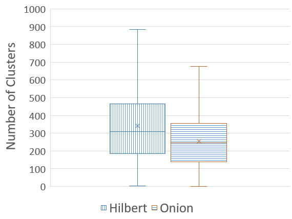
The box plot of distributions of clustering numbers from the onion and Hilbert curves over $Q_{\rho}$ is shown in Figure 6 for $d=2$ and Figure 6 for $d=3$ respectively. From these results, we observe that the median performance of the onion curve is better than the Hilbert curve in all cases that were considered. The difference in performance was the greatest when the ratio of side lengths approaches $1$ (i.e. the shape gets closer to a square).

Algorithm 1 Generate a set

Q_{\rho}

of random rectangles with a fixed side length ratio

\rho

with

d=2

Initialize

\sqrt{n}=\ell_{2}=\sqrt{n},~Q_{\rho}=\emptyset

1 while $\ell_{2}\geq 0$ do

2 Set

\ell_{1}=\lfloor\ell_{2}/\rho\rfloor

3 if $\ell_{1}\leq\sqrt{n}$ then

4 for $i=1,2,\cdots,20$ do

5 Sample

x

and

y

independnetly from

\mathcal{U}(\sqrt{n}-\ell_{1})

and

\mathcal{U}(\sqrt{n}-\ell_{2})

Q_{\rho}\leftarrow Q_{\rho}\cup\{\mathsf{L}(x,y,\ell_{1},\ell_{2})\}

\ell_{2}\leftarrow\ell_{2}-50

VII-C Rectangular Queries, Random End Points

In this experiment we generate a set of rectangles with random corner points. For an integer $N$ , let $\mathcal{U}(N)$ denote the uniform distribution over $\{0,1,2,\ldots,N\}$ . For the case $d=2$ , we generate a set $Q$ of rectangles by choosing the two corners of the rectangle uniformly at random, and then considering the smallest rectangle that contains both the chosen points. We generated rectangles chosen in a similar random manner, for the case $d=3$ . The box plot of distributions of clustering numbers from the onion and Hilbert curves over $Q$ is shown in Figure 7 for $d=2$ and Figure 7 for $d=3$ respectively.

VIII Conclusions

We presented a new SFC, the onion curve, in two and three dimensions. This is the first SFC we know of, whose clustering performance is within a constant factor of the optimal for all cube and near-cube query sets. In contrast, the clustering performance of the Hilbert curve can be far from optimal. Further, the clustering performance of the onion curve is no worse that the Hilbert curve in all cases considered. The definition of the onion curve is simple, making it easy to use.

However, we note that our analysis does not mean that the onion curve is unambiguously better than other curves, say, the Hilbert curve, in terms of organizing data for say range queries. There are other aspects of clustering that we have not analyzed here, for example, the distance between different clusters of the same query region, which tends to be important in fetching data from the disk. Such an analysis is interesting and the subject of future work.

The onion curve can be extended naturally to higher dimensions, using the idea of ordering points according to increasing distance from the edge of the universe. The analysis of such a higher dimensional onion curve is the subject of future work. It is also interesting to consider the performance of Hilbert curve for general near-cube query sets as we do for the onion curve. Another future work is to complete Table II by filling the missing results for the Hilbert curve for general near-cube query sets.

IX Acknowledgments

The research of the first author is supported in part by NSF Awards CNS 1010789 and CCF 1422569.

References

[1] J. A. Orenstein and T. H. Merrett, “A class of data structures for associative searching,” in Proceedings of the 3rd ACM SIGACT-SIGMOD symposium on Principles of database systems, ser. PODS ’84, 1984, pp. 181–190.
[2] H. V. Jagadish, “Linear clustering of objects with multiple attributes,” in Proceedings of the 1990 ACM SIGMOD international conference on Management of data, ser. SIGMOD ’90, 1990, pp. 332–342.
[3] K. Aydin, M. Bateni, and V. Mirrokni, “Distributed balanced partitioning via linear embedding,” in Proc. of the Ninth ACM International Conference on Web Search and Data Mining (WSDM), 2016, pp. 387–396.
[4] M. Warren and J. Salmon, “A parallel hashed-octtree N-body algorithm,” in Proceedings of Supercomputing ’93, Portland, OR, Nov. 1993.
[5] T. Li, Y. Lin, and H. Shen, “A locality-aware similar information searching scheme,” Int. J. on Digital Libraries, vol. 17, no. 2, pp. 79–93, 2016.
[6] H. Liu, K. Wang, B. Yang, M. Yang, R. He, L. Shen, H. Zhong, and Z. Chen, “Load balancing using hilbert space-filling curves for parallel reservoir simulations,” CoRR, vol. abs/1708.01365, 2017. [Online]. Available: http://arxiv.org/abs/1708.01365
[7] H. Kim, S. Hong, and J. Chang, “Hilbert curve-based cryptographic transformation scheme for spatial query processing on outsourced private data,” Data Knowl. Eng., vol. 104, pp. 32–44, 2016.
[8] C. Faloutsos, “Multiattribute hashing using gray codes,” SIGMOD Record, vol. 15, pp. 227–238, June 1986.
[9] ——, “Gray codes for partial match and range queries,” IEEE Trans. Software Engg., vol. 14, pp. 1381–1393, 1988.
[10] D. Hilbert, “Über die stetige Abbildung einer Linie auf ein Flächenstück,” Math. Ann., vol. 38, pp. 459–460, 1891.
[11] B. Moon, H. V. Jagadish, C. Faloutsos, and J. H. Saltz, “Analysis of the clustering properties of the Hilbert space-filling curve,” IEEE Trans. Knowledge and Data Engineering, vol. 13, no. 1, pp. 124–141, 2001.
[12] H. V. Jagadish, “Analysis of the Hilbert curve for representing two-dimensional space,” Information Processing Letters, vol. 62, pp. 17–22, 1997.
[13] P. Xu and S. Tirthapura, “Optimality of clustering properties of space-filling curves,” ACM Transactions on Database Systems (TODS), vol. 39, no. 2, p. 10, 2014.
[14] C. Gotsman and M. Lindenbaum, “On the metric properties of discrete space-filling curves,” IEEE Trans. Image Processing, vol. 5, no. 5, pp. 794–797, 1996.
[15] T. Asano, D. Ranjan, T. Roos, E. Welzl, and P. Widmayer, “Space-filling curves and their use in the design of geometric data structures,” Theor. Comput. Sci., vol. 181, no. 1, pp. 3–15, 1997.
[16] H. J. Haverkort, “Recursive tilings and space-filling curves with little fragmentation,” Journal of Computational Geometry, vol. 2, no. 1, pp. 92–127, 2011.
[17] J. Alber and R. Niedermeier, “On Multidimensional Curves with Hilbert Property,” Theory Comput. Syst., vol. 33, no. 4, pp. 295–312, 2000.
[18] P. Xu and S. Tirthapura, “On the optimality of clustering properties of space filling curves,” in Proceedings of the 31st ACM Symposium on Principles of Database Systems, PODS, 2012, pp. 215–224.

Onion Curve: A Space Filling Curve with Near-Optimal Clustering

Abstract

I Introduction

Model

I-A Our Results

I-B Related Work

II General Techniques

Lemma 1

Proof:

III Onion Curve in Two Dimensions

III-A Onion Curve Definition

III-B Clustering Number of Onion Curve in Two Dimensions for Rectangular Queries

Theorem 1

III-B1 Computing γ⁡(Q,π)\gamma(Q,\pi) in Two Dimensions for an SFC π\pi

Lemma 2

Proof:

III-B2 Clustering Number of the Onion Curve

Lemma 3

Proof:

Lemma 4

Proof:

Proof:

IV Clustering Number of the Hilbert Curve

Lemma 5

Proof:

V Lower Bound in Two Dimensions

V-A Lower Bound for Continuous SFCs

Definition 1

Theorem 2

Definition 2

Lemma 6

Proof:

Lemma 7

Lemma 8

Proof:

V-B Lower Bound for General SFCs

Theorem 3

Definition 3

Lemma 9

Proof:

V-C General Rectangular Query Sets

Lemma 10

Proof:

Lemma 11

V-D Approximation Ratios of the Onion Curve and the Hilbert Curve for Near Cube Queries

VI Three-dimensional Onion Curve

VI-A Definition of the Onion Curve in Three Dimensions

VI-B Upper and Lower Bounds

Theorem 4

Theorem 5

Theorem 6

VI-C Discussion on the Three-dimensional Onion Curve

VII Experimental Study

VII-A Clustering Performance on Cube Queries

VII-B Rectangular Queries, Fixed Ratio of Side Lengths

VII-C Rectangular Queries, Random End Points

VIII Conclusions

IX Acknowledgments

References

III-B1 Computing $\gamma(Q,\pi)$ in Two Dimensions for an SFC $\pi$