1Introduction

BHS: Böhm, Hollik ans Spiesberger
BSM: Beyond the Standard Model
CKM: Cabibbo $-$ Kobayashi $-$ Maskawa
CT: counterterm
EW: electroweak
FCNC: flavour-changing neutral currents
HXSWG: LHC Higgs Cross Section Working Group
IR: Infrared
LHC: Large Hadron Collider
LO: leading order
MS: Minimal Subtraction
NLO: next-to-leading order
OS: on-shell
PDG: Particle Data Group
QCD: quantum chromodynamics
RGE: renormalization group equation
SB: symmetry breaking
SM: Standard Model
SESM: Singlet Extension of the Standard Model
THDM: Two-Higgs-Doublet Model
UV: ultraviolet
vev: vacuum expectation value

FR-PHENO-2017-024

Precision calculations for $\text{h}\to\text{W}\text{W}/\text{Z}\text{Z}\to 4$ fermions
in a Singlet Extension of the Standard Model with Prophecy4f

Lukas Altenkamp, Michele Boggia and Stefan Dittmaier
Albert-Ludwigs-Universität Freiburg, Physikalisches Institut,
79104 Freiburg, Germany

Abstract:

We consider an extension of the Standard Model by a real singlet scalar field with a $\mathbb{Z}_{2}$ -symmetric Lagrangian and spontaneous symmetry breaking with vacuum expectation value for the singlet. Considering the lighter of the two scalars of the theory to be the $125\,\,\mathrm{GeV}$ Higgs particle, we parametrize the scalar sector by the mass of the heavy Higgs boson, a mixing angle $\alpha$ , and a scalar Higgs self-coupling $\lambda_{12}$ . Taking into account theoretical constraints from perturbativity and vacuum stability, we compute next-to-leading-order electroweak and QCD corrections to the decays $\text{h}\to\text{W}\text{W}/\text{Z}\text{Z}\to 4\,$ fermions of the light Higgs boson for some scenarios proposed in the literature. We formulate two renormalization schemes and investigate the conversion of the input parameters between the schemes, finding sizeable effects. Solving the renormalization-group equations for the $\overline{\text{MS}}$ parameters $\alpha$ and $\lambda_{12}$ , we observe a significantly reduced scale and scheme dependence in the next-to-leading-order results. For some scenarios suggested in the literature, the total decay width for the process $\text{h}\to 4f$ is computed as a function of the mixing angle and compared to the width of a corresponding Standard Model Higgs boson, revealing deviations below $10\%$ . Differential distributions do not show significant distortions by effects beyond the Standard Model. The calculations are implemented in the Monte Carlo generator Prophecy4f, which is ready for applications in data analyses in the framework of the singlet extension.

January 2018

1 Introduction

The discovery of a Higgs boson [1, 2] at Run 1 of the LHC (LHC) was a milestone in the experimental exploration of EW (EW) interaction. Precision studies of the Higgs particle are now needed in order to further explore the nature of the EW symmetry breaking mechanism. Measurements from the ATLAS and CMS collaborations at LHC Runs 1 and 2 are compatible, within the current accuracy, with the SM (SM), in which the symmetry breaking is modeled by the Higgs mechanism and driven by an $\text{SU}(2)_{\scriptscriptstyle\text{W}}$ scalar doublet in the Lagrangian. Since there are observed phenomena that cannot be explained within the standard framework, such as the existence of dark matter, massive neutrinos, and the baryonic asymmetry of the universe, we believe that the SM is not the ultimate theory. The hope is to observe deviations from the SM in the next years of data taking at the LHC, as experimental uncertainties will decrease with increasing luminosity. In case deviations will show up, theoretical predictions at the highest possible accuracy will be required for physics BSM (BSM) in order to properly confront predictions with the experimental findings. If new resonances are observed, precise predictions within BSM theories will be necessary in order to find out to which model extensions they might belong. In case no new particles are found, experimental and theoretical accuracy will help to test the viability of BSM theories as well.

Several strategies were proposed to make steps towards the next SM (see e.g. the reviews [3, 4] and references therein), which includes the study of specific models, the use of effective field theories based on the SM gauge group, and simplified models. Among these, Higgs sector extensions are of particular interest, as these can be considered both as complete $\text{SU}(2)_{\scriptscriptstyle\text{W}}\times\text{U}(1)_{\scriptscriptstyle\text{Y}}$ symmetric models (featuring a non-minimal EW symmetry breaking mechanism) and as simplified models (where additional scalars can interact with hypothetical BSM sectors). The simplest way to enlarge the SM Higgs sector is by adding a gauge-singlet field, which is neutral under the gauge symmetry of the SM. This extension, despite its simplicity, can provide interesting phenomenology. It was initially proposed by Silveira and Zee to motivate the presence of dark matter [5] and introduced—in different variants—in Refs. [6, 7] to analyze the high-energy and the heavy-Higgs-mass limits as well as the (non-)decoupling properties in radiative corrections to the self-interactions of W bosons.

The key feature of this extension is that the additional field interacts with SM matter only through couplings to the $\text{SU}(2)_{\scriptscriptstyle\text{W}}$ Higgs doublet. The form of the Lagrangian is determined by requiring gauge invariance, renormalizability, and optional extra symmetries. Different scenarios can be realized with a zero or a non-vanishing vev (vev) for the singlet field, which could be real or complex. Under certain conditions, the additional scalar provides the “Higgs portal” for a dark matter candidate or is a dark-matter candidate itself, as discussed in Refs. [5, 8, 9, 10, 11, 12, 13, 14, 15, 16, 17, 18, 19, 20, 21, 22, 23]. On the other hand, the additional singlet might act as initiator of a first-order EW phase transition [24, 25, 26]. The interesting phenomenology of SESM influenced search strategies for the Higgs boson (and vice versa) already before the Higgs-boson discovery (see, e.g., Refs. [27, 28, 29, 22, 30]); nowadays data from EW precision physics, LHC Higgs measurements, and dark matter searches lead to strong constraints on SESM [31, 32, 33, 34, 35, 36, 37, 38].

We consider the most simple variant of a SESM which comprises one real singlet field with a $\mathbb{Z}_{2}$ -symmetric Lagrangian in the unbroken phase and assign a non-vanishing vev to the gauge singlet. The non-vanishing vev leads to mixing between the singlet scalar and the Higgs boson contained in the $\text{SU}(2)_{\scriptscriptstyle\text{W}}$ doublet, a feature that is quite generic in more comprehensive SM extensions, which renders this SESM variant a very useful prototype for a simplified model. In comparison to that, the SESM with a vanishing vev is phenomenologically less interesting and will, therefore, not be considered in this paper. In the SESM, the single CP-even Higgs boson of the SM is replaced by two CP-even Higgs bosons. The SM coupling strength is shared by the two Higgs bosons, i.e. the Higgs bosons couple with the SM strength weighted by the sine or cosine of a mixing angle. The mass of the additional Higgs boson, the Higgs mixing angle, and one coupling factor of the scalar self-interactions parametrize the extended sector. In our phenomenological study, the lightest of the two Higgs bosons of the theory is considered to be the $125\,\,\mathrm{GeV}$ resonance observed at the LHC, but our theoretical approach is not restricted to this case.

Our goal is to perform NLO (NLO) computations within the SESM, including both EW and QCD (QCD) corrections. To this end, it is necessary to renormalize the theory. Recently, the renormalization of SM extensions has been subject of discussion, since very often there is no obvious formulation of OS (OS) renormalization conditions to define BSM parameters that are fully based on physical S-matrix elements. To define these parameters, it is customary to use renormalization conditions in the modified Minimal Subtraction ( $\overline{\text{MS}}$ ) scheme. While a consistent use of OS conditions based on physical S-matrix elements guarantees a gauge-independent parametrization of physical observables by renormalized input parameters, making use of both OS and $\overline{\text{MS}}$ conditions in the definition of a renormalization scheme can lead to gauge-dependent renormalization constants if the (gauge-dependent) tadpoles are not treated properly. In Ref. [39], Fleischer and Jegerlehner proposed a renormalization scheme to avoid this problem in the SM, followed by other approaches such as, e.g., described in Ref. [40]. Recently, these strategies have been applied to THDM in Refs. [41, 42, 43, 44].

Different renormalization schemes for the SESM with a real singlet scalar were already considered in Refs. [45, 46, 47, 48, 44]. Among these proposals there is no convincing scheme that is fully based on OS conditions. Most schemes are based on ad hoc or on $\overline{\text{MS}}$ conditions, and many variants still suffer from gauge dependence issues. In this paper, we build on OS conditions as far as possible and take $\overline{\text{MS}}$ conditions for those parameters for which no distinguished OS conditions are available.¹¹ 1 In our work we do not consider schemes based on the “pinch technique”, as, e.g., suggested in Ref. [48]. Following the arguments of Refs. [49, 50] we consider the “pinch technique” just as one of many physically equivalent choices to fix the gauge arbitrariness in off-shell quantities (related to the ’t Hooft–Feynman gauge of the quantum fields in the background-field gauge) rather than singling out “its gauge-invariant part” in any sense. We formulate two renormalization schemes for the SESM, using two different ways to treat tadpole contributions, one of them based on the FJ variant [39], similar to a proposal made in Ref. [44]. We analyze, in both cases, the dependence of our NLO results on the renormalization scale $\mu_{\text{r}}$ , which is due to $\overline{\text{MS}}$ definitions of the Higgs mixing angle and the Higgs self-coupling $\lambda_{12}$ . We study the conversion of input parameters between the two schemes and compare the results obtained in the two schemes to inspect the perturbative consistency of the chosen region for $\mu_{\text{r}}$ . Parameter conversions between different renormalization schemes, and the corresponding scheme dependence of NLO results, were not yet discussed for the previously proposed schemes and their applications. In a situation where no distinguished renormalization scheme has yet emerged, discussions of renormalization scale and renormalization scheme dependences are very important in applications.

In this work, we compute decay observables for the decays of the $125\,\,\mathrm{GeV}$ Higgs boson of the SESM into four fermions via intermediate (off-shell) WW or ZZ states. These processes played a central role in the discovery of the Higgs boson, and are very important channels in Higgs couplings analyses. NLO computations for these processes were performed, including both EW and QCD corrections, in the SM with the Monte Carlo generator Prophecy4f [51, 52, 53] (and matched to a QED parton shower in Ref. [54]), as well as in presence of a fourth fermion generation [55] and in the THDM [44, 56], but there are no corresponding results available yet in the SESM.

Using the Mathematica package FeynRules [57, 58], we have implemented the Feynman rules for the SESM into a FeynArts [59] model file, which includes one-loop CT for both renormalization schemes. The model file has been used to compute, with the Mathematica package FormCalc [60], the matrix elements for the decays of the light Higgs into four fermions (including EW and QCD NLO corrections) and to produce Fortran routines to extend the Monte Carlo program Prophecy4f. Finally, we have used the extended Prophecy4f version to compute partial widths and to generate differential distributions for a selection of benchmark scenarios, proposed in Refs. [37, 3]. Other computations of NLO EW corrections relevant for phenomenology in SESM can be found in Refs. [46, 45, 47, 48, 44].

The paper is organized as follows. In Sect. 2, we describe the Lagrangian of the SESM considered in this work and discuss the basic features of the model. We set up the renormalization procedure introducing renormalization transformations for fields and parameters in Sect. 3 and fixing the renormalization constants in Sect. 4. In Sect. 5, we briefly describe the capabilities of the Monte Carlo program Prophecy4f and discuss the computation of decay observables for the processes $\text{h}\to\text{W}\text{W}/\text{Z}\text{Z}\to 4\,$ fermions. In Sect. 6, we provide the input parameters and discuss the benchmark scenarios used to produce the numerical results shown in Sect. 7. In Sect. 8 we draw our conclusions. Additional numerical results are reported in the appendices.

2 Singlet Extension of the Standard Model

Singlet extensions of the SM add one or more scalar singlet fields to the SM Higgs sector. In general, the scalar fields can be complex, but we here consider the simplest variant of a SESM with one additional real field. The Lagrangian of the model can be easily obtained by modifying the scalar sector of the SM. As the extension does not modify strong interactions, we present only the contributions to the total SESM Lagrangian that are relevant for the EW sector, while the QCD part can be taken over from any standard reference, such as Ref. [61]. For convenience, we split the EW Lagrangian of the model as follows:

{\cal L}_{\text{SESM}}={\cal L}_{\text{Gauge}}+{\cal L}_{\text{Fermion}}+{\cal L}_{\text{Higgs}}+{\cal L}_{\text{Yukawa}}+{\cal L}_{\text{Fix}}+{\cal L}_{\text{Ghost}}.

(2.1)

By gauge symmetry and renormalizability constraints, only small deviations from the SM are allowed: The additional scalar field, which has mass dimension 1 and is neutral under $\text{SU}(2)_{\scriptscriptstyle\text{W}}\times\text{U}(1)_{\scriptscriptstyle\text{Y}}$ gauge transformations, can be coupled to the SM fields only through gauge-invariant terms with mass dimension of at most 3, i.e. the singlet scalar can only couple to $\Phi^{\dagger}\Phi$ , with $\Phi$ denoting the SM-like Higgs doublet. Moreover, the Higgs Lagrangian contains a kinetic term and self-interaction terms of the singlet field in addition to the terms that are already present in the SM. Since the singlet enters only the Higgs Lagrangian ${\cal L}_{\text{Higgs}}$ , the gauge, fermionic, Yukawa, gauge-fixing, and ghost terms of Eq. 2.1 only need little adaption from the SM. For these contributions we make use of the formulation of Ref. [62]. In Sect. 2.1 we introduce the conventions used for the Higgs Lagrangian, then we briefly discuss the gauge (Sect. 2.2) and the fermion sectors (Sect. 2.3). Finally, we define our input parameter set in Sect. 2.4.

2.1 Higgs Lagrangian

2.1.1 Mass spectrum

In complex SESM, the singlet field is supposed to be responsible for the symmetry breaking in a hypothetical hidden sector, where interactions of the hidden sector are governed by an exotic $\text{U}(1)$ or even higher-rank gauge symmetry [12, 14, 18, 32, 34]. Considering our SESM as a downgrade of such a more comprehensive theory which still carries salient features of the more complete theory, we enforce a $\mathbb{Z}_{2}$ symmetry on the Higgs Lagrangian (under sign change of the singlet field). Moreover, we require a non-vanishing vev for the singlet. The model obtained in this way is very simple, but still phenomenologically interesting, as it involves mixing of the new singlet scalar with the Higgs field of the SM scalar sector, which is a generic feature of many SM extensions. The most general renormalizable, gauge- and $\mathbb{Z}_{2}$ -invariant Higgs Lagrangian in presence of one real singlet and one doublet is given by [17, 28]

\begin{split}{\cal L}_{\text{Higgs}}&={\cal L}_{\text{Higgs,kin}}-V(\Phi,\sigma),\\ {\cal L}_{\text{Higgs,kin}}&=(D_{\mu}\Phi)^{\dagger}(D^{\mu}\Phi)+\frac{1}{2}(\partial_{\mu}\sigma)(\partial^{\mu}\sigma),\\ V(\Phi,\sigma)&=-\mu_{2}^{2}\Phi^{\dagger}\Phi+\frac{\lambda_{2}}{4}(\Phi^{\dagger}\Phi)^{2}+\lambda_{12}\sigma^{2}\Phi^{\dagger}\Phi-\mu_{1}^{2}\sigma^{2}+\lambda_{1}\sigma^{4},\end{split}

(2.2)

where $\Phi$ is the complex SM scalar doublet with hypercharge $Y_{{\scriptscriptstyle\text{W}},\Phi}=1$ , and $\sigma$ is the real singlet field. Splitting off the vev $v_{2}$ and $v_{1}$ , we parametrize $\Phi$ and $\sigma$ by

\Phi=\begin{pmatrix}\phi^{+}\\ \frac{1}{\sqrt{2}}(v_{2}+h_{2}+\mathrm{i}\chi)\end{pmatrix},\quad\sigma=v_{1}+h_{1},

(2.3)

where $\phi^{+}$ , $\phi^{-}=(\phi^{+})^{\dagger}$ , and $\chi$ denote the would-be Goldstone-boson fields for the $\text{W}^{\pm}$ and Z bosons. The covariant derivative, which is relevant for the couplings of $\Phi$ to the EW gauge bosons, is given by

D_{\mu}=\partial_{\mu}{-\mathrm{i}g_{2}I_{\scriptscriptstyle\text{W}}^{a}W_{\mu}^{a}}+\mathrm{i}g_{1}\frac{Y_{\scriptscriptstyle\text{W}}}{2}B_{\mu}.

(2.4)

In Eq. 2.4, $g_{2}$ , $I_{\scriptscriptstyle\text{W}}^{a}$ ( $a=1,2,3$ ), and $W_{\mu}^{a}$ are, respectively, the gauge coupling, the generators, and the gauge fields of the weak isospin $\text{SU}(2)_{\scriptscriptstyle\text{W}}$ group; $g_{1}$ , $Y_{\scriptscriptstyle\text{W}}$ , and $B_{\mu}$ are the gauge coupling, the generator, and gauge field of the weak hypercharge $\text{U}(1)_{\scriptscriptstyle\text{Y}}$ group.²² 2 The negative sign in the $\text{SU}(2)_{\scriptscriptstyle\text{W}}$ term of the covariant derivative $D_{\mu}$ is used by Böhm, Hollik and Spiesberger [63], while a positive sign is, e.g., used by Gunion, Haber, Kane and Dawson [64]. We make use of the former by default, but in our implementations both conventions are supported. For convenience, in Eq. 2.3, we introduce the subscripts $1$ and $2$ to label vev and fields for the singlet and the doublet sectors, respectively. The role of $v_{2}$ is the same as in the SM, since only $\Phi$ couples to the EW gauge bosons. The vev of the singlet, $v_{1}$ , can be vanishing or non-vanishing, providing different phenomenology. As stated before, we consider the case $v_{1}\neq 0$ , which is phenomenologically more interesting. Two non-vanishing vev can only arise for $\mu_{2}^{2},\mu_{1}^{2}>0$ and if the following vacuum stability conditions are fulfilled,

\lambda_{2}>0,\quad\lambda_{1}>0,\quad\lambda_{2}\lambda_{1}-\lambda_{12}^{2}>0.

(2.5)

Expanding the potential $V$ with the decomposition (2.3) and keeping terms containing the fields $h_{2},h_{1}$ up to second order leads to

V_{2}=-t_{2}h_{2}-t_{1}h_{1}+\frac{1}{2}\begin{pmatrix}h_{2},h_{1}\end{pmatrix}{\cal M}^{2}_{\text{Higgs}}\begin{pmatrix}h_{2}\\ h_{1}\end{pmatrix},

(2.6)

with the tadpole parameters

t_{2}=\frac{v_{2}}{4}\left(4\mu_{2}^{2}-4v_{1}^{2}\lambda_{12}-v_{2}^{2}\lambda_{2}\right),\qquad t_{1}=v_{1}\left(2\mu_{1}^{2}-v_{2}^{2}\lambda_{12}-4v_{1}^{2}\lambda_{1}\right),

(2.7)

and the non-diagonal mass matrix

{\cal M}^{2}_{\text{Higgs}}=\begin{pmatrix}v_{1}^{2}\lambda_{12}+\frac{3v_{2}^{2}\lambda_{2}}{4}-\mu_{2}^{2}&2v_{1}v_{2}\lambda_{12}\\ 2v_{1}v_{2}\lambda_{12}&v_{2}^{2}\lambda_{12}+12v_{1}^{2}\lambda_{1}-2\mu_{1}^{2}\end{pmatrix}.

(2.8)

In order to work with fields related to mass eigenstates, we diagonalize the mass matrix by a rotation about an angle $\alpha$ with $-\pi/2\leq\alpha\leq\pi/2$ ,

\begin{pmatrix}h\\ H\end{pmatrix}=\begin{pmatrix}c_{\alpha}&-s_{\alpha}\\ s_{\alpha}&c_{\alpha}\end{pmatrix}\begin{pmatrix}h_{2}\\ h_{1}\end{pmatrix},

(2.9)

using the abbreviations $c_{\alpha}\equiv\cos\alpha$ and $s_{\alpha}\equiv\sin\alpha$ . The potential (up to second power in $h,H$ ) takes the form

V_{2}=-t_{\text{h}}h-t_{\text{H}}H+\frac{1}{2}\begin{pmatrix}h,H\end{pmatrix}\widetilde{{\cal M}}^{2}_{\text{Higgs}}\begin{pmatrix}h\\ H\end{pmatrix},

(2.10)

with the tadpole parameters $t_{\text{h}},t_{\text{H}}$ for the fields $h$ and $H$ given by

t_{\text{h}}=c_{\alpha}t_{2}-s_{\alpha}t_{1},\qquad t_{\text{H}}=s_{\alpha}t_{2}+c_{\alpha}t_{1}.

(2.11)

Diagonalizing $\widetilde{{\cal M}}^{2}_{\text{Higgs}}$ fixes the mixing angle by

\begin{split}\cos(2\alpha)&=\pm\frac{16v_{1}^{2}\lambda_{1}-v_{2}^{2}\lambda_{2}}{\sqrt{\left(8v_{1}v_{2}\lambda_{12}\right)^{2}+\left(16v_{1}^{2}\lambda_{1}-v_{2}^{2}\lambda_{2}\right)^{2}}},\\ \sin(2\alpha)&=\pm\frac{8v_{1}v_{2}\lambda_{12}}{\sqrt{\left(8v_{1}v_{2}\lambda_{12}\right)^{2}+\left(16v_{1}^{2}\lambda_{1}-v_{2}^{2}\lambda_{2}\right)^{2}}},\end{split}

(2.12)

with eigenvalues

\begin{split}M_{\text{h}}^{2}&=\frac{1}{2}\lambda_{2}v_{2}^{2}-2\lambda_{12}v_{1}v_{2}t_{\alpha},\\ M_{\text{H}}^{2}&=\frac{1}{2}\lambda_{2}v_{2}^{2}+\frac{2\lambda_{12}v_{1}v_{2}}{t_{\alpha}},\end{split}

(2.13)

where $t_{\alpha}\equiv s_{\alpha}/c_{\alpha}$ is the tangent of the mixing angle. We choose the upper sign in (2.12) to enforce the hierarchy $M_{\text{h}}<M_{\text{H}}$ of the two Higgs-boson masses, i.e. we take $0<\alpha<\frac{\pi}{2}$ if $\lambda_{12}$ is positive or $-\frac{\pi}{2}<\alpha<0$ if $\lambda_{12}$ is negative. The squared Higgs-boson masses, which are equal to the eigenvalues of $\widetilde{{\cal M}}^{2}_{\text{Higgs}}$ , can be written as

\begin{split}M_{\text{h}}^{2}&=\frac{1}{4}v_{2}^{2}\lambda_{2}+4v_{1}^{2}\lambda_{1}-\frac{1}{4}\sqrt{\left(8v_{1}v_{2}\lambda_{12}\right)^{2}+\left(16v_{1}^{2}\lambda_{1}-v_{2}^{2}\lambda_{2}\right)^{2}},\\ M_{\text{H}}^{2}&=\frac{1}{4}v_{2}^{2}\lambda_{2}+4v_{1}^{2}\lambda_{1}+\frac{1}{4}\sqrt{\left(8v_{1}v_{2}\lambda_{12}\right)^{2}+\left(16v_{1}^{2}\lambda_{1}-v_{2}^{2}\lambda_{2}\right)^{2}}.\end{split}

(2.14)

We express the original parameters $\mu_{2}^{2},\mu_{1}^{2},\lambda_{2},\lambda_{1},\lambda_{12}$ in terms of the physical masses $M_{\text{h}},M_{\text{H}}$ , the mixing angle $\alpha$ , the vev $v_{2}$ , and the dimensionless coupling $\lambda_{12}$ , in order to have five free parameters that are more suited as phenomenological input. Note that the vev $v_{2}$ is fixed by EW symmetry breaking (see Sect. 2.2). To derive the Lagrangian and the Feynman rules, we express all original parameters of the Higgs potential in terms of the new ones. In detail, we solve the equations $t_{2}=t_{1}=0$ (see Eq. 2.7) and Eqs. (2.12), (2.14) for the original Higgs parameters, resulting in

\begin{split}v_{1}&=\frac{s_{2\alpha}\left(M_{\text{H}}^{2}-M_{\text{h}}^{2}\right)}{4v_{2}\lambda_{12}},\\ \mu_{2}^{2}&=\frac{1}{2}\left(c_{\alpha}^{2}M_{\text{h}}^{2}+s_{\alpha}^{2}M_{\text{H}}^{2}\right)+\frac{s_{2\alpha}^{2}\left(M_{\text{H}}^{2}-M_{\text{h}}^{2}\right)^{2}}{16\lambda_{12}v_{2}^{2}},\\ \mu_{1}^{2}&=\frac{1}{4}\left(c_{\alpha}^{2}M_{\text{H}}^{2}+s_{\alpha}^{2}M_{\text{h}}^{2}\right)+\frac{1}{2}\lambda_{12}v_{2}^{2},\\ \lambda_{2}&=\frac{2\left(c_{\alpha}^{2}M_{\text{h}}^{2}+s_{\alpha}^{2}M_{\text{H}}^{2}\right)}{v_{2}^{2}},\\ \lambda_{1}&=\frac{2\left(c_{\alpha}^{2}M_{\text{H}}^{2}+s_{\alpha}^{2}M_{\text{h}}^{2}\right)\lambda_{12}^{2}v_{2}^{2}}{s_{2\alpha}^{2}\left(M_{\text{H}}^{2}-M_{\text{h}}^{2}\right)^{2}},\end{split}

(2.15)

where the shorthand notations $s_{n\alpha}\equiv\sin\left(n\alpha\right),c_{n\alpha}\equiv\cos\left(n\alpha\right)$ are used. Using the parameterization (2.15), the vacuum stability conditions (2.5) are automatically fulfilled, while $\mu_{2}^{2}>0$ and $\mu_{1}^{2}>0$ lead to a restriction on the parameter space of the theory by

\lambda_{12}>0\quad\text{or}\quad-\frac{c_{\alpha}^{2}M_{\text{H}}^{2}+s_{\alpha}^{2}M_{\text{h}}^{2}}{2v_{2}^{2}}<\lambda_{12}<-\frac{s_{2\alpha}^{2}(M_{\text{H}}^{2}-M_{\text{h}}^{2})^{2}}{8v_{2}^{2}(c_{\alpha}^{2}M_{\text{h}}^{2}+s_{\alpha}^{2}M_{\text{H}}^{2})}.

(2.16)

2.1.2 Couplings

We insert the expressions (2.3) and (2.9) as well as Eq. 2.7 with $t_{2}=t_{1}=0$ into the potential of Eq. 2.2 obtaining

\begin{split}V&=\text{const.}+\frac{1}{2}M_{\text{h}}^{2}h^{2}+\frac{1}{2}M_{\text{H}}^{2}H^{2}+c_{\text{h}\text{h}\text{h}}h^{3}+c_{\text{h}\text{h}\text{H}}h^{2}H+c_{\text{h}\text{H}\text{H}}hH^{2}+c_{\text{H}\text{H}\text{H}}H^{3}\\ &\quad+c_{\text{h}\text{h}\text{h}\text{h}}h^{4}+c_{\text{h}\text{h}\text{h}\text{H}}h^{3}H+c_{\text{h}\text{h}\text{H}\text{H}}h^{2}H^{2}+c_{\text{h}\text{H}\text{H}\text{H}}hH^{3}+c_{\text{H}\text{H}\text{H}\text{H}}H^{4}\\ &\quad+\frac{1}{2}\left[c_{\text{h}\phi\phi}h+c_{\text{H}\phi\phi}H+c_{\text{h}\text{h}\phi\phi}h^{2}+c_{\text{h}\text{H}\phi\phi}hH+c_{\text{H}\text{H}\phi\phi}H^{2}\right]\left(2\phi^{+}\phi^{-}+\chi^{2}\right)\\ &\quad+\frac{\lambda_{2}}{16}\left(2\phi^{+}\phi^{-}+\chi^{2}\right)^{2},\end{split}

(2.17)

with the coupling constants given by

$\displaystyle c_{\text{h}\text{h}\text{h}}$	$\displaystyle=\frac{c_{\alpha}^{3}}{4}\lambda_{2}v_{2}+\frac{s_{2\alpha}}{2}\lambda_{12}\left(s_{\alpha}v_{2}-c_{\alpha}v_{1}\right)-4s_{\alpha}^{3}\lambda_{1}v_{1},$
$\displaystyle c_{\text{h}\text{h}\text{H}}$	$\displaystyle=\frac{3c_{\alpha}s_{2\alpha}}{8}\lambda_{2}v_{2}+\lambda_{12}\left[s_{\alpha}\left(-2c_{\alpha}^{2}+s_{\alpha}^{2}\right)v_{2}+c_{\alpha}\left(c_{\alpha}^{2}-2s_{\alpha}^{2}\right)v_{1}\right]+6s_{\alpha}s_{2\alpha}\lambda_{1}v_{1},$
$\displaystyle c_{\text{h}\text{H}\text{H}}$	$\displaystyle=\frac{3s_{\alpha}s_{2\alpha}}{8}\lambda_{2}v_{2}+\lambda_{12}\left[c_{\alpha}\left(c_{\alpha}^{2}-2s_{\alpha}^{2}\right)v_{2}+s_{\alpha}\left(2c_{\alpha}^{2}-s_{\alpha}^{2}\right)v_{1}\right]-6c_{\alpha}s_{2\alpha}\lambda_{1}v_{1},$
$\displaystyle c_{\text{H}\text{H}\text{H}}$	$\displaystyle=\frac{s_{\alpha}^{3}}{4}\lambda_{2}v_{2}+\frac{s_{2\alpha}}{2}\lambda_{12}\left(c_{\alpha}v_{2}+s_{\alpha}v_{1}\right)+4c_{\alpha}^{3}\lambda_{1}v_{1},$
$\displaystyle c_{\text{h}\text{h}\text{h}\text{h}}$	$\displaystyle=\frac{c_{\alpha}^{4}}{16}\lambda_{2}+\frac{s_{2\alpha}^{2}}{8}\lambda_{12}+s_{\alpha}^{4}\lambda_{1},$
$\displaystyle c_{\text{h}\text{h}\text{h}\text{H}}$	$\displaystyle=\frac{c_{\alpha}^{2}s_{2\alpha}}{8}\lambda_{2}-\frac{c_{2\alpha}s_{2\alpha}}{2}\lambda_{12}-2s_{\alpha}^{2}s_{2\alpha}\lambda_{1},$
$\displaystyle c_{\text{h}\text{h}\text{H}\text{H}}$	$\displaystyle=\frac{3s_{2\alpha}^{2}}{32}\lambda_{2}+\frac{2c_{2\alpha}^{2}-s_{2\alpha}^{2}}{4}\lambda_{12}+\frac{3s_{2\alpha}^{2}}{2}\lambda_{1},$	(2.18)
$\displaystyle c_{\text{h}\text{H}\text{H}\text{H}}$	$\displaystyle=\frac{s_{2\alpha}s_{\alpha}^{2}}{8}\lambda_{2}+\frac{c_{2\alpha}s_{2\alpha}}{2}\lambda_{12}-2c_{\alpha}^{2}s_{2\alpha}\lambda_{1},$
$\displaystyle c_{\text{H}\text{H}\text{H}\text{H}}$	$\displaystyle=\frac{s_{\alpha}^{4}}{16}\lambda_{2}+\frac{s_{2\alpha}^{2}}{8}\lambda_{12}+c_{\alpha}^{4}\lambda_{1},$
$\displaystyle c_{\text{h}\phi\phi}$	$\displaystyle=\frac{c_{\alpha}}{2}\lambda_{2}v_{2}-2s_{\alpha}\lambda_{12}v_{1},$
$\displaystyle c_{\text{H}\phi\phi}$	$\displaystyle=\frac{s_{\alpha}}{2}\lambda_{2}v_{2}+2c_{\alpha}\lambda_{12}v_{1},$
$\displaystyle c_{\text{h}\text{h}\phi\phi}$	$\displaystyle=\frac{c_{\alpha}^{2}}{4}\lambda_{2}+s_{\alpha}^{2}\lambda_{12},$
$\displaystyle c_{\text{h}\text{H}\phi\phi}$	$\displaystyle=\frac{s_{2\alpha}}{4}\lambda_{2}-s_{2\alpha}\lambda_{12},$
$\displaystyle c_{\text{H}\text{H}\phi\phi}$	$\displaystyle=\frac{s_{\alpha}^{2}}{4}\lambda_{2}+c_{\alpha}^{2}\lambda_{12}.$

The couplings for the full Higgs Lagrangian (2.2) can be obtained from the Higgs Lagrangian of the SM following a simple procedure: Firstly, all the couplings coming from the SM Higgs potential are removed and replaced with the couplings reported in Eqs. 2.17 and 2.18; then the couplings of the light Higgs $h$ (heavy Higgs $H$ ) to the other fields are obtained by rescaling the SM Higgs couplings by a factor of $c_{\alpha}$ ( $s_{\alpha}$ ). Thanks to its simplicity, many tree-level computations in the SESM can be easily obtained from the SM results via rescaling coupling factors appropriately. However, when considering multi-Higgs processes or loop contributions, some care has to be taken.

2.2 Gauge sector

In the total Lagrangian (2.1) we use the gauge, gauge-fixing, and ghost Lagrangians of Ref. [62] (with corresponding generalized Higgs couplings in the latter). Since the singlet field $\sigma$ does not couple to the gauge bosons, the gauge-boson mass terms are generated through the interactions of the EW gauge bosons with the vev $v_{2}$ of the Higgs doublet in the same way as in the SM. After a rotation about the EW mixing angle $\theta_{\scriptscriptstyle\text{W}}$ (quantified here by $c_{{\scriptscriptstyle\text{W}}}\equiv\cos\theta_{\scriptscriptstyle\text{W}}$ and $s_{{\scriptscriptstyle\text{W}}}\equiv\sin\theta_{\scriptscriptstyle\text{W}}$ ) of the gauge fields into fields related to mass and charge eigenstates, the usual relation among the EW coupling constants,

e=g_{2}s_{{\scriptscriptstyle\text{W}}}=g_{1}c_{{\scriptscriptstyle\text{W}}},

(2.19)

ensures the presence of a massless field $A_{\mu}$ , the photon, coupling to fermions as in pure QED via the electric unit charge $e$ . To avoid confusion with the mixing angle $\alpha$ , we denote the electromagnetic coupling constant with $\alpha_{\text{em}}=e^{2}/(4\pi)$ . Moreover, the vev $v_{2}$ is related to the W- and Z-boson masses $M_{\text{W}}$ and $M_{\text{Z}}$ and to the EW mixing angle as follows,

M_{\text{W}}=c_{{\scriptscriptstyle\text{W}}}M_{\text{Z}}=\frac{g_{2}v_{2}}{2}.

(2.20)

2.3 Fermion sector

The form of the fermion and Yukawa Lagrangians, ${\cal L}_{\text{Fermion}}$ and ${\cal L}_{\text{Yukawa}}$ , of Eq. 2.1 is the same as in the SM (see Ref. [62]). In contrast to the SM case, the Higgs doublet contains a mixture of the fields $h$ and $H$ (according to Eqs. 2.3 and 2.9, $h_{2}=c_{\alpha}h+s_{\alpha}H$ ). Consequently the Yukawa Lagrangian provides two copies of the SM Higgs couplings to fermions, one rescaled by a factor $c_{\alpha}$ for the light field $h$ , and another rescaled by $s_{\alpha}$ for the heavy field $H$ . The free parameters of the fermion sector are the elements of the Yukawa matrices, which are related to the fermion masses and to the elements of the CKM (CKM) matrix. In the SESM the CKM matrix can be treated exactly as in the SM case (see e.g. Ref. [62]).

2.4 Input parameters

The Lagrangian of the gauge and Higgs sector, ${\cal L}_{\text{Gauge}}+{\cal L}_{\text{Higgs}}$ , contains the seven free input parameters

\left\{g_{1},g_{2},\mu_{1}^{2},\mu_{2}^{2},\lambda_{1},\lambda_{2},\lambda_{12}\right\}.

(2.21)

Building on the standard procedure in the SM, we derive the gauge couplings $g_{1}$ , $g_{2}$ , and one combination of parameters of the Higgs potential (viz. the vev $v_{2}$ ) via the relations (2.19) and (2.20) using $e$ , $M_{\text{W}}$ , and $M_{\text{Z}}$ as input parameters, which are fixed by measured values.³³ 3 Actually, $e$ is derived from the Fermi constant as described below. The remaining four parameters of the SESM Higgs sector (or better, the remaining independent parameter combinations) are derived via Eq. (2.15) by taking $M_{\text{h}}$ , $M_{\text{H}}$ , the angle $\alpha$ , and $\lambda_{12}$ as input parameters. Since we identify h with the observed Higgs state, $M_{\text{h}}$ corresponds to the measured Higgs-boson mass, while $M_{\text{H}}$ , $\alpha$ , and $\lambda_{12}$ parametrize the extension of the Higgs sector without being tightly constrained. Note that this procedure fixes all parameters contained in ${\cal L}_{\text{Fix}}+{\cal L}_{\text{Ghost}}$ as well.

The additional free parameters of the fermionic sector, contained in ${\cal L}_{\text{Fermion}}+{\cal L}_{\text{Yukawa}}$ , all originate from the Yukawa coupling matrices as in the SM and are derived from the fermion masses $m_{f}$ and the CKM matrix elements $V_{ij}$ as usual. The input parameter set for the theory used in this work is then given by:

\left\{M_{\text{h}},M_{\text{H}},M_{\text{W}},M_{\text{Z}},e,\lambda_{12},\alpha,m_{f},V_{ij}\right\}.

(2.22)

3 The counterterm Lagrangian

Moving beyond LO (LO) by including NLO effects, the relations between the parameters in the Lagrangian and observables change and, in order to restore the physical meaning of the parameters, it is necessary to renormalize the theory. From now on, we denote the bare quantities introduced in the previous section with a subscript “ $0$ ”, in order to distinguish them from the renormalized quantities defined in this section. We split bare parameters into renormalized parts and corresponding renormalization constants additively and split bare fields multiplicatively into renormalized parts and field renormalization constants. After performing this renormalization transformation in the Lagrangian, all parts containing renormalization constants define the CT Lagrangian $\delta{\cal L}$ , which at NLO is linear in all renormalization constants. We use dimensional regularization to treat UV (UV) divergences. In the SESM, the renormalization of the QCD sector is the same as it is in the SM, so that we will not describe it. For the EW sector, in analogy to Eq. 2.1, the CT Lagrangian can be divided into several contributions,

\delta{\cal L}_{\text{SESM}}=\delta{\cal L}_{\text{Gauge}}+\delta{\cal L}_{\text{Fermion}}+\delta{\cal L}_{\text{Higgs,kin}}-\delta V+\delta{\cal L}_{\text{Yukawa}}.

(3.1)

Among the various components of Eq. 3.1, we focus on the contributions deriving from the renormalization of ${\cal L}_{\text{Higgs}}$ , i.e. $\delta{\cal L}_{\text{Higgs,kin}}$ and $\delta V$ . For the renormalization of the gauge and fermion sectors we proceed as described in Ref. [62]. Note that in Eq. 3.1 there is no counterpart of ${\cal L}_{\text{Fix}}$ of Eq. 2.1, as the gauge-fixing term is introduced in the Lagrangian after the renormalization. Moreover, for our purpose it is not necessary to compute $\delta{\cal L}_{\text{Ghost}}$ , since the ghost CT enter only beyond the one-loop level.

3.1 Counterterms from the Higgs potential

In the previous section we have replaced the parameters appearing in the Lagrangian (2.2) by the input parameters $M_{\text{h}},M_{\text{H}},\lambda_{12}$ . Moreover, we introduced a field rotation about the mixing angle $\alpha$ in order to work with the fields $h$ and $H$ , which have diagonal propagators in lowest order. For the proper treatment of tadpoles at NLO, the bare tadpole terms $t_{\text{h},0}$ and $t_{\text{H},0}$ should be restored in the tree-level relations of the previous section, most notably in Eqs. (2.15), (2.17), and (2.18). We perform the following renormalization transformations on the free parameters of the scalar potential,

$\displaystyle M_{\text{h},0}^{2}$	$\displaystyle=M_{\text{h}}^{2}+\delta M_{\text{h}}^{2},$	$\displaystyle M_{\text{H},0}^{2}$	$\displaystyle=M_{\text{H}}^{2}+\delta M_{\text{H}}^{2},$
$\displaystyle\lambda_{12,0}$	$\displaystyle=\lambda_{12}+\delta\lambda_{12},$	$\displaystyle\alpha_{0}$	$\displaystyle=\alpha+\delta\alpha,$	(3.2)
$\displaystyle t_{\text{h},0}$	$\displaystyle=t_{\text{h}}+\delta t_{\text{h}},$	$\displaystyle t_{\text{H},0}$	$\displaystyle=t_{\text{H}}+\delta t_{\text{H}},$

while the Higgs fields $h,H$ are renormalized in terms of a matrix transformation,

\begin{pmatrix}h_{0}\\ H_{0}\end{pmatrix}=\begin{pmatrix}1+\frac{1}{2}\delta Z_{\text{h}\text{h}}&\frac{1}{2}\delta Z_{\text{h}\text{H}}\\ \frac{1}{2}\delta Z_{\text{H}\text{h}}&1+\frac{1}{2}\delta Z_{\text{H}\text{H}}\\ \end{pmatrix}\begin{pmatrix}h\\ H\end{pmatrix}.

(3.3)

Instead of using the renormalization constant $\delta\alpha$ for the angle $\alpha$ , it is often more handy to use the the following derived renormalization constants for trigonometric functions of $\alpha$ ,

\begin{split}c_{\alpha,0}=c_{\alpha}+\delta c_{\alpha},\qquad s_{\alpha,0}=s_{\alpha}+\delta s_{\alpha},\qquad t_{\alpha,0}=t_{\alpha}+\delta t_{\alpha},\end{split}

(3.4)

which are related to $\delta\alpha$ as follows,

\delta c_{\alpha}=-s_{\alpha}\delta\alpha,\qquad\delta s_{\alpha}=-\frac{c_{\alpha}}{s_{\alpha}}\delta c_{\alpha}=c_{\alpha}\delta\alpha,\qquad\delta t_{\alpha}=t_{\alpha}\left(\frac{\delta s_{\alpha}}{s_{\alpha}}-\frac{\delta c_{\alpha}}{c_{\alpha}}\right)=\frac{\delta\alpha}{c_{\alpha}^{2}}.

(3.5)

Formally all renormalization constants count as ${\cal O}(\alpha_{\text{em}})$ corrections, and terms beyond ${\cal O}(\alpha_{\text{em}})$ will be dropped. To determine the CT of all couplings, we have to express the renormalization constants of the original parameters in terms of the renormalization constants of the chosen independent input parameters. Defining renormalization transformations for the original parameters by

$\displaystyle\mu_{2,0}^{2}$	$\displaystyle=\mu_{2}^{2}+\delta\mu_{2}^{2},$	$\displaystyle\mu_{1,0}^{2}$	$\displaystyle=\mu_{1}^{2}+\delta\mu_{1}^{2},$
$\displaystyle\lambda_{2,0}$	$\displaystyle=\lambda_{2}+\delta\lambda_{2},$	$\displaystyle\lambda_{1,0}$	$\displaystyle=\lambda_{1}+\delta\lambda_{1},$	(3.6)
$\displaystyle v_{2,0}$	$\displaystyle=v_{2}+\delta v_{2},$	$\displaystyle v_{1,0}$	$\displaystyle=v_{1}+\delta v_{1},$
$\displaystyle t_{2,0}$	$\displaystyle=t_{2}+\delta t_{2},$	$\displaystyle t_{1,0}$	$\displaystyle=t_{1}+\delta t_{1},$

the renormalization constants, in terms of the renormalization constants defined in 3.2, are given by

\begin{split}\delta\mu_{2}^{2}&={\frac{3\delta t_{2}}{2v_{2}}}-v_{1}^{2}\delta\lambda_{12}-2\lambda_{12}v_{1}^{2}\frac{\delta v_{2}}{v_{2}}+\frac{1}{2}\left(s_{\alpha}^{2}+\frac{v_{1}}{v_{2}}s_{2\alpha}\right)\delta M_{\text{H}}^{2}\\ &\quad+\frac{1}{2}\left(c_{\alpha}^{2}-\frac{v_{1}}{v_{2}}s_{2\alpha}\right)\delta M_{\text{h}}^{2}+\lambda_{12}v_{1}\left(s_{2\alpha}v_{2}+2c_{2\alpha}v_{1}\right)\frac{\delta t_{\alpha}}{t_{\alpha}},\\ \delta\mu_{1}^{2}&={\frac{3\delta t_{1}}{4v_{1}}}+\frac{v_{2}^{2}}{2}\delta\lambda_{12}+\lambda_{12}v_{2}\delta v_{2}+\frac{c_{\alpha}^{2}}{4}\delta M_{\text{H}}^{2}+\frac{s_{\alpha}^{2}}{4}\delta M_{\text{h}}^{2}+\lambda_{12}v_{2}v_{1}\frac{\delta c_{\alpha}}{s_{\alpha}},\\ \delta\lambda_{2}&={\frac{2\delta t_{2}}{v_{2}^{3}}}+\frac{2}{v_{2}^{2}}\left(c_{\alpha}^{2}\delta M_{\text{h}}^{2}+s_{\alpha}^{2}\delta M_{\text{H}}^{2}\right)-2\lambda_{2}\frac{\delta v_{2}}{v_{2}}+\frac{8\lambda_{12}v_{1}c_{\alpha}^{2}}{v_{2}}\delta t_{\alpha},\\ \delta\lambda_{1}&={\frac{\delta t_{1}}{8v_{1}^{3}}}+2\lambda_{1}\left(\frac{\delta\lambda_{12}}{\lambda_{12}}+\frac{\delta v_{2}}{v_{2}}\right)-\left(s_{\alpha}^{2}+\frac{2M_{\text{H}}^{2}}{M_{\text{h}}^{2}-M_{\text{H}}^{2}}\right)\frac{\delta M_{\text{h}}^{2}}{8v_{1}^{2}}\\ &\quad-\left(c_{\alpha}^{2}+\frac{2M_{\text{h}}^{2}}{M_{\text{H}}^{2}-M_{\text{h}}^{2}}\right)\frac{\delta M_{\text{H}}^{2}}{8v_{1}^{2}}+\left(\frac{8\lambda_{1}}{t_{2\alpha}}+\frac{\lambda_{12}v_{2}}{v_{1}}\right)\frac{\delta c_{\alpha}}{2s_{\alpha}},\\ \frac{\delta v_{1}}{v_{1}}&=\frac{\delta M_{\text{H}}^{2}-\delta M_{\text{h}}^{2}}{M_{\text{H}}^{2}-M_{\text{h}}^{2}}+\frac{\delta s_{2\alpha}}{s_{2\alpha}}-\frac{\delta v_{2}}{v_{2}}-\frac{\delta\lambda_{12}}{\lambda_{12}},\end{split}

(3.7)

where $\delta v_{2}$ is determined in the renormalization of the gauge sector below. In some places we kept the dependent parameters $v_{2},v_{1},\lambda_{2}$ , and $\lambda_{1}$ , in order to keep the result compact. Note that to derive Eq. 3.7 non-vanishing tadpole contributions in Eq. 2.15 had to be restored. However, at NLO the relations given in Eq. 2.15, which are valid for vanishing tadpoles, can be consistently used in all coefficients of renormalization constants in $\delta{\cal L}$ , independent of any detail of the renormalization of the tadpoles, since tadpole terms are of ${\cal O}(\alpha_{\text{em}})$ or even zero. The tadpole renormalization constants $\delta t_{2}$ and $\delta t_{1}$ are related to $\delta t_{\text{H}}$ and $\delta t_{\text{h}}$ by

\delta t_{\text{h}}=c_{\alpha}\delta t_{2}-s_{\alpha}\delta t_{1},\qquad\delta t_{\text{H}}=s_{\alpha}\delta t_{2}+c_{\alpha}\delta t_{1}.

(3.8)

Applying the renormalization transformations (3.2) and (3.3) to the bare Higgs potential (2.2) and keeping terms linear in the renormalization constants leads to $V+\delta V$ , where $V$ denotes now the renormalized potential, which has the same analytic form as the bare potential, but contains renormalized quantities (including tadpole parameters) instead of the bare ones. The CT potential $\delta V$ , which is of ${\cal O}(\alpha_{\text{em}})$ , reads

\begin{split}\delta V&=-\delta t_{\text{h}}h-\delta t_{\text{H}}H+\frac{1}{2}\left(\delta M_{\text{h}}^{2}+M_{\text{h}}^{2}\delta Z_{\text{h}\text{h}}\right)h^{2}+\frac{1}{2}\left(\delta M_{\text{H}}^{2}+M_{\text{H}}^{2}\delta Z_{\text{H}\text{H}}\right)H^{2}\\ &\quad+\frac{1}{2}\left(M_{\text{h}}^{2}\delta Z_{\text{h}\text{H}}+M_{\text{H}}^{2}\delta Z_{\text{H}\text{h}}\right)hH+\text{interaction terms},\end{split}

(3.9)

where the interaction terms can be obtained with the same procedure used to derive the terms linear and bilinear in the fields $h,H$ . Note that the CTs to the scalar self-interaction terms contain explicit tadpole renormalization constants $\delta t_{\text{h},\text{H}}$ after the renormalization transformation. As, e.g., discussed in Ref. [43], the UV-divergent parts of the field renormalization constants appearing in the kinetic terms of Eq. 3.9 are not all independent. Indeed, a renormalization transformation for the fields $\Phi$ and $\sigma$

\Phi_{0}=\Phi\left(1+\frac{1}{2}\delta Z_{\Phi}\right),\qquad\sigma_{0}=\sigma\left(1+\frac{1}{2}\delta Z_{\sigma}\right),

(3.10)

would be sufficient to absorb the UV divergences of all Higgs field renormalization constants. In this sense, the field renormalization condition (3.3) is non-minimal. Considering the relation between bare parameters given in Eq. 2.9 and applying the renormalization transformations of 3.2, 3.3 and 3.10, the UV-divergent parts of the Higgs field renormalization constants are related as follows,

\begin{split}\left.\delta Z_{\text{h}\text{h}}\right|_{\text{UV}}&=c_{\alpha}^{2}\left.\delta Z_{\Phi}\right|_{\text{UV}}+s_{\alpha}^{2}\left.\delta Z_{\sigma}\right|_{\text{UV}},\\ \left.\delta Z_{\text{H}\text{H}}\right|_{\text{UV}}&=s_{\alpha}^{2}\left.\delta Z_{\Phi}\right|_{\text{UV}}+c_{\alpha}^{2}\left.\delta Z_{\sigma}\right|_{\text{UV}},\\ \left.\delta Z_{\text{h}\text{H}}\right|_{\text{UV}}&=s_{\alpha}c_{\alpha}\left(\left.\delta Z_{\Phi}\right|_{\text{UV}}-\left.\delta Z_{\sigma}\right|_{\text{UV}}\right)-2\left.\delta\alpha\right|_{\text{UV}},\\ \left.\delta Z_{\text{H}\text{h}}\right|_{\text{UV}}&=s_{\alpha}c_{\alpha}\left(\left.\delta Z_{\Phi}\right|_{\text{UV}}-\left.\delta Z_{\sigma}\right|_{\text{UV}}\right)+2\left.\delta\alpha\right|_{\text{UV}}.\end{split}

(3.11)

We will use some of these expressions to compute UV-divergent contributions to specific renormalization constants. Moreover, these expressions can be used to check internal consistency after the application of the renormalization conditions, which will be discussed in Sect. 4.

3.2 Counterterms from the Higgs kinetic term and from the gauge and fermion sectors

Starting from the kinetic term ${\cal L}_{\text{Higgs,kin}}$ of the Higgs Lagrangian (2.2), written in terms of bare parameters and fields, we derive the corresponding CT Lagrangian $\delta{\cal L}_{\text{Higgs,kin}}$ . For this purpose, we apply the renormalization transformations given in Sect. 3.1, supplemented by the renormalization transformations that are relevant for the gauge sector. The bare W- and Z-boson squared masses $M_{\text{W},0}^{2}$ and $M_{\text{Z},0}^{2}$ , and the bare electric charge $e_{0}$ are transformed according to

\begin{split}M_{\text{W},0}^{2}&=M_{\text{W}}^{2}+\delta M_{\text{W}}^{2},\\ M_{\text{Z},0}^{2}&=M_{\text{Z}}^{2}+\delta M_{\text{Z}}^{2},\\ e_{0}&=(1+\delta Z_{e})\,e.\\ \end{split}

(3.12)

Following the “complete on-shell renormalization” of the gauge sector [62], the gauge-boson fields $W,Z$ , and $A$ are renormalized by

\begin{split}W^{\pm}_{0}&=\left(1+\frac{1}{2}\delta Z_{\text{W}}\right)W^{\pm},\\ \begin{pmatrix}Z_{0}\\ A_{0}\end{pmatrix}&=\begin{pmatrix}1+\frac{1}{2}\delta Z_{\text{Z}\text{Z}}&\frac{1}{2}\delta Z_{\text{Z}\text{A}}\\ \frac{1}{2}\delta Z_{\text{A}\text{Z}}&1+\frac{1}{2}\delta Z_{\text{A}\text{A}}\end{pmatrix}\begin{pmatrix}Z\\ A\end{pmatrix},\end{split}

(3.13)

i.e. we apply a matrix-valued renormalization transformation to the photon $-\text{Z}$ system. This has the advantage that no further wave-function or $\gamma$ –Z mixing corrections need to be applied for external electroweak gauge bosons W, $\gamma$ , Z if the corresponding field renormalization constants are fixed appropriately, as done in Section 4.1.2 below. Inserting 3.2, 3.3, 3.12 and 3.13 into ${\cal L}_{\text{Higgs,kin}}$ yields the CT Lagrangian

\begin{split}\delta{\cal L}_{\text{Higgs,kin}}&=\frac{1}{2}\delta Z_{\text{h}\text{h}}\left(\partial_{\mu}h\right)\left(\partial^{\mu}h\right)+\frac{1}{2}\delta Z_{\text{H}\text{H}}\left(\partial_{\mu}H\right)\left(\partial^{\mu}H\right)\\ &\quad+\frac{1}{2}\left(\delta Z_{\text{h}\text{H}}+\delta Z_{\text{H}\text{h}}\right)\left(\partial_{\mu}h\right)\left(\partial^{\mu}H\right)+{\frac{1}{2}\left(\delta M_{\text{Z}}^{2}+M_{\text{Z}}^{2}\delta Z_{\text{Z}\text{Z}}\right)Z_{\mu}Z^{\mu}}\\ &\quad+{\left(\delta M_{\text{W}}^{2}+M_{\text{W}}^{2}\delta Z_{\text{W}}\right)W^{+}_{\mu}W^{-,\mu}+\frac{1}{2}M_{\text{Z}}^{2}\delta Z_{\text{Z}\text{A}}A_{\mu}Z^{\mu}}\\ &\quad+\frac{1}{2M_{\text{Z}}}\left(\delta M_{\text{Z}}^{2}+M_{\text{Z}}^{2}\delta Z_{\text{Z}\text{Z}}\right)\text{Z}_{\mu}\partial^{\mu}\chi+{\frac{M_{\text{Z}}}{2}\delta Z_{\text{Z}\text{A}}A_{\mu}\partial^{\mu}\chi}\\ &\quad+\frac{\mathrm{i}}{2M_{\text{W}}}\left(\delta M_{\text{W}}^{2}+M_{\text{W}}^{2}\delta Z_{\text{W}}\right)\left(\text{W}^{-}_{\mu}\partial^{\mu}\phi^{+}-\text{W}^{+}_{\mu}\partial^{\mu}\phi^{-}\right)\\ &\quad+\text{interaction terms},\end{split}

(3.14)

where, for the sake of brevity, we again do not spell out the interactions explicitly. It is important to note that the scalar $-$ vector mixing terms appearing in Eq. 3.14, in contrast to what happens in the bare Lagrangian, are not canceled by the gauge-fixing terms, since the gauge-fixing contribution ${\cal L}_{\text{Fix}}$ is introduced after renormalization, i.e. directly in terms of renormalized quantities.

The complete set of renormalization transformations necessary to renormalize the gauge and fermion sectors can be found in Ref. [62]. For a better bookkeeping, renormalization constants for the sine and the cosine of the weak mixing angle are introduced according to

s_{{\scriptscriptstyle\text{W}},0}=s_{{\scriptscriptstyle\text{W}}}+\delta s_{{\scriptscriptstyle\text{W}}},\quad c_{{\scriptscriptstyle\text{W}},0}=c_{{\scriptscriptstyle\text{W}}}+\delta c_{{\scriptscriptstyle\text{W}}}.

(3.15)

Since $M_{\text{W}}=c_{{\scriptscriptstyle\text{W}}}M_{\text{Z}}$ is valid both for bare and renormalized quantities, the renormalization constants $\delta s_{{\scriptscriptstyle\text{W}}}$ and $\delta c_{{\scriptscriptstyle\text{W}}}$ are related to the W- and Z-mass renormalization constants by

\delta c_{{\scriptscriptstyle\text{W}}}=\frac{c_{{\scriptscriptstyle\text{W}}}}{2}\left(\frac{\delta M_{\text{W}}^{2}}{M_{\text{W}}^{2}}-\frac{\delta M_{\text{Z}}^{2}}{M_{\text{Z}}^{2}}\right),\quad\delta s_{{\scriptscriptstyle\text{W}}}=-\frac{c_{{\scriptscriptstyle\text{W}}}}{s_{{\scriptscriptstyle\text{W}}}}\delta c_{{\scriptscriptstyle\text{W}}}.

(3.16)

Likewise $v_{2}=2M_{\text{W}}/g_{2}$ implies

\frac{\delta v_{2}}{v_{2}}=\frac{\delta M_{\text{W}}^{2}}{2M_{\text{W}}^{2}}-\delta Z_{e}+\frac{\delta s_{{\scriptscriptstyle\text{W}}}}{s_{{\scriptscriptstyle\text{W}}}}.

(3.17)

In the Yukawa Lagrangian, the Higgs field $h_{2}$ appearing in the doublet $\Phi$ is consistently rotated using Eq. 2.9 and renormalized by the transformations (3.2) and (3.3). In the transition from the SM to the SESM, the renormalization of the CKM matrix does not change; we refer to Refs. [62, 65, 66] for different formulations.

The fermion fields are renormalized using the simple transformations (in the absence of flavour mixing)

f_{i,0}^{\sigma}=\left(1+\frac{1}{2}\delta Z_{i}^{f,\sigma}\right)f_{i}^{\sigma},

(3.18)

where $f=\nu,\text{l},\text{u},\text{d}$ identify the fermion type, $i=1,2,3$ is the generation index, and $\sigma=L,R$ identify left- and right-handed fermion fields.

4 Renormalization conditions

To fix the renormalization constants introduced in the previous section we adopt, as far as possible, OS renormalization conditions. On-shell renormalization can be performed for all the parameters that are directly accessible by experiments, such as the masses $M_{\text{h}}$ and $M_{\text{H}}$ in the Higgs sector, but there is no obvious prescription for the mixing angle $\alpha$ and the coupling constant $\lambda_{12}$ . Our choice is to fix these parameters using ${\overline{\text{MS}}}$ renormalization conditions, so that the corresponding renormalization constants are proportional to the UV divergence

\Delta_{\text{UV}}=\frac{2}{4-D}-\gamma_{\text{E}}+\ln 4\pi=\frac{1}{\epsilon}-\gamma_{\text{E}}+\ln 4\pi,

(4.1)

where $\gamma_{\text{E}}$ is the Euler $-$ Mascheroni constant and the loop integrals are regularized in $D=4-2\epsilon$ dimensions. In this way, we have a mixed OS $-{\overline{\text{MS}}}$ renormalization scheme, and particular care has to be taken in the renormalization of the tadpole constants.

In the following, we describe two renormalization schemes used in our analysis, which differ in the treatment of the tadpoles. The two schemes have the same OS renormalization conditions in common, which are presented in Sect. 4.1. However, because of the different tadpole handling, there are differences between the two schemes in the renormalization of the parameters $\alpha$ and $\lambda_{12}$ , which are renormalized with ${\overline{\text{MS}}}$ conditions. In Sect. 4.2.1 we present the ${\overline{\text{MS}}}$ renormalization conditions for a scheme in which the renormalized tadpole constants $t_{\text{h}}$ and $t_{\text{H}}$ are set to zero. In this scheme, which is referred to as $\overline{\text{MS}}$ scheme in the following, gauge-dependent tadpole terms enter the relations among bare parameters. While such gauge-dependent terms drop out in the parametrization of observables in terms of input quantities if the latter are defined by OS conditions, gauge dependences can remain in the parametrization of observables if some input parameters are defined by $\overline{\text{MS}}$ conditions. Note that this does not automatically ruin the consistency of this scheme. This shortcoming simply demands that all calculations should be carried out in the same gauge; we always use the ’t Hooft $-$ Feynman gauge in this scheme.

$\overline{\text{MS}}$ conditions can be used without introducing gauge dependences in the parametrization of observables if bare (rather than renormalized) tadpoles are set to zero. Following the renormalization of the THDM described in Ref. [43], in Sect. 4.2.2 we describe the changes in the renormalization constants to obtain this gauge-independent scheme and refer to it as FJ scheme, since this variant was proposed by Fleischer and Jegerlehner in Ref. [39].⁴⁴ 4 A similar approach for the tadpole treatment in the SM has been discussed in Ref. [40]. Variants of this scheme, which are technically different, but phenomenologically equivalent, were also described in Refs. [41, 42]. Note that we use the terminology “ $\overline{\text{MS}}$ ” in two different contexts: as a name for a renormalization scheme and for a type of renormalization condition. Both our “ $\overline{\text{MS}}$ scheme” and our “FJ scheme” are based on a mixture of OS and $\overline{\text{MS}}$ renormalization conditions.

4.1 On-shell renormalization conditions

4.1.1 Higgs sector

Tadpoles:

The renormalized tadpoles $\hat{T}_{\text{h}}$ and $\hat{T}_{\text{H}}$ , defined by the irreducible renormalized one-point vertex functions

\hat{\Gamma}^{\text{h},\text{H}}\,=\,\mathrm{i}\hat{T}_{\text{h},\text{H}}\,=\quad\parbox{65.0pt}{\centering\begin{picture}(0.0,0.0)\put(0.0,0.0){}\raise 23.0pt\hbox to0.0pt{\kern 0.0pt\pic@makebox@{\makebox}{}(0.0,0.0)[lb]{$\scriptstyle{h,H}$}\hss} \ignorespaces \put(0.0,0.0){} \put(0.0,0.0){} \end{picture}\@add@centering}\,

(4.2)

are demanded to be zero in our $\overline{\text{MS}}$ scheme.⁵⁵ 5 Equation (4.2) in fact is an on-shell condition; the name “ $\overline{\text{MS}}$ scheme” refers to the use of $\overline{\text{MS}}$ conditions imposed on the parameters $\alpha$ and $\lambda_{12}$ . At NLO, these contain contributions from the diagrams illustrated in Fig. 1 and from the counterterms $\delta t_{\text{h},\text{H}}$ .

Figure 1: Tadpole diagrams for the light Higgs boson h and the heavy Higgs boson H, where

f,S,u,V

stand for generic fermion, scalar, ghost, and gauge fields.

The renormalized tadpoles vanish if the two contributions cancel each other,

\hat{T}_{\text{h}}=\delta t_{\text{h}}+T_{\text{h}}=0,\qquad\hat{T}_{\text{H}}=\delta t_{\text{H}}+T_{\text{H}}=0.

(4.3)

With this choice, in any process, explicit tadpole diagrams are canceled by tadpole counterterms, so that both contributions can be omitted. Note, however, that the tadpole constants $\delta t_{\text{h}}$ and $\delta t_{\text{H}}$ enter the expressions of some coupling counterterms and, thus, need to be computed. The tadpole treatment in the FJ scheme is described in Sect. 4.2.

Higgs self-energies:

The scalar sector of the SESM is characterized by the presence of two Higgs bosons, h and H, and loop corrections lead to a mixing between the two scalars. Therefore, the renormalized one-particle irreducible two-point function for two external scalar fields is not diagonal and can be split into a diagonal LO term plus a non-diagonal NLO contribution,

\hat{\Gamma}^{ab}(k^{2})\,=\quad\parbox{90.0pt}{\centering\begin{picture}(0.0,0.0)\put(0.0,0.0){}\raise 23.0pt\hbox to0.0pt{\kern 0.0pt\pic@makebox@{\makebox}{}(0.0,0.0)[lb]{$\scriptstyle{a}$}\hss} \ignorespaces \raise 15.0pt\hbox to0.0pt{\kern 12.0pt\pic@makebox@{\makebox}{}(0.0,0.0)[lt]{$\scriptstyle{\overset{\rightarrow}{k}}$}\hss} \ignorespaces \put(0.0,0.0){} \put(0.0,0.0){} \put(0.0,0.0){} \raise 23.0pt\hbox to0.0pt{\kern 90.0pt\pic@makebox@{\makebox}{}(0.0,0.0)[rb]{$\scriptstyle{b}$}\hss} \ignorespaces \end{picture}\@add@centering}\quad=\,\mathrm{i}\delta_{ab}(k^{2}-M_{a}^{2})+\mathrm{i}\hat{\Sigma}^{ab}(k^{2}),\qquad a,b=h,H.

(4.4)

The functions $\hat{\Sigma}^{ab}$ are the renormalized self-energies (containing loop and counterterm contributions) with the fields $a$ and $b$ on the external legs. These can be cast in the form

\begin{split}\hat{\Sigma}^{\text{h}\text{h}}(k^{2})&=\Sigma^{\text{h}\text{h}}(k^{2})+\left(k^{2}-M_{\text{h}}^{2}\right)\delta Z_{\text{h}\text{h}}-\delta M_{\text{h}}^{2},\\ \hat{\Sigma}^{\text{H}\text{H}}(k^{2})&=\Sigma^{\text{H}\text{H}}(k^{2})+\left(k^{2}-M_{\text{H}}^{2}\right)\delta Z_{\text{H}\text{H}}-\delta M_{\text{H}}^{2},\\ \hat{\Sigma}^{\text{h}\text{H}}(k^{2})&=\Sigma^{\text{h}\text{H}}(k^{2})+\frac{1}{2}\left(k^{2}-M_{\text{h}}^{2}\right)\delta Z_{\text{h}\text{H}}+\frac{1}{2}\left(k^{2}-M_{\text{H}}^{2}\right)\delta Z_{\text{H}\text{h}},\end{split}

(4.5)

where the unrenormalized self-energies $\Sigma^{ab}$ , for $a,b=\text{h},\text{H}$ , contain loop contributions of the types shown in Fig. 2.

Figure 2: Generic self-energy diagrams for the light Higgs boson h. Analogous diagrams contribute to the self-energy of the heavy Higgs boson H and to the mixing self-energy between the two scalars.

In the OS scheme, the renormalized masses $M_{\text{h}}^{2}$ and $M_{\text{H}}^{2}$ are determined by the zeroes of the (real parts of the) diagonal two-point functions,

\mathop{\mathrm{Re}}\nolimits\hat{\Sigma}^{\text{h}\text{h}}\left(M_{\text{h}}^{2}\right)=0,\qquad\mathop{\mathrm{Re}}\nolimits\hat{\Sigma}^{\text{H}\text{H}}\left(M_{\text{H}}^{2}\right)=0.

(4.6)

Since the matrix-valued two-point function $\hat{\Gamma}^{ab}$ is (up to sign factors) given by the inverse propagator of the $\text{h},\text{H}$ system, the renormalized OS masses $M_{\text{h}},\,M_{\text{H}}$ are directly tied to the propagator poles. Using the expressions for the renormalized self-energies given in Eq. 4.5, the conditions (4.6) fix the mass renormalization constants $\delta M_{\text{h}}^{2}$ and $\delta M_{\text{H}}^{2}$ to

\delta M_{\text{h}}^{2}=\mathop{\mathrm{Re}}\nolimits\Sigma^{\text{h}\text{h}}\left(M_{\text{h}}^{2}\right),\qquad\delta M_{\text{H}}^{2}=\mathop{\mathrm{Re}}\nolimits\Sigma^{\text{H}\text{H}}\left(M_{\text{H}}^{2}\right).

(4.7)

The diagonal field renormalization constants are fixed by requiring that the (real parts of the) residues of the propagators at their respective poles are not changed by NLO corrections, i.e.

\lim_{k^{2}\rightarrow M_{\text{h}}^{2}}\mathop{\mathrm{Re}}\nolimits\frac{\mathrm{i}\,\hat{\Gamma}^{\text{h}\text{h}}(k^{2})}{k^{2}-M_{\text{h}}^{2}}=-1,\qquad\lim_{k^{2}\rightarrow M_{\text{H}}^{2}}\mathop{\mathrm{Re}}\nolimits\frac{\mathrm{i}\,\hat{\Gamma}^{\text{H}\text{H}}(k^{2})}{k^{2}-M_{\text{H}}^{2}}=-1.

(4.8)

The renormalization constants $\delta Z_{\text{h}\text{h}}$ and $\delta Z_{\text{H}\text{H}}$ are then given by

\delta Z_{\text{h}\text{h}}=-\mathop{\mathrm{Re}}\nolimits\Sigma^{\prime\text{h}\text{h}}(M_{\text{h}}^{2}),\qquad\delta Z_{\text{H}\text{H}}=-\mathop{\mathrm{Re}}\nolimits\Sigma^{\prime\text{H}\text{H}}(M_{\text{H}}^{2}),

(4.9)

where $\Sigma^{\prime}(k^{2})$ is the derivative of the unrenormalized self-energy with respect to the argument $k^{2}$ . Finally, to fix the mixing renormalization constants, we enforce the conditions that fields on their mass shells do not mix, i.e.

\mathop{\mathrm{Re}}\nolimits\hat{\Sigma}^{\text{h}\text{H}}\left(M_{\text{h}}^{2}\right)=0,\qquad\mathop{\mathrm{Re}}\nolimits\hat{\Sigma}^{\text{h}\text{H}}\left(M_{\text{H}}^{2}\right)=0.

(4.10)

Using the expressions for the renormalized self-energies given in Eq. 4.5, the conditions (4.10) lead to

\delta Z_{\text{h}\text{H}}=2\mathop{\mathrm{Re}}\nolimits\frac{\Sigma^{\text{h}\text{H}}\left(M_{\text{H}}^{2}\right)}{M_{\text{h}}^{2}-M_{\text{H}}^{2}},\qquad\delta Z_{\text{H}\text{h}}=2\mathop{\mathrm{Re}}\nolimits\frac{\Sigma^{\text{h}\text{H}}\left(M_{\text{h}}^{2}\right)}{M_{\text{H}}^{2}-M_{\text{h}}^{2}}.

(4.11)

In summary, the use of these on-shell conditions to fix $\delta Z_{ij}$ for $i,j=\text{h},\text{H}$ ensures that no wave function renormalization or Higgs mixing corrections for external Higgs states needs to be taken into account (these corrections are shifted to self-energy and vertex counterterms). Note also that this matrix field renormalization does not fix the mixing angle counterterm $\delta\alpha$ , although its UV divergences are connected to the ones in $\delta Z_{ij}$ via Eq. (3.11). In fact these relations will be used below to determine $\delta\alpha$ in the ${\overline{\text{MS}}}$ scheme, where $\delta\alpha$ only receives contributions from UV divergences.

4.1.2 Gauge-boson sector

The renormalization conditions for the gauge-boson sector of the SESM are identical to the ones used in the SM. The mass renormalization constants are fixed by imposing OS conditions on the W- and Z-boson masses $M_{\text{W}}$ and $M_{\text{Z}}$ , so that the renormalized squared masses correspond to the real parts of the locations of the propagator poles.⁶⁶ 6 This statement holds at NLO, i.e. in ${\cal O}(\alpha_{\text{em}})$ . The relation of the real OS masses to the complex location of the poles, including ${\cal O}(\alpha_{\text{em}}^{2})$ contributions is described below. The field renormalization constants are fixed by requiring that the residues of OS propagators are not changed by NLO corrections; mixing renormalization constants are fixed in such a way that OS gauge bosons do not mix. The renormalization constants for the EW sector are then given by [62]

$\displaystyle\delta M_{\text{W}}^{2}$	$\displaystyle=\mathop{\mathrm{Re}}\nolimits\Sigma_{\text{T}}^{\text{W}\text{W}}(M_{\text{W}}^{2}),$	$\displaystyle\delta Z_{\text{W}}$	$\displaystyle=-\mathop{\mathrm{Re}}\nolimits\Sigma^{\prime\text{W}\text{W}}_{\text{T}}(M_{\text{W}}^{2}),$
$\displaystyle\delta M_{\text{Z}}^{2}$	$\displaystyle=\mathop{\mathrm{Re}}\nolimits\Sigma_{\text{T}}^{\text{Z}\text{Z}}(M_{\text{Z}}^{2}),$
$\displaystyle\delta Z_{\text{Z}\text{Z}}$	$\displaystyle=-\mathop{\mathrm{Re}}\nolimits\Sigma^{\prime\text{Z}\text{Z}}_{\text{T}}(M_{\text{Z}}^{2}),$	$\displaystyle\delta Z_{\text{A}\text{A}}$	$\displaystyle=-\mathop{\mathrm{Re}}\nolimits\Sigma^{\prime\text{A}\text{A}}_{\text{T}}(0),$	(4.12)
$\displaystyle\delta Z_{\text{A}\text{Z}}$	$\displaystyle=-2\mathop{\mathrm{Re}}\nolimits\frac{\Sigma^{\text{A}\text{Z}}_{\text{T}}(M_{\text{Z}}^{2})}{M_{\text{Z}}^{2}},$	$\displaystyle\delta Z_{\text{Z}\text{A}}$	$\displaystyle=2\mathop{\mathrm{Re}}\nolimits\frac{\Sigma^{\text{Z}\text{A}}_{\text{T}}(0)}{M_{\text{Z}}^{2}},$

where $\Sigma^{\text{V}\text{V}^{\prime}}_{\text{T}}$ are the transverse parts of the self-energies for generic gauge bosons $\text{V},\text{V}^{\prime}$ . The renormalized electric charge $e$ is defined as the electron $-$ photon coupling in the Thomson limit of OS electrons with a photon at zero momentum transfer. The resulting charge renormalization constant reads [62]

\delta Z_{e}=-\frac{1}{2}\left(\delta Z_{\text{A}\text{A}}+\frac{s_{{\scriptscriptstyle\text{W}}}}{c_{{\scriptscriptstyle\text{W}}}}\delta Z_{\text{Z}\text{A}}\right).

(4.13)

4.1.3 Fermion sector

To fix the renormalization constants in the fermion sector, the procedure is identical to the SM case, described in detail in Ref. [62]. We require that the real parts of the locations of the poles of the fermion propagators correspond to the squares of the renormalized fermion masses, and that the residues of the fermion propagators do not receive loop corrections. Setting the CKM matrix to the unit matrix, the renormalization constants are given by

\begin{split}\delta m_{f,i}&=\frac{m_{f,i}}{2}\mathop{\mathrm{Re}}\nolimits\left[\Sigma^{f,\text{L}}_{i}\left(m_{f,i}^{2}\right)+\Sigma^{f,\text{R}}_{i}\left(m_{f,i}^{2}\right)+2\Sigma^{f,\text{S}}_{i}\left(m_{f,i}^{2}\right)\right],\\ \delta Z^{f,\sigma}_{i}&=-\mathop{\mathrm{Re}}\nolimits\Sigma^{f,\sigma}_{i}\left(m_{f,i}^{2}\right)-m_{f,i}^{2}\mathop{\mathrm{Re}}\nolimits\left[\Sigma^{\prime f,\text{L}}_{i}\left(m_{f,i}^{2}\right)+\Sigma^{\prime f,\text{R}}_{i}\left(m_{f,i}^{2}\right)+2\Sigma^{\prime f,\text{S}}_{i}\left(m_{f,i}^{2}\right)\right],\quad\sigma=\text{L},\text{R},\end{split}

(4.14)

where $\Sigma^{f,\text{L}}$ , $\Sigma^{f,\text{R}}$ , $\Sigma^{f,\text{S}}$ are, respectively, the left-handed, right-handed, and scalar parts of the fermion self-energy, as defined in Ref. [62]. The generalization to a non-trivial CKM matrix can be found in Refs. [62, 65, 66].

4.2 ${\overline{\text{MS}}}$ renormalization conditions

The mixing angle $\alpha$ and the coupling constant $\lambda_{12}$ still need to be fixed, but there is no obvious formulation of OS conditions, which are based on physical S-matrix elements, thereby avoiding any problems with gauge dependences.⁷⁷ 7 The use of physical S-matrix elements is crucial here to avoid gauge dependences. If instead renormalization conditions are imposed on off-shell Green functions or parts thereof (such as mixing self-energies, Green functions involving unphysical fields, etc.) at some momentum transfer, in general gauge dependences will result. Employing, for instance, the last two equations of Eq. (3.11) to derive $\delta\alpha$ from $\delta Z_{\text{h}\text{H}}$ and $\delta Z_{\text{H}\text{h}}$ as given in Eq. (4.11) including UV-finite terms, leads to a gauge-dependent result, since $\Sigma^{\text{h}\text{H}}(M_{\text{h}}^{2})$ and $\Sigma^{\text{h}\text{H}}(M_{\text{H}}^{2})$ are not directly derived from S-matrix elements.

In principle, these parameters could be extracted from the Higgs couplings to other particles and Higgs self-couplings, but we are far from having the precision required for such measurements. Also, requiring vanishing NLO contributions to a specific process could lead to artificially large contributions when computing other observables, as pointed out for other SM extensions [67, 41].

Here, we present the ${\overline{\text{MS}}}$ renormalization conditions for $\alpha$ and $\lambda_{12}$ adopted in the two schemes considered in this work. Each scheme employs the same OS conditions for the other parameters and for the fields as described in Sect. 4.1. Imposing $\overline{\text{MS}}$ conditions (or conditions involving off-shell quantities) on mixing angles or couplings in spontaneously broken gauge theories is prone to introduce gauge dependences in the relations between physical observables and input parameters. Detailed discussions of this issue, which is intrinsically linked to the treatment of tadpole contributions, can, e.g., be found in Refs. [39, 40, 41, 42, 43, 44]. In the following, we describe two different schemes, called “ $\overline{\text{MS}}$ scheme” and “FJ scheme”, which both renormalize $\alpha$ and $\lambda_{12}$ with $\overline{\text{MS}}$ conditions, but differ in the treatment of tadpole contributions. The former involves gauge dependences, while the latter does not.

In our $\overline{\text{MS}}$ scheme, the renormalization conditions for $\alpha$ and $\lambda_{12}$ are fixed using $\overline{\text{MS}}$ conditions, requiring UV finiteness for certain loop vertex functions, and demanding vanishing renormalized tadpoles. In spite of the issue of involving gauge dependences, this scheme is known to produce results that are rather stable with respect to variations of the renormalization scale. This was, e.g., observed in the THDM [41, 43] and supersymmetric models [67]. In the second renormalization scheme, called here FJ scheme, we keep $\overline{\text{MS}}$ conditions for $\alpha$ and $\lambda_{12}$ , but change the tadpole treatment a la Fleischer and Jegerlehner [39] by setting bare tadpoles to zero consistently, which eliminates the gauge dependences. Technically, we follow the procedure described in Ref. [43] in detail for the THDM, i.e. we implement the FJ scheme by including appropriate finite terms in the renormalization constants obtained for $\alpha$ and $\lambda_{12}$ in the $\overline{\text{MS}}$ scheme. In applications to the THDM [41, 42, 43, 56], it was observed that this scheme is prone to introduce large corrections that may also spoil the stability of predictions with respect to renormalization scale variations. To distinguish the two schemes we mark the renormalized parameters $\alpha$ and $\lambda_{12}$ and the corresponding renormalization constants with the superscripts $\overline{\text{MS}}$ and FJ if it is not clear from the context. The parameters in the two schemes are related by the coincidence of the respective bare parameters, which define the original Lagrangian,

\begin{split}\alpha_{0}&=\alpha^{\overline{\text{MS}}}+\delta\alpha^{\overline{\text{MS}}}=\alpha^{\text{FJ}}+\delta\alpha^{\text{FJ}},\\ \lambda_{12,0}&=\lambda_{12}^{\overline{\text{MS}}}+\delta\lambda_{12}^{\overline{\text{MS}}}=\lambda_{12}^{\text{FJ}}+\delta\lambda_{12}^{\text{FJ}},\end{split}

(4.15)

where we left implicit the dependence of the renormalization constants on the renormalized parameters. We will address the conversion between the two schemes in Sect. 7.1.1.

4.2.1 $\overline{\text{MS}}$ scheme (with vanishing renormalized tadpoles)

Mixing angle $\alpha$ :

The renormalization constant for the mixing angle $\alpha$ can be determined from Higgs-boson self-energies using the relations given in Eq. 3.11. The last two relations yield

\left.\delta\alpha^{\overline{\text{MS}}}\right|_{\text{UV}}=\frac{1}{4}\left.\left(\delta Z_{\text{H}\text{h}}-\delta Z_{\text{h}\text{H}}\right)\right|_{\text{UV}}.

(4.16)

Using the explicit expressions of Eq. 4.11 for the mixing renormalization constant, and recalling that ${\overline{\text{MS}}}$ renormalization constants contain only UV-divergent terms proportional to $\Delta_{\text{UV}}$ , the counterterm $\delta\alpha$ is given by

\delta\alpha^{\overline{\text{MS}}}=\left.\mathop{\mathrm{Re}}\nolimits\frac{\Sigma^{\text{h}\text{H}}\left(M_{\text{h}}^{2}\right)+\Sigma^{\text{h}\text{H}}\left(M_{\text{H}}^{2}\right)}{2\left(M_{\text{H}}^{2}-M_{\text{h}}^{2}\right)}\right|_{\text{UV}}.

(4.17)

Contributions induced by closed fermion loops are given by

\left.\delta\alpha^{\overline{\text{MS}}}\right|_{\text{ferm}}=\,\Delta_{\text{UV}}\frac{e^{2}s_{\alpha}c_{\alpha}}{64\pi^{2}M_{\text{W}}^{2}s_{{\scriptscriptstyle\text{W}}}^{2}\left(M_{\text{H}}^{2}-M_{\text{h}}^{2}\right)}\sum_{f}c_{f}\,m_{f}^{2}\left(M_{\text{h}}^{2}+M_{\text{H}}^{2}-12m_{f}^{2}\right),

(4.18)

with $c_{\text{quark}}=3,c_{\text{lepton}}=1$ , and the remaining bosonic contributions are

\begin{split}\left.\delta\alpha^{\overline{\text{MS}}}\right|_{\text{bos}}&=\Delta_{\text{UV}}\frac{s_{{\scriptscriptstyle\text{W}}}^{2}M_{\text{W}}^{2}\lambda_{12}^{2}}{2\pi^{2}c_{\alpha}s_{\alpha}e^{2}\left(M_{\text{h}}^{2}-M_{\text{H}}^{2}\right)^{3}}\,\mathcal{F}_{2}\left(M_{\text{h}}^{2},M_{\text{H}}^{2},\alpha\right)\\ &\quad+\Delta_{\text{UV}}\frac{c_{\alpha}s_{\alpha}\lambda_{12}}{16\pi^{2}c_{{\scriptscriptstyle\text{W}}}^{2}\left(M_{\text{h}}^{2}-M_{\text{H}}^{2}\right)}\,\mathcal{F}_{1}\left(M_{\text{h}}^{2},M_{\text{H}}^{2},\alpha,M_{\text{W}}^{2},\theta_{\scriptscriptstyle\text{W}}\right)\\ &\quad+\Delta_{\text{UV}}\frac{c_{\alpha}s_{\alpha}e^{2}}{128\pi^{2}c_{{\scriptscriptstyle\text{W}}}^{4}s_{{\scriptscriptstyle\text{W}}}^{2}M_{\text{W}}^{2}\left(M_{\text{h}}^{2}-M_{\text{H}}^{2}\right)}\,\mathcal{F}_{0}\left(M_{\text{h}}^{2},M_{\text{H}}^{2},\alpha,M_{\text{W}}^{2},\theta_{\scriptscriptstyle\text{W}}\right),\end{split}

(4.19)

where, to keep the notation compact, we introduced the functions $\mathcal{F}_{i}$ , given by

\begin{split}\mathcal{F}_{2}&=M_{\text{h}}^{2}M_{\text{H}}^{2}\left(3+10c_{\alpha}^{2}-10c_{\alpha}^{4}\right)+c_{\alpha}^{2}M_{\text{H}}^{4}\left(4+5c_{\alpha}^{2}\right)+s_{\alpha}^{2}M_{\text{h}}^{4}\left(9-5c_{\alpha}^{2}\right),\\ \mathcal{F}_{1}&=5c_{{\scriptscriptstyle\text{W}}}^{2}\left(2c_{\alpha}^{2}-1\right)\left(M_{\text{h}}^{2}-M_{\text{H}}^{2}\right)+M_{\text{W}}^{2}\left(2c_{{\scriptscriptstyle\text{W}}}^{2}+1\right),\\ \mathcal{F}_{0}&=-c_{\alpha}^{2}c_{{\scriptscriptstyle\text{W}}}^{4}M_{\text{h}}^{4}\left(5c_{\alpha}^{2}+4\right)-s_{\alpha}^{2}c_{{\scriptscriptstyle\text{W}}}^{4}M_{\text{H}}^{4}\left(9-5c_{\alpha}^{2}\right)+c_{{\scriptscriptstyle\text{W}}}^{2}M_{\text{H}}^{2}M_{\text{W}}^{2}\left(2c_{{\scriptscriptstyle\text{W}}}^{2}+1\right)\left(c_{\alpha}^{2}+1\right)\\ &\quad-18M_{\text{W}}^{4}\left(2c_{{\scriptscriptstyle\text{W}}}^{4}+1\right)-2c_{{\scriptscriptstyle\text{W}}}^{4}M_{\text{h}}^{2}M_{\text{H}}^{2}\left(3+5c_{\alpha}^{2}-5c_{\alpha}^{4}\right)-c_{{\scriptscriptstyle\text{W}}}^{2}M_{\text{W}}^{2}M_{\text{h}}^{2}\left(c_{\alpha}^{2}-2\right)\left(2c_{{\scriptscriptstyle\text{W}}}^{2}+1\right).\end{split}

(4.20)

This counterterm has been computed in the ’t Hooft $-$ Feynman gauge and should be entirely used in this gauge.

Higgs self-coupling $\lambda_{12}$ :

We fix the renormalization constant $\delta\lambda_{12}^{\overline{\text{MS}}}$ considering the loop corrections to the vertex function with three external light Higgs bosons, similar to the procedure pursued in Ref. [47]. Typical diagrams contributing to this vertex function are illustrated in Fig. 3.

Figure 3: Diagram types contributing to the

hhh

vertex used for the renormalization of

\lambda_{12}

We require the one-loop renormalized vertex function $\hat{\Gamma}^{\text{h}\text{h}\text{h}}$ to be UV finite,

\left.\hat{\Gamma}^{\text{h}\text{h}\text{h}}\right|_{\text{UV}}=\,\left.\parbox{60.0pt}{\centering\begin{picture}(0.0,0.0)\put(0.0,0.0){}\raise 33.0pt\hbox to0.0pt{\kern 60.0pt\pic@makebox@{\makebox}{}(0.0,0.0)[br]{$\scriptstyle{h}$}\hss} \ignorespaces \put(0.0,0.0){} \raise 55.0pt\hbox to0.0pt{\kern 6.0pt\pic@makebox@{\makebox}{}(0.0,0.0)[bl]{$\scriptstyle{h}$}\hss} \ignorespaces \put(0.0,0.0){} \raise 5.0pt\hbox to0.0pt{\kern 6.0pt\pic@makebox@{\makebox}{}(0.0,0.0)[tl]{$\scriptstyle{h}$}\hss} \ignorespaces \put(0.0,0.0){} \put(0.0,0.0){} \end{picture}\@add@centering}\quad\right|_{\text{UV}}=0.

(4.21)

This automatically renders all scalar three- and four-point vertex functions UV finite, and completes the set of renormalization conditions for the SESM. An explicit calculation of the counterterm yields

\left.\delta\lambda_{12}^{\overline{\text{MS}}}\right|_{\text{ferm}}=\Delta_{\text{UV}}\frac{e^{2}\lambda_{12}}{32\pi^{2}s_{{\scriptscriptstyle\text{W}}}^{2}M_{\text{W}}^{2}}\sum_{f}c_{f}m_{f}^{2}

(4.22)

for the contribution from closed fermion loops and

\begin{split}\left.\delta\lambda_{12}^{\overline{\text{MS}}}\right|_{\text{bos}}&=\,\Delta_{\text{UV}}\frac{3s_{{\scriptscriptstyle\text{W}}}^{2}M_{\text{W}}^{2}\lambda_{12}^{3}}{2\pi^{2}c_{\alpha}^{2}s_{\alpha}^{2}e^{2}\left(M_{\text{h}}^{2}-M_{\text{H}}^{2}\right)^{2}}\left(c_{\alpha}^{2}M_{\text{H}}^{2}+s_{\alpha}^{2}M_{\text{h}}^{2}\right)+\Delta_{\text{UV}}\frac{\lambda_{12}^{2}}{4\pi^{2}}\\ &\quad+\Delta_{\text{UV}}\frac{3e^{2}\lambda_{12}}{64\pi^{2}c_{{\scriptscriptstyle\text{W}}}^{2}s_{{\scriptscriptstyle\text{W}}}^{2}M_{\text{W}}^{2}}\left[c_{{\scriptscriptstyle\text{W}}}^{2}\left(c_{\alpha}^{2}M_{\text{h}}^{2}+s_{\alpha}^{2}M_{\text{H}}^{2}\right)-M_{\text{W}}^{2}\left(2c_{{\scriptscriptstyle\text{W}}}^{2}+1\right)\right]\end{split}

(4.23)

for the bosonic contribution. Since $\lambda_{12}$ is a fundamental parameter of the original Lagrangian, the ${\overline{\text{MS}}}$ definition given above leads to a gauge-independent counterterm $\delta\lambda_{12}^{\overline{\text{MS}}}$ .

We have checked our results on $\delta\lambda_{12}^{\overline{\text{MS}}}$ against a simpler derivation, which makes use of the fact that UV divergences in the CTs of dimensionless couplings are the same in the broken and unbroken phase of the theory. In the SESM, we can, thus, deduce $\delta\lambda_{12}^{\overline{\text{MS}}}$ in the unbroken phase where $v_{1}=v_{2}=0$ . In this phase, $h_{1}\equiv\sigma$ , and the coupling $\lambda_{12}$ only appears in the quartic couplings $\sigma\sigma h_{2}h_{2}$ , $\sigma\sigma\chi\chi$ , and $\sigma\sigma\phi^{+}\phi^{-}$ . At tree level, the $\sigma\sigma\phi^{+}\phi^{-}$ vertex function is given by

\Gamma^{\sigma\sigma\phi^{+}\phi^{-}}_{0}=-2\mathrm{i}\lambda_{12},

(4.24)

and its ${\overline{\text{MS}}}$ CT reads

\delta\Gamma^{\sigma\sigma\phi^{+}\phi^{-}}=-2\mathrm{i}\left(\delta\lambda_{12}^{\overline{\text{MS}}}+\lambda_{12}\,\delta Z_{\Phi}^{\overline{\text{MS}}}\right).

(4.25)

Here we have used the fact that the $\sigma$ field renormalization constant $\delta Z_{\sigma}=0$ in the unbroken phase, because $\sigma$ appears only in quartic couplings, so that the $\sigma$ self-energy is momentum independent. The ${\overline{\text{MS}}}$ field renormalization constant $\delta Z_{\Phi}^{\overline{\text{MS}}}$ can be easily determined from the UV divergences in any of the Higgs- or Goldstone-boson self-energies, using Eq. 3.11. Only graphs with intermediate Goldstone–gauge-boson pairs or fermion–antifermion pairs contribute, yielding

\delta Z_{\Phi}^{\overline{\text{MS}}}=-\Delta_{\text{UV}}\frac{e^{2}}{32\pi^{2}s_{{\scriptscriptstyle\text{W}}}^{2}M_{\text{W}}^{2}}\sum_{f}c_{f}m_{f}^{2}+\Delta_{\text{UV}}\frac{e^{2}}{32\pi^{2}c_{{\scriptscriptstyle\text{W}}}^{2}s_{{\scriptscriptstyle\text{W}}}^{2}}\left(2c_{{\scriptscriptstyle\text{W}}}^{2}+1\right).

(4.26)

The UV-divergent diagrams contributing to the unrenormalized vertex function at one loop, $\Gamma^{\sigma\sigma\phi^{+}\phi^{-}}_{1}$ , are depicted in Fig. 4.

Figure 4: UV-divergent diagrams contributing to the

\sigma\sigma\phi^{+}\phi^{-}

vertex correction in the unbroken phase of the SESM, with

V

denoting the EW gauge bosons. For the first diagram, a crossed version exists as well.

The corresponding divergences are easily calculated to

\left.\Gamma^{\sigma\sigma\phi^{+}\phi^{-}}_{1}\right|_{\mathrm{UV}}=\Delta_{\text{UV}}\frac{\mathrm{i}\lambda_{12}}{16\pi^{2}}\left(8\lambda_{12}+24\lambda_{1}+3\lambda_{2}\right)-\Delta_{\text{UV}}\frac{\mathrm{i}e^{2}\lambda_{12}}{32\pi^{2}c_{{\scriptscriptstyle\text{W}}}^{2}s_{{\scriptscriptstyle\text{W}}}^{2}}\left(2c_{{\scriptscriptstyle\text{W}}}^{2}+1\right),

(4.27)

where the order of terms follows the order of diagrams in Fig. 4. Demanding that the renormalized vertex function $\hat{\Gamma}^{\sigma\sigma\phi^{+}\phi^{-}}$ is UV finite,

0=\left.\hat{\Gamma}^{\sigma\sigma\phi^{+}\phi^{-}}\right|_{\mathrm{UV}}=\left.\Gamma^{\sigma\sigma\phi^{+}\phi^{-}}_{1}\right|_{\mathrm{UV}}-2\mathrm{i}\left(\delta\lambda_{12}^{\overline{\text{MS}}}+\lambda_{12}\,\delta Z_{\Phi}^{\overline{\text{MS}}}\right),

(4.28)

directly leads to

\delta\lambda_{12}^{\overline{\text{MS}}}=\Delta_{\text{UV}}\frac{e^{2}\lambda_{12}}{32\pi^{2}s_{{\scriptscriptstyle\text{W}}}^{2}M_{\text{W}}^{2}}\sum_{f}c_{f}m_{f}^{2}+\Delta_{\text{UV}}\frac{\lambda_{12}}{32\pi^{2}}\left(8\lambda_{12}+24\lambda_{1}+3\lambda_{2}\right)-\Delta_{\text{UV}}\frac{3e^{2}\lambda_{12}}{64\pi^{2}c_{{\scriptscriptstyle\text{W}}}^{2}s_{{\scriptscriptstyle\text{W}}}^{2}}\left(2c_{{\scriptscriptstyle\text{W}}}^{2}+1\right).

(4.29)

This is in agreement with the results (4.22) and (4.23) for $\delta\lambda_{12}^{\overline{\text{MS}}}$ given above, as can be checked by trading the couplings $\lambda_{1}$ and $\lambda_{2}$ for the chosen independent input parameters of the SESM with the help of Eq. (2.15).

4.2.2 FJ scheme (with vanishing bare tadpoles)

To obtain gauge-independent relations between observables and renormalized input parameters, we make use of the FJ scheme, proposed in Refs. [39, 40] for the SM and applied to the THDM in Refs. [41, 42, 43]. In this scheme, the bare tadpoles $t_{\text{h},0}$ and $t_{\text{H},0}$ are set to zero, and any kind of reshuffling of tadpole terms is a mere question of taste, which does not change the results for observables. In principle, it is even possible to include explicit tadpole diagrams wherever they appear.

We have performed the FJ renormalization in two independent, but equivalent ways: Firstly, following the strategy proposed in Refs. [41, 42], we have set the bare tadpole terms $t_{\text{h},0}$ and $t_{\text{H},0}$ to zero and omitted the introduction of tadpole renormalization constants $\delta t_{\text{h}}$ and $\delta t_{\text{H}}$ . Instead we have reintroduced the tadpole counterterms by shifting the Higgs fields according to

h\to h+\Delta v_{\text{h}},\qquad H\to H+\Delta v_{\text{H}},

(4.30)

with constants $\Delta v_{\text{h}},\Delta v_{\text{H}}$ , which can be interpreted as shifts in the integration variables in the path integral. The constants $\Delta v_{\text{h}},\Delta v_{\text{H}}$ can be chosen freely and are usually introduced to cancel the explicit tadpole loops $T_{\text{h}},T_{\text{H}}$ , leading to vanishing one-point functions $\hat{T}_{\text{h}},\hat{T}_{\text{H}}$ . The shifts (4.30) spreads $\Delta v_{\text{h},\text{H}}$ contributions to all Feynman rules for vertices that result from setting $h$ and $H$ lines to the corresponding constant $\Delta v_{\text{h},\text{H}}$ .

The second method, described for the THDM in Ref. [43], takes advantage of the fact that, if all counterterms of independent parameters are determined by the same physical conditions, different choices for the tadpole renormalization lead to the same physical results. In this approach we keep the tadpole renormalization constants $\delta t_{\text{h},\text{H}}$ with the conditions (4.3), so that the renormalization constants given in Sect. 4.1 remain unchanged. The renormalization constant $\delta\alpha^{\text{FJ}}$ , which reproduces the results in the FJ scheme, is related to the renormalization constant $\delta\alpha^{\overline{\text{MS}}}$ of Eq. 4.17 by

\delta\alpha^{\text{FJ}}=\delta\alpha^{\overline{\text{MS}}}+\text{finite terms},

(4.31)

where the additional finite terms depend on the tadpole contributions $T_{\text{h}}$ and $T_{\text{H}}$ . To compute these terms, we consider a variant in which the bare tadpole constants vanish, and the tadpole contributions are explicitly included in Green functions. Denoting the quantities defined in this scheme with a superscript “ $t$ ”, the same physical results are obtained using the counterterm

\delta\alpha^{t}=\delta\alpha^{\overline{\text{MS}}}+\Delta\alpha^{t}\left(T_{\text{h}},T_{\text{H}}\right),

(4.32)

where $\delta\alpha^{t}$ can be obtained by setting to zero the tadpole renormalization constants $\delta t_{\text{h},\text{H}}$ in $\delta\alpha^{\overline{\text{MS}}}$ and including tadpole diagrams in the related Green functions. For consistency, $\Delta\alpha^{t}$ contains also the finite terms coming from tadpole diagrams, otherwise the new terms could not be compensated by the tadpole contributions occurring elsewhere, leading to different renormalized amplitudes. The FJ renormalization scheme in the “ $t$ -variant” is obtained by reducing relation (4.32) to UV divergences only, since $\delta\alpha^{t,\text{FJ}}$ has to be proportional to $\Delta_{\text{UV}}$ . Since $\delta\alpha^{\overline{\text{MS}}}$ is proportional to $\Delta_{\text{UV}}$ as well, we can write

\delta\alpha^{t,\text{FJ}}=\delta\alpha^{\overline{\text{MS}}}+\left.\Delta\alpha^{t}\left(T_{\text{h}},T_{\text{H}}\right)\right|_{\text{UV}}.

(4.33)

Taking the FJ version of Eq. 4.32 leads to

\delta\alpha^{t,\text{FJ}}=\delta\alpha^{\text{FJ}}+\Delta\alpha^{t}\left(T_{\text{h}},T_{\text{H}}\right),

(4.34)

where $\delta\alpha^{\text{FJ}}$ is the counterterm we have to use in our counterterm Lagrangian to compute renormalized amplitudes in the FJ scheme. Finally, combining Eqs. 4.33 and 4.34, the relation between the $\alpha$ renormalization constant in the two schemes is given by

\delta\alpha^{\text{FJ}}=\delta\alpha^{\overline{\text{MS}}}-\left.\Delta\alpha^{t}\left(T_{\text{h}},T_{\text{H}}\right)\right|_{\text{finite}}.

(4.35)

The term $\Delta\alpha^{t}$ , according to Eq. 4.32, is the difference between $\delta\alpha^{t}$ and $\delta\alpha^{\overline{\text{MS}}}$ , and is given by the tadpole contributions (that must be included in the “ $t$ -variant”) to the self-energies used to define $\delta\alpha^{\overline{\text{MS}}}$ in Eq. 4.17, leading to

\Delta\alpha^{t}\left(T_{\text{h}},T_{\text{H}}\right)=\delta\alpha^{t}-\delta\alpha=\mathop{\mathrm{Re}}\nolimits\left.\frac{\Sigma^{t,\text{h}\text{H}}\left(M_{\text{h}}^{2}\right)+\Sigma^{t,\text{h}\text{H}}\left(M_{\text{H}}^{2}\right)}{2\left(M_{\text{H}}^{2}-M_{\text{h}}^{2}\right)}\right|_{T_{\text{h}},T_{\text{H}}},

(4.36)

where the superscript “ $t$ ” in the self-energy $\Sigma^{t,\text{h}\text{H}}$ indicates that it is computed in the “ $t$ -variant”, i.e. includes explicit tadpoles. Representing the unrenormalized tadpoles with black blobs, Eq. 4.36 leads to the expression

\begin{split}\Delta\alpha^{t}\left(T_{\text{h}},T_{\text{H}}\right)\,&=\,\frac{1}{M_{\text{H}}^{2}-M_{\text{h}}^{2}}\left(\,\,\parbox{80.0pt}{\centering\begin{picture}(0.0,0.0)\put(0.0,0.0){}\raise 5.0pt\hbox to0.0pt{\kern 0.0pt\pic@makebox@{\makebox}{}(0.0,0.0){$\scriptstyle{h}$}\hss} \ignorespaces \raise 5.0pt\hbox to0.0pt{\kern 80.0pt\pic@makebox@{\makebox}{}(0.0,0.0){$\scriptstyle{H}$}\hss} \ignorespaces \put(0.0,0.0){} \put(0.0,0.0){} \put(0.0,0.0){} \put(0.0,0.0){} \raise 12.0pt\hbox to0.0pt{\kern 45.0pt\pic@makebox@{\makebox}{}(0.0,0.0){$\scriptstyle{h}$}\hss} \ignorespaces \end{picture}\@add@centering}\,+\,\parbox{80.0pt}{\centering\begin{picture}(0.0,0.0)\put(0.0,0.0){}\raise 5.0pt\hbox to0.0pt{\kern 0.0pt\pic@makebox@{\makebox}{}(0.0,0.0){$\scriptstyle{h}$}\hss} \ignorespaces \raise 5.0pt\hbox to0.0pt{\kern 80.0pt\pic@makebox@{\makebox}{}(0.0,0.0){$\scriptstyle{H}$}\hss} \ignorespaces \put(0.0,0.0){} \put(0.0,0.0){} \put(0.0,0.0){} \put(0.0,0.0){} \raise 12.0pt\hbox to0.0pt{\kern 45.0pt\pic@makebox@{\makebox}{}(0.0,0.0){$\scriptstyle{H}$}\hss} \ignorespaces \end{picture}\@add@centering}\,\,\right)\\ \,&\\ \,&=\,\frac{e}{M_{\text{H}}^{2}-M_{\text{h}}^{2}}\left(T_{\text{h}}\,\frac{C_{\text{h}\text{h}\text{H}}}{M_{\text{h}}^{2}}+T_{\text{H}}\,\frac{C_{\text{h}\text{H}\text{H}}}{M_{\text{H}}^{2}}\right),\end{split}

(4.37)

with the factors for the $hhH$ and $hHH$ tree-level couplings given by

\begin{split}C_{\text{h}\text{h}\text{H}}&=s_{\alpha}\left(2M_{\text{h}}^{2}+M_{\text{H}}^{2}\right)\left[\frac{4s_{{\scriptscriptstyle\text{W}}}M_{\text{W}}\lambda_{12}}{e^{2}\left(M_{\text{h}}^{2}-M_{\text{H}}^{2}\right)}-\frac{c_{\alpha}^{2}}{2s_{{\scriptscriptstyle\text{W}}}M_{\text{W}}}\right],\\ C_{\text{h}\text{H}\text{H}}&=c_{\alpha}\left(M_{\text{h}}^{2}+2M_{\text{H}}^{2}\right)\left[\frac{4s_{{\scriptscriptstyle\text{W}}}M_{\text{W}}\lambda_{12}}{e^{2}\left(M_{\text{H}}^{2}-M_{\text{h}}^{2}\right)}-\frac{s_{\alpha}^{2}}{2s_{{\scriptscriptstyle\text{W}}}M_{\text{W}}}\right],\end{split}

(4.38)

which are related to the couplings of Eq. (2.18) by $c_{\text{h}\text{h}\text{H}}=-eC_{\text{h}\text{h}\text{H}}/2$ and $c_{\text{h}\text{H}\text{H}}=-eC_{\text{h}\text{H}\text{H}}/2$ . Therefore, in order to reproduce the result in the FJ scheme in the framework of our $\overline{\text{MS}}$ scheme, where we use vanishing renormalized tadpoles, we use the counterterm

\delta\alpha^{\text{FJ}}=\delta\alpha^{\overline{\text{MS}}}-\left.\Delta\alpha^{t}\left(T_{\text{h}},T_{\text{H}}\right)\right|_{\text{finite}}=\delta\alpha^{\overline{\text{MS}}}+\frac{e}{M_{\text{h}}^{2}-M_{\text{H}}^{2}}\left.\left(T_{\text{h}}\,\frac{C_{\text{h}\text{h}\text{H}}}{M_{\text{h}}^{2}}+T_{\text{H}}\,\frac{C_{\text{h}\text{H}\text{H}}}{M_{\text{H}}^{2}}\right)\right|_{\text{finite}},

(4.39)

where the finite part of the last term is obtained by dropping the contributions proportional to $\Delta_{\text{UV}}$ from the expression (4.37). When computing a physical observable the use of this renormalization constant ensures a gauge-independent result.

5 Predictions for $\text{h}\to\text{W}\text{W}/\text{Z}\text{Z}\to 4f$ in the SESM with the Monte Carlo program Prophecy4f

5.1 Features of Prophecy4f

The program Prophecy4f (Proper description of the Higgs decay into 4 fermions) [51, 52, 53] is a Monte Carlo generator for the computation of any partial width for the decay of the Higgs boson into four light fermions at NLO, including both EW and QCD corrections. The generator can be used to produce differential distributions for any leptonic and semi-leptonic final state, as well as unweighted events for the leptonic final states. The first versions of Prophecy4f dealt with the decay of a SM Higgs boson and supported the presence of a fourth generation of massive fermions [55]. Recently, the program has been extended to allow for the same calculations in THDM [43, 56].

In the implementation, the final-state fermions are considered to be massless, but the physical mass values are kept in closed fermion loops which contribute to the virtual corrections. In the considered massless limit, the results are the same for final-state fermions of different generations (given that the same diagrams contribute), so that only the 19 independent final states reported in Table 1 need to be considered.

Final states	leptonic	semi-leptonic	hadronic
neutral current	$\nu_{\text{e}}\bar{\nu}_{\text{e}}\nu_{\mu}\bar{\nu}_{\mu}$ (3)	$\nu_{\text{e}}\bar{\nu}_{\text{e}}\text{u}\bar{\text{u}}$ (6)	$\text{u}\bar{\text{u}}\text{c}\bar{\text{c}}$ (1)
	$\text{e}^{-}\text{e}^{+}\mu^{-}\mu^{+}$ (3)	$\nu_{\text{e}}\bar{\nu}_{\text{e}}\text{d}\bar{\text{d}}$ (9)	$\text{d}\bar{\text{d}}\text{s}\bar{\text{s}}$ (3)
	$\nu_{\text{e}}\bar{\nu}_{\text{e}}\mu^{-}\mu^{+}$ (6)	$\text{e}^{-}\text{e}^{+}\text{u}\bar{\text{u}}$ (6)	$\text{u}\bar{\text{u}}\text{s}\bar{\text{s}}$ (4)
		$\text{e}^{-}\text{e}^{+}\text{d}\bar{\text{d}}$ (9)
neutral current with interference	$\text{e}^{-}\text{e}^{+}\text{e}^{-}\text{e}^{+}$ (3)		$\text{u}\bar{\text{u}}\text{u}\bar{\text{u}}$ (2)
neutral current with interference	$\nu_{\text{e}}\bar{\nu}_{\text{e}}\nu_{\text{e}}\bar{\nu}_{\text{e}}$ (3)		$\text{d}\bar{\text{d}}\text{d}\bar{\text{d}}$ (3)
charged current	$\nu_{\text{e}}\text{e}^{+}\mu^{-}\bar{\nu}_{\mu}$ (6)	$\nu_{\text{e}}\text{e}^{+}\text{d}\bar{\text{u}}$ (12)	$\text{u}\bar{\text{d}}\text{s}\bar{\text{c}}$ (2)
charged and neutral current	$\nu_{\text{e}}\text{e}^{+}\text{e}^{-}\bar{\nu}_{\text{e}}$ (3)		$\text{u}\bar{\text{d}}\text{d}\bar{\text{u}}$ (2)

Table 1: Classification of the possible final states for the decays

\text{h}\to\text{W}\text{W}/\text{Z}\text{Z}\to 4f

. Final states that differ only by generation indices, but have the same diagrams, are only stated once. The numbers in parentheses are the numbers of inequivalent final states that are represented by the given state.

In the table, these are classified by the intermediate gauge bosons appearing in the LO matrix element of the corresponding decay and by the number of lepton pairs in the final state. The W- and Z-boson resonances are treated in the complex-mass scheme [68, 69, 70], and the vector bosons are kept off-shell, so that the results have NLO accuracy both in resonant and non-resonant phase-space regions. The proper inclusion of off-shell effects is of fundamental importance, since the discovered Higgs boson at $125\,\,\mathrm{GeV}$ is below the WW and ZZ thresholds. To calculate the virtual corrections, the loop integrals are computed using the Fortran library Collier [71], which makes use of dimensional regularization to handle the UV divergences. IR (IR) divergences are regulated using small masses for the final-state fermions as well as for the emitted photon or gluon, and the divergences are canceled between virtual and real corrections using some slicing or the dipole-subtraction method [72, 73, 74].

The phase-space integral is performed by the adaptive algorithm implemented in the original Prophecy4f version, which evaluates the integrand at pseudo-random phase-space points, adapting iteratively the selection of channels in order to provide a better convergence.

Computing the widths for the decays of the Higgs boson into all the possible final states listed in Table 1 allows to get the total width for the inclusive decay of the Higgs boson into four fermions, $\Gamma_{\text{h}\to 4f}$ . The width $\Gamma_{\text{h}\to 4f}$ is the sum over the decay widths for the $19$ independent final states, each of them weighted with the corresponding multiplicity given in Table 1.

In order to define a width for the decay of the Higgs boson into a pair of W or Z bosons, it is possible to separate contributions to $\Gamma_{\text{h}\to 4f}$ for which, in the LO matrix element, the intermediate vector bosons are two W or Z bosons. If both WW and ZZ are possible intermediate final states at LO, the WW and ZZ decay parts are defined by formally taking the two respective fermion $-$ antifermion pairs of the W- or Z-boson decays from different generations. This procedure attributes all contributions to WW or ZZ channels except for terms that are interferences of WW- and ZZ-mediated contributions or corrections thereof. The sum of these interferences is denoted by $\Gamma_{\text{W}\text{W}/\text{Z}\text{Z}-\text{int}}$ (see also Refs. [75, 76]),

\Gamma_{\text{h}\to 4f}=\Gamma_{\text{h}\to\text{W}\text{W}\to 4f}+\Gamma_{\text{h}\to\text{Z}\text{Z}\to 4f}+\Gamma_{\text{W}\text{W}/\text{Z}\text{Z}-\text{int}}.

(5.1)

Note that interference contributions between ZZ channels with different fermion-number flow are included in $\Gamma_{\text{h}\to\text{Z}\text{Z}\to 4f}$ . As a trivial example, consider the decay into $\nu_{\text{e}}{\text{e}^{+}}{\mu^{-}}\bar{\nu}_{\mu}$ , for which the LO process is entirely mediated by two W bosons,

\Gamma_{\text{h}\to\text{W}\text{W}\to\nu_{\text{e}}{\text{e}^{+}}{\mu^{-}}\bar{\nu}_{\mu}}=\Gamma_{\text{h}\to\nu_{\text{e}}\text{e}^{+}\mu^{-}\bar{\nu}_{\mu}}.

(5.2)

On the other hand, the leptonic final state $\nu_{\text{e}}\text{e}^{+}\text{e}^{-}\bar{\nu}_{\text{e}}$ contributes to all three parts of Eq. 5.1,

\begin{split}\Gamma_{\text{h}\to\text{W}\text{W}\to\nu_{\text{e}}\text{e}^{+}\text{e}^{-}\bar{\nu}_{\text{e}}}&=\Gamma_{\text{h}\to\nu_{\text{e}}\text{e}^{+}\mu^{-}\bar{\nu}_{\mu}},\\ \Gamma_{\text{h}\to\text{Z}\text{Z}\to\nu_{\text{e}}\text{e}^{+}\text{e}^{-}\bar{\nu}_{\text{e}}}&=\Gamma_{\text{h}\to\nu_{\text{e}}\bar{\nu}_{\text{e}}\mu^{-}\mu^{+}},\\ \Gamma_{\text{W}\text{W}/\text{Z}\text{Z}-\text{int},\nu_{\text{e}}\text{e}^{+}\text{e}^{-}\bar{\nu}_{\text{e}}}&=\Gamma_{\text{h}\to\nu_{\text{e}}\text{e}^{+}\text{e}^{-}\bar{\nu}_{\text{e}}}-\Gamma_{\text{h}\to\nu_{\text{e}}\text{e}^{+}\mu^{-}\bar{\nu}_{\mu}}-\Gamma_{\text{h}\to\nu_{\text{e}}\bar{\nu}_{\text{e}}\mu^{-}\mu^{+}}.\end{split}

(5.3)

Following this procedure for all four-fermion final states leads to the definition of $\Gamma_{\text{h}\to 4f}$ into WW- and ZZ-mediated parts and corresponding interference,

\begin{split}\Gamma_{\text{h}\to\text{W}\text{W}\to 4f}&=9\,\Gamma_{\text{h}\to\nu_{\text{e}}{\text{e}^{+}}{\mu^{-}}\bar{\nu}_{\mu}}+12\,\Gamma_{\text{h}\to\nu_{\text{e}}{\text{e}^{+}}\text{d}\bar{\text{u}}}+4\,\Gamma_{\text{h}\to\text{u}\bar{\text{d}}\text{s}\bar{\text{c}}},\\ \Gamma_{\text{h}\to\text{Z}\text{Z}\to 4f}&=3\,\Gamma_{\text{h}\to\nu_{\text{e}}\bar{\nu}_{\text{e}}\nu_{\mu}\bar{\nu}_{\mu}}+3\,\Gamma_{\text{h}\to\text{e}^{+}\text{e}^{-}\mu^{+}\mu^{-}}+9\,\Gamma_{\text{h}\to\nu_{\text{e}}\bar{\nu}_{\text{e}}\mu^{+}\mu^{-}}+3\,\Gamma_{\text{h}\to\text{e}^{+}\text{e}^{-}\text{e}^{+}\text{e}^{-}}\\ &\quad+3\,\Gamma_{\text{h}\to\nu_{\text{e}}\bar{\nu}_{\text{e}}\nu_{\text{e}}\bar{\nu}_{\text{e}}}+6\,\Gamma_{\text{h}\to\nu_{\text{e}}\bar{\nu}_{\text{e}}\text{u}\bar{\text{u}}}+9\,\Gamma_{\text{h}\to\nu_{\text{e}}\bar{\nu}_{\text{e}}\text{d}\bar{\text{d}}}+6\,\Gamma_{\text{h}\to\text{e}^{+}\text{e}^{-}\text{u}\bar{\text{u}}}+9\,\Gamma_{\text{h}\to\text{e}^{+}\text{e}^{-}\text{d}\bar{\text{d}}}\\ &\quad+\Gamma_{\text{h}\to\text{u}\bar{\text{u}}\text{c}\bar{\text{c}}}+3\,\Gamma_{\text{h}\to\text{d}\bar{\text{d}}\text{s}\bar{\text{s}}}+6\,\Gamma_{\text{h}\to\text{u}\bar{\text{u}}\text{s}\bar{\text{s}}}+2\,\Gamma_{\text{h}\to\text{u}\bar{\text{u}}\text{u}\bar{\text{u}}}+3\,\Gamma_{\text{h}\to\text{d}\bar{\text{d}}\text{d}\bar{\text{d}}},\\ \Gamma_{\text{W}\text{W}/\text{Z}\text{Z}-\text{int}}&=3\,\Gamma_{\text{h}\to\nu_{\text{e}}\text{e}^{+}\text{e}^{-}\bar{\nu}_{\text{e}}}-3\,\Gamma_{\text{h}\to\nu_{\text{e}}\bar{\nu}_{\text{e}}\mu^{+}\mu^{-}}-3\,\Gamma_{\text{h}\to\text{e}^{+}\nu_{\text{e}}\bar{\nu}_{\mu}\mu^{-}}\\ &\quad+2\,\Gamma_{\text{h}\to\text{u}\bar{\text{d}}\text{d}\bar{\text{u}}}-2\,\Gamma_{\text{h}\to\text{u}\bar{\text{u}}\text{s}\bar{\text{s}}}-2\,\Gamma_{\text{h}\to\text{u}\bar{\text{d}}\text{s}\bar{\text{c}}}.\end{split}

(5.4)

5.2 Details on the calculation of the process $\text{h}\to\text{W}\text{W}/\text{Z}\text{Z}\to 4f$ at NLO

5.2.1 Leading order

At the Born level, in the massless limit for the final-state fermions, the decay $\text{h}\to 4f$ is mediated by a pair of (off-shell) gauge bosons, each of them decaying into two fermions. The contributions to the matrix element for the generic process are given by the Feynman diagrams reported in Fig. 5.

Figure 5: Charged- and neutral-current LO diagrams contributing to the process

\text{h}\to 4f

. The primed fermions

f^{\prime}

and

F^{\prime}

stand for the isospin partners of

f

and

F

, respectively. For

F=f^{\prime}

in the final state, both contributions must be taken into account. For

F=f

the neutral-current diagram on the right-hand side appears in a second version with the

f

and

F

lines (or the

\bar{f}

and

\bar{F}

lines) interchanged.

Compared to the SM case, there are no additional diagrams, and the matrix element for the LO process is simply rescaled by a $c_{\alpha}$ factor,

{\cal M}_{\text{SESM}}^{\text{LO}}=c_{\alpha}{\cal M}_{\text{SM}}^{\text{LO}},

(5.5)

so that LO predictions for the decay widths in the SESM can be easily obtained rescaling the SM results by a factor $c_{\alpha}^{2}$ .

Depending on the fermions in the final state, the tree-level process either involves only the first diagram of Fig. 5 (“charged current”), only the second diagram (“neutral current”), both diagrams (“charged and neutral current”, for $f=F^{\prime}$ ), or two diagrams of the second kind (“neutral current with interference”, for $f=F$ ).

5.2.2 Virtual corrections

Moving beyond the LO computation, loop and real-emission contributions must be taken into account. The one-loop virtual corrections to the decay process $\text{h}\to 4f$ in the SESM receive contributions from self-energy, vertex, box, and pentagon diagrams, as well as from counterterms in the self-energy and vertex corrections. These are very similar to the contributions arising in the SM case, which are described in detail in Refs. [51, 52, 53]. Indeed, the set of Feynman diagrams that contribute to the decay in the SESM is given by all the SM diagrams, supplemented by additional diagrams involving the heavy Higgs boson H. The computation of the corresponding matrix element can be performed using the same technology used in the SM case, keeping in mind that the “SM-like” diagrams, i.e. the diagrams which do not involve the heavy Higgs, may have different expressions with respect to the SM, since the coupling factors are different in the SESM. Note that diagrams without internal Higgs-boson lines are simply copies of the SM counterparts, rescaled by a factor $c_{\alpha}$ ; this class of diagrams, however, is neither forming a gauge-invariant nor a UV-finite subset.

QCD loops:

The QCD corrections, relevant for the semi-leptonic and hadronic decays, can be obtained easily from the SM case, since no additional diagrams involving the strong interaction are changed by the presence of the heavy Higgs boson, and the only modification is the multiplicative factor $c_{\alpha}$ in the $hVV$ and $hff$ couplings. Consequently, as in the LO result, the matrix element for the one-loop QCD matrix element is given by

{\cal M}_{\text{SESM,QCD}}^{\text{NLO,virt}}=c_{\alpha}{\cal M}_{\text{SM,QCD}}^{\text{NLO,virt}}.

(5.6)

A survey of the generic diagrams contributing to the QCD matrix element of Eq. 5.6 is reported in Ref. [51].

EW loops:

Comparing the SESM to the SM, the presence of the singlet has an impact on the EW corrections, giving rise to a higher number of loop diagrams and changing the analytic expressions of the SM-like contributions. For a list of the generic diagrams contributing to the EW matrix element, see Ref. [53]. Since, in these diagrams, no internal scalar lines appear in box and pentagon graphs, the heavy Higgs yields only additional self-energy and vertex diagrams of the type reported in Fig. 6. The computation of the EW loops can be performed with the standard machinery.

Figure 6: Loop diagrams involving internal scalar particles. Each internal scalar line can be either a light or a heavy Higgs field; self-energy topologies are shown only for one of the intermediate gauge bosons.

5.2.3 Real-emission corrections

At NLO, the final-state fermions can emit a photon or a gluon, so that it is necessary to include diagrams as depicted in Fig. 7.

Figure 7: Exemplary diagrams for the real-emission processes

\text{h}\to 4f+\gamma

and

\text{h}\to 4f+\text{g}

included in the NLO computation.

The gluon-emission diagram can be obtained straightforwardly attaching a gluon line to the LO diagram and, since the gluon $-$ quark couplings in the SESM are the same as in the SM, the matrix element for the process will be the SM matrix element, rescaled by the prefactor $c_{\alpha}$ arising from the $hVV$ coupling,

{\cal M}_{\text{SESM,QCD}}^{\text{NLO,real}}=c_{\alpha}{\cal M}_{\text{SM,QCD}}^{\text{NLO,real}}.

(5.7)

In the same way, since the photon $-$ fermion couplings in the SESM are equal to the SM couplings, the photon-emission matrix element can be easily obtained from the corresponding matrix element for the SM,

{\cal M}_{\text{SESM,EW}}^{\text{NLO,real}}=c_{\alpha}{\cal M}_{\text{SM,EW}}^{\text{NLO,real}}.

(5.8)

In the real-emission contributions the IR structure is the same as in the SM, and the extraction of the soft and collinear divergences appearing in the phase-space integration of the squared matrix elements of Eqs. 5.7 and 5.8 can be performed with the same methods used in the standard case [53]. Note that all LO and (real and virtual) QCD amplitudes are related to the corresponding SM counterparts by the factor $c_{\alpha}$ , so that the relative QCD corrections to the partial widths (normalized to LO) are the same in the SESM and SM.

5.2.4 Complex-mass scheme

Within the complex-mass scheme [68, 69, 70], the renormalized masses of the W and Z bosons are replaced by the complex masses $\mu_{\text{W}}$ and $\mu_{\text{Z}}$ , defined via the real pole masses $M_{\text{W}}$ , $M_{\text{Z}}$ , and the decay widths $\Gamma_{\text{W}}$ , $\Gamma_{\text{Z}}$ , of the gauge bosons by

\mu^{2}_{\text{W}}=M_{\text{W}}^{2}-\mathrm{i}M_{\text{W}}\Gamma_{\text{W}},\qquad\mu^{2}_{\text{Z}}=M_{\text{Z}}^{2}-\mathrm{i}M_{\text{Z}}\Gamma_{\text{Z}}.

(5.9)

The cosine of the weak mixing angle, which is defined by the ratio of the W- and Z-boson masses, is replaced by the complex quantity $c_{{\scriptscriptstyle\text{W}}}=\mu_{\text{W}}/\mu_{\text{Z}}$ . This relation ensures the gauge independence of NLO matrix elements in spite of the use of complex W and Z masses, whose imaginary parts result from a partial resummation of self-energy contributions. Even though the Higgs particles are unstable, we treat only the W and the Z bosons in the complex-mass scheme. Indeed, effects induced by a complex Higgs-boson mass are of the order $\Gamma_{\text{h}}/M_{\text{h}}$ and, assuming that the light Higgs boson of the SESM has a small width (as it happens for the SM Higgs), these are negligible compared to the NLO contributions considered in this work. The heavy Higgs enters only loop diagrams, so that corrections from a complex mass are negligible, as long as $\Gamma_{\text{H}}\ll M_{\text{H}}$ .

In the complex-mass scheme, the renormalization constants for the W- and Z-boson masses are complex to guarantee that $\mu^{2}_{\text{W}}$ and $\mu^{2}_{\text{Z}}$ correspond to the complex locations of the W and Z-propagator poles. This implies that the renormalization constant for the weak mixing angle becomes complex as well. The $W$ - and $Z$ -field renormalization constants are defined in the complex-mass scheme by self-energies (and not only by their real parts) which depend on the complex parameters, so that the field renormalization constants are complex. The electric charge renormalization constant, which depends on the (complex) field renormalization constants, becomes complex as well. Explicit definitions for the renormalization constants in the complex-mass scheme are given in Ref. [70] for the SM. In the SESM, the definitions of the additional renormalization constants $\delta\alpha$ and $\delta\lambda_{12}$ are not changed in the complex-mass scheme, but the constants are treated as complex quantities, since they are defined using two- and three-point loop functions which contain the complex W- and Z-boson masses and complex couplings.

5.2.5 $G_{\mu}$ scheme

Adopting the so-called “ $G_{\mu}$ scheme”, we use the Fermi constant $G_{\mu}$ as input parameter and compute the electromagnetic coupling constant $\alpha_{\text{em}}=e^{2}/(4\pi)$ according to

\alpha_{\text{em}}=\frac{\sqrt{2}G_{\mu}M_{\text{W}}^{2}}{\pi}\left(1-\frac{M_{\text{W}}^{2}}{M_{\text{Z}}^{2}}\right).

(5.10)

In this way, a large universal part of the ${\cal O}(\alpha_{\text{em}})$ corrections is absorbed into the LO prediction. More precisely, this choice absorbs the running of $\alpha_{\text{em}}$ from zero-momentum transfer to the weak scale and the universal corrections to the $\rho$ parameter into the lowest-order coupling $\alpha_{\text{em}}/s_{{\scriptscriptstyle\text{W}}}^{2}$ . Following this procedure, to avoid double-counting, we have to subtract the EW corrections to muon decay from the explicit NLO contributions to the electric charge renormalization constant $\delta Z_{e}$ (see also Ref. [53]),

\left.\delta Z_{e}\right|_{G_{\mu}}=\delta Z_{e}-\frac{1}{2}\left(\Delta r\right)_{\text{1-loop}},

(5.11)

where the renormalization constant $\delta Z_{e}$ is given by Eq. 4.13, and $\left(\Delta r\right)_{\text{1-loop}}$ is the one-loop weak correction to the muon decay $\Delta r$ [77, 62], but now calculated in the SESM, as, e.g., done in Ref. [78]. For consistency, both contributions are computed in the complex-mass scheme. Using nevertheless the real value for $\alpha_{\text{em}}$ defined in Eq. 5.10 is consistent at NLO.

5.3 Implementation into Prophecy4f

To take advantage of the capabilities of the original Prophecy4f version, we have modified the code in order to include the expressions for the SESM matrix elements described in Sect. 5.2. For the LO contributions, the QCD corrections, and the photonic real-emission contributions to the decay process $\text{h}\to 4f$ , this can be easily achieved by rescaling the SM Higgs couplings to vector bosons by the appropriate prefactor $c_{\alpha}$ , according to Eqs. (5.5), (5.6), (5.7), and (5.8). For the EW virtual corrections, we computed the matrix elements in two independent ways.

In the first computation of the NLO matrix elements contributing to the decay $\text{h}\to 4f$ , we constructed a model file for the SESM, including all the one-loop counterterm vertices and the definitions for the renormalization constants, for the amplitude generator FeynArts [59]. To produce the model file we used the Mathematica package FeynRules [57, 58]. FeynRules allowed us to get the Feynman rules from the SESM Lagrangian (including the vertices from the counterterm Lagrangian described in Sect. 3) and to generate the FeynArts model file in an automated way. Afterwards, we have added the definitions of the renormalization constants to the FeynArts model file as they are reported in Sect. 4, using the FormCalc format [60], both for the $\overline{\text{MS}}$ and the FJ renormalization schemes. The model file can be used to generate, to compute, and to simplify one-loop matrix elements with the packages FeynArts and FormCalc for (in principle) any process within the SESM. The model file has been tested by checking UV finiteness for many processes, both analytically and numerically, devoting special attention to the multi-scalar vertex functions, which involve the renormalization constants $\delta\alpha$ and $\delta\lambda_{12}$ . We adapted the model file to the demands of Prophecy4f, using complex masses for the gauge bosons and keeping the full mass dependence in the closed fermion loops, and used it to generate the Fortran routines for the computation of the virtual matrix elements contributing to the decay $\text{h}\to 4f$ . Finally, we have incorporated the Fortran code in Prophecy4f.

In the second calculation, we generated the amplitudes using a tree-level FeynArts 1 [79] model file, and we inserted the counterterms by hand and processed them further with in-house Mathematica routines. The results from both calculations are UV- and IR-finite and in good mutual numerical agreement.

6 Input parameters and benchmark scenarios

In this section we fix the input parameters used to derive our numerical results. In Sect. 6.1 we present the SM input parameter set and in Sect. 6.2 we discuss how the parameter space of the theory is constrained by the requirements of vacuum stability and perturbativity of the couplings. In Sect. 6.3 we define the benchmark scenarios used for the numerical evaluations.

6.1 SM parameters

We identify the light Higgs boson h with the known Higgs particle and set

M_{\text{h}}=125.1\,\,\mathrm{GeV},

(6.1)

in agreement with the mass value measured by ATLAS and CMS [80]. The numerical values of the other parameters are fixed according to the recommendations of the HXSWG (HXSWG) [3], mostly based on Ref. [81]. The Fermi and the strong coupling constants are

G_{\mu}=1.1663787\cdot 10^{-5}\,\,\mathrm{GeV}^{-2},\qquad\alpha_{\text{s}}=0.118.

(6.2)

We simply take $\alpha_{\text{s}}$ at the scale of the Z-boson mass, i.e. we do not change the QCD renormalization scale in the scale variations discussed below, because it merely leads to changes at next-to-next-to-leading order, which are part of the residual theoretical uncertainty from missing higher orders. The OS gauge-bosons masses and widths and the fermion masses are

$\displaystyle M_{\text{W}}^{\text{OS}}$	$\displaystyle=80.385\,\,\mathrm{GeV},$	$\displaystyle\Gamma_{\text{W}}^{\text{OS}}$	$\displaystyle=2.085\,\,\mathrm{GeV},$
$\displaystyle M_{\text{Z}}^{\text{OS}}$	$\displaystyle=91.1876\,\,\mathrm{GeV},$	$\displaystyle\Gamma_{\text{Z}}^{\text{OS}}$	$\displaystyle=2.4952\,\,\mathrm{GeV},$
$\displaystyle m_{\text{e}}$	$\displaystyle=0.510998928\,\,\mathrm{MeV},$	$\displaystyle m_{\mu}$	$\displaystyle=105.6583715\,\,\mathrm{MeV},$	$\displaystyle m_{\tau}$	$\displaystyle=1776.82\,\,\mathrm{MeV},$	(6.3)
$\displaystyle m_{\text{u}}$	$\displaystyle=0.1\,\,\mathrm{GeV},$	$\displaystyle m_{\text{c}}$	$\displaystyle=1.51\,\,\mathrm{GeV},$	$\displaystyle m_{\text{t}}$	$\displaystyle=172.5\,\,\mathrm{GeV},$
$\displaystyle m_{\text{d}}$	$\displaystyle=0.1\,\,\mathrm{GeV},$	$\displaystyle m_{\text{s}}$	$\displaystyle=0.1\,\,\mathrm{GeV},$	$\displaystyle m_{\text{b}}$	$\displaystyle=4.92\,\,\mathrm{GeV}.$

For a consistent use of the complex-mass scheme [68, 69, 70], we convert the experimental values of the OS masses and widths of the vector bosons reported in 6.3 to the related pole quantities by

M_{V}=\frac{M_{V}^{\text{OS}}}{\sqrt{1+\left(\Gamma_{V}^{\text{OS}}/M_{V}^{\text{OS}}\right)^{2}}},\quad\Gamma_{V}=\frac{\Gamma_{V}^{\text{OS}}}{\sqrt{1+\left(\Gamma_{V}^{\text{OS}}/M_{V}^{\text{OS}}\right)^{2}}},\quad V=\text{W},\text{Z}.

(6.4)

In the numerical analysis, we use the W- and Z-boson masses obtained from Eq. 6.4. The decay widths $\Gamma_{\text{W}}$ and $\Gamma_{\text{Z}}$ are calculated from the given experimental input, taking into account ${\cal O}(\alpha_{\text{em}})$ corrections and using real masses. We do not use the pole widths of Eq. 6.4, but we compute $\Gamma_{\text{V}}$ at NLO, in order to ensure that the effective $\text{W}/\text{Z}$ branching ratios add up to one in the sum over all decay channels. In this step, we neglect effects due to the presence of the singlet; in principle, it contributes to the NLO corrections to the W and Z widths, but for the small $\alpha$ value we consider, the effect is negligible.

As in the original SM version of Prophecy4f the full dependence on the fermion masses given in 6.3 is kept in corrections induced by closed fermion loops, while external (light) fermions are treated in the massless limit. Since quark mixing to the third generation as well as the differences in the (internal) light-quark masses are negligible, the CKM matrix drops out in the calculation of the inclusive (flavour-summed) width $\Gamma_{\text{h}\to 4f}$ . We, thus, set the CKM matrix to the unit matrix in the following.

6.2 Constraints on BSM parameters

Even without taking into account the data collected from the experiments, the parameter space of the SESM is limited by theoretical constraints [33, 35, 45, 46, 82, 37]. Before choosing the input values for the free parameters of the theory, it is worth recalling these constraints and how the free parameters can fulfill such conditions.

Perturbativity of the couplings:

The scalar couplings of the SESM must not exceed a certain value, so that the perturbative approach used in the calculations remains valid. Thus, we require that the contributions from the coupling constants $\lambda_{i}$ to the coefficients of the quartic coupling terms in the Higgs potential,

V_{4}=\frac{\lambda_{2}}{16}h_{2}^{4}+\lambda_{1}h_{1}^{4}+\frac{\lambda_{12}}{2}h_{2}^{2}h_{1}^{2},

(6.5)

respect some limit ${\cal O}(|\lambda_{i}|/\pi)\lesssim 1$ . The following choice is made in order to replicate the results of Ref. [37], where a similar analysis was performed using a different input parameter set and different conventions. The conditions from there translate into the bounds

|\lambda_{1}|<\pi,\quad|\lambda_{2}|<16\pi,\quad|\lambda_{12}|<2\pi.

(6.6)

These values are meant to be rough estimates that are used to show where perturbativity problems can arise, rather than sharp boundaries on the allowed values.

Vacuum stability:

As discussed in Sect. 2.1, vacuum stability at LO is guaranteed by the conditions given in Eq. 2.16.

In Fig. 8 we show the effects of the requirements of perturbativity (6.6) and vacuum stability (2.16) on the input parameter space for different heavy Higgs masses in the range $M_{\text{H}}=200{-}800\,\,\mathrm{GeV}$ .

Refer to caption — Figure 8: Theory constraints on the parameters $\lambda_{12}$ and $s_{\alpha}$ , for different $M_{\text{H}}$ values. Note that $\lambda_{12}>0\,(<0)$ corresponds to $s_{\alpha}>0\,(<0)$ . The green and the yellow regions are excluded, respectively, by perturbativity constraints on the couplings $\lambda_{1}$ and $\lambda_{12}$ . The purple region is excluded by the vacuum stability constraint. The white regions correspond to the allowed parameter space, and the red dots correspond to the chosen benchmark scenarios.

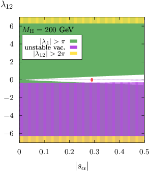
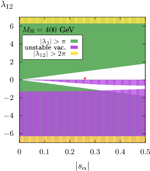
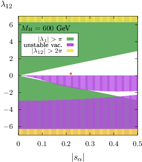
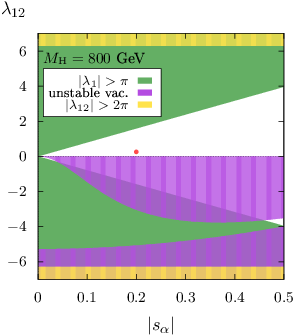
The allowed region is restricted to the white area, and it is possible to see how the condition on $\lambda_{1}$ presented in Eq. 6.6 plays an important role both for negative and positive $\lambda_{12}$ values. The vacuum stability condition (2.16) has an impact only on negative $\lambda_{12}$ values, ruling out a large part of space that is not excluded by perturbativity requirements. Green and yellow areas indicate regions where one can expect perturbativity problems, but should not be intended as sharp-cut regions. For the $M_{\text{H}}$ values considered here ( $200,400,600$ and $800\,\,\mathrm{GeV}$ ), the perturbativity of $\lambda_{12}$ does not affect the parameter space, but it becomes relevant for higher $M_{\text{H}}$ values. The perturbativity constraint on the coupling $\lambda_{2}$ is irrelevant in the considered regions.

6.3 Benchmark scenarios

For the numerical analysis we consider some of the benchmark scenarios proposed in Ref. [3], which were originally suggested in Ref. [37], adapting the input values to our needs. In Ref. [37], different values for the mass $M_{\text{H}}$ are considered (both lighter and heavier than $M_{\text{h}}$ ), and for each mass the mixing angle $\alpha$ is fixed to the maximal allowed value. Moreover, for mass values $M_{\text{H}}\geq 2M_{\text{h}}$ (i.e. when the $\text{H}\to\text{h}\text{h}$ decay is kinematically allowed), two values are proposed for $\tan\beta\equiv v_{2}/v_{1}$ , corresponding to the maximal and the minimal branching ratios for the $\text{H}\to\text{h}\text{h}$ decay.

Among these possibilities, we only consider scenarios in which $M_{\text{H}}>M_{\text{h}}$ (since the other possibility is phenomenologically disfavoured) and vary the heavy Higgs mass in the interval $200{-}800\,\,\mathrm{GeV}$ with $200\,\,\mathrm{GeV}$ steps. When two different $\tan\beta$ values are proposed, we consider the average. Since $\tan\beta$ enters in our calculation only at NLO and the two proposed values are always quite close, we expect negligible differences due to this choice.

We have to convert the numerical values of the input parameters given in Ref. [37] to our conventions. The SESM Higgs Lagrangian used here, as given in Eq. 2.2, is equivalent to the one given in Ref. [37] using the following substitutions,

\begin{split}\mu^{\text{ref}}&\to\sqrt{2}\mu_{1},\quad\lambda_{1}^{\text{ref}}\to\frac{\lambda_{2}}{4},\quad\lambda_{2}^{\text{ref}}\to 4\lambda_{1},\quad\lambda_{3}^{\text{ref}}\to 2\lambda_{12},\\ &\tan\beta^{\text{ref}}\to\frac{v_{2}}{v_{1}},\quad v^{\text{ref}}\to v_{2},\quad x^{\text{ref}}\to v_{1},\end{split}

(6.7)

where the label “ref” indicates the parameters used in Ref. [37], in which the numerical input is given in terms of $M_{\text{H}}$ , $\alpha$ , and $\tan\beta^{\text{ref}}$ . The heavy mass $M_{\text{H}}$ and the mixing angle $\alpha$ can be taken over directly. The scalar coupling $\lambda_{12}$ , which is a free parameter in our conventions, can be obtained from $\tan\beta^{\text{ref}}$ using the relations

\lambda_{12}=\frac{c_{\alpha}s_{\alpha}}{2v_{2}v_{1}}\left(M_{\text{H}}^{2}-M_{\text{h}}^{2}\right),\quad\tan\beta^{\text{ref}}=\frac{v_{2}}{v_{1}}.

(6.8)

We convert the benchmark points using Eqs. 6.7 and 6.8, rounding the $\lambda_{12}$ values to two decimal digits. The input values, in our convention, for the scenarios considered in our analysis are reported in Table 2 (together with the corresponding $\tan\beta^{\text{ref}}$ values).

\begin{array}[]{lccc}\hline\cr\hline\cr\text{Scenario}&M_{\text{H}}[\,\mathrm{GeV}]&\sin\alpha&\lambda_{12}\,(\tan\beta^{\text{ref}})\\ \hline\cr\text{BHM200${}^{\pm}$}&200&\pm 0.29&\pm 0.07\,(1.19)\\ \text{BHM400}&400&0.26&0.17\,(0.585)\\ \text{BHM600}&600&0.22&0.23\,(0.375)\\ \text{BHM800}&800&0.20&0.26\,(0.260)\\ \hline\cr\hline\cr\end{array}

Table 2: Input values for the SESM for a selection of benchmark scenarios for the SESM proposed in Refs. [3, 37], converted to the notation used in this work. In brackets, the

\tan\beta^{\text{ref}}

values used in Eq. 6.8 to compute the corresponding

\lambda_{12}

values are given.

For $M_{\text{H}}=200\,\,\mathrm{GeV}$ we discuss both signs of $s_{\alpha}$ with $|s_{\alpha}|=0.29$ ; for higher $M_{\text{H}}$ values we consider only positive $s_{\alpha}$ values, since the corresponding negative values are ruled out by the vacuum stability constraint. In the following we will make use of these scenarios in each of the renormalization schemes proposed in this paper.

7 Numerical analysis

In the following, we present the numerical results relevant for the decay $\text{h}\to 4f$ of the light Higgs boson of the SESM. Starting from benchmark scenario BHM200⁺, we show the effects of the conversion of the input variables between the two renormalization schemes presented in Sect. 4. Then we investigate the scale dependence of the parameters $\alpha$ and $\lambda_{12}$ , which are defined by ${\overline{\text{MS}}}$ renormalization conditions, by solving numerically the corresponding RGE. Afterwards, we present the results for the decay width $\Gamma_{\text{h}\to 4f}$ computed at different renormalization scales and show the deviations from the SM results as a function of the mixing angle. The same analysis is presented for benchmark scenario BHM600, while results for the scenarios BHM200^- and BHM400 are reported, respectively, in Appendices B and A. Finally, we show some differential distributions, comparing the results in the SM with the ones in the benchmark scenarios of Table 2.

7.1 BHM200⁺

7.1.1 Scheme conversion

When computing a physical observable at NLO accuracy, starting from a set of input parameters, it is crucial to realize that the input values correspond to a specific renormalization scheme adopted in the calculation. This becomes even more important when comparing NLO results for the same observable obtained using different renormalization schemes. In different schemes, the same numerical values for the input parameters represent different physical scenarios and, in order to have a sensible comparison of predictions for an observable in a given scenario, a proper conversion of the input parameters between the schemes is required.

In general, defining $N$ renormalized parameters $p_{i}$ in two renormalization schemes, denoted, respectively, by $p_{i}^{(1)}$ and $p_{i}^{(2)}$ , the relation between them is given by the solution of the following system of equations,

p_{i,0}=p_{i}^{(1)}+\delta p_{i}^{(1)}\bigl(p_{1}^{(1)},\dots,p_{N}^{(1)}\bigr)=p_{i}^{(2)}+\delta p_{i}^{(2)}\bigl(p_{1}^{(2)},\dots,p_{N}^{(2)}\bigr),

(7.1)

where the connection between the parameters in the two schemes is given by the bare parameters $p_{i,0}$ , which are independent of the renormalization scheme. In our particular case, converting the input values from the $\overline{\text{MS}}$ to the FJ scheme is quite simple, since, apart from the mixing angle $\alpha$ , all the other input parameters of the SESM have the same definition in the two schemes. Ignoring effects beyond NLO, the input parameters $p_{i}\neq\alpha$ are defined by identical renormalization conditions in the two schemes, i.e.

p_{i,0}=p_{i}^{\overline{\text{MS}}}+\delta p_{i}\bigl(\alpha^{\overline{\text{MS}}},\bigl\{p_{i}^{\overline{\text{MS}}}\bigr\}\bigr)=p_{i}^{\text{FJ}}+\delta p_{i}\bigl(\alpha^{\text{FJ}},\bigl\{p_{i}^{\text{FJ}}\bigr\}\bigr),

(7.2)

with identical counterterm functions $\delta p_{i}$ at NLO. This implies $p_{i}^{\overline{\text{MS}}}=p_{i}^{\text{FJ}}+{\cal O}\left(\alpha_{\text{em}}^{2}\right)$ , and we do not distinguish between $p_{i}^{\overline{\text{MS}}}$ and $p_{i}^{\text{FJ}}$ for parameters other than $\alpha$ . Equation 7.1 reduces to

\alpha_{0}=\alpha^{\overline{\text{MS}}}+\delta\alpha^{\overline{\text{MS}}}\bigl(\alpha^{\overline{\text{MS}}}\bigr)=\alpha^{\text{FJ}}+\delta\alpha^{\text{FJ}}\bigl(\alpha^{\text{FJ}}\bigr).

(7.3)

To solve the equation and find the relation between $\alpha^{\overline{\text{MS}}}$ and $\alpha^{\text{FJ}}$ , we adopt two strategies. In the first approach we linearize Eq. 7.3 and obtain

\alpha^{\text{FJ}}=\alpha^{\overline{\text{MS}}}+\delta\alpha^{\overline{\text{MS}}}\bigl(\alpha^{\overline{\text{MS}}}\bigr)-\delta\alpha^{\text{FJ}}\bigl(\alpha^{\overline{\text{MS}}}\bigr)+{\cal O}(\alpha_{\text{em}}^{2}).

(7.4)

Since our computations are performed at NLO, the ${\cal O}(\alpha_{\text{em}}^{2})$ term in Eq. 7.4 can be neglected. An analogous procedure can be applied to determine $\alpha^{\overline{\text{MS}}}$ when $\alpha^{\text{FJ}}$ is given as input. Using this method, converting an input value for the mixing angle from one scheme to the other and repeating the procedure to go back to the initial scheme, the final numerical result for $\alpha$ will change by contributions that are formally beyond NLO.

In the second approach, we solve Eq. 7.3 numerically, in order to keep the contributions of ${\cal O}(\alpha_{\text{em}}^{2})$ , which can become relevant for large counterterms or small tree-level values. Using this method, converting $\alpha$ to the other scheme and back, does not change the value of $\alpha$ . In the following results we use, as much as possible, the second method, i.e. we include the ${\cal O}(\alpha_{\text{em}}^{2})$ terms.

In Sect. 4.2 we have derived the counterterm $\delta\alpha$ in the two schemes, which differs by finite contributions,

\begin{split}\left.\delta\alpha^{\overline{\text{MS}}}\right|_{\text{finite}}&=0,\\ \left.\delta\alpha^{\text{FJ}}\right|_{\text{finite}}&=-\left.\Delta\alpha^{t}\left(T_{\text{h}},T_{\text{H}}\right)\right|_{\text{finite}}=\frac{e}{M_{\text{h}}^{2}-M_{\text{H}}^{2}}\left.\left(T_{\text{h}}\,\frac{C_{\text{h}\text{h}\text{H}}}{M_{\text{h}}^{2}}+T_{\text{H}}\,\frac{C_{\text{h}\text{H}\text{H}}}{M_{\text{H}}^{2}}\right)\right|_{\text{finite}},\end{split}

(7.5)

where the tadpoles $T_{\text{h}}$ , $T_{\text{H}}$ , and the coupling factors $C_{\text{h}\text{h}\text{H}}$ , $C_{\text{h}\text{H}\text{H}}$ in the last term depend on $\alpha^{\text{FJ}}$ . Using these expressions, it is straightforward to get the conversion from the FJ to the $\overline{\text{MS}}$ scheme,

\alpha^{\overline{\text{MS}}}=\alpha^{\text{FJ}}-\left.\Delta\alpha^{t}\left(T_{\text{h}},T_{\text{H}}\right)\right|_{\text{finite}},

(7.6)

while the conversion from $\overline{\text{MS}}$ to FJ requires a numerical solution of Eq. 7.6 for $\alpha^{\text{FJ}}$ , which appears also in the $\Delta\alpha^{t}$ term. In Fig. 9, we show the results for the conversion of the sine of the mixing angle, $s_{\alpha}$ , between the two schemes, both for the full solution of Eq. (7.3) and using the linearized solution (7.4).⁸⁸ 8 If Eq. (7.3) is used for the conversion, the corresponding curves in the two plots are related by a simple reflection about the diagonal $s_{\alpha}^{\overline{\text{MS}}}\equiv s_{\alpha}^{\text{FJ}}$ (apart from the different truncation of the curves in the non-perturbative region). The reflection symmetry is not there in the linearized version (7.4), but broken by effects beyond NLO. Note also that both versions coincide on the r.h.s., because $\delta\alpha^{\overline{\text{MS}}}$ does not contain finite contributions (UV divergent terms are canceled analytically). The curves on the right sides inside the plots are obtained fixing the mass $M_{\text{H}}$ of the heavy Higgs boson and the coupling $\lambda_{12}$ according to their values in the scenario BHM200⁺, reported in Table 2. On the left sides, similar curves show the conversion effects for negative $s_{\alpha}$ values. For consistency, we adjust the sign of $\lambda_{12}$ so that $\mathop{\mathrm{sgn}}\nolimits(s_{\alpha})=\mathop{\mathrm{sgn}}\nolimits(\lambda_{12})$ (for the input $s_{\alpha}$ ) and Eq. 2.12 is not violated. The renormalization scale is fixed to the mass of the light Higgs boson, $\mu_{\text{r}}=M_{\text{h}}$ ; the motivation for this choice will become clear in Sect. 7.1.3. The dark-gray shaded areas in the plots mark the values of $s_{\alpha}$ for which the perturbativity constraint (6.6) on $\lambda_{1}$ is violated; from the last line of Eq. (2.15) it is easily seen that $\lambda_{1}$ necessarily violates its perturbativity bound for $s_{\alpha}\to 0$ , since we keep $M_{\text{h}},M_{\text{H}},v_{2},\lambda_{12}$ fixed. The light-gray shaded areas denote regions where the sign of $s_{\alpha}$ is flipped by the conversion and becomes inconsistent with the sign of the considered $\lambda_{12}$ . The conversion effects in the perturbative regions are small: The red line is, in general, very close to the dashed diagonal line, which corresponds to the absence of any conversion effect (i.e. $s_{\alpha}^{\overline{\text{MS}}}=s_{\alpha}^{\text{FJ}}$ ), and the linearized solution reproduces the full conversion very well. Large effects (and deviations between full and linearized solutions) are only observed when approaching the non-perturbative regime, corresponding to small values of the mixing angle. In both plots of Fig. 9, a slight asymmetry can be observed between positive and negative $s_{\alpha}$ values, due to the different NLO contributions obtained by changing the sign of the input values for $s_{\alpha}$ and $\lambda_{12}$ .

7.1.2 Running of $s_{\alpha}$ and $\lambda_{12}$

Since we have defined the parameters $\alpha$ and $\lambda_{12}$ by ${\overline{\text{MS}}}$ renormalization conditions, they depend on an unphysical renormalization scale $\mu_{\text{r}}$ . The dependence on this scale is governed by the RGE

\frac{\partial}{\partial\ln\mu_{\text{r}}^{2}}\,\alpha\left(\mu_{\text{r}}^{2}\right)=\beta_{\alpha}\left(\mu_{\text{r}}^{2}\right),\qquad\frac{\partial}{\partial\ln\mu_{\text{r}}^{2}}\,\lambda_{12}\left(\mu_{\text{r}}^{2}\right)=\beta_{\lambda_{12}}\left(\mu_{\text{r}}^{2}\right),

(7.7)

where the $\beta_{\alpha}$ and $\beta_{\lambda_{12}}$ functions can be extracted from the expressions of the counterterms $\delta\alpha$ and $\delta\lambda_{12}$ , taking the coefficients of the UV divergence $\Delta_{\text{UV}}$ . These functions are different for the two considered renormalization schemes: For the $\overline{\text{MS}}$ scheme, the $\beta$ functions can be obtained considering the following derivatives with respect to the UV divergence,

\beta_{\alpha^{\overline{\text{MS}}}}=\frac{\partial}{\partial\Delta_{\text{UV}}}\delta\alpha^{\overline{\text{MS}}},\qquad\beta_{\lambda_{12}^{\overline{\text{MS}}}}=\frac{\partial}{\partial\Delta_{\text{UV}}}\delta\lambda_{12}^{\overline{\text{MS}}},

(7.8)

where the counterterm $\delta\alpha^{\overline{\text{MS}}}$ is given in Eqs. 4.18 and 4.19, and $\delta\lambda_{12}^{\overline{\text{MS}}}$ in Eqs. 4.22 and 4.23. For the FJ renormalization scheme, also the UV contributions due to the tadpoles must be taken into account, leading to the $\beta$ functions

\beta_{\alpha^{\text{FJ}}}=\beta_{\alpha^{\overline{\text{MS}}}}+\frac{\partial}{\partial\Delta_{\text{UV}}}\Delta\alpha^{t}\left(T_{\text{h}},T_{\text{H}}\right),\qquad\beta_{\lambda_{12}^{\text{FJ}}}=\beta_{\lambda_{12}^{\overline{\text{MS}}}},

(7.9)

where $\beta_{\lambda_{12}}$ is not changed due to the fact that $\delta\lambda_{12}$ is the same in the two schemes.

The RGE are coupled differential equations for which, in general, an analytical solution is not possible. We solve the equations numerically, using a Runge $-$ Kutta algorithm, obtaining the scale dependence for the sine of the mixing angle, $s_{\alpha}$ , and the coupling $\lambda_{12}$ , as shown in Fig. 10.

These results are obtained fixing the parameters $M_{\text{H}}$ , $\alpha$ , and $\lambda_{12}$ according to the values reported in Table 2 for benchmark scenario BHM200⁺ at the scale $\mu_{0}=M_{\text{h}}$ , and changing the scale $\mu_{\text{r}}$ in the range $50{-}350\,\,\mathrm{GeV}$ , using the $\beta$ functions for the two schemes. Since the purpose here is the assessment of the scale dependence of the ${\overline{\text{MS}}}$ parameters, no conversion between schemes is applied on the input values. In the two schemes, the scale dependence of $s_{\alpha}$ shows a completely different behaviour, while the running of $\lambda_{12}$ displays the same trend in the two schemes. As we will discuss below, the scale dependence of the mixing angle has a big impact on the scale variation of the decay width $\Gamma_{\text{h}\to 4f}$ .

7.1.3 Scale dependence of the inclusive decay width $\Gamma_{\text{h}\to 4f}$

In order to assign a sensible value to the renormalization scale $\mu_{\text{r}}$ , we study the impact of the scale choice on the results for $\Gamma_{\text{h}\to 4f}$ , the inclusive decay width of the light Higgs into four fermions. Taking the light Higgs mass as central renormalization scale, i.e. $\mu_{0}=M_{\text{h}}$ , we have computed the decay width at the scale $\mu_{\text{r}}$ in the range $50{-}350\,\,\mathrm{GeV}$ . The results are obtained fixing the input values for $M_{\text{H}}$ , $\alpha$ , and $\lambda_{12}$ at the central scale according to the scenario BHM200⁺ of Table 2 and shown in Fig. 11. In the figure, dashed lines correspond to the results for the LO decay width, and solid lines include NLO EW and QCD corrections. Magenta and blue lines represent, respectively, the results obtained in the $\overline{\text{MS}}$ and in the FJ renormalization schemes. On the left (right) panel the input parameters are defined in the $\overline{\text{MS}}$ (FJ) scheme and converted to the FJ ( $\overline{\text{MS}}$ ) scheme at the scale $\mu_{0}$ . The conversion is applied both for LO and NLO predictions. Note that the difference in the LO width observed at the central scale $\mu_{\text{r}}=\mu_{0}=M_{\text{h}}$ reflects the effect of the scheme conversion of $s_{\alpha}$ . Recalling that the expression of the LO matrix element is proportional to $c_{\alpha}$ , the behaviour of the LO results as a function of the renormalization scale is explained by the running of the mixing angle (shown in Fig. 10).

Comparing LO and NLO results, it is evident how the inclusion of loop contributions drastically reduces the scale dependence, as well as the scheme dependence: The solid lines are not only much flatter than the dashed lines, proving a reduced scale dependence, but solid curves of different colours are much closer to each other than the corresponding dashed curves. This is expected, since results obtained within different renormalization schemes should be equal up to higher-order contributions, provided that the input parameters are properly converted. The NLO predictions, in particular, perfectly coincide at the central scale $\mu_{\text{r}}=\mu_{0}=M_{\text{h}}$ . Quantifying the scale dependence by the change in $\Gamma_{\text{h}\to 4f}$ obtained by varying the scale $\mu_{\text{r}}$ by factors of two up and down ( $\mu_{\text{r}}=2\mu_{0}$ and $\mu_{\text{r}}=\mu_{0}/2$ ), we observe a reduction from $\sim 3{-}4\%$ at LO to $\mathrel{\raisebox{-3.00003pt}{$\stackrel{{\scriptstyle\displaystyle<}}{{\sim}}$}}0.5\%$ at NLO. The scheme dependence, defined by the relative difference between the results in the ${\overline{\text{MS}}}$ and FJ schemes at the central scale, on the other hand, reduces from $\sim 1\%$ at LO to $\mathrel{\raisebox{-3.00003pt}{$\stackrel{{\scriptstyle\displaystyle<}}{{\sim}}$}}0.1\%$ at NLO.

As discussed in Refs. [43, 56] for NLO predictions of $\Gamma_{\text{h}\to 4f}$ in the THDM, when the computation involves multiple mass scales in the loops, it is not clear a priori that the central scale $\mu_{0}=M_{\text{h}}$ is an appropriate choice. In principle, this applies also to the SESM, where the heavy Higgs boson appears in loop diagrams. However, it is evident from Fig. 11 how the scale dependence is minimized for values around the light Higgs mass. On the other hand, using the alternative scale $\mu_{0}=(M_{\text{h}}+M_{\text{H}})/2$ analogous to the scale choice advocated in Ref. [43] for the THDM, would not make a big difference for the scenario BHM200⁺, due to the relatively small value for the heavy Higgs mass, fixed at $M_{\text{H}}=200\,\,\mathrm{GeV}$ . As discussed later in the section, repeating the same analysis on the scale variation with higher $M_{\text{H}}$ values, we will see how the scale $\mu_{0}=M_{\text{h}}$ is better than the alternative scale given by the arithmetic mean of the Higgs-boson masses. Note that finding optimal scales, to some extent, is empirical, i.e. the scale dependence should be investigated whenever qualitatively new scenarios are considered.

7.1.4 Mixing-angle dependence of the inclusive decay width $\Gamma_{\text{h}\to 4f}$

Among the free parameters of the SESM, the mixing angle $\alpha$ plays the central role in the computation of the decay width $\Gamma_{\text{h}\to 4f}$ . Its value affects already the LO result, while the heavy Higgs mass $M_{\text{H}}$ and the coupling $\lambda_{12}$ enter only the NLO decay amplitudes. For this reason, we compute the decay width varying $s_{\alpha}$ in the range $0.01{-}0.3$ , keeping $M_{\text{H}}$ and $\lambda_{12}$ fixed according to the values for benchmark scenario BHM200⁺.⁹⁹ 9 Within this analysis, we exclude the value $s_{\alpha}=0$ , since in this case Eq. 2.15 would imply $v_{1}=0$ , for a given non-vanishing $\lambda_{12}$ . We consider both $\overline{\text{MS}}$ and FJ as input schemes and compute the decay width in the two schemes, using the renormalization scale $\mu_{\text{r}}=M_{\text{h}}$ . The results for $\Gamma_{\text{h}\to 4f}$ are reported in Fig. 12, where we also show the SM value of the decay width identifying h with the SM Higgs boson.

Dashed and solid lines denote, respectively, the LO and the NLO results, where the latter include both EW and QCD corrections. The dashed vertical line indicates the minimal $s_{\alpha}$ value for which the perturbativity conditions of Eq. 6.6 are satisfied. Differences between the LO results in the two schemes (within the same plot) are due to the scheme conversion, which is done at NLO. Comparing the LO results, it is possible to observe the suppression with respect to the SM given by the $c_{\alpha}^{2}$ factor, coming from the square of Eq. 5.5. The proportionality to $c_{\alpha}^{2}=1-s_{\alpha}^{2}$ is exact if no conversion of the input is done, i.e. on the left (right) side for the LO $\overline{\text{MS}}$ (FJ) curve. The NLO contributions modify the $s_{\alpha}$ dependence, so that for $s_{\alpha}\sim 0.08$ the NLO decay width is the same as in the SM, and in general the difference between SESM and SM are smaller for the NLO decay width. Note also the reduction of the scheme dependence at NLO, visible by the fact that $\overline{\text{MS}}$ and FJ curves practically lie on top of each other.

In Fig. 13 we show the relative corrections $\delta_{\text{NLO}}$ to the inclusive $\text{h}\to 4f$ decay width, defined by

\delta_{\text{NLO}}=\frac{\Gamma_{\text{NLO}}-\Gamma_{\text{LO}}}{\Gamma_{\text{LO}}}=\delta_{\text{EW}}+\delta_{\text{QCD}},

(7.10)

where the NLO result includes both EW ( $\delta_{\text{EW}}$ ) and QCD corrections ( $\delta_{\text{QCD}}$ ). The relative QCD corrections do not depend on the mixing angle and are equal to the SM case, providing an offset of about $5\%$ . The relative corrections in the SESM are, for the scenario considered here, bigger than the relative corrections in the SM case, somewhat compensating the LO suppression factor $c_{\alpha}^{2}$ mentioned above. For $s_{\alpha}=0.29$ , as defined for the scenario BHM200⁺, the relative corrections are $9.6\%$ in the FJ scheme and $8.6\%$ in the $\overline{\text{MS}}$ scheme. Figure 13 illustrates that in the two schemes contributions (related to the tadpole terms) are shared differently between LO and NLO parts.

Recall that we have seen in Fig. 12 how the NLO decay widths are in good agreement in the two renormalization schemes, independent of the $s_{\alpha}$ value.

In Fig. 14 we compare the SESM result with the SM prediction, defining the relative deviation by

\Delta_{\text{SM}}=\frac{\Gamma_{\text{SESM}}-\Gamma_{\text{SM}}}{\Gamma_{\text{SM}}}.

(7.11)

Again, it is possible to see how the negative deviations induced by the $c_{\alpha}^{2}$ factor are somewhat reduced at NLO due to the positive loop contributions, which in the SESM are bigger than in the SM. For $s_{\alpha}=0.29$ , corresponding to the scenario BHM200⁺, the deviations from the SM are $\Delta_{\text{SM}}\sim 7{-}8\%$ . The difference between the results shown in the two panels, which correspond to $s_{\alpha}$ values in the two different renormalization schemes, is due to the fact that, changing the input scheme, the same numerical values correspond to different physical scenarios.

7.1.5 Decay widths for individual four-fermion final states

In Table 3 we compile our results on the widths for the decays $\text{h}\to 4f$ into the various different final states for benchmark scenario BHM200⁺, computed in the FJ scheme.

\begin{array}[]{cccccc}\hline\cr\hline\cr\text{Final state}&\Gamma^{\text{NLO}}_{\text{h}\to 4f}&\delta_{\text{EW}}[\%]&\delta_{\text{QCD}}[\%]&\Delta_{\text{SM}}^{\text{NLO}}[\%]&\Delta_{\text{SM}}^{\text{LO}}[\%]\\ \hline\cr\text{inclusive}\,\text{h}\to 4f&0.92106(6)&4.64(0)&4.97(0)&-6.82(1)&-8.41(1)\\ \text{Z}\text{Z}&0.101320(5)&2.35(0)&4.89(0)&-6.78(1)&-8.41(0)\\ \text{W}\text{W}&0.82459(8)&4.92(0)&5.01(1)&-6.82(1)&-8.41(1)\\ \text{W}\text{W}/\text{Z}\text{Z}\text{int.}&-0.00485(5)&3.3(2)&11.4(8)&-7(1)&-8.4(6)\\ \nu_{\text{e}}\text{e}^{+}\mu^{-}\bar{\nu}_{\mu}&0.009719(1)&4.95(0)&0.00&-6.75(1)&-8.41(1)\\ \nu_{\text{e}}\text{e}^{+}\text{u}\bar{\text{d}}&0.030198(4)&4.94(0)&3.76(1)&-6.80(2)&-8.41(1)\\ \text{u}\bar{\text{d}}\text{s}\bar{\text{c}}&0.09369(2)&4.89(0)&7.52(1)&-6.86(2)&-8.41(1)\\ \nu_{\text{e}}\text{e}^{+}\text{e}^{-}\bar{\nu}_{\text{e}}&0.009716(1)&5.05(0)&0.00&-6.75(1)&-8.41(1)\\ \text{u}\bar{\text{d}}\text{d}\bar{\text{u}}&0.09562(2)&4.77(0)&7.36(1)&-6.86(2)&-8.41(1)\\ \nu_{\text{e}}\bar{\nu}_{\text{e}}\nu_{\mu}\bar{\nu}_{\mu}&0.000906(0)&5.02(0)&0.00&-6.75(1)&-8.41(1)\\ \text{e}^{-}\text{e}^{+}\mu^{-}\mu^{+}&0.000228(0)&3.31(1)&0.00&-6.72(1)&-8.41(1)\\ \nu_{\text{e}}\bar{\nu}_{\text{e}}\mu^{-}\mu^{+}&0.000456(0)&4.47(1)&0.00&-6.74(2)&-8.41(1)\\ \nu_{\text{e}}\bar{\nu}_{\text{e}}\nu_{\text{e}}\bar{\nu}_{\text{e}}&0.000543(0)&4.91(0)&0.00&-6.75(1)&-8.41(1)\\ \text{e}^{-}\text{e}^{+}\text{e}^{-}\text{e}^{+}&0.000126(0)&3.14(1)&0.00&-6.72(1)&-8.41(1)\\ \nu_{\text{e}}\bar{\nu}_{\text{e}}\text{u}\bar{\text{u}}&0.001603(0)&2.60(1)&3.76(1)&-6.77(1)&-8.41(1)\\ \nu_{\text{e}}\bar{\nu}_{\text{e}}\text{d}\bar{\text{d}}&0.002078(0)&3.70(0)&3.76(1)&-6.79(2)&-8.41(1)\\ \text{e}^{-}\text{e}^{+}\text{u}\bar{\text{u}}&0.000807(0)&2.12(1)&3.75(1)&-6.76(1)&-8.41(1)\\ \text{e}^{-}\text{e}^{+}\text{d}\bar{\text{d}}&0.001039(0)&2.48(1)&3.76(1)&-6.77(2)&-8.41(1)\\ \text{u}\bar{\text{u}}\text{c}\bar{\text{c}}&0.002836(0)&0.21(1)&7.51(1)&-6.79(2)&-8.41(1)\\ \text{d}\bar{\text{d}}\text{d}\bar{\text{d}}&0.002444(1)&1.62(0)&4.53(2)&-6.76(3)&-8.41(1)\\ \text{d}\bar{\text{d}}\text{s}\bar{\text{s}}&0.004729(1)&1.65(0)&7.51(1)&-6.81(2)&-8.41(1)\\ \text{u}\bar{\text{u}}\text{s}\bar{\text{s}}&0.003676(1)&1.34(1)&7.51(1)&-6.80(2)&-8.41(1)\\ \text{u}\bar{\text{u}}\text{u}\bar{\text{u}}&0.001441(0)&0.09(1)&4.22(2)&-6.73(3)&-8.41(1)\\ \hline\cr\hline\cr\end{array}

Table 3: Partial widths for scenario BHM200⁺ in the FJ renormalization scheme. The integration errors are given in parentheses.

The contributions $\Gamma_{\text{h}\to\text{W}\text{W}\to 4f}$ , $\Gamma_{\text{h}\to\text{Z}\text{Z}\to 4f}$ , and $\Gamma_{\text{W}\text{W}/\text{Z}\text{Z}-\text{int}}$ are calculated according to Eq. 5.4, and the total decay width $\Gamma_{\text{h}\to 4f}$ using Eq. 5.1. In Table 3, we also show the relative EW and QCD corrections, $\delta_{\text{EW}}$ and $\delta_{\text{QCD}}$ , and in the last two columns the deviation $\Delta_{\text{SM}}$ from the SM both at LO and NLO. For all the quantities, we report the integration uncertainty in parentheses. To determine the errors of the decay widths to WW, ZZ, $\text{W}\text{W}/\text{Z}\text{Z}$ interference and of the total width $\Gamma_{\text{h}\to 4f}$ , we apply the standard error propagation to Eqs. 5.4 and 5.1, making use of the integration uncertainties for each single final state.

The main contribution to the total $\text{h}\to 4f$ decay width originates from the charge-current final states, while the neutral-current processes have a smaller impact, and the $\text{W}\text{W}/\text{Z}\text{Z}$ interference gives a very small negative contribution. The EW corrections to the WW contributions are about $5\%$ , and lead to a similar value for the inclusive decay $\text{h}\to 4f$ . The EW corrections to neutral-current final states range from $0$ to $5\%$ , depending on the flavour of the final-state fermions. The QCD corrections are mostly due to the corrections to the decays $\text{W}/\text{Z}\to\text{q}\bar{\text{q}}$ , and amount to $\alpha_{\text{s}}/\pi$ for each quark pair in the final state. Exceptions are the final states $\text{u}\bar{\text{u}}\text{u}\bar{\text{u}}$ and $\text{d}\bar{\text{d}}\text{d}\bar{\text{d}}$ , where interference contributions from two different topologies of the ZZ channel occur, and the QCD corrections to these final states are only about $4\%$ . The SM deviation, at LO, comes from the $c_{\alpha}$ rescaling factor of the $hVV$ coupling with respect to the SM coupling, and is equal to $c_{\alpha}^{2}-1=-0.0841$ in the considered scenario. As already observed in the previous section, at NLO the deviations from the SM are about $1.5\%$ smaller.

We have computed the same quantities as in Table 3 in the $\overline{\text{MS}}$ scheme, observing somewhat smaller values for the EW corrections, since in the two schemes contributions are shared differently between the LO and the NLO (as observed also in Fig. 13). Moreover, using the same numerical input in the $\overline{\text{MS}}$ input scheme leads to NLO deviations from the SM about $1\%$ higher, since the same numerical input corresponds to a slightly different physical scenario. In total, the $\overline{\text{MS}}$ results follow the same qualitative pattern as in the FJ scheme, and are not reported here.

7.2 BHM600

7.2.1 Scheme conversion

In Fig. 15 we show the conversion of the input value for $s_{\alpha}$ from the $\overline{\text{MS}}$ to the FJ scheme (left panel) and vice versa (right panel).

The values of $M_{\text{H}}$ and $|\lambda_{12}|$ are given in the scenario BHM600 as stated in Table 2. For consistency, for negative $s_{\alpha}$ input values we consider a negative Higgs self-coupling $\lambda_{12}$ . The renormalization scale $\mu_{\text{r}}$ is again chosen to be equal to the light Higgs mass $M_{\text{h}}$ . For the considered values of the input parameters, the perturbativity constraint on $\lambda_{1}$ of Eq. 6.6 is violated for $|s_{\alpha}|\lesssim 0.04$ . The dark-gray shaded area corresponds to the region where the perturbativity condition breaks down. The light-gray areas denote regions where the vacuum stability condition (2.16) is violated and where the sign of $s_{\alpha}$ becomes different from the sign of $\lambda_{12}$ by effect of the conversion. As discussed in Sect. 7.1.1, the conversion from the FJ to the $\overline{\text{MS}}$ scheme can be computed straightforwardly from the matching condition (7.3), while to compute the inverse conversion the matching condition has to be solved numerically. Alternatively, the linear approximation (7.4) may be used. In the left panel of Fig. 15 we use the linear approximation (shown in blue) in the non-perturbative region, where the numerical inversion does not provide a solution. The red lines correspond to the results obtained from the numerical solution of the non-linearized matching equation (7.3). The conversion effects are small for $|s_{\alpha}|\sim 0.3$ and become large for small angles. The conversion has an important impact in the vicinity of the non-perturbative region, where loop effects exceed the LO contributions. Asymmetries of the plots are due to the different sign used for $\lambda_{12}$ , so that $\mathop{\mathrm{sgn}}\nolimits(s_{\alpha})=\mathop{\mathrm{sgn}}\nolimits(\lambda_{12})$ .

7.2.2 Running of $s_{\alpha}$ and $\lambda_{12}$

The solution of the RGE for the ${\overline{\text{MS}}}$ parameters $s_{\alpha}$ and $\lambda_{12}$ is shown in Fig. 16 for scenario BHM600.

The solutions are again obtained numerically by a Runge $-$ Kutta algorithm. The values for the BSM parameters $s_{\alpha}$ , $M_{\text{H}}$ , and $\lambda_{12}$ are fixed according to scenario BHM600 at the scale $\mu_{0}=M_{\text{h}}$ and evolved to the renormalization scale $\mu_{\text{r}}$ in the range $\mu_{\text{r}}=50{-}350\,\,\mathrm{GeV}$ . We report the results both for the $\overline{\text{MS}}$ and the FJ schemes, where we can observe a different behaviour in the running of $s_{\alpha}$ : The sine of the mixing angle increases with the scale in the FJ scheme, while it slowly decreases in the $\overline{\text{MS}}$ scheme. The running of the coupling $\lambda_{12}$ , in the considered range, is almost identical in the two schemes. Compared to the scenario BHM200⁺, the running of $s_{\alpha}$ in the $\overline{\text{MS}}$ scheme is strongly reduced.

7.2.3 Scale dependence of the inclusive decay width $\Gamma_{\text{h}\to 4f}$

In Fig. 17 we present the results for the inclusive decay width $\Gamma_{\text{h}\to 4f}$ for scenario BHM600 at scales $\mu_{\text{r}}$ in the range $50{-}350\,\,\mathrm{GeV}$ .

The results obtained using the $\overline{\text{MS}}$ (magenta) and the FJ (blue) input schemes are reported, respectively, on the left and the right panels of the figure. Dashed lines correspond to the LO results (with NLO conversion of the input parameters), solid lines include NLO EW+QCD corrections. Similar to the observations made for scenario BHM200⁺ above, the NLO results show a much milder scale dependence compared to the LO results, and the differences between the two schemes are strongly reduced. We can see that the scale choice $\mu_{\text{r}}=M_{\text{h}}$ seems more suitable than the alternative scale $\mu_{\text{r}}=(M_{\text{h}}+M_{\text{H}})/2\sim 360\,\,\mathrm{GeV}$ , where the dependence on the renormalization scale is somewhat stronger. Quantitatively, the scale dependence (again defined by scale variations of factors $2$ and $1/2$ ) reduces from $\sim 1{-}2\%$ at LO to $\sim 0.3\%$ at NLO in the FJ scheme, while the scale dependence in the ${\overline{\text{MS}}}$ scheme is at the $0.1\%$ level both at LO and NLO due to the suppression of the running of $\alpha$ in the BHM600 scenario. The scheme dependence at the central scale reduces from $\sim 0.8\%$ at LO to $\sim 0.1\%$ at NLO.

7.2.4 Mixing-angle dependence of the inclusive decay width $\Gamma_{\text{h}\to 4f}$

In Figs. 18, 19 and 20 we present, respectively, the decay width $\Gamma_{\text{h}\to 4f}$ , the relative corrections to the decay width, and the deviations with respect to the SM result as a function of the parameter $s_{\alpha}$ using our default scale choice $\mu_{\text{r}}=\mu_{0}=M_{\text{h}}$ .

The heavy Higgs mass and the coupling $\lambda_{12}$ are fixed according to scenario BHM600, as defined in Table 2. In all the figures, dashed lines correspond to LO results and solid lines to NLO results, including both EW and QCD corrections. We consider values $|s_{\alpha}|<0.3$ and mark with a dashed vertical line the minimal $s_{\alpha}$ value for which the perturbativity constraints of Eq. 6.6 are fulfilled. The results reported in the left (right) panel are obtained with input parameters defined in $\overline{\text{MS}}$ (FJ) scheme with a proper parameter conversion at NLO applied if the input is not directly given in the scheme used in the calculation.

In the LO results of Fig. 18, the $c_{\alpha}^{2}$ dependence of the decay width in the SESM is manifest, where the proportionality to $c_{\alpha}^{2}$ is exact if no scheme conversion is involved. For small mixing angles, where $c_{\alpha}\to 1$ , the deviations from the SM are due to the conversion effects. As observed in the other scenarios, the inclusion of NLO corrections slightly compensates the $c_{\alpha}^{2}$ suppression for small $s_{\alpha}$ values. Moreover, we observe that the two schemes are in much better agreement after the inclusion of NLO corrections, i.e. the inclusion of NLO corrections reduces the renormalization scheme dependence drastically.

The relative NLO corrections, as defined in Eq. 7.10, are shown in Fig. 19 including both EW and QCD contributions (the latter are independent of $s_{\alpha}$ and about $5\%$ ). In the considered $s_{\alpha}$ range the relative corrections amount to $7{-}9\%$ (slightly depending on the input scheme used) and the difference with the SM relative corrections $|\delta^{\text{SESM}}-\delta^{\text{SM}}|$ does not exceed the $1\%$ level in the considered region.

In Fig. 20 we illustrate the deviations from the SM, defined by Eq. 7.11. It is possible to see how the NLO results converge nicely in the two schemes. Note that the large scheme-dependence due to missing higher-orders for small $s_{\alpha}$ values occurs only in the non-perturbative regime, where calculations generally become unreliable. The proposed $s_{\alpha}$ values for the scenario BHM600 is $0.22$ , yielding a deviation from the SM of about $-5\%$ .

7.2.5 Decay widths for individual four-fermion final states

In Table 4 we compile the results for the $\text{h}\to 4f$ decay widths for each final state listed in Table 1, together with the widths for the decays into two vector bosons and the inclusive decay width $\Gamma_{\text{h}\to 4f}$ .

\begin{array}[]{cccccc}\hline\cr\hline\cr\text{Final state}&\Gamma^{\text{NLO}}_{\text{h}\to 4f}&\delta_{\text{EW}}[\%]&\delta_{\text{QCD}}[\%]&\Delta_{\text{SM}}^{\text{NLO}}[\%]&\Delta_{\text{SM}}^{\text{LO}}[\%]\\ \hline\cr\text{inclusive}\,\text{h}\to 4f&0.93761(6)&2.42(0)&4.97(0)&-5.14(1)&-4.84(1)\\ \text{Z}\text{Z}&0.103098(5)&0.13(0)&4.89(0)&-5.15(1)&-4.84(0)\\ \text{W}\text{W}&0.83945(8)&2.71(0)&5.01(1)&-5.14(1)&-4.84(1)\\ \text{W}\text{W}/\text{Z}\text{Z}\text{int.}&-0.00494(5)&1.1(2)&11.4(8)&-5(1)&-4.8(7)\\ \nu_{\text{e}}\text{e}^{+}\mu^{-}\bar{\nu}_{\mu}&0.009884(1)&2.73(0)&0.00&-5.16(1)&-4.84(1)\\ \nu_{\text{e}}\text{e}^{+}\text{u}\bar{\text{d}}&0.030736(4)&2.73(0)&3.76(1)&-5.15(2)&-4.84(1)\\ \text{u}\bar{\text{d}}\text{s}\bar{\text{c}}&0.09542(2)&2.68(0)&7.52(1)&-5.14(2)&-4.84(1)\\ \nu_{\text{e}}\text{e}^{+}\text{e}^{-}\bar{\nu}_{\text{e}}&0.009882(1)&2.83(0)&0.00&-5.16(1)&-4.84(1)\\ \text{u}\bar{\text{d}}\text{d}\bar{\text{u}}&0.09739(2)&2.56(0)&7.36(1)&-5.14(2)&-4.84(1)\\ \nu_{\text{e}}\bar{\nu}_{\text{e}}\nu_{\mu}\bar{\nu}_{\mu}&0.000921(0)&2.80(0)&0.00&-5.16(1)&-4.84(1)\\ \text{e}^{-}\text{e}^{+}\mu^{-}\mu^{+}&0.000232(0)&1.10(1)&0.00&-5.16(1)&-4.84(1)\\ \nu_{\text{e}}\bar{\nu}_{\text{e}}\mu^{-}\mu^{+}&0.000464(0)&2.25(1)&0.00&-5.16(2)&-4.84(1)\\ \nu_{\text{e}}\bar{\nu}_{\text{e}}\nu_{\text{e}}\bar{\nu}_{\text{e}}&0.000552(0)&2.69(0)&0.00&-5.16(1)&-4.84(1)\\ \text{e}^{-}\text{e}^{+}\text{e}^{-}\text{e}^{+}&0.000128(0)&0.93(1)&0.00&-5.16(1)&-4.84(1)\\ \nu_{\text{e}}\bar{\nu}_{\text{e}}\text{u}\bar{\text{u}}&0.001631(0)&0.39(1)&3.76(1)&-5.15(1)&-4.84(1)\\ \nu_{\text{e}}\bar{\nu}_{\text{e}}\text{d}\bar{\text{d}}&0.002114(0)&1.48(0)&3.76(1)&-5.15(2)&-4.84(1)\\ \text{e}^{-}\text{e}^{+}\text{u}\bar{\text{u}}&0.000821(0)&-0.09(1)&3.75(1)&-5.15(2)&-4.84(1)\\ \text{e}^{-}\text{e}^{+}\text{d}\bar{\text{d}}&0.001057(0)&0.27(1)&3.76(1)&-5.15(2)&-4.84(1)\\ \text{u}\bar{\text{u}}\text{c}\bar{\text{c}}&0.002886(0)&-2.00(1)&7.51(1)&-5.14(2)&-4.84(1)\\ \text{d}\bar{\text{d}}\text{d}\bar{\text{d}}&0.002486(1)&-0.59(0)&4.53(2)&-5.15(3)&-4.84(1)\\ \text{d}\bar{\text{d}}\text{s}\bar{\text{s}}&0.004814(1)&-0.56(0)&7.51(1)&-5.14(2)&-4.84(1)\\ \text{u}\bar{\text{u}}\text{s}\bar{\text{s}}&0.003742(1)&-0.87(1)&7.51(1)&-5.14(2)&-4.84(1)\\ \text{u}\bar{\text{u}}\text{u}\bar{\text{u}}&0.001465(0)&-2.11(1)&4.22(2)&-5.14(3)&-4.84(1)\\ \hline\cr\hline\cr\end{array}

Table 4: Partial widths for scenario BHM600 in the FJ renormalization scheme. The integration errors are given in parentheses.

For each decay channel, we report the NLO result, the EW and QCD relative corrections, and the deviations from the SM result. The latter are reported both for LO and NLO. The qualitative picture is basically the same as for the scenarios BHM200⁺, with slightly different values for the EW corrections, which are between $-2\%$ and $3\%$ , i.e. a bit smaller than in the other cases with smaller $M_{\text{H}}$ . The deviation from the SM is about $-5\%$ , in the FJ scheme, at LO and NLO. Using the $\overline{\text{MS}}$ input scheme, the deviations $\Delta_{\text{SM}}^{\text{NLO}}$ are only slightly different, around $-4.5\%$ , and display a similar pattern.

7.3 Differential distributions

Footprints of potential BSM physics often can be found by looking into the shapes of differential distributions, even if integrated results do not deviate from the SM predictions significantly. In the following, we discuss some of the distributions produced with Prophecy4f for the SESM, reporting results both for charged- and neutral-current final states. The generator provides invariant-mass and angular distributions for leptonic and semi-leptonic final states, while distributions for fully hadronic final states are not interesting, since they are not experimentally accessible. A detailed survey of distributions in the SM can be found in Refs. [53, 52, 54] for fully leptonic final states and in Ref. [51] for the semi-leptonic case. There, the treatment of the final-state radiation and the photon recombination for nearly collinear fermion $-$ photon pairs are also discussed in detail. In the SESM, relative corrections induced by final-state radiation are identical to the SM case and thus not discussed in greater detail here.

7.3.1 Leptonic final states

We consider the fully leptonic final states ${\mu^{-}}{\mu^{+}}{\text{e}^{-}}{\text{e}^{+}}$ and $\nu_{\mu}{\mu^{+}}{\text{e}^{-}}\nu_{\text{e}}$ , which involve, respectively, intermediate (off-shell) WW and ZZ states. The distributions discussed in the following have been computed in the FJ renormalization scheme, the results obtained in the $\overline{\text{MS}}$ scheme show the same features and are not reported here. All the distributions are generated using the renormalization scale $\mu_{\text{r}}=M_{\text{h}}$ .

For the neutral-current final state ${\mu^{-}}{\mu^{+}}{\text{e}^{-}}{\text{e}^{+}}$ , the left panel of Fig. 21 shows the NLO distribution for the invariant mass of the muon pair around the Z-boson resonance, both for the SM and for the considered SESM scenarios.

In general, the invariant mass of a fermionic pair is defined by

M_{f_{a}\bar{f}_{b}}=\left(k_{a}+k_{b}\right)^{2},

(7.12)

where $k_{a}$ and $k_{b}$ are the four-momenta of the fermion $f_{a}$ and the anti-fermion $\bar{f}_{b}$ and, in case of photon recombination, the photon momentum is added to the momentum of the fermion or anti-fermion. The distributions obtained for the SESM display the Z-boson resonance peak and the “radiative tail” observed in the standard case: The real-emission contributions lead to positive corrections for invariant masses below the Z-boson peak. This is explained by the fact that outgoing leptons lose momentum when radiating a photon, so that these events are shifted towards lower masses. This can be seen in the lower panel of the plot, where the relative NLO corrections $\delta_{\text{NLO}}$ are shown bin-by-bin. The shapes of the distributions in the SESM are the same as in the SM, and the only difference is given by an offset, which depends on the SESM scenario. The difference between the NLO distribution in the SM and in the SESM equals, for each considered scenario, the quantity $\Delta_{\text{SM}}^{\text{NLO}}$ obtained for the corresponding integrated result (see Tables 3 and 4 for BHM200⁺ and BHM600). We observe this pattern in all the generated distributions. The right panel of Fig. 21 shows, for the same final state, the differential decay width with respect to the angle $\phi$ , which is defined as the angle between the decay planes of the two intermediate Z bosons in the Higgs rest frame,

\cos\phi=\frac{\left(\left(\mathbf{k}_{\mu^{+}}+\mathbf{k}_{\mu^{-}}\right)\times\mathbf{k}_{\mu^{+}}\right)\cdot((\mathbf{k}_{\mu^{+}}+\mathbf{k}_{\mu^{-}})\times\mathbf{k}_{\text{e}^{+}})}{|(\mathbf{k}_{\mu^{+}}+\mathbf{k}_{\mu^{-}})\times\mathbf{k}_{\mu^{+}}|\,|(\mathbf{k}_{\mu^{+}}+\mathbf{k}_{\mu^{-}})\times\mathbf{k}_{\text{e}^{+}}|},

(7.13)

with the sign convention

\text{sgn}(\sin\phi)=\text{sgn}\left\{\left(\mathbf{k}_{\mu^{+}}+\mathbf{k}_{\mu^{-}}\right)\cdot\left[\left(\left(\mathbf{k}_{\mu^{+}}+\mathbf{k}_{\mu^{-}}\right)\times\mathbf{k}_{\mu^{+}}\right)\times\left(\left(\mathbf{k}_{\mu^{+}}+\mathbf{k}_{\mu^{-}}\right)\times\mathbf{k}_{\text{e}^{+}}\right)\right]\right\}.

(7.14)

The distribution resembles a $\cos(2\phi)$ oscillation with some constant offset and can be used to determine the parity of the Higgs boson and to set bounds on BSM couplings to EW gauge bosons of the decaying scalar (see Refs. [83, 84, 85, 86, 87, 88, 89, 90]). As observed for the invariant-mass distributions, the shape of the distributions in the SESM scenarios is the same as in the SM, and the NLO relative corrections differ just by a constant offset which is equivalent to $\Delta_{\text{SM}}^{\text{NLO}}$ observed for the integrated widths.

Figure 22 shows differential distributions for the charged-current final state $\nu_{\mu}{\mu^{+}}{\text{e}^{-}}\nu_{\text{e}}$ for the SM and the SESM.

The invariant-mass distribution for $M_{\nu_{\mu}\mu}$ , shown in the left panel of the figure, is not experimentally accessible, but is interesting from the theoretical point of view. The distribution shows the W-boson resonance and the radiative tail already described for the ${\mu^{-}}{\mu^{+}}{\text{e}^{-}}{\text{e}^{+}}$ final state, with an enhancement below the W-boson peak driven by the real photon emission. The SESM does not induce any additional distortion on top of the SM shape. The corrections and the differences between the SM and the SESM scenarios match always the values obtained for the integrated results. The right panel of the figure shows the distribution for the angle between the transverse momenta of the muon and the electron, in the Higgs rest frame, defined by

\cos\phi_{\mu\text{e},\text{T}}=\frac{\mathbf{k}_{\mu,\text{T}}\cdot\mathbf{k}_{\text{e},\text{T}}}{|\mathbf{k}_{\mu,\text{T}}|\,|\mathbf{k}_{\text{e},\text{T}}|},\qquad\text{sgn}(\sin\phi_{\text{T}})=\text{sgn}\{\mathbf{e}_{z}\cdot(\mathbf{k}_{\mu,\text{T}}\times\mathbf{k}_{\text{e},\text{T}})\},

(7.15)

where $\mathbf{k}_{i,\text{T}}$ are the projections of the lepton momenta onto the plane orthogonal to the unit vector $\mathbf{e}_{z}$ , which denotes the beam direction of the Higgs production process. The distributions, in the SESM, have the same shape as in the SM, and the relative NLO corrections, reported in the lower panel, are the same as in the SM up to constant offsets. As observed in the other cases, the differences between the SM result and the ones in the various SESM scenarios can be quantified by the corresponding $\Delta_{\text{SM}}^{\text{NLO}}$ obtained for the integrated decay width.

7.3.2 Semi-leptonic final states

In the following, we present differential distributions obtained for the semi-leptonic final states $\text{d}\bar{\text{d}}{\text{e}^{-}}{\text{e}^{+}}$ and $\nu_{\text{e}}{\text{e}^{+}}\text{d}\bar{\text{u}}$ , computed in the FJ renormalization scheme. In the ${\overline{\text{MS}}}$ renormalization scheme, the distributions show similar features and are not reported here. The renormalization scale used to generate the distributions is again $\mu_{\text{r}}=M_{\text{h}}$ .

In Fig. 23 we depict differential distributions for the neutral-current final state $\text{d}\bar{\text{d}}{\text{e}^{-}}{\text{e}^{+}}$ , including both EW and QCD corrections.

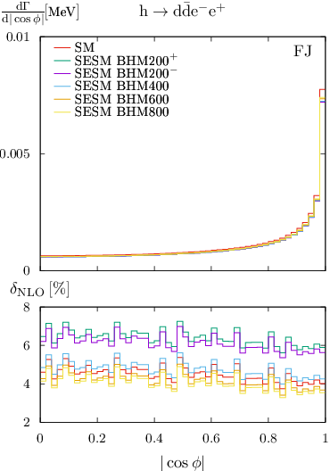
The left panel shows the differential width with respect to the invariant mass of the quark pair around the Z-boson peak. Below the peak, positive NLO corrections are driven by photon radiation from the final-state quarks. Compared to the leptonic case, the radiative tail is less pronounced due to the smaller charge factor of the quarks. Since all the gluons are recombined with the quark pair, gluon radiation does not contribute to the tail [51]. The presence of the singlet does not induce any shape distortion with respect to the SM distribution, and the difference between each SESM scenario and the SM equals the difference obtained for the corresponding integrated result.

The right panel of Fig. 23 shows the angular distribution in the cosine of the angle $\phi$ between the two Z-boson decay planes. For events without gluon radiation, the final-state quarks are identified with two jets. When gluon radiation occurs, the two QCD partons with the smallest invariant mass are recombined into a single jet, so that we always obtain events with two outgoing jets. Since the jets cannot be distinguished, any observable must be invariant under the exchange of the two jets, and the cosine of $\phi$ can be reconstructed only up to a sign. Thus, in the figure, it is defined by [51]

|\cos\phi|=\left|\frac{\left(\left(\mathbf{k}_{\text{jet}_{1}}+\mathbf{k}_{\text{jet}_{2}}\right)\times\mathbf{k}_{1}\right)\left(\mathbf{k}_{\text{jet}_{1}}\times\mathbf{k}_{\text{jet}_{2}}\right)}{|\left(\mathbf{k}_{\text{jet}_{1}}+\mathbf{k}_{\text{jet}_{2}}\right)\times\mathbf{k}_{1}|\,|\mathbf{k}_{\text{jet}_{1}}\times\mathbf{k}_{\text{jet}_{2}}|}\right|.

(7.16)

Note that, in the binning of the distribution, $\cos\phi$ is used instead of $\phi$ , so that the result looks different from the leptonic case reported in Fig. 21. The difference between the SESM and the SM is given by an offset, which depends on the considered scenario and is equal to the difference obtained for the corresponding integrated results.

In Fig. 24 invariant-mass and angular distributions for the charged-current final state $\nu_{\text{e}}{\text{e}^{+}}\text{d}\bar{\text{u}}$ are illustrated, including both EW and QCD corrections.

In the left panel, the invariant-mass distribution displays the W-boson peak, and the radiative tail induced by photon radiation can be observed. As observed in the leptonic case, there is no shape difference between the SM and the considered SESM distributions, and the difference in the normalization equals the relative difference obtained for the integrated decay widths. The angular distribution, reported in the right panel of Fig. 24, shows the cosine of the angle between the electron and the hadronically decaying W boson, in the Higgs rest frame. The NLO corrections slightly deform the distribution, but there is no difference in the distortion induced by the SESM and the SM. The difference between the two equals the difference encountered for the integrated results.

In general, we observe that the presence of the singlet does not change the shape of the SM distributions. Consequently, the study of differential distributions is not helpful to discriminate the SESM from the SM. The difference between the models is given by a different normalization in the distributions and equals the relative difference observed for the integrated decay widths. Similar results were obtained for the THDM in Ref. [56].

8 Conclusions

To explore the nature of EW symmetry breaking at the LHC, precise theory predictions are needed. This is valid not only within the SM, but also for its extensions, since BSM physics might show small deviations from SM predictions, below the $10\%$ level. Precision is also required in case of new discoveries, as different BSM theories lead to comparable effects, and a very high accuracy would be necessary to tell the right theoretical framework underlying the newly-observed states.

In this paper, we have considered a SESM characterized by a $\mathbb{Z}_{2}$ -invariant Lagrangian and non-vanishing vev both for the $\text{SU}(2)_{\scriptscriptstyle\text{W}}$ doublet and the real singlet scalar field. The model provides two Higgs bosons, which couple to the SM fields with the same couplings of the SM Higgs, rescaled by the sine or cosine of a mixing angle $\alpha$ . We parametrize the extended Higgs sector by the mass $M_{\text{H}}$ of the heavy Higgs boson, the mixing angle $\alpha$ , and the scalar self-coupling $\lambda_{12}$ connecting the scalar singlet and doublet. The renormalization of the theory has been performed adopting two schemes, in which the renormalized parameters $\alpha$ and $\lambda_{12}$ are defined by $\overline{\text{MS}}$ conditions, since these parameters are not directly experimentally accessible. In both schemes, all the quantities other than $\alpha$ and $\lambda_{12}$ are renormalized using OS conditions. In the first scheme the renormalized tadpoles are set to zero, as it is customary in OS renormalization schemes. This scheme introduces gauge dependences in the parametrization of observables by input parameters if $\overline{\text{MS}}$ parameters are involved, and thus should be used only within a fixed gauge. In the second scheme, following a prescription suggested by Fleischer and Jegerlehner, gauge dependences are avoided by setting unrenormalized (bare) tadpoles to zero, so that all relations between bare parameters of the theory are gauge independent.

Identifying the lighter Higgs boson h with the observed Higgs boson of mass $125\,\,\mathrm{GeV}$ , we have computed NLO EW and QCD corrections to the decays $\text{h}\to\text{W}\text{W}/\text{Z}\text{Z}\to 4\,$ fermions. Using the Mathematica package FeynRules, we have implemented the SESM into a FeynArts model file including the expressions of the renormalization constants, so that the model file can be used to perform NLO computations within the two considered renormalization schemes. Employing FeynArts and FormCalc, the model file has been used to produce Fortran code for the numerical computation of the matrix elements for the decays $\text{h}\to\text{W}\text{W}/\text{Z}\text{Z}\to 4\,$ fermions. The Fortran routines have been embedded in Prophecy4f to extend the capabilities of the Monte Carlo generator, which allows now for the computation of observables relevant for the Higgs decays to four fermions in the SESM at NLO.

The class of decay processes $\text{h}\to\text{W}\text{W}/\text{Z}\text{Z}\to 4\,$ fermions played a central role in the discovery of the Higgs boson and is important for the accurate characterization of the Higgs particle. We have analyzed the decays for some SESM benchmark scenarios proposed in the literature. For each scenario, we have computed the total decay width $\Gamma_{\text{h}\to 4f}$ for the decay of the light Higgs boson into four fermions and studied the dependence of the results on the renormalization scale $\mu_{\text{r}}$ , solving the RGE for the $\overline{\text{MS}}$ parameters $\alpha$ and $\lambda_{12}$ . We observe that the inclusion of NLO corrections drastically reduces the scale dependence and, consequently, the related theoretical uncertainty. Changing the scale up and down by factors of two, reduces the scale uncertainty of $\Gamma_{\text{h}\to 4f}$ typically from $\mathrel{\raisebox{-3.00003pt}{$\stackrel{{\scriptstyle\displaystyle<}}{{\sim}}$}}3{-}4\%$ at LO to only $\mathrel{\raisebox{-3.00003pt}{$\stackrel{{\scriptstyle\displaystyle<}}{{\sim}}$}}0.5\%$ at NLO.

All these analyses have been performed using both renormalization schemes, properly converting the numerical input values between the two schemes in order to ensure a consistent comparison between the predictions obtained for specific scenarios. To this end, we have investigated the conversion of the mixing angle $\alpha$ between renormalization schemes and found sizeable effects which become large when approaching non-perturbative regimes. The inclusion of NLO corrections improves the agreement between the results computed in the two schemes, i.e. the renormalization scheme dependence is reduced at NLO. In the considered scenarios, the scheme dependence at the central scale typically reduces from $\sim 1\%$ at LO to $\mathrel{\raisebox{-3.00003pt}{$\stackrel{{\scriptstyle\displaystyle<}}{{\sim}}$}}0.1\%$ at NLO. Note that the inclusion of conversion effects is essential in a consistent comparison of NLO predictions obtained in the two schemes.

Comparing the NLO decay widths $\Gamma_{\text{h}\to 4f}$ in the SESM with the corresponding quantities in the SM, we find deviations from the SM that reach about $-7\%$ in the scenarios BHM200^± with a heavy Higgs boson of mass $200\,\,\mathrm{GeV}$ . The NLO corrections are typically about $5{-}10\%$ , but only $1{-}2\%$ of those are due to effects beyond the SM. For higher values of the heavy mass $M_{\text{H}}$ , the (absolute values of the) deviations from the SM become smaller. Differential distributions have been produced for the SESM scenarios and compared to the SM case, and no distortions are observed on top of the SM shapes. The only observed difference is given by a constant offset, implying that differential distributions are not helpful to observe traces of the SESM.

Both the FeynArts model file and the new version of Prophecy4f are ready for further applications and can be obtained from the authors upon request.

Acknowledgements

We thank the Research Training Group GRK 2044 of the German Research Foundation (DFG) for funding and support and acknowledge support by the state of Baden-Württemberg through bwHPC and the DFG through grant no INST 39/963-1 FUGG. Moreover, M.B. and S.D. acknowledge the Research Executive Agency (REA) of the European Union for funding this work through the Grant Agreement PITN-GA-2012-316704 (“HiggsTools”).

Appendix

Appendix A Results for the scenario BHM200^-

The results for benchmark scenario BHM200^-, defined by the input values given in Table 2, are very similar to the results obtained for the scenarios BHM200⁺ and BHM600 (see Sects. 7.1 and 7.2); the most important of them are collected in this appendix.

In Fig. 26 we show the running of the parameters defined by $\overline{\text{MS}}$ conditions. Compared to the scenario BHM200⁺, the scale dependence of $s_{\alpha}$ in the FJ scheme is reduced. The scale dependence of the inclusive decay width $\Gamma_{\text{h}\to 4f}$ is shown in Fig. 26. The plot on the left is obtained using $\overline{\text{MS}}$ (FJ) input parameters converted to the FJ ( $\overline{\text{MS}}$ ) scheme at the scale $\mu_{0}=M_{\text{h}}$ . Dashed and solid lines correspond to LO and NLO (EW + QCD) results, respectively. Including NLO corrections, scale and scheme dependence are strongly reduced.

The total decay width $\Gamma_{\text{h}\to 4f}$ , the relative NLO corrections, and the deviations from the SM are shown respectively in Figs. 29, 29, and 29 as functions of $s_{\alpha}$ . The values of $M_{\text{H}}$ and $\lambda_{12}$ are fixed according to scenario BHM200^-. The plots on the left (right) are obtained using the $\overline{\text{MS}}$ (FJ) input scheme and converting $s_{\alpha}$ to the FJ ( $\overline{\text{MS}}$ ) scheme. LO and NLO (EW + QCD) results are represented, respectively, by dashed and solid lines. Where relevant, green lines represent the SM value. The vertical dashed lines at $s_{\alpha}\sim-0.05$ mark the maximal $s_{\alpha}$ value for which the perturbativity constraints (6.6) are fulfilled. The agreement between the two schemes improves after including NLO corrections. Quantitatively, the scale dependence of $\Gamma_{\text{h}\to 4f}$ (by scale variations of factors $2$ and $1/2$ ) reduces from $\sim 3{-}4\%$ at LO to $\sim 0.4\%$ at NLO in the ${\overline{\text{MS}}}$ scheme, and from $\sim 0.7\%$ at LO to $\mathrel{\raisebox{-3.00003pt}{$\stackrel{{\scriptstyle\displaystyle<}}{{\sim}}$}}0.1\%$ at NLO in the FJ scheme, reflecting the difference in the running of $\alpha$ in this scenario. The scheme dependence at the central scale reduces from $\sim 0.7\%$ at LO to $\mathrel{\raisebox{-3.00003pt}{$\stackrel{{\scriptstyle\displaystyle<}}{{\sim}}$}}0.1\%$ at NLO.

Appendix B Results for the scenario BHM400

In this appendix we show results for the scenario BHM400, defined by the input values given in Table 2. The calculations and the results are very similar to the ones described in Sects. 7.1 and 7.2 for the scenarios BHM200⁺ and BHM600, respectively, thus we do not discuss the details again.

The conversions of the mixing angle from the $\overline{\text{MS}}$ to the FJ scheme, and vice versa, are computed for $M_{\text{H}}$ and $|\lambda_{12}|$ values corresponding to the scenario BHM400 and shown in Fig. 32. The sign of $\lambda_{12}$ is fixed according to the sign of $s_{\alpha}$ on the $x$ -axis, as indicated in the figure. Red and blue lines correspond, respectively, to the complete and linearized solutions of Eq. 7.6. For values of $s_{\alpha}$ in the dark-gray area, the perturbativity constraints (6.6) are violated. The light-gray areas denote where the vacuum stability condition (2.16) is violated, or where the sign of $s_{\alpha}$ is flipped by the conversion (and becomes inconsistent with the sign of $\lambda_{12}$ ). The conversion effects are in general small and become larger when approaching the non-perturbative region.

The running of the parameters defined by ${\overline{\text{MS}}}$ renormalization conditions is shown, for the scenario BHM400, in Fig. 32. The scale dependence of the mixing angle is more accentuate in the FJ scheme, while the running of $\lambda_{12}$ is very similar in the two renormalization schemes.

In Fig. 32, we show the renormalization scale dependence of the $\text{h}\to 4f$ decay width. The left (right) panel is obtained using $\overline{\text{MS}}$ (FJ) input parameters and converting to the FJ ( $\overline{\text{MS}}$ ) scheme at the scale $\mu_{0}=M_{\text{h}}$ . Dashed lines correspond to LO results, solid lines include NLO EW+QCD contributions. Both scale and scheme dependence are reduced by the inclusion of NLO corrections. The scale dependence of the width reduces from $\sim 0.5\%$ at LO to $\sim 0.1\%$ at NLO in the ${\overline{\text{MS}}}$ scheme, and from $\sim 2\%$ at LO to $\sim 0.2\%$ at NLO in the FJ scheme, while the scheme dependence at the central scale is $\sim 0.2\%$ at LO and $\mathrel{\raisebox{-3.00003pt}{$\stackrel{{\scriptstyle\displaystyle<}}{{\sim}}$}}0.1\%$ at NLO.

Figures 35, 35, and 35 show, respectively, the absolute values, the relative NLO corrections, and the deviations from the SM for the decay width $\Gamma_{\text{h}\to 4f}$ in the SESM as functions of $s_{\alpha}$ . The parameters $M_{\text{H}}$ and $\lambda_{12}$ are fixed according to scenario BHM400. The plots on the left (right) are obtained using the $\overline{\text{MS}}$ (FJ) input scheme and converting $s_{\alpha}$ to the FJ ( $\overline{\text{MS}}$ ) scheme. As usual, dashed and solid lines represent, respectively, LO and NLO EW+QCD results. Where relevant, the SM result is reported in green. The dashed vertical line marks the minimal $s_{\alpha}$ value for which the perturbativity constraints (6.6) are fulfilled. The inclusion of NLO corrections improves the agreement between the results computed in the two schemes. For $s_{\alpha}=0.26$ , corresponding to the scenario BHM400, the decay width deviates $6{-}7\%$ from the SM value, slightly depending on the input scheme used.

References

[1] ATLAS Collaboration, G. Aad et al., Observation of a new particle in the search for the Standard Model Higgs boson with the ATLAS detector at the LHC, Phys. Lett. B716 (2012) 1–29, [arXiv:1207.7214].
[2] CMS Collaboration, S. Chatrchyan et al., Observation of a new boson at a mass of 125 GeV with the CMS experiment at the LHC, Phys. Lett. B716 (2012) 30–61, [arXiv:1207.7235].
[3] LHC Higgs Cross Section Working Group Collaboration, D. de Florian et al., Handbook of LHC Higgs Cross Sections: 4. Deciphering the Nature of the Higgs Sector, arXiv:1610.07922.
[4] M. Boggia et al., The HiggsTools Handbook: Concepts and observables for deciphering the Nature of the Higgs Sector, arXiv:1711.09875.
[5] V. Silveira and A. Zee, Scalar Phantoms, Phys. Lett. 161B (1985) 136–140.
[6] A. Hill and J. J. van der Bij, Strongly interacting singlet-doublet Higgs model, Phys. Rev. D36 (1987) 3463–3473.
[7] M. J. G. Veltman and F. J. Yndurain, Radiative corrections to $WW$ scattering, Nucl. Phys. B325 (1989) 1–17.
[8] J. McDonald, Gauge singlet scalars as cold dark matter, Phys. Rev. D50 (1994) 3637–3649, [hep-ph/0702143].
[9] M. C. Bento, O. Bertolami, R. Rosenfeld, and L. Teodoro, Selfinteracting dark matter and invisibly decaying Higgs, Phys. Rev. D62 (2000) 041302, [astro-ph/0003350].
[10] C. P. Burgess, M. Pospelov, and T. ter Veldhuis, The Minimal model of nonbaryonic dark matter: A Singlet scalar, Nucl. Phys. B619 (2001) 709–728, [hep-ph/0011335].
[11] H. Davoudiasl, R. Kitano, T. Li, and H. Murayama, The New minimal standard model, Phys. Lett. B609 (2005) 117–123, [hep-ph/0405097].
[12] R. M. Schabinger and J. D. Wells, A Minimal spontaneously broken hidden sector and its impact on Higgs boson physics at the large hadron collider, Phys. Rev. D72 (2005) 093007, [hep-ph/0509209].
[13] J. J. van der Bij, The Minimal non-minimal standard model, Phys. Lett. B636 (2006) 56–59, [hep-ph/0603082].
[14] B. Patt and F. Wilczek, Higgs-field portal into hidden sectors, hep-ph/0605188.
[15] D. G. Cerdeno, A. Dedes, and T. E. J. Underwood, The Minimal Phantom Sector of the Standard Model: Higgs Phenomenology and Dirac Leptogenesis, JHEP 09 (2006) 067, [hep-ph/0607157].
[16] A. Kusenko, Sterile neutrinos, dark matter, and the pulsar velocities in models with a Higgs singlet, Phys. Rev. Lett. 97 (2006) 241301, [hep-ph/0609081].
[17] V. Barger, P. Langacker, M. McCaskey, M. J. Ramsey-Musolf, and G. Shaughnessy, LHC Phenomenology of an Extended Standard Model with a Real Scalar Singlet, Phys. Rev. D77 (2008) 035005, [arXiv:0706.4311].
[18] V. Barger, P. Langacker, M. McCaskey, M. Ramsey-Musolf, and G. Shaughnessy, Complex Singlet Extension of the Standard Model, Phys. Rev. D79 (2009) 015018, [arXiv:0811.0393].
[19] X.-G. He, T. Li, X.-Q. Li, J. Tandean, and H.-C. Tsai, Constraints on Scalar Dark Matter from Direct Experimental Searches, Phys. Rev. D79 (2009) 023521, [arXiv:0811.0658].
[20] M. Gonderinger, Y. Li, H. Patel, and M. J. Ramsey-Musolf, Vacuum Stability, Perturbativity, and Scalar Singlet Dark Matter, JHEP 01 (2010) 053, [arXiv:0910.3167].
[21] S. Andreas, C. Arina, T. Hambye, F.-S. Ling, and M. H. G. Tytgat, A light scalar WIMP through the Higgs portal and CoGeNT, Phys. Rev. D82 (2010) 043522, [arXiv:1003.2595].
[22] Y. Mambrini, Higgs searches and singlet scalar dark matter: Combined constraints from XENON 100 and the LHC, Phys. Rev. D84 (2011) 115017, [arXiv:1108.0671].
[23] X.-G. He, B. Ren, and J. Tandean, Hints of Standard Model Higgs Boson at the LHC and Light Dark Matter Searches, Phys. Rev. D85 (2012) 093019, [arXiv:1112.6364].
[24] S. Profumo, M. J. Ramsey-Musolf, and G. Shaughnessy, Singlet Higgs phenomenology and the electroweak phase transition, JHEP 08 (2007) 010, [arXiv:0705.2425].
[25] J. R. Espinosa, T. Konstandin, and F. Riva, Strong Electroweak Phase Transitions in the Standard Model with a Singlet, Nucl. Phys. B854 (2012) 592–630, [arXiv:1107.5441].
[26] V. Barger, D. J. H. Chung, A. J. Long, and L.-T. Wang, Strongly First Order Phase Transitions Near an Enhanced Discrete Symmetry Point, Phys. Lett. B710 (2012) 1–7, [arXiv:1112.5460].
[27] A. Datta and A. Raychaudhuri, Next-to-minimal Higgs: Mass bounds and search prospects, Phys. Rev. D57 (1998) 2940–2948, [hep-ph/9708444].
[28] D. O’Connell, M. J. Ramsey-Musolf, and M. B. Wise, Minimal Extension of the Standard Model Scalar Sector, Phys. Rev. D75 (2007) 037701, [hep-ph/0611014].
[29] C. Englert, T. Plehn, D. Zerwas, and P. M. Zerwas, Exploring the Higgs portal, Phys. Lett. B703 (2011) 298–305, [arXiv:1106.3097].
[30] A. Djouadi, O. Lebedev, Y. Mambrini, and J. Quevillon, Implications of LHC searches for Higgs–portal dark matter, Phys. Lett. B709 (2012) 65–69, [arXiv:1112.3299].
[31] R. S. Gupta and J. D. Wells, Higgs boson search significance deformations due to mixed-in scalars, Phys. Lett. B710 (2012) 154–158, [arXiv:1110.0824].
[32] R. Coimbra, M. O. P. Sampaio, and R. Santos, ScannerS: Constraining the phase diagram of a complex scalar singlet at the LHC, Eur. Phys. J. C73 (2013) 2428, [arXiv:1301.2599].
[33] G. M. Pruna and T. Robens, Higgs singlet extension parameter space in the light of the LHC discovery, Phys. Rev. D88 (2013), no. 11 115012, [arXiv:1303.1150].
[34] R. Costa, A. P. Morais, M. O. P. Sampaio, and R. Santos, Two-loop stability of a complex singlet extended Standard Model, Phys. Rev. D92 (2015) 025024, [arXiv:1411.4048].
[35] T. Robens and T. Stefaniak, Status of the Higgs Singlet Extension of the Standard Model after LHC Run 1, Eur. Phys. J. C75 (2015) 104, [arXiv:1501.02234].
[36] A. Falkowski, C. Gross, and O. Lebedev, A second Higgs from the Higgs portal, JHEP 05 (2015) 057, [arXiv:1502.01361].
[37] T. Robens and T. Stefaniak, LHC Benchmark Scenarios for the Real Higgs Singlet Extension of the Standard Model, Eur. Phys. J. C76 (2016), no. 5 268, [arXiv:1601.07880].
[38] J. A. Casas, D. G. Cerdeño, J. M. Moreno, and J. Quilis, Reopening the Higgs portal for single scalar dark matter, JHEP 05 (2017) 036, [arXiv:1701.08134].
[39] J. Fleischer and F. Jegerlehner, Radiative Corrections to Higgs Decays in the Extended Weinberg-Salam Model, Phys. Rev. D23 (1981) 2001–2026.
[40] S. Actis, A. Ferroglia, M. Passera, and G. Passarino, Two-Loop Renormalization in the Standard Model. Part I: Prolegomena, Nucl. Phys. B777 (2007) 1–34, [hep-ph/0612122].
[41] M. Krause, R. Lorenz, M. Mühlleitner, R. Santos, and H. Ziesche, Gauge-independent Renormalization of the 2-Higgs-Doublet Model, JHEP 09 (2016) 143, [arXiv:1605.04853].
[42] A. Denner, L. Jenniches, J.-N. Lang, and C. Sturm, Gauge-independent $\overline{MS}$ renormalization in the 2HDM, JHEP 09 (2016) 115, [arXiv:1607.07352].
[43] L. Altenkamp, S. Dittmaier, and H. Rzehak, Renormalization schemes for the Two-Higgs-Doublet Model and applications to $h\to WW/ZZ\to 4$ fermions, JHEP 09 (2017) 134, [arXiv:1704.02645].
[44] A. Denner, J.-N. Lang, and S. Uccirati, NLO electroweak corrections in extended Higgs Sectors with RECOLA2, JHEP 07 (2017) 087, [arXiv:1705.06053].
[45] S. Kanemura, M. Kikuchi, and K. Yagyu, Radiative corrections to the Higgs boson couplings in the model with an additional real singlet scalar field, Nucl. Phys. B907 (2016) 286–322, [arXiv:1511.06211].
[46] F. Bojarski, G. Chalons, D. Lopez-Val, and T. Robens, Heavy to light Higgs boson decays at NLO in the Singlet Extension of the Standard Model, JHEP 02 (2016) 147, [arXiv:1511.08120].
[47] S. Kanemura, M. Kikuchi, and K. Yagyu, One-loop corrections to the Higgs self-couplings in the singlet extension, Nucl. Phys. B917 (2017) 154–177, [arXiv:1608.01582].
[48] S. Kanemura, M. Kikuchi, K. Sakurai, and K. Yagyu, Gauge invariant one-loop corrections to Higgs boson couplings in non-minimal Higgs models, Phys. Rev. D96 (2017), no. 3 035014, [arXiv:1705.05399].
[49] A. Denner, G. Weiglein, and S. Dittmaier, Gauge invariance of green functions: Background field method versus pinch technique, Phys. Lett. B333 (1994) 420–426, [hep-ph/9406204].
[50] A. Denner, G. Weiglein, and S. Dittmaier, Application of the background field method to the electroweak standard model, Nucl. Phys. B440 (1995) 95–128, [hep-ph/9410338].
[51] A. Bredenstein, A. Denner, S. Dittmaier, and M. M. Weber, Radiative corrections to the semileptonic and hadronic Higgs-boson decays $H\to WW/ZZ\to 4$ fermions, JHEP 02 (2007) 080, [hep-ph/0611234].
[52] A. Bredenstein, A. Denner, S. Dittmaier, and M. M. Weber, Precision calculations for the Higgs decays $H\to ZZ/WW\to 4$ leptons, Nucl. Phys. Proc. Suppl. 160 (2006) 131–135, [hep-ph/0607060]. [,131(2006)].
[53] A. Bredenstein, A. Denner, S. Dittmaier, and M. M. Weber, Precise predictions for the Higgs-boson decay $H\to WW/ZZ\to 4$ leptons, Phys. Rev. D74 (2006) 013004, [hep-ph/0604011].
[54] S. Boselli, C. M. Carloni Calame, G. Montagna, O. Nicrosini, and F. Piccinini, Higgs boson decay into four leptons at NLOPS electroweak accuracy, JHEP 06 (2015) 023, [arXiv:1503.07394].
[55] A. Denner, et al., Higgs Production and Decay with a Fourth Standard-Model-Like Fermion Generation, Eur. Phys. J. C72 (2012) 1992, [arXiv:1111.6395].
[56] L. Altenkamp, S. Dittmaier, and H. Rzehak, Precision calculations for $h\to WW/ZZ\to 4$ fermions in the Two-Higgs-Doublet Model with PROPHECY4F, arXiv:1710.07598.
[57] N. D. Christensen and C. Duhr, FeynRules - Feynman rules made easy, Comput. Phys. Commun. 180 (2009) 1614–1641, [arXiv:0806.4194].
[58] A. Alloul, N. D. Christensen, C. Degrande, C. Duhr, and B. Fuks, FeynRules 2.0 - A complete toolbox for tree-level phenomenology, Comput. Phys. Commun. 185 (2014) 2250–2300, [arXiv:1310.1921].
[59] T. Hahn, Generating Feynman diagrams and amplitudes with FeynArts 3, Comput. Phys. Commun. 140 (2001) 418–431, [hep-ph/0012260].
[60] T. Hahn and M. Perez-Victoria, Automatized one loop calculations in four-dimensions and D-dimensions, Comput. Phys. Commun. 118 (1999) 153–165, [hep-ph/9807565].
[61] R. K. Ellis, W. J. Stirling, and B. R. Webber, QCD and collider physics, Camb. Monogr. Part. Phys. Nucl. Phys. Cosmol. 8 (1996) 1–435.
[62] A. Denner, Techniques for calculation of electroweak radiative corrections at the one loop level and results for W physics at LEP-200, Fortsch. Phys. 41 (1993) 307–420, [arXiv:0709.1075].
[63] M. Böhm, H. Spiesberger, and W. Hollik, On the One Loop Renormalization of the Electroweak Standard Model and Its Application to Leptonic Processes, Fortsch. Phys. 34 (1986) 687–751.
[64] J. F. Gunion, H. E. Haber, G. L. Kane, and S. Dawson, The Higgs Hunter’s Guide, Front. Phys. 80 (2000) 1–404.
[65] A. Denner, E. Kraus, and M. Roth, Physical renormalization condition for the quark mixing matrix, Phys. Rev. D70 (2004) 033002, [hep-ph/0402130].
[66] B. A. Kniehl and A. Sirlin, A Novel Formulation of Cabibbo-Kobayashi-Maskawa Matrix Renormalization, Phys. Lett. B673 (2009) 208–210, [arXiv:0901.0114].
[67] A. Freitas and D. Stöckinger, Gauge dependence and renormalization of tan beta in the MSSM, Phys. Rev. D66 (2002) 095014, [hep-ph/0205281].
[68] A. Denner, S. Dittmaier, M. Roth, and D. Wackeroth, Predictions for all processes $e^{+}e^{-}\to 4$ fermions $+\gamma$ , Nucl. Phys. B560 (1999) 33–65, [hep-ph/9904472].
[69] A. Denner, S. Dittmaier, M. Roth, and L. H. Wieders, Complete electroweak O(alpha) corrections to charged-current $e^{+}e^{-}\to 4$ fermion processes, Phys. Lett. B612 (2005) 223–232, [hep-ph/0502063]. [Erratum: Phys. Lett.B704,667(2011)].
[70] A. Denner, S. Dittmaier, M. Roth, and L. H. Wieders, Electroweak corrections to charged-current $e^{+}e^{-}\to 4$ fermion processes: Technical details and further results, Nucl. Phys. B724 (2005) 247–294, [hep-ph/0505042]. [Erratum: Nucl. Phys.B854,504(2012)].
[71] A. Denner, S. Dittmaier, and L. Hofer, Collier: a fortran-based Complex One-Loop LIbrary in Extended Regularizations, Comput. Phys. Commun. 212 (2017) 220–238, [arXiv:1604.06792].
[72] S. Catani and M. H. Seymour, A General algorithm for calculating jet cross-sections in NLO QCD, Nucl. Phys. B485 (1997) 291–419, [hep-ph/9605323]. [Erratum: Nucl. Phys.B510,503(1998)].
[73] S. Dittmaier, A General approach to photon radiation off fermions, Nucl. Phys. B565 (2000) 69–122, [hep-ph/9904440].
[74] S. Dittmaier, A. Kabelschacht, and T. Kasprzik, Polarized QED splittings of massive fermions and dipole subtraction for non-collinear-safe observables, Nucl. Phys. B800 (2008) 146–189, [arXiv:0802.1405].
[75] LHC Higgs Cross Section Working Group Collaboration, S. Dittmaier et al., Handbook of LHC Higgs Cross Sections: 1. Inclusive Observables, arXiv:1101.0593.
[76] LHC Higgs Cross Section Working Group Collaboration, S. Dittmaier et al., Handbook of LHC Higgs Cross Sections: 2. Differential Distributions, arXiv:1201.3084.
[77] A. Sirlin, Radiative Corrections in the SU(2)-L x U(1) Theory: A Simple Renormalization Framework, Phys. Rev. D22 (1980) 971–981.
[78] D. López-Val and T. Robens, $\Delta$ r and the W-boson mass in the singlet extension of the standard model, Phys. Rev. D90 (2014) 114018, [arXiv:1406.1043].
[79] J. Küblbeck, M. Böhm, and A. Denner, Feyn Arts: Computer Algebraic Generation of Feynman Graphs and Amplitudes, Comput. Phys. Commun. 60 (1990) 165–180.
[80] ATLAS, CMS Collaboration, G. Aad et al., Combined Measurement of the Higgs Boson Mass in $pp$ Collisions at $\sqrt{s}=7$ and 8 TeV with the ATLAS and CMS Experiments, Phys. Rev. Lett. 114 (2015) 191803, [arXiv:1503.07589].
[81] Particle Data Group Collaboration, K. A. Olive et al., Review of Particle Physics, Chin. Phys. C38 (2014) 090001.
[82] R. Costa, M. Mühlleitner, M. O. P. Sampaio, and R. Santos, Singlet Extensions of the Standard Model at LHC Run 2: Benchmarks and Comparison with the NMSSM, JHEP 06 (2016) 034, [arXiv:1512.05355].
[83] C. A. Nelson, Correlation Between Decay Planes in Higgs Boson Decays Into $W$ Pair (Into $Z$ Pair), Phys. Rev. D37 (1988) 1220.
[84] A. Soni and R. M. Xu, Probing CP violation via Higgs decays to four leptons, Phys. Rev. D48 (1993) 5259–5263, [hep-ph/9301225].
[85] D. Chang, W.-Y. Keung, and I. Phillips, CP odd correlation in the decay of neutral Higgs boson into Z Z, W+ W-, or t anti-t, Phys. Rev. D48 (1993) 3225–3234, [hep-ph/9303226].
[86] A. Skjold and P. Osland, Angular and energy correlations in Higgs decay, Phys. Lett. B311 (1993) 261–265, [hep-ph/9303294].
[87] C. P. Buszello, I. Fleck, P. Marquard, and J. J. van der Bij, Prospective analysis of spin- and CP-sensitive variables in $H\to ZZ\to l_{1}^{+}l_{1}^{-}l_{2}^{+}l_{2}^{-}$ at the LHC, Eur. Phys. J. C32 (2004) 209–219, [hep-ph/0212396].
[88] T. Arens and L. M. Sehgal, Energy spectra and energy correlations in the decay $H\to ZZ\to\mu^{+}\mu^{-}\mu^{+}\mu^{-}$ , Z. Phys. C66 (1995) 89–94, [hep-ph/9409396].
[89] S. Y. Choi, D. J. Miller, M. M. Mühlleitner, and P. M. Zerwas, Identifying the Higgs spin and parity in decays to Z pairs, Phys. Lett. B553 (2003) 61–71, [hep-ph/0210077].
[90] S. Boselli, et al., Higgs decay into four charged leptons in the presence of dimension-six operators, arXiv:1703.06667.