The cylinder of a relation and generalized versions of the Nerve Theorem

The mapping cylinder $M(f)$ of a map $f:X\to Y$ between topological spaces is a tool that allows one to replace, up to homotopy, any continuous function $f$ by a nice inclusion, namely the cofibration $i:X\hookrightarrow M(f)$. The analogue of this construction in the context of posets, called the non-Hausdorff mapping cylinder, was introduced in [3] to study simple homotopy theory of polyhedra using the topology and combinatorics of finite topological spaces. The (non-Hausdorff) mapping cylinder $B(f)$ of an order preserving map $f:X\to Y$ between posets has similar properties as its classical analogue: $B(f)$ deformation retracts onto $Y$ (when they are viewed as finite topological spaces) and the inclusion $i:X\hookrightarrow B(f)$ satisfies nice properties. In [2] Barmak used the poset version of the mapping cylinder to give an alternative and simple proof of Quillen’s Theorem A for posets and to derive stronger formulations of the Nerve Theorem and other related results.

An order preserving map $f:X\to Y$ is a particular case of a relation ${\mathcal{R}}\subseteq X\times Y$ (a subset of the Cartesian product of the underlying sets) and it is natural to ask whether there exists a general construction of a cylinder of a relation that coincides with $B(f)$ in the case that the relation is the one induced by a poset map $f$. In this article we define the cylinder $B({\mathcal{R}})$ of any relation ${\mathcal{R}}\subseteq X\times Y$ and study its homotopical properties. Of course one cannot expect that $B({\mathcal{R}})$ preserves the homotopy type of $Y$ for a general relation ${\mathcal{R}}$ but we will show that this is the case when the relation satisfies good local properties (see Proposition 2.5). Analogously, under symmetric local hypotheses one can show that $B({\mathcal{R}})$ preserves the homotopy type of $X$ (Proposition 2.4). As an immediate consequence we obtain a generalization of Quillen’s Theorem A for relations (Theorem 2.6). When the relation is the one induced by an order preserving map $f:X\to Y$, Theorem 2.6 is precisely Quillen’s Theorem A for posets.

The Nerve Theorem, due to Borsuk [5], with alternative versions by Leray [11], Weil [18] and McCord [13], and more recently Björner [4] and Barmak [2], is a powerful tool widely used in Topology, Combinatorics, and, in the last years, in Computational and Applied Topology (see [6, 8, 9, 14]). The theorem essentially affirms that under certain hypotheses on a given space $X$, the nerve of a cover has the same homotopy type as $X$, provided that the cover is good. Which means that the intersection of any subfamily of the cover is either empty or contractible. However the requirement of being a good cover is somewhat restrictive and not always convenient. In Section 3 we prove generalizations of this theorem for not necessarily good covers. This is accomplished by using a formulation of the classical theorem in terms of posets (Theorem 3.2). The generalized versions of the Nerve Theorem are deduced by applying Theorem 2.6 to suitable relations.

Suppose that $K$ is a simplicial complex and ${\mathcal{U}}=\{L_{i}\}_{i\in I}$ is a cover of $K$ by subcomplexes, such that the intersections are not necessarily connected but the connected components of the non-empty intersections are contractible (this kind of situation appears for example in the study of point cloud data [6, 8, 16]). In this case the usual nerve ${\mathscr{N}}({\mathcal{U}})$ is not in general homotopy equivalent to $K$. In Section 3 we introduce the completion of the nerve $\hat{{\mathscr{N}}}({\mathcal{U}})$, which is a regular CW-complex (not necessarily a simplicial complex) built from the connected components of the non-empty intersections. Corollary 3.10 shows that the completion has the same homotopy type as $K$.

Given a finite simplicial complex $K$ (or more generally, a finite regular CW-complex), its face poset will be denoted by ${\mathcal{X}}(K)$. This is the poset of simplices (or cells) of $K$ ordered by inclusion. Conversely, given a finite poset $X$, ${\mathcal{K}}(X)$ denotes its classifying space (also called the order complex). This is the simplicial complex whose simplices are the non-empty chains of $X$. A finite poset can be seen as a finite topological space whose open subsets are the downsets (see [1, 3, 12, 17]). Its topology is related to the topology of the order complex ${\mathcal{K}}(X)$ by means of the McCord map $\mu:{\mathcal{K}}(X)\to X$ which is a weak (homotopy) equivalence (i.e. a continuous map which induces isomorphisms in all homotopy groups) [12]. There exists also a weak equivalence $\tilde{\nu}:K\to{\mathcal{X}}(K)$ associated to the functor ${\mathcal{X}}$. Although in this article we will not adopt explicitly the finite space point of view, we will use reduction methods of finite spaces to study homotopy properties of posets and complexes. We recall below the reduction methods that we will use and fix some notations. For more details the reader may consult [1].

Given a finite poset $X$ and $x\in X$, we denote by $U_{x}\subseteq X$ the subposet of elements which are smaller than or equal to $x$ (this is the minimal open subset containing $x$, if we view $X$ as a finite space). Analogously, we denote by $F_{x}$ the subposet of elements of $X$ which are greater than or equal to $x$ (this corresponds to the closure of $\{x\}$ in the finite space $X$). When a point $x$ belongs to different posets $X,Y$, sometimes we write $U_{x}^{X},U_{x}^{Y}$ (resp. $F_{x}^{X},F_{x}^{Y}$) to distinguish whether the subposets are considered in $X$ or in $Y$.

Note that a poset $X$ is homotopically trivial (which means that all its homotopy groups are trivial) if and only if ${\mathcal{K}}(X)$ is a contractible polyhedron. A finite poset is called a finite model of a CW-complex $K$ if its order complex ${\mathcal{K}}(X)$ is homotopy equivalent to $K$. The first reduction method for finite spaces was introduced by Stong [17]. Given a finite poset $X$, an element $x\in X$ is called an up beat point if $\hat{F}_{x}=F_{x}\smallsetminus\{x\}$ has a minimum, i.e. there is a unique element $y\in X$ which covers $x$. Similarly $x$ is called a down beat point if $\hat{U}_{x}=U_{x}\smallsetminus\{x\}$ has maximum (there is a unique $y$ covered by $x$). If $x$ is a beat point (up or down), $X\smallsetminus\{x\}\subseteq X$ is a strong deformation retract. This reduction (i.e. the removing of the point $x$) is denoted by $X{\searrow\hskip-6.0pt\searrow\hskip 3.0pt}X\smallsetminus\{x\}$. Stong proved that a finite poset $X$ is contractible if and only if one can remove beat points from $X$, one by one, to obtain a poset with only one element (this is also called dismantlable, see for example [10]). If $X$ is contractible then it is homotopically trivial, but the converse does not hold (see [1, Section 1.3] for more details). Note that the classical Whitehead’s Theorem is not valid in the context of finite spaces (there are finite spaces which are weak equivalent but not homotopy equivalent).

The notion of collapse in the context of posets was introduced by Barmak and Minian in [3] and it corresponds to Whitehead’s notion of simplicial collapse [7, 19]. Recall that a simplex $\sigma$ of a simplicial complex $K$ is a free face of $K$ if there is a unique simplex $\tau\in K$ containing $\sigma$ properly. In that case, there is a collapse from $K$ to the subcomplex $L=K\setminus\{\sigma,\tau\}$ (this is denoted by $K{\hskip 2.0pt\searrow\hskip 3.0pt}L$), and two simplicial complexes $K,T$ are simple homotopy equivalent if one can obtain one from the other by performing collapses and expansions (we denote $K{\hskip 2.0pt\diagup\hskip-4.8pt\searrow\hskip 5.0pt}T$ following the standard notation). If $K{\hskip 2.0pt\diagup\hskip-4.8pt\searrow\hskip 5.0pt}T$, they are in particular homotopy equivalent. A point $x$ of a finite poset $X$ is a down weak point if $\hat{U}_{x}$ is contractible, and it is an up weak point if $\hat{F}_{x}$ is contractible. An elementary collapse is the deletion of a weak point. The inverse operation is called an elementary expansion. We say that $X$ collapses to $Y$ (or $Y$ expands to $X$), and write $X{\hskip 2.0pt\searrow\hskip 3.0pt}Y$, if there is a sequence of elementary collapses which starts in $X$ and ends in $Y$. A poset $X$ is said to be collapsible if it collapses to a point. Note that any beat point is in particular a weak point (since posets with maximum or minimum are contractible). Therefore if $X$ is a contractible poset then it is collapsible. In [1, Sections 4.2 and 4.3] there are various examples of collapsible posets which are not contractible. Finally, we say that $X$ is simply equivalent to $Y$ if there exists a sequence of collapses and expansions that starts in $X$ and ends in $Y$. This is denoted by $X{\hskip 2.0pt\diagup\hskip-4.8pt\searrow\hskip 5.0pt}Y$. In [3] it is proved that $X{\hskip 2.0pt\diagup\hskip-4.8pt\searrow\hskip 5.0pt}Y$ if and only if the associated order complexes are simple homotopy equivalent. Moreover, if $X{\hskip 2.0pt\searrow\hskip 3.0pt}Y$ then ${\mathcal{K}}(X)$ simplicially collapses to ${\mathcal{K}}(Y)$. Conversely, $K{\hskip 2.0pt\diagup\hskip-4.8pt\searrow\hskip 5.0pt}L$ if and only if ${\mathcal{X}}(K){\hskip 2.0pt\diagup\hskip-4.8pt\searrow\hskip 5.0pt}{\mathcal{X}}(L)$. It can be also shown that if $\hat{U}_{x}$ or $\hat{F}_{x}$ is a collapsible poset then ${\mathcal{K}}(X){\hskip 2.0pt\searrow\hskip 3.0pt}{\mathcal{K}}(X\smallsetminus\{x\})$ (see [3, Remark 4.3.1]).

Finally, an element $x\in X$ is called a $\gamma$-point if $\hat{U}_{x}$ or $\hat{F}_{x}$ is homotopically trivial. In [1] it is proved that, in this case, the inclusion induces a simple homotopy equivalence ${\mathcal{K}}(X){\hskip 2.0pt\diagup\hskip-4.8pt\searrow\hskip 5.0pt}{\mathcal{K}}(X\smallsetminus\{x\})$. This reduction in denoted by $X{\hskip 2.4pt\searrow\hskip-8.0pt^{\gamma}\hskip 5.0pt}X\smallsetminus\{x\}$.

The relationship between the homotopy theory and simple homotopy theory of posets and polyhedra is summarized in the following theorem. The proof can be found in [1, 3]. We will use this relationship throughout the paper to derive results on complexes using posets and vice-versa.

The opposite of a poset $X$ will be denoted by $X^{op}$. This is the poset with the same underlying set as $X$ but with the opposite partial order. Note that $X{\hskip 2.0pt\diagup\hskip-4.8pt\searrow\hskip 5.0pt}X^{op}$ since their order complexes are isomorphic. A linear extension of a poset $Y$ is a total ordering $y_{1},y_{2},\ldots,y_{r}$ of the elements of $Y$ such that, if $y_{i}\leq y_{j}$, then $i\leq j$.

The non-Hausdorff mapping cylinder of an order preserving map $f:X\rightarrow Y$ between finite posets is the poset $B(f)$ with underlying set the disjoint union $X\sqcup Y$, and order relation defined by keeping the original ordering in $X$ and $Y$, and setting for each $x\in X$ and $y\in Y$, $x\leq y$ in $B(f)$ if $f(x)\leq y$ in $Y$. The mapping cylinder $B(f)$ has similar properties as the classical mapping cylinder. It is not difficult to see that $B(f){\searrow\hskip-6.0pt\searrow\hskip 3.0pt}Y$ and therefore, to study homotopy properties of posets, one can replace any order preserving map $f:X\to Y$ by the inclusion $i:X\hookrightarrow B(f)$. Under nice properties on $f$, $B(f)$ has the same topological properties as $X$.

Given two finite posets $X$ and $Y$, a relation ${\mathcal{R}}\subseteq X\times Y$ will mean a relation between their underlying sets (i.e. a subset ${\mathcal{R}}\subseteq X\times Y$ of the Cartesian product). We write $x{\mathcal{R}}y$ if $(x,y)\in{\mathcal{R}}$.

For $A\subseteq X$ and $B\subseteq Y$, we set

Let $A$ be a subposet of $X$, we denote

The next results relate the homotopy properties of $B({\mathcal{R}})$ with those of $X$ and $Y$. As a corollary we obtain a generalization of Quillen’s Theorem A. The proofs are based on the standard reduction methods of finite spaces mentioned above.

Analogously one can prove the following.

As a corollary of the previous results we obtain a generalization of Quillen’s Theorem A for relations ${\mathcal{R}}\subseteq X\times Y$.

If ${\mathcal{R}}$ is the relation associated to an order preserving map $f:X\to Y$, then $\underline{{\mathcal{R}}^{-1}(U_{y})}=f^{-1}(U_{y})$ and $\overline{{\mathcal{R}}(F_{x})}=F^{Y}_{f(x)}$. Note that, for any $x$, $F^{Y}_{f(x)}$ is contractible since it has a minimum. Therefore, the hypotheses of Proposition 2.5 are automatically fulfilled and one can deduce Quillen’s Theorem A [15] (cf. [2, Thm.1.2]).

By relaxing the hypotheses on ${\mathcal{R}}$, we obtain weaker versions of Theorem 2.6.

Recall that the nerve of a family ${\mathcal{U}}=\{U_{i}\}_{i\in I}$ of subsets of a set $X$ is the simplicial complex ${\mathscr{N}}({\mathcal{U}})$ whose simplices are the finite subsets $J\subseteq I$ such that $\displaystyle\bigcap_{i\in J}U_{i}\neq\varnothing$.

There exist different versions of the Nerve Theorem, involving open sets of topological spaces, subcomplexes of CW-complexes, etc. We mention here one version suitable for our purposes (see [2]).

The previous theorem can be restated in terms of finite posets by means of the functors ${\mathcal{X}}$ and ${\mathcal{K}}$. The equivalence between both formulations follows from Theorem 2.1. Note that covers by subcomplexes correspond to open covers of posets. Recall that a subposet of a poset $X$ is open if it is a downset. Given an open cover ${\mathcal{U}}=\{U_{i}\}_{i\in I}$ of a finite poset $X$, we write ${\mathcal{X}}({\mathcal{U}})={\mathcal{X}}({\mathscr{N}}({\mathcal{U}}))$. Note that the elements of the poset ${\mathcal{X}}({\mathcal{U}})$ are the subsets $J\subseteq I$ and the partial order is given by the inclusion.

Covers satisfying the hypotheses of Theorem 3.1 or Theorem 3.2 are called good. We use the formulation of the Nerve Theorem in terms of posets and Theorem 2.6 to derive generalizations of the result for covers which are not necessarily good. We introduce first some notations.

Let ${\mathcal{U}}=\{U_{i}\}_{i\in I}$ be an open cover of $X$. Given $J\subseteq I$ we denote by $W_{J}$ the intersection $\bigcap_{i\in J}U_{i}$. Note that $W_{J}$ is open in $X$ for every $J\subseteq I$. We denote by ${\mathcal{X}}_{0}({\mathcal{U}})$ the subposet of ${\mathcal{X}}({\mathcal{U}})$ consisting of all $J\subseteq I$ such that $W_{J}$ is homotopically trivial. Note that ${\mathcal{X}}_{0}({\mathcal{U}})={\mathcal{X}}({\mathcal{U}})$ if and only if ${\mathcal{U}}$ is a good cover. If $x\in X$ we denote by $I_{x}$ the subposet of ${\mathcal{X}}_{0}({\mathcal{U}})$ consisting of all $J\in{\mathcal{X}}_{0}({\mathcal{U}})$ such that $x\in W_{J}$. Note that $I_{x}$ is open in ${\mathcal{X}}_{0}({\mathcal{U}})$.

By relaxing the hypothesis on the subposets $I_{x}$, one can obtain variations of Theorem 3.3 using Proposition 2.8.

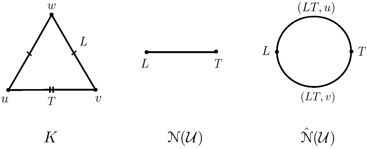
Suppose now that we are given a cover such that the intersections consist of disjoint unions of contractible subcomplexes (or homotopically trivial open subposets). For example, let $K$ be the boundary of the $2$-simplex with vertices $u,v,w$. Let $L$ be the subcomplex of $K$ consisting of the edges $\{u,w\}$ and $\{v,w\}$ and let $T$ be the edge $\{u,v\}$. The cover ${\mathcal{U}}=\{L,T\}$ is not good and clearly ${\mathscr{N}}({\mathcal{U}})$ is not homotopy equivalent to $K$, but the intersection $L\cap T$ is the union of two contractible subcomplexes (in this case, two points). We will show that in this situation we can replace the nerve ${\mathscr{N}}({\mathcal{U}})$ by a regular CW-complex $\hat{{\mathscr{N}}}({\mathcal{U}})$, which is homotopy equivalent to $K$ (see Example 3.11 below). The regular CW-complex $\hat{{\mathscr{N}}}({\mathcal{U}})$ will be the completion of the nerve. We study first the problem in the context of posets and then we derive the result for complexes.

From Theorem 3.8 we can derive a similar result for polyhedra. Note first that for any open cover ${\mathcal{U}}$ of a finite poset $X$, the completion $\hat{{\mathcal{X}}}({\mathcal{U}})$ is the face poset of a regular CW-complex (not necessarily a simplicial complex) whose cells are simplices. To see this, note that for every $(J,C)\in\hat{{\mathcal{X}}}({\mathcal{U}})$ the subposet $U_{(J,C)}$ is the face poset of a simplex (of dimension $\#J-1$) since for any $J^{\prime}\subseteq J$ there exists a unique component $C^{\prime}\subseteq W_{J^{\prime}}$ such that $C\subseteq C^{\prime}$. The $n$-cells of this regular CW-complex correspond to the connected components of the $W_{J}$ with $\#J=n+1$.

The following simple example illustrates the difference between the nerve and its completion.

References

- [1] Barmak, J.A. Algebraic topology of finite topological spaces and applications. Springer Lect. Notes Math. Vol. 2032 (2011).
- [2] Barmak, J.A. On Quillen’s Theorem A for posets. J. Combin. Theory Ser. A 118 (2011), 2445-2453.
- [3] Barmak, J.A.; Minian, E.G. Simple homotopy types and finite spaces. Adv. Math. 218 (2008), no. 1, 87-104.
- [4] Björner, A. Nerves, fibers and homotopy groups. J. Combin. Theory, Ser. A, 102 (2003), 88-93.
- [5] Borsuk, K. On the imbedding of systems of compacta in simplicial complexes. Fundamenta Mathematicae 35 (1948), 217-234.
- [6] Carlsson, G. Topology and data. Bull. Amer. Math. Soc. 46 (2009), 255-308.
- [7] Cohen, M.M. A Course in Simple Homotopy Theory. Springer-Verlag New York, Heidelberg, Berlin (1970).
- [8] de Silva, V.; Ghrist, R. Coverage in sensor networks via persistent homology. Algebr. Geom. Topol. 7 (2007), 339-358.
- [9] Dey, T.K.; Mémoli, F.; Wang, Y. Topological Analysis of Nerves, Reeb Spaces, Mappers, and Multiscale Mappers. SOCG 2017.
- [10] Duffus, D.; Rival, I. A structure theory for ordered sets. Discrete Math. 35 (1981), 53-118.
- [11] Leray, J. Sur la forme des espaces topologiques et sur les points fixes des représentations. J. Math. Pures Appl. 24 (1945) 95-167.
- [12] McCord, M.C. Singular homology groups and homotopy groups of finite topological spaces. Duke Math. J. 33 (1966), 465-474.
- [13] McCord, M.C. Homotopy type comparison of a space with complexes associated with its open covers. Proc. Amer. Math. Soc. 18 (1967), 705-708.
- [14] Nicolau, M.; Levine, A.J.; Carlsson, G.E. Topology based data analysis identifies a subgroup of breast cancers with a unique mutational profile and excellent survival. Proc. Natl. Acad. Sci. USA 108 (2011), 7265-7270.
- [15] Quillen, D. Homotopy properties of the poset of nontrivial p-subgroups of a group. Adv. Math. 28 (1978), 101-128.
- [16] Singh, G.; Mémoli, F.; Carlsson, G. Topological methods for the analysis of high dimensional data sets and 3d object recognition. SPBG (2007), 91-100.
- [17] Stong, R.E. Finite topological spaces. Trans. Amer. Math. Soc. 123 (1966), 325-340.
- [18] Weil, A. Sur les theoremes de de Rham Comment. Math. Helv. 26 (1952), 119-145.
- [19] Whitehead, J.H.C. Simplicial spaces, nuclei and m-groups. Proc. London Math. Soc. 45 (1939), 243-327.