Decoupled Learning for Factorial Marked Temporal Point Processes

Factorial point process refers to the processes in which event can be factorized into multiple markers. Except the job movement prediction and ICU department prediction mentioned in Introduction, many application cases can be described by the factorial point process, while haven’t been explored yet. For instance, a weather forecast containing temperature, humidity, precipitation, and wind can be seen as a factorial point process with $4$ markers, with each marker having discrete or continuous values. Obviously these factors affect each other, e.g. the humidity today is influenced by the precipitation and temperature in recent few days. The conventional marked point process could only model one of these factors using a single marker without considering the infectivity between these factors. A factorial point process with multiple markers for the event is essential.

Learning factorial point process is challenging. Taking job movement prediction with two markers company $c$ and position $p$ as example: to predict the probability of user $x$’s $n$-th job $(c_{n},p_{n})$, we need to learn a $4$-dimension tensor representing the impact of history companies $\{c_{i}\}_{i=1}^{n-1}$ on $c_{n}$ and $p_{n}$, the impact of history positions $\{p_{i}\}_{i=1}^{n-1}$ on $c_{n}$ and $p_{n}$, respectively. In point process, it means we need to learn a set of intensity functions including $\lambda(c,c)$, $\lambda(c,p)$, $\lambda(p,c)$ and $\lambda(p,p)$. This simple case considers no infectivity between different sequences, i.e., if we also consider the impact of another user y’s job movement on user $x$’s choice of $c_{n}$ and $p_{n}$, we would compute a $6$-dimension tensor to measure the complete infectivity, with two extra intensities $\lambda(y,c)$ and $\lambda(y,p)$.

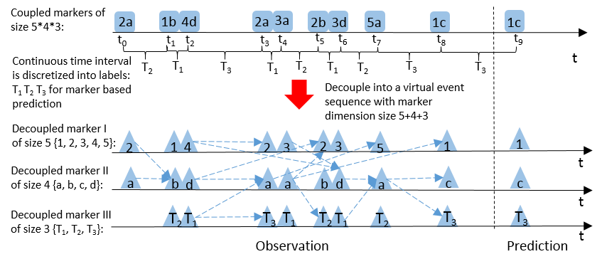
There are ways to simplify factorial point process learning, e.g. we can treat the combination of multiple factors as one marker, and use the conventional marked point process model, but this will lead to explosion of the size of infectivity matrix. In this paper, we explore a simple decoupling solution that decouple the factorial point process into separate models of different markers respectively. As shown in Fig.1 for the instance of $2$ markers $c$ and $p$, we decouple the original infectivity matrix into smaller one by introducing $4$ tensor variable $\bm{a}_{pp}$, $\bm{a}_{pc}$, $\bm{a}_{cp}$ and $\bm{a}_{cc}$. We will present the decoupled model in details in the following section.

More generally, we discuss the situation that event can be factorized into $Z$ markers $(m_{1},m_{2},\dots,m_{Z})$. Given event sequence $u$ with event marker $m_{i}=\{(m_{i,1},m_{i,2},\dots,m_{i,Z})\}$ for $m_{i,z}\in\{1,2,...,M_{z}\}$ where $z\in\{1,2,\dots,Z\}$, the intensity function of a conventional marked point process model for marker $m$ is defined by:

where $\bm{x}_{0}^{u}\in\mathbb{R}^{M}$ is the time-invariant features of sequence taker $u$ extracted from its profile, like Self-introduction of LinkedIn users or patients’ diagnose in MIMIC-II database, and $\bm{\theta}_{m}\in\mathbb{R}^{M}$ is the corresponding coefficients.

For the choice of the three functions $f$, $h$, $g$ in Eq. 1, there are many forms in the literature that can be abstracted by the above framework, and popular ones are depicted in Table I.

For marked point process model, when the marker contains multiple label dimensions, one major bottleneck is that this model involves the infectivity matrix $\bm{a}$ with size $(\prod_{z=1}^{Z}M_{z})\times(\prod_{z=1}^{Z}M_{z})$ to measure the directional effect between $m_{i}$ and $m_{j}$. More generally, the size of the infectivity matrix $\bm{a}$ is $O(n^{2Z})$ (assume all dimensions $M_{z}$ have same number of values by $n$), which incurs learning difficulty.

To mitigate the challenge for learning the above parameter matrix, especially when $\prod_{z=1}^{Z}M_{z}$ is large while the sequences are relatively short, we propose the decoupled factorial point process model to linearly decouple the above intensity function into $Z$ interdependent point processes $\lambda_{m_{z}}^{u}(t),z\in\{1,2,\dots,Z\}$ for the $z$-th marker as written by:

where $\bm{b}^{u}_{z_{i}}\in\{0,1\}^{M_{z}}$, $\bm{b}^{u}_{y_{j}}\in\{0,1\}^{M_{y}}$ is the binary indicators connecting through the influence of one’s former marker $z_{i}$ and markers $y_{j}$. Note the row vector $\bm{a}_{zz_{i}}\in\mathbb{R}^{1\times M_{z}}$ is the parameter for intra-influence within marker $\{z_{i}\}$, and $\bm{a}_{zy_{i}}\in\mathbb{R}^{1\times M_{y}}$ is for inter-influence between $z_{i}$ and $y_{i}$. The above vectors are illustrated in Fig.1 when $Z=2$, using notation $c$ as $z_{1}$ and $p$ as $z_{2}$.

In fact, function $f(\cdot)$, $g(\cdot)$, $h(\cdot)$ are predefined and some embodiments can be chosen from Table I. For the time being, we do not specify these functions while focus on solving the learning problem in a general setting.

A concrete example is presented in Fig.2. See the caption for more details.

Loss function for discriminative learning Based on the defined intensity function, we write out the probability $P(m,t|\mathcal{H}_{t}^{u})$ for event $m=\{m_{1},m_{2},\dots,m_{Z}\}$ happens at time $t$, conditioned on $u$’s history $\mathcal{H}_{t}^{u}$:

where $\lambda_{m}^{u}(t)$ is the event intensity, and $P(t|\mathcal{H}_{t}^{u})$ is the conditional probability that this event happens at time $t$ given history $\mathcal{H}_{t}^{u}$. $P(m|t,\mathcal{H}_{t}^{u})$ is the probability that the happened event is $m$ given current time $t$ and history $\mathcal{H}_{t}^{u}$.

Based on the above equation, most existing point process learning methods e.g. [12, 18, 19] fall into the generative learning framework aiming to maximize the joint probability of all observed events via a maximum likelihood estimator $\max_{\bm{\Theta}}\prod_{u,i}P(m_{i}^{u},t_{i}^{u}|\mathcal{H}_{t_{i}^{u}}^{u})$.

However, such an objective function is not tailored to the particular task at hand: instead of taking care of handling the posterior probability of the whole event sequence, we are more interested in predicting the next event and its mark information. To enable a more discriminative learning paradigm to boost the next event prediction accuracy, a recent work [17] suggests to focus on $P(m|t,\mathcal{H}_{t}^{u})$ instead of $P(m,t|\mathcal{H}_{t}^{u})$ as the loss function for learning.

In the decoupled point process model, the dependency between different markers has been measured by inter-influence parameters, i.e., the dependency between process $\lambda_{m_{z}}^{u}(t)$ for marker $m_{z}$ and process $\lambda_{m_{y}}^{u}(t)$ for marker $m_{y}$ have been measured by parameter $\bm{a}_{zy_{i}}$ and $\bm{a}_{yz_{i}}$ (see Eq. 2) in an independent fashion. In the same spirit, here we simplify the probability $P(m|t,\mathcal{H}_{t}^{u})$ by an independence assumption for marker $c$ and marker $p$:

where $P(m_{z}|t,\mathcal{H}_{t}^{u})$ is the normalized intensity function. This simplification leads to the following loss:

where $1\{statement\}$ is an indicator returning 1 if true, otherwise 0. $\bm{\Theta}=\{\bm{\Theta_{1}};\bm{\Theta_{2}};\dots;\bm{\Theta_{z}};\dots;\bm{\Theta_{Z}}\}\in\mathbb{R}^{(\sum_{z=1}^{Z}M_{z})\times(M+\sum_{z=1}^{Z}M_{z})}$ is the parameters whereby $\bm{\Theta_{c}}=[\bm{\theta_{z}}^{\top},\bm{a_{zz}},\bm{a_{zy}}|_{y=1,y\neq z}^{Z}]\in\mathbb{R}^{M_{z}\times(M+\sum_{z=1}^{Z}M_{z})}$

Sparse group regularization Since the model involves many parameters for learning, a natural idea is introducing sparsity to reduce the complexity. Incorporating both group sparsity and overall sparsity, we use a sparse group regularizer [15] as the regularization, a combination of $\ell_{1}$ regularization $\|\bm{\Theta}\|_{1}$ and a group lasso $\|\bm{\Theta}\|_{1,2}=\sum_{j=1}^{M+\sum_{z=1}^{Z}M_{z}}\|\theta_{j}\|_{2}$. The group lasso encourages the nonzero elements concentrated on a few columns in the whole matrix $\bm{\Theta}$, and the rest part is assumed to be zeros. The $\ell_{1}$ regularization encourages the whole matrix $\bm{\Theta}$ to be sparse. The behind rationale is that only a few profile features and event marker values will be the main contributor to the point process. This means only a few columns will be activated. As a result, the regularized objective is:

where $N=M+\sum_{z=1}^{Z}M_{z}$, $\bm{\Theta}\in\mathbb{R}^{(\sum_{z=1}^{Z}M_{z})\times N}$, $\lambda_{1}=\alpha\lambda$ and $\lambda_{2}=(1-\alpha)\lambda$, $\lambda$ is the regularization weight, $\alpha\in(0,1)$ controls the balance between overall and group sparsity.

First we review two soft-shrinkage operators [23] that solve the following two basic minimization problem, which will be used in our algorithm.

• •

  The minimization problem

  $$\arg\min_{\bm{\theta}\in\mathbb{R}^{p}}\{\|\bm{\theta}\|_{1}+\frac{u}{2}\|\bm{\theta}-\bm{r}\|^{2}\},$$

  with $u>0$, $\bm{\theta}\in\mathbb{R}^{p}$, $\bm{r}\in\mathbb{R}^{p}$, has a closed-form solution given by the soft-shrinkage operator $\bm{\textbf{shrink}_{1,2}}$ defined:

  $$\bm{\theta}^{*}=\text{shrink}_{1,2}(\bm{r},1/u)\triangleq\text{sign}(\bm{r})\cdot\max\{0,|\bm{r}|-1/u\},$$

  where $\text{sign}(\cdot)$ is the sign function.

• •

  The minimization problem

  $$\arg\min_{\bm{\theta}\in\mathbb{R}^{p}}\{\|\bm{\theta}\|_{2}+\frac{u}{2}\|\bm{\theta}-\bm{r}\|^{2}\},$$

  with $u>0$, $\bm{\theta}\in\mathbb{R}^{p}$, $\bm{r}\in\mathbb{R}^{p}$, has a closed-form solution given by the soft-shrinkage operator $\bm{\textbf{shrink}_{2,2}}$ defined:

  $$\bm{\theta}^{*}=\text{shrink}_{2,2}(\bm{r},1/u)\triangleq\frac{\bm{r}}{\|\bm{r}\|_{2}}\cdot\max\{0,\|\bm{r}\|_{2}-1/u\}.$$

To solve the minimization problem defined in Eq. 6 using ADMM solver, we add two auxiliary variables $\beta$, $\gamma$. The augmented Lagrangian function for Eq. 6 is $L_{u}^{s}(\bm{\Theta},\bm{\beta},\bm{\gamma})=$

where $\bm{\beta}=(\beta_{1},\beta_{2},\dots,\beta_{N})$, $\bm{\gamma}=(\gamma_{1},\gamma_{2},\dots,\gamma_{N})$, $\bm{\Theta}=(\theta_{1},\theta_{2},\dots,\theta_{N})$, and $\beta_{j},\gamma_{j},\theta_{j}\in\mathbb{R}^{C+P}$.

The iterative scheme is given by:

Therefore the optimization of Function 7 has been divided into two sub-problems defined as Eq. 8 and Eq. 9. While for Eq. 9, the update of $\bm{\gamma}$, it has a closed-form solution given by operator $\bm{\textbf{shrink}_{2,2}}$ as follows

where $\nu_{j}^{k}=(\bm{\Theta}^{k+1}-\bm{\beta}^{k}/u)_{j}$, $\mathcal{D}_{j}$ denotes the ball in $p_{j}$-dimension centered at 0 with radius $\lambda_{2}/u$ [23].

To solve Eq. 8 we define $g(\bm{\Theta})=L(\bm{\Theta})+\frac{u}{2}\|\bm{\Theta}-\bm{\gamma}^{k}-\bm{\beta}^{k}/u\|_{2}^{2}$, then $\bm{\Theta}^{k+1}$ can be obtained by solving $\bm{\Theta}=\arg\min\limits_{\bm{\Theta}}\{g(\bm{\Theta})+\lambda_{1}\|\bm{\Theta}\|_{1}\}$ through a FISTA method [22] with line search to compute the step size. The Algorithm is summarized in Alg.1

Based on the intensity function Eq. 2, the loss function Eq. 5, we show how to reformulate the learning of the decoupled point process as a multi-class Logistic Regression task. One obvious merit of this reformulation is the reuse of on-the-shelf LR solvers e.g. http://www.yelab.net/software/SLEP/ [24] with little parameter tuning. In contrast, the algorithm presented in Alg.2 involves more parameters and is more computational costive as shown in Fig.4 and Table II.

For event taker $u$ at time $t$, by separating the event taker $u$’s feature $\bm{f_{t}^{u}}=[x_{0}^{u}h(t),\sum_{i:t_{i}^{u}<t}b_{z_{i}}^{u}g(t,t_{i}),\sum_{y=1,y\neq z}^{Z}\sum_{j:t_{j}^{u}}b_{y_{j}}^{u}g(t,t_{j})]\in\mathbb{R}^{M+\sum_{z=1}^{Z}M_{z}}$ from the parameters $\bm{\Theta}_{z}$, the conditional intensity function in Eq. 2 can be written as:

Therefore the probability $P(p|t,\mathcal{H}_{t}^{u})$ can be written as:

This is exactly the same probability function of sample $\bm{f_{t}^{u}}$ belonging to class $m_{z}$ for a Softmax classifier of $M_{z}$ classes, and $\bm{\Theta}_{z}$ is the parameter.

Hence the log-loss function in Eq. 5 becomes:

which is the sum of $Z$ Softmax classifiers’ loss functions.

So far we have reformulated the decoupled learning of the factorial marked point process to the learning of $Z$ Softmax classifiers. For the $z$-th classifier, it takes $\bm{f_{t}^{u}}$ from the sample and classify it to one of $M_{z}$ markers $\hat{m_{z}}$. In the following experiments, we will show that the reformulated learning method in fact optimizes the same loss function as Alg.2.

After learning parameters $\bm{\Theta}=\{\bm{\Theta}_{z}|_{z=1}^{Z}\}$, we can predict the next event markers $m=\{\hat{m_{z}}|_{z=1}^{Z}\}$ at $t$, given history $\mathcal{H}_{t}^{u}$ by computing $P(m_{z}|t,\mathcal{H}_{t}^{u})$ (see Eq. 13). The predictions $\hat{c}$ and $\hat{m_{z}}$ are given by $\hat{m_{z}}=\arg\max_{\hat{m_{z}}\in M_{z}}P(m_{z}|t,\mathcal{H}_{t}^{u})$. It is important to note that though our model technically only issues discrete output as it is inherently a classification model, while in practice the future events’ timestamp can be predicted by an approximated discrete duration as done in our experiments. In this regard, we treat the future timestamp as a marker.

To verify the potential of the proposed model, we apply it to a LinkedIn-Career dataset crawled and de-identified from LinkedIn to predict user’s next company $\hat{c}$, next position $\hat{p}$ and duration $\hat{t}$ of current job; an ICU dataset extracted from public medical database MIMIC-II [8] to predict patient’s transition to the next ICU department $\hat{c}$ and duration of stay $\hat{p}$ in current department. Experiments are conducted under Ubuntu 64bit 16.04LTS, with i7-5557U 3.10GHz$\times$4 CPU and 8G RAM. For the convenience of replicating the experiments, the crawled de-identified LinkedIn-Career dataset and the code is available on Github²² 2 https://github.com/blade091shenwei/factorial-marked-point-process.

Dataset The LinkedIn-Career Dataset contains $5,006$ users crawled from information technology (IT) industry on LinkedIn (https://www.linkedin.com/), including their Self-introduction, Technical skills and Working Experience after de-identification preprocess. We collect samples in IT industry because: i) The staff turnover rate is high, which makes it easier to collect suitable samples; ii) The IT industry is most familiar to the authors, and our domain knowledge can help better curate the raw data. We extract profile features from users’ Self-introduction and Technical skills, and get users’ history company and position $\{(c_{i},p_{i})\}$ from Working Experience. After we exclude samples with zero job movement, we have a so-called LinkedIn-Career benchmark, involving 2,403 users, 57 IT companies, 10 kinds of positions and 4 kinds of durations. The dataset is to some extent representative for IT industry. For companies, we have large corporations like Google, Facebook, Microsoft and medium-sized enterprise like Adobe, Hulu, VMWare. For positions we have technical positions like engineer, senior engineer, tech lead, and management positions like manager, director, CEO. For durations we discretize the duration of stay in a position or company as temporary( within 1 year), short-term( 1-2 years), medium-term( 2-3 years) and long-term( more than 3 years). The goal is to predict user’s next company $\hat{c}$ from $C=57$ companies, next position $\hat{p}$ from $P=10$ positions and duration of stay in current company and position $\hat{t}$ from $T=4$ durations.

The ICU dataset contains $30,685$ patients from MIMIC-II database, including patients’ diagnose, treatment record, transition between different ICU departments and duration of stay in the departments. The goal is to predict patient’s next ICU department $\hat{c}$ from $C=8$ departments including Coronary care unit (CC), Anesthesia care unit (ACU), Fetal ICU (FICU), Cardiac surgery recovery unit (CSRU), Medical ICU (MICU), Trauma Surgical ICU (TSICU), Neonatal ICU (NICU), and General Ward (GW), and predict patient’s duration of stay $\hat{t}$ from $T=3$ kinds of duration including temporary( within 1 day), short-term( 1-5 days), and long-term (more than 5 days). The profile features are extracted from patients’ diagnose (ICD9 code of patients’ disease) and treatment record (nursing, medication, treatment).

Many peer methods are evaluated as follows:

Intensity function choices Our framework is tested by four point process embodiments namely: i) Mutually-corrected Processes (MCP), ii) Hawkes Process (HP), iii) Self-correcting Process (SCP) and iv) Modulated Poisson Process (MPP). Their characters are briefly compared in Table I. Note in our experiments, all these models are learned via the reformulated LR algorithm as described in Alg. 2.

Comparison to classic Logistic Regression We test a non-point process approach i.e. the plain LR. For the point process based LR solver, its input is $\bm{f_{t}^{u}}=[x_{0}^{u}h(t),\sum_{i:t_{i}^{u}<t}b_{z_{i}}^{u}g(t,t_{i}),\sum_{y=1,y\neq z}^{Z}\sum_{j:t_{j}^{u}}b_{y_{j}}^{u}g(t,t_{j})]$, while the plain LR involves the raw feature as $\bm{f^{u}}=[x_{0}^{u},b_{z_{I}}^{u},\sum_{y=1,y\neq z}^{Z}b_{y_{I}}^{u}]$, including user profile feature $x_{0}^{u}$, binary indicator $b_{z_{I}}^{u}$ and $\sum_{y=1,y\neq z}^{Z}b_{y_{I}}^{u}$ representing one’s current state without considering the history states.

Comparison to RNN and RMTPP We also experiment on RNN by treating the prediction task as a sequence classification problem. A dynamic RNN that can compute over sequences with variable length is implemented.

Moreover, to explore the effect of discretizing the time interval when making duration prediction, we also experiment on RMTPP (Recurrent Marked Temporal Point Process) proposed by [25]. Instead of predicting a discrete label for duration, it gives a continuous prediction result.

Prediction performance metrics We use prediction accuracy AC to evaluate the performance of the model with four variants $\mbox{AC}_{c}$, $\mbox{AC}_{p}$, $\mbox{AC}_{t}$, $\mbox{AC}_{cpt}$ to denote the prediction accuracy for state $c$ (i.e. # correct ones out of total predictions), state $p$, state $t$ and joint $c$,$p$,$t$ respectively.

To evaluate the performance of our discrete duration prediction compared with RMTPP, both MSE (Mean Squared Error) and AC are computed. To compute prediction MSE, the predicted discrete duration is substituted by the intermediate time point of the discrete intervals, e.g., 0.5 years for temporary stay, 1.5 years for short-term stay and 4 years for long-term stay. To compute prediction AC, the predicted continuous duration of RMTPP is discretized using the same criterion by the proposed model.

For LinkedIn-Career data, we further compute precision curve for the top-K position, company and duration predictions as shown in Fig. 3. These metrics are widely used for recommender system. In fact, as our model is for predicting the next company $\hat{c}$, next position $\hat{p}$ and duration $\hat{t}$ given career history $\mathcal{H}_{t}^{u}$, it can be used for recommending companies and posts at the predicted time period $\hat{t}$.

All the experimental results are obtained by 10-fold cross validation as commonly adopted like [26].

We are particularly interested in analyzing the following main bullets via empirical studies and quantitative results.

i) LR solver vs. ADMM solver To make a fair comparison, the LR solver and ADMM solver i.e. Alg.2 share the same initial parameter that initialized by a uniform distribution sampling from $(-1,1)$, and the running time and iteration count are the average of 10-fold cross validation. Table II compares LR solver and ADMM solver regarding with accuracy and time cost on the Dataset LinkedIn-Career and ICU. One can find the prediction accuracy is similar while the ADMM solver is more costive as we find it converges more slowly as shown in Fig.4. Also, as shown in Alg.2, it involves more hyper-parameters to tune and they have been tuned to their best performance. For comparison between the reformulated LR via the point process framework, and the raw LR using only user profile i.e. LR_np, we find the former outperforms in most cases in Table III and IV.

Comparing running time in Table II, the LR solver has better scalability than ADMM solver. This is because the ADMM solver is a general algorithm for convex optimization with sparse group regularization, while the LR solver works by a special design for the objectives that can be reformulated to Logistic Regression loss. Many algorithmic optimizations for Logistic Regression can be used in LR solver, like Efficient Projection in SLEP [24].

ii) Decoupled learning vs. RNN As shown in Table III and Table IV, the decoupled marked point process model has much better performance than RNN. This is because the next-event prediction task for relatively short sequences like dataset LinkedIn-Career and ICU is not a typical sequence classification task. We need to make prediction on every step of the sequence, rather than make prediction at the end of the whole sequence. That means for the end-to-end RNN sequence classification model, it needs to deal with sequences with considerably variable length, including a large number of sequences of length $1$.

We also compare the accuracy of RMTPP that makes continuous duration prediction, with decoupled model and general RNN in Table III and Table IV. Though the duration prediction accuracy of RMTPP is improved compared to general RNN, the decoupled model still have better performance.

To further verify the effect of discretizing the time interval when making duration prediction, the MSE of decoupled-MCP and RMTPP is also compared in Table V. Though it is a little tricky that discrete wrong prediction leads to smaller MSE than continuous wrong prediction, e.g., if a ground truth medium-term duration of 2.5 years is misclassified as long-term duration of 4 years for de-MCP, the RMTPP may gives a continuous prediction value of 10 years, the MSE of de-MCP is not only relatively but also absolutely small. It shows that the discretization of time interval is to some extent rational.

iii) Infectivity matrix decoupling vs. coupling Table III and Table IV also compare the performance of our decoupled model (see Eq. 2) against the raw coupled model (see Eq. 1), and the simplified model (single-dimension) when only marker $c$, $p$ or $t$ is considered. This boils down to the single-dimension case and the method is termed by uni-com, uni-pos and uni-dur for dataset LinkedIn-Career, and uni-duration and uni-transition for ICU respectively. While for uni-cpt, it involves no new model while uses the output of uni-c, uni-p and uni-t to combine them together as the joint prediction. It shows that the decoupled model consistently achieves the best performance, which perhaps is attributed to the reduction of model complexity given relatively limited training data.

Comparing the accuracies in Table III for dataset LinkedIn-Career and Table IV for dataset ICU, we can see that the improvement in accuracy of decoupled model compared to coupled model or single-dimension model, is more remarkable for LinkedIn-Career than that for ICU. The reason is that for LinkedIn-Career, the coupled state space is decoupled from $C\times P\times T=2280$ to $C+P+T=71$, and for ICU it is decoupled from $C\times T=24$ to $C+T=11$. The LinkedIn-Career dataset has a larger coupled state space than ICU. So when decoupled to smaller state spaces, the improvement for LinkedIn-Career is more notable than that for ICU.

iv) Choice of intensity function There are many popular intensity forms and some are listed in Table I. According to Table III and Table IV, the mutually-correcting process (MCP) consistently shows superior performance against other intensity function embodiments. This verifies two simple assumptions that i) the intensity tends to decrease for the moment the event happens, i.e., the desire for new job can be suppressed when a new job is fulfilled for job prediction, and patients’ demand for transition to next ICU department decrease after they move into a new department for ICU department transition prediction; ii) the probability of future events is influenced by the history events according to Table I, i.e., one’s transition possibility to new job is related to his/her history career experience, and patient’s future ICU department transition procedure is related to his/her history treatment.

v) Influence of sequence length To further explore the performance behavior, we experiment on short-sequences and long-sequences respectively on LinkedIn-Career³³ 3 ICU data is not included in the length test because $96\%$ of the patients in ICU have no more than three transitions.. Results in Table III show that the decoupled MCP algorithm has more advantage in long-sequence prediction, suggesting that the decoupled MCP can make better use of history information.

vi) Influence of sparsity To verify the effect of sparse group regularization, we compare the accuracy of the decoupled MCP model with different regularization settings, including without sparse regularization, with group lasso for group sparsity and with sparse group regularization (a combination of $\ell_{1}$ regularization and group lasso – see Eq. 6) for both overall sparsity and group sparsity. As shown in Table VI, the sparse group regularizer outperforms.

We also explore feature selection functionality by investigating the magnitudes of elements in matrix $\bm{\Theta}$. The element $\Theta_{ij}$ measures the influence of profile feature or marker $j$ to label $i$. Small (large) values indicate the corresponding features or markers have little (high) influence to label. For example, in LinkedIn-Career dataset, the numerical values in coefficient column vector corresponding to marker $engineer$ are all nonzero, showing that having a working experience as an $engineer$ is important in IT industry. For marker $director$, most of the elements in the corresponding coefficient column vector is zero except for the rows of positions $CEO$ and $founder$, suggesting an ascending career path in general.

References

- [1] D. Daley and D. Vere-Jones, An introduction to the theory of point processes: volume II: general theory and structure. Springer Science & Business Media, 2007.
- [2] A. Gelfand, P. Diggle, P. Guttorp, and M. Fuentes, Handbook of Spatial Statistics. CRC Press, 2010.
- [3] T. J. Liniger, “Multivariate hawkes processes,” PhD thesis, Swiss Federal Institute Of Technology, Zurich, 2009.
- [4] K. Zhou, H. Zha, and L. Song, “Learning social infectivity in sparse low-rank networks using multi-dimensional hawkes processes,” in AISTATS, 2013.
- [5] S. Xiao, J. Yan, X. Yang, H. Zha, and S. Chu, “Modeling the intensity function of point process via recurrent neural networks,” in AAAI, 2017.
- [6] Z. Ghahramani and M. I. Jordan, “Factorial hidden markov models,” in Advances in Neural Information Processing Systems, 1996, pp. 472–478.
- [7] A. G. Hawkes, “Spectra of some self-exciting and mutually exciting point processes,” Biometrika, 1971.
- [8] A. L. Goldberger, L. A. Amaral, L. Glass, J. M. Hausdorff, P. C. Ivanov, R. G. Mark, J. E. Mietus, G. B. Moody, C.-K. Peng, and H. E. Stanley, “Physiobank, physiotoolkit, and physionet components of a new research resource for complex physiologic signals,” Circulation, vol. 101, no. 23, pp. e215–e220, 2000.
- [9] Y. Ogata, “Statistical models for earthquake occurrences and residual analysis for point processes,” J. Amer. Statist. Assoc., vol. 83, no. 401, pp. 9–27, 1988.
- [10] ——, “Space-time point-process models for earthquake occurrences,” Annals of the Institute of Statistical Mathematics, vol. 50, pp. 379–402, 1998.
- [11] T. Ozaki, “Maximum likelihood estimation of hawkes’ self-exciting point processes,” Annals of the Institute of Statistical Mathematics, vol. 31, no. 1, pp. 145–155, 1979.
- [12] E. Lewis and E. Mohler, “A nonparametric em algorithm for multiscale hawkes processes,” Journal of Nonparametric Statistics, 2011.
- [13] A. Y. Ng, “Feature selection, l 1 vs. l 2 regularization, and rotational invariance,” in Proceedings of the twenty-first international conference on Machine learning. ACM, 2004, p. 78.
- [14] L. Meier, S. Van De Geer, and P. Bühlmann, “The group lasso for logistic regression,” Journal of the Royal Statistical Society: Series B (Statistical Methodology), vol. 70, no. 1, pp. 53–71, 2008.
- [15] N. Simon, J. Friedman, T. Hastie, and R. Tibshirani, “A sparse-group lasso,” Journal of Computational and Graphical Statistics, vol. 22, no. 2, pp. 231–245, 2013.
- [16] L. Li and H. Zha, “Learning parametric models for social infectivity in multi-dimensional hawkes processes,” in Twenty-Eighth AAAI Conference on Artificial Intelligence, 2014.
- [17] H. Xu, W. Wu, S. Nemati, and H. Zha, “Icu patient flow prediction via discriminative learning of mutually-correcting processes,” arXiv preprint arXiv:1602.05112, 2016.
- [18] K. Zhou, H. Zha, and L. Song, “Learning triggering kernels for multi-dimensional hawkes processes,” in ICML, 2013.
- [19] N. Du, Y. Wang, N. He, and L. Song, “Time-sensitive recommendation from recurrent user activities,” in NIPS, 2015.
- [20] C. Lloyd, T. Gunter, M. Osborne, and S. Roberts, “Variational inference for gaussian process modulated poisson processes,” in ICML, 2015.
- [21] V. Isham and M. Westcott, “A self-correcting point process,” Stochastic Processes and Their Applications, vol. 8, no. 3, pp. 335–347, 1979.
- [22] A. Beck and M. Teboulle, “A fast iterative shrinkage-thresholding algorithm for linear inverse problems,” SIAM journal on imaging sciences, vol. 2, no. 1, pp. 183–202, 2009.
- [23] D. L. Donoho, “De-noising by soft-thresholding,” IEEE transactions on information theory, vol. 41, no. 3, pp. 613–627, 1995.
- [24] J. Liu, S. Ji, and J. Ye, SLEP: Sparse Learning with Efficient Projections, Arizona State University, 2009. [Online]. Available: http://www.public.asu.edu/ jye02/Software/SLEP
- [25] N. Du, H. Dai, R. Trivedi, U. Upadhyay, M. Gomez-Rodriguez, and L. Song, “Recurrent marked temporal point processes: Embedding event history to vector,” in Proceedings of the 22nd ACM SIGKDD International Conference on Knowledge Discovery and Data Mining. ACM, 2016, pp. 1555–1564.
- [26] J. Yan, Y. Wang, K. Zhou, J. Huang, C. Tian, H. Zha, and W. Dong, “Towards effective prioritizing water pipe replacement and rehabilitation,” in IJCAI, 2013.
![[Uncaptioned image]](1801.06805v1/weichang.jpg) |
Weichang Wu received the B.S. degree in electronic engineering from Huazhong University of Science and Technology, Wu Han, China, in 2013. He is currently pursuing the Ph.D. degree with the Department of Electronic Engineering, Shanghai Jiao Tong University, Shanghai, China. His current research interests include data mining, especially medical information mining and disease modeling based on event sequence learning. |
![[Uncaptioned image]](1801.06805v1/junchi.jpg) |
Junchi Yan (M’10) is currently an Associate Professor with Shanghai Jiao Tong University. Before that, he was a Senior Research Staff Member and Principal Scientist for visual computing with IBM Research where he started his career since April 2011. He obtained the Ph.D. at the Department of Electronic Engineering of Shanghai Jiao Tong University, China. He received the ACM China Doctoral Dissertation Nomination Award and China Computer Federation Doctoral Dissertation Award. His research interests are machine learning and visual computing. He serves as an Associate Editor for IEEE ACCESS and on the executive board of ACM China Multimedia Chapter. |
![[Uncaptioned image]](1801.06805v1/xiaokang.jpg) |
Xiaokang Yang (M’00-SM’04) received the B. S. degree from Xiamen University, Xiamen, China, in 1994, the M. S. degree from Chinese Academy of Sciences in 1997, and the Ph.D. degree from Shanghai Jiao Tong University in 2000. He is currently a Distinguished Professor of School of Electronic Information and Electrical Engineering, Shanghai Jiao Tong University, Shanghai, China. His research interests include visual signal processing and communication, media analysis and retrieval, and pattern recognition. He serves as an Associate Editor of IEEE Transactions on Multimedia and an Associate Editor of IEEE Signal Processing Letters. |
![[Uncaptioned image]](1801.06805v1/hongyuan.jpg) |
Hongyuan Zha is a Professor at the School of Computational Science and Engineering, College of Computing, Georgia Institute of Technology and East China Normal University. He earned his PhD degree in scientific computing from Stanford University in 1993. Since then he has been working on information retrieval, machine learning applications and numerical methods. He is the recipient of the Leslie Fox Prize (1991, second prize) of the Institute of Mathematics and its Applications, the Outstanding Paper Awards of the 26th International Conference on Advances in Neural Information Processing Systems (NIPS 2013) and the Best Student Paper Award (advisor) of the 34th ACM SIGIR International Conference on Information Retrieval (SIGIR 2011). He was an Associate Editor of IEEE Transactions on Knowledge and Data Engineering. |