Using Deep Learning for Title-Based Semantic Subject Indexing to Reach Competitive Performance to Full-Text

Conference: The 18th ACM/IEEE Joint Conference on Digital Libraries; June 3–7, 2018; Fort Worth, TX, USAJCDL ’18: The 18th ACM/IEEE Joint Conference on Digital Libraries, June 3–7, 2018, Fort Worth, TX, USAPrice: 15.00DOI: 10.1145/3197026.3197039ISBN: 978-1-4503-5178-2/18/06CCS: Information systems Digital libraries and archivesCCS: Computing methodologies Neural networksCCS: Computing methodologies Natural language processing

Florian Mai Affiliation: Kiel University email: stu96542@informatik.uni-kiel.de , Lukas Galke Affiliation: Kiel University email: lga@informatik.uni-kiel.de and Ansgar Scherp Affiliation: Kiel University email: asc@informatik.uni-kiel.de

Abstract.

For (semi-)automated subject indexing systems in digital libraries, it is often more practical to use metadata such as the title of a publication instead of the full-text or the abstract. Therefore, it is desirable to have good text mining and text classification algorithms that operate well already on the title of a publication. So far, the classification performance on titles is not competitive with the performance on the full-texts if the same number of training samples is used for training. However, it is much easier to obtain title data in large quantities and to use it for training than full-text data. In this paper, we investigate the question how models obtained from training on increasing amounts of title training data compare to models from training on a constant number of full-texts. We evaluate this question on a large-scale dataset from the medical domain (PubMed) and from economics (EconBiz). In these datasets, the titles and annotations of millions of publications are available, and they outnumber the available full-texts by a factor of 20 and 15, respectively. To exploit these large amounts of data to their full potential, we develop three strong deep learning classifiers and evaluate their performance on the two datasets. The results are promising. On the EconBiz dataset, all three classifiers outperform their full-text counterparts by a large margin. The best title-based classifier outperforms the best full-text method by 9.4%. On the PubMed dataset, the best title-based method almost reaches the performance of the best full-text classifier, with a difference of only 2.9%.

Keywords:

Text classification; deep learning; digital libraries

1. Introduction

Semantic annotations are crucial for users of digital libraries as they enhance the search of scientific documents. Given the large amount of new publications, automatic annotation systems are a useful tool for human expert annotators working at digital libraries to classify the publications into categories from a (hierarchical) thesaurus. However, providing automated recommendations for subject indexing in such systems is a challenging task. This is partly due to the data from which recommendations may be generated. Often neither the full-text of a publication nor its abstract may be available. For instance, the digital library EconBiz contains only for 15% of the documents an abstract. Even when the content can be legally provided by the library to the end users, copyright laws or regulations of the publishers may prevent text mining. Moreover, collecting and processing PDFs where it is possible, e. g., for some Open Access documents, adds high computational requirements to the library. This puts annotation methods on demand that are based on data with better availability, such as the title. Previous work by Galke et al. (Galke et al., 2017a), however, has shown that title-based methods considerably fall behind full-text methods in terms of performance when the number of samples for training is equal. If our classifier was a human expert, this would not be a surprising result. A full-text contains more information and therefore also more indication of the publication’s topic. A human expert will always make better annotations based on the full-text. In fact, the annotations that are used as gold-standard for automated subject indexing experiments are often created based on the full-text.

However, we argue that machine learning algorithms work differently than a human. In contrast to a human, they often require hundreds of thousands or even millions of training data to yield satisfactory models (Brain and Webb, 1999). These amounts of data are not always available in the real world. One common reason is that human expertise is required for creating a large enough gold standard, which is expensive. For semantic subject indexing, the availability issues mentioned above do not only come into play at prediction time, i.e., when a machine learning model is used in a productive system, but also during training. In effect, methods based on the full-texts have drastically less training data available than methods based on titles. This raises the question if title-based methods can potentially narrow the performance gap to full-text methods by fully incorporating all training data available.

In this paper, we address this question. Formally, semantic indexing is framed as a multi-label classification problem, where a (commonly small) subset of labels has to be selected from a (relatively large) set of labels. From two digital libraries of scientific literature, PubMed and EconBiz, we have compiled an English full-text dataset and an English title dataset. Our compiled datasets are quite different with respect to their size. From PubMed, we extracted 12.83 million titles. For 5% of these a full-text is available (646k). From EconBiz, we extracted 1.06 million titles, of which approximately 7% have a full-text (71k). In order to fully utilize these large amounts of data, we develop and compare three different classifiers that have emerged from the deep learning community in recent years. Deep learning has advanced the state-of-the-art in many fields, such as vision, speech, and text (LeCun et al., 2015). These techniques are known to shine when a lot of training data is available. For text classification in particular, recent work (Zhang et al., 2015) suggests that deep learning starts to outperform strong traditional models when 650k or more training samples are available. The number of full-text in PubMed is right at the edge of this number, whereas EconBiz has far less full-texts, making these datasets an interesting and revealing choice. In natural language processing, different types of neural networks have been successfully employed on different tasks, but it is an open question whether convolutional neural networks (CNNs), recurrent neural networks (RNNs), or multi-layer-perceptrons (MLPs) are superior for text classification tasks. Therefore, we employ a representative of each type in our study. We compare them against another strong MLP baseline (Base-MLP), which has previously been shown to also outperform traditional bag-of-words classifiers such as SVMs, Naive Bayes, and kNN (Galke et al., 2017a). Since the label space in our datasets is very large, our study can be understood as eXtreme Multi-Label Classification (XMLC). Here, only few studies have leveraged deep learning techniques to tackle the considerably harder problem when the label space is large (Zhang et al., 2017; Liu et al., 2017). Hence, with our study, we contribute to the knowledge in this field, as well.

The results of our study indicate that title-based methods can match or even outperform the full-text performance when enough training data is available. On EconBiz, the best title classifier (MLP) performs on par with the best full-text classifier (MLP) when training with only 8 $\times$ as many titles as there are full-texts available. When all available titles are used (approximately 15 $\times$ more than full-texts), the title-based MLP outperforms its full-text counterpart by 9.4%. On the PubMed dataset, the best title method is the RNN, and it almost reaches the best full-text performance produced by an MLP. The gap is only as small as 2.9%. When using the same number of titles as full-texts are available, the gap in classification performance is 10.7%, indicating a considerable benefit from leveraging all title data. Generally, the MLP performs well, outperforming RNN and CNN in three out of the four combinations of the two datasets and title/full-text. It also consistently outperforms the baseline when all titles or full-texts are used. Moreover, our analysis suggests that our proposed classifiers are well-chosen for our study, because they benefit from increasing amounts of training data better than the baseline. The RNN performs rather poor on full-text, but shows strong performance on titles. While also yielding reasonably good results with CNN, it performs clearly below the other classifiers in all cases. This is a surprise, because a lot of the recent literature on large-scale text classification has focused on CNNs (e.g. (Zhang et al., 2015; Conneau et al., 2017; Le et al., 2018), also see Section 2). Thus, our results indicate that it may be worth it to shift the research focus more towards other types of neural networks for text classification.

Our contributions can be summarized as follows:

•

For the first time, we study the question whether title-based methods can reach the performance of full-text-based methods by exploiting the surplus of available training data.
•

We demonstrate that title-based methods are on par or even outperform full-text methods when the number of training samples is sufficiently large.
•

We develop and compare three strong classifiers for (extreme) multi-label text classification, contributing to the debate on which type of neural network is superior for text classification.

The remainder of the paper is structured as follows. In the subsequent section, we review relevant work on the comparison of short texts and full-text and on deep learning for text classification. In Section 3, we describe our deep learning models. We introduce the datasets and experimental setup in Section 4, and present the results in Section 5. We analyze and discuss the results in Section 6, before we conclude.

2. Related Work

In this section, we review previous literature relevant to our study. First, we discuss papers that compare performance on titles with performance on full-text. Next, we briefly discuss methods for multi-label text classification other than deep learning. Finally, we discuss current deep learning methods for text classification.

Title versus Full-Text

The work directly related to our study is the one by Galke et al. (Galke et al., 2017a). The authors compare titles with full-texts for multi-label text classification on four datasets. Two datasets consist of scientific publications and are therefore comparable to the datasets in this study. In their experiments, the authors used the same number of samples for the title-based methods and the full-text methods. They found that the title-based methods can yield reasonably good performance. However, the difference between title and full-text on the two scientific datasets is still 10% and 20% in favor of the full-text, respectively. The first dataset is from the economics domain, and it is an earlier version of the one used in this study. The second dataset is from the political sciences. In their comparison of classifiers, an MLP to which in this study we refer as Base-MLP, outperforms all other (non-neural) classifiers in 7 out of 8 combinations. All the presented classifiers are based on the bag-of-words (BoW) feature representation, a traditionally strong baseline for text classification that disregards word order. Due to clearly superior performance, Base-MLP can also be considered the best representative of traditional BoW models. We therefore report its performance as our baseline for all subsequently developed models.

The comparison of metadata vs. full-texts has also been studied for tasks other than document classification. Nascimento et al. (Nascimento et al., 2011) studied how well queries for web search can be generated from title, abstract, or body, respectively. These queries are then issued to Web information sources to retrieve papers for recommendation. In their experiments, abstracts yielded the best queries, closely followed by the body. The title clearly performs worse. On the contrary, Nishioka and Scherp (Nishioka and Scherp, 2016) have demonstrated that competitive paper recommendations to researchers based on their Twitter profile can be made by using only the title of the paper. This is achieved by their novel profiling method HCF-IDF, which is able to extract sufficient conceptual information from the title through spreading activation over a hierarchical knowledge base. Galke et al. (Galke et al., 2017b) use text embedding techniques for the information retrieval task and compare how well these techniques perform when the index is built upon the title, abstract, or full-text of the documents. Here, titles have demonstrated a clear advantage over abstract and full-text. Lastly, Hemminger et al. (Hemminger et al., 2007) compare full-text search with metadata search in the PubMed database, where full-text search yields better results.

Multi-label Text Classification

Text classification is a well-studied problem. k-Nearest-Neighbors and SVM are common choices for text classification (see e.g. (Joachims, 1998; Rubin et al., 2012; Große-Bölting et al., 2015)). However, kNN’s complexity grows in the number of training samples, which is problematic for the training sample sizes we consider in our study. SVMs do not provide a natural adaptation for multi-label classification. A binary relevance classification scheme, however, is impractical when the number of labels is large.

An active field of multi-label text classification research is the MeSH indexing community. This area is concerned with annotating PubMed articles with medical subject headings. BioASQ (Tsatsaronis et al., 2015) is a challenge that recently finished its 5th iteration. It has the goal to advance the state-of-the-art in MeSH indexing, and to this end provides large datasets for training. We acknowledge the significance of the MeSH indexing community, and in our study, we include the dataset from the latest iteration of the BioASQ challenge. However, many of the approaches successful at this challenge, including learning to rank (Huang et al., 2011; Liu et al., 2015; Mao and Lu, 2017) and pattern matching (Mork et al., 2014), make use of features tailored to the biomedical domain. Since in this paper, we study domain-independent methods for subject indexing in digital libraries, these methods are not appropriate.

Deep Learning for Text Classification

Some early works leverage neural networks for multi-label text classification. In order to capture label inter-dependencies, Zhang and Zhou (Zhang and Zhou, 2006) employ a pairwise ranking loss function for text classification. Nam et al. (Nam et al., 2014) show that replacing the ranking-loss with cross-entropy leads to faster convergence and overall better prediction performance. Furthermore, they are the first to incorporate some of the milestone advancements from the deep learning era like rectified linear units, dropout, and the smart optimizer AdaGrad.

In recent years, neural networks have become the state-of-the-art in multi-class text classification, outperforming traditional linear BoW models, in particular on very large datasets. On a diverse set of text classification datasets of rather small scale (up to 10.7k samples), neural networks have shown their capability to perform well. These include CNNs (Kim, 2014; Yin and Schütze, 2015) and RNNs (Tai et al., 2015), as well as a combination of both (Zhang et al., 2016).

Zhang et al. (Zhang et al., 2015) were the first to introduce several large-scale multi-class text classification datasets ranging from 120k to 3.6 million training samples. The number of classes ranges from two to 14. Zhang et al. proposed a deep, character-based convolutional neural network and compared it with a number of traditional models, including multinomial logistic regression based on bag-of-ngrams with TF-IDF, and deep learning models such as a Long Short-Term Memory network (LSTM) and word-based CNNs. The finding most relevant to our study is that traditional models tend to outperform the neural network architectures on the four relatively small datasets with 560k training samples or less, whereas on the remaining four datasets with 650k training samples or more their neural network approach is superior. Although these numbers may vary depending on the dataset and classification task at hand, this result is the main reason why we choose to employ deep learning techniques in our study.

Several studies employing deep learning on these datasets have followed. Conneau et al. (Conneau et al., 2017) draw inspiration from the computer vision community and improve the performance of character-based CNNs by increasing the depth. Le et al. (Le et al., 2018) put these results into perspective by demonstrating that a shallow, word-based CNN performs on par with these models or better. Therefore, we have limited our study to shallow, word-based CNNs. For text classification, it is an open question whether CNNs or RNNs are superior (Yin et al., 2017). Consequently, LSTMs had also some success on these large-scale datasets (Yang et al., 2016; Yogatama et al., 2017), as well as hybrid approaches (Xiao and Cho, 2016). Joulin et al. (Grave et al., 2017) demonstrated that even a linear MLP classifier can yield results competitive with non-linear deep learning methods while maintaining computational efficiency.

To the best of our knowledge, each of the neural network types MLP, CNN, and LSTM provide the current state-of-the-art on at least one of these large-scale datasets (as shown in the work by Le et al. (Le et al., 2018)). Hence, with our study we would like to contribute to this discussion by employing a representative of each of the neural network types.

Finally, due to the number of labels in our datasets, our study may be classified as XMLC. To the best of our knowledge, only two papers studied the application of deep learning to this setting (Zhang et al., 2017; Liu et al., 2017), from which we draw some inspiration for our models, which are described below.

3. Methods

In this section, we present three neural network architectures for text classification used in our study. In the design phase, we aimed at carefully developing the strongest representative of each of the most common types of neural networks, MLPs, CNNs, and RNNs¹¹ 1 For transparency, intermediate results of the design phase can be found in an extended version of the paper provided at https://github.com/florianmai/Quadflor.. Here, we only present the final architectures which are used in the experiments presented in Section 4. These architectures may differ depending on the dataset and type of text (title or full-text) they operate on. This is necessary to avoid a bias for either of the datasets or types of text. The output layer as well as the training procedure in our neural networks are the same for all neural network architectures presented here.

Below, we describe the training procedure, before we go into each neural network architecture up to the last hidden layer. For brevity, we omit a formal mathematical description of the models here.

3.1. Training Procedure

The semantic annotation task is formally a multi-labeling problem, where instead of belonging to exactly one class, each publication is assigned a set of labels. This is an important difference to most of the previous literature on text classification with large datasets. Binary Relevance is a common technique to adapt a classifier for a multi-labeling problem. However, this is a costly technique when the number of labels is high because it requires to train as many classifiers as there are labels. Neural networks have a more natural way to deal with multi-label classification, which is also made use of by Galke et al. (Galke et al., 2017a). For multi-class text classification, the softmax activation function is used at the output layer to obtain a probability distribution over the classes. For multi-label classification, however, the sigmoid activation can be employed to determine a probability $p_{l}$ for each label $l$ whether it should be assigned or not. The difference is that softmax regards all labels at once, while sigmoid makes an independent decision for each label. Finally, the binary decision whether label $l$ is assigned is made by checking whether $p_{l}$ exceeds a threshold $\theta$ .

Using Adam (Kingma and Ba, 2014), the networks are trained as to minimize the sum of all binary cross-entropy losses over all labels. This has shown to be superior to a ranking-based loss on multi-label text classification (Nam et al., 2014; Liu et al., 2017). Training is executed in mini-batches of size 256. We employ early stopping for regularization and as criterion to terminate training. The performance on the validation set is evaluated in terms of the sample-based $F_{1}$ -measure. Training is terminated when the validation score has not improved over the best reported score for 10 consecutive evaluations.

Since the output of the sigmoid activation function can be interpreted as the probability whether a label should be assigned, a typical choice for the threshold is $\theta=0.5$ . However, depending on the evaluation metric, dataset, or model that generates the assignment probabilities, this value does not necessarily yield optimal results. Unfortunately, finding a good value for $\theta$ can be computationally expensive, especially when the datasets are very large. Therefore, we use a heuristic that continuously adjusts the threshold during training. To this end, the evaluation on the validation set used for early stopping is also used to optimize $\theta$ .

Formally, we initially set $\theta_{0}:=0.2$ , which Galke et al. (Galke et al., 2017a) found to be a better threshold value than 0.5. After each validation step $i$ , where the classifier predicts a probability for each of the $\left|L\right|$ labels and each of the $n$ samples in the validation set, accumulated in $P_{i}\in(0,1)^{n\times|L|}$ , we set

\theta_{i}:=\argmax\limits_{\tilde{\theta}\in\{-k*\alpha+\theta_{i-1},\ldots,k*\alpha+\theta_{i-1}\}}F_{1}(P_{i};\tilde{\theta})

where $\alpha>0$ is the step size and $k$ controls the number of threshold values to check. This heuristic is based on the observation that the optimal choice for $\theta_{i}$ is in most cases in close proximity to the optimal choice of the previous evaluation step, $\theta_{i-1}$ . Since computing the $F_{1}$ score can be costly, we set $k=3$ and $\alpha=0.01$ to trade off granularity with speed.

In our preliminary experiments, this way of optimizing the threshold consistently yields good results, sometimes even better than when it is optimized manually.

3.2. Multi-Layer-Perceptron

Our baseline is a multi-layer-perceptron (MLP) described by Galke et al. (Galke et al., 2017a). It has one hidden layer with 1,000 units and rectifier activation and it takes a TF-IDF (Salton and Buckley, 1988) bag-of-unigrams as input. The bag-of-unigrams only contains the 25,000 most common unigrams, which we determined to be sufficient for the multi-labeling task. For regularization, dropout (Srivastava et al., 2014) is applied after the hidden layer with a keep probability of 0.5. We will refer to this baseline as Base-MLP.

We extend the MLP from Galke et al. (Galke et al., 2017a) by incorporating some techniques inspired from recent deep learning literature. The MLP architecture introduced in this study can be viewed as an adaptation of fastText (Grave et al., 2017) for multi-label classification. FastText is a linear BoW model enhanced with a feature sharing component (a hidden layer with identity activation) and local word order information (bigrams). We adopt this model by adding the 25,000 most common bi-grams in addition to the 25,000 most common unigrams. However, we found that omitting the non-linearity at the hidden layer rather hurts the classification performance considerably. Therefore, we keep the rectifier as a non-linear activation at the hidden layer.

In the introduction, it was mentioned that deep neural networks excel when the number of training samples is very large. This is because the representational power of neural networks increases as the number of parameters increases. This can be obtained by adding more layers or by adding more units to the existing layers. Additionally, deeper networks may be able to learn hierarchical representations of the input, as can be observed in the vision domain (He et al., 2016). However, deep networks are generally harder to train due to the vanishing and exploding gradient problems. We apply Batch Normalization (Ioffe and Szegedy, 2015) to our deep MLPs to alleviate those.

In summary, MLP differs from Base-MLP in that it incorporates bi-grams and uses multiple layers and Batch Normalization where appropriate.

3.3. Convolutional Neural Network

We present a CNN architecture whose core was introduced by Kim (Kim, 2014) for sentence classification and has since been repeatedly adopted and enhanced upon. We adopt and combine some of these enhancements for our model.

The CNN operates on word embeddings, which are initialized with a pretrained model but finetuned during training. As in Kim’s model, our CNN applies a 1D-convolution by sliding a window over the text in order to extract features at each position. These outputs are then transformed by a non-linear activation function (the detector). Commonly, the most salient position is selected by applying max-pooling after the detector stage. However, Liu et al. (Liu et al., 2017) instead split the output of the convolution into $p$ nearly equal chunks, and perform max-pooling on each chunk. Afterwards, the outputs of the pooling stages are concatenated. For $p=1$ , this is identical to Kim’s architecture.

Commonly, this process is repeated for multiple window sizes. The outputs of these processes are then concatenated before passing them to the next layer. For example, Kim’s CNN uses window sizes 3, 4, and 5, while Liu et al. use 2, 4, and 8. We experimentally determined that using 2, 3, 4, 5, and 8 yields to even better results.

In Kim’s model, the concatenated output of the pooling stages is directly propagated to the output layer. Liu et al. argue, however, that it is better to have an additional fully-connected layer with $n_{b}$ units, called the bottleneck layer, because it adds more representational power to the network through the increased depth.

Considering the complexity of our datasets and the number of training samples available, the question of increased capacity arises with CNNs. Similar to MLPs, an increase in capacity can be achieved either through wider convolutions (larger feature-map) or additional stacked layers of convolutions. Since a recent study by Le et al. (Le et al., 2018) has shown that depth does not yield improvement over shallow nets, we only consider the former approach.

3.4. Recurrent Neural Network

The Recurrent Neural Network (RNN) is a family of neural networks that was specifically designed for sequential input data. By maintaining a hidden state, the network is able to keep track of previous inputs. However, the vanilla RNN has difficulties keeping track of inputs that are far in the past. The LSTM (Hochreiter and Schmidhuber, 1997) was designed to alleviate this by explicitly modeling the control over whether the current hidden state shall be forgotten, updated, or kept. For this study, initially we use an LSTM that has already achieved good results for text classification in a study by Zhang et al. (Zhang et al., 2015). This LSTM is the “vanilla” version described in (Greff et al., 2017). Our final model, however, incorporates two techniques which have proven useful for NLP tasks in recent years, attention and bidirectionality (Young et al., 2017).

Since any RNN produces an output at every time step, the outputs have to be aggregated after processing the entire sequence, in order to pass a vector of fixed size to the next layer. We experimented with choosing the last output, computing the sum, computing the average, and computing a weighted average where the weights are determined by an attention mechanism as used by Yang et al. (Yang et al., 2016). While the benefit over the other aggregation methods is not large for titles, the attention mechanism consistently performs best. On full-texts, on the other hand, the difference is considerable. This is intuitive, because there is less need to focus on specific parts of the input if the input is as short as in a title.

In the same fashion as Yang et al. (Yang et al., 2016), we incorporate bidirectionality into our LSTM by concatenating at each time step the output of an LSTM that reads the input sequence from left to right, and an LSTM that reads the sequence in reverse order. This is a common technique to make the model aware of the entire sequence at every time step, and commonly boosts performance in text applications.

Again, we made some effort to investigate an increase in the capacity of the LSTM to account for the large number of training samples in our datasets. In the past, both increasing the memory cell size (the width) and stacking LSTMs on top of each other has been successful in some NLP tasks. For text classification, this has not been the case. The results of our experiments support this, where wider LSTMs are superior to stacked LSTMs, even when variational dropout (Gal and Ghahramani, 2016) is used.

4. Experimental Setup

Figure 1. We organize our dataset in several sub-datasets to perform an iterative evaluation. T1 and Full comprise of the same set of publications (all samples where a full-text is available), and is split into 10 folds in order to perform the same 10-fold cross-validation with titles and full-texts for a fair comparison. For T2, T4, T8, increasingly more titles that do not have a full-text are added for training, but are in each cross-validation step evaluated on the same test samples (highlighted in green for exemplification).

T_{all}

includes all title samples.

4.1. Datasets

We built English datasets from two digital libraries of scientific publications. EconBiz²² 2 https://www.econbiz.de/ is a search portal for economics and business studies. Currently, it contains 2,485,000 English publications, out of which 615k are open access. Many publications are annotated by experts with a variable number of subject headings (so-called subject indexing) taken from a standardized set, the ‘‘Thesaurus for Economics’’ (STW)³³ 3 http://zbw.eu/stw/version/latest/about. From all 2,485,000 English publications, we filtered the ones that have annotations and extracted their title. After deleting duplicates, 1,064,634 publications with annotations remain. Out of the 615k open access publications, the number of publications that have annotations and whose full-text can be downloaded and processed reduces to 70,619, which is 6.63% of all publications.

PubMed⁴⁴ 4 https://www.ncbi.nlm.nih.gov/pubmed/ is a search engine for biomedical and life science literature provided by the US National Library of Medicine. The publications found on PubMed are annotated with ‘‘Medical Subject Headings’’ (MeSH)⁵⁵ 5 https://www.nlm.nih.gov/mesh/meshhome.html by human curators. We obtained a dataset consisting of millions of publication metadata, including title and MeSH annotations, from the training set of the semantic indexing task of the BioASQ challenge 2017 (Tsatsaronis et al., 2015), which are all in English language. PubMed Central⁶⁶ 6 https://www.ncbi.nlm.nih.gov/pmc/ is an archive of full-texts of biomedical and life science literature provided by the US National Library of Medicine. It comprises 4.3 million publications, which can be accessed freely and which are mostly English. However, only 1.5 million are open access and therefore allow text mining. From this dataset, we computed the intersection with the publications obtained from the BioASQ challenge. After removing duplicates, 12,834,026 titles and 646,513 full-texts with respective annotations remain. Hence, 5.04% of the samples have a full-text.

Table 1 lists some characteristics of the two datasets, EconBiz and PubMed. In terms of combinatorial complexity, the PubMed dataset is a harder problem because the number of labels out of which to pick the annotations for a publication is much higher. Yet, due to the relatively large number of labels and small number of samples per label on average, both datasets can be considered as XMLC problems⁷⁷ 7 An overview of datasets commonly considered XMLC can be found at http://manikvarma.org/downloads/XC/XMLRepository.html.. The titles in PubMed contain on average more words than the publications’ titles in EconBiz. However, this fact is put into perspective considering that the titles in PubMed have on average more labels to be predicted than there are words in the title. Regarding the full-texts, the ratio of words/labels is approximately the same in both datasets. Another fact worth noting is that the titles corpora have on average one label less than the full-texts. This suggests that the label distributions in the title dataset and full-text dataset are quite different.

Table 1. Characteristics of EconBiz and PubMed datasets.

\left|D\right|

denotes the sample size,

\left|L\right|

denotes the number of labels used in the dataset,

d/l

is the average number of publications a label is assigned to.

l/d

is the average number of labels assigned to a publication.

\left|V\right|

is the size of the vocabulary and

w/d

denotes the average number of words per document.

	EconBiz (STW)		PubMed (MeSH)
	Title	Full-Text	Title	Full-Text
$\left\|D\right\|$	1,064,634	70,619	12,834,026	646,513
Size	78.8MB	6.27GB	1.32GB	20.06GB
$\left\|L\right\|$	5661	4849	27773	26276
$d/l$	819.1	75.8	5852.3	331.0
$l/d$	4.4	5.3	12.6	13.5
$\left\|V\right\|$	91,505	1,502,336	660,180	6,774,130
$w/d$	6.88	6694.4	9.6	2533.4

Please note that on both datasets, the set of titles is a superset of the set of full-texts.

4.2. Experiments

In order to assess how the title-based methods behave as more and more titles are considered for training, we create sub-datasets of the title datasets by iteratively adding more data. This is illustrated in Figure 1.

For a fair comparison of title and full-text performance, the trained model must be evaluated on the same data. To this end, we split the set of publications where a full-text is available into ten folds, and perform a 10-fold cross-validation. In each iteration, nine folds are selected for training, and one is selected for testing. From this training set, we randomly select 20% for the validation set for early stopping and adjusting the threshold, as described in Section 3.1. These comprise the data used for our experiments on full-text, and will be abbreviated as EconBiz Full and PubMed Full, respectively.

For the experiments on titles, the same publications from the 10-fold cross-validation are used for testing. However, the training set is iteratively extended with more samples from the titles dataset, so that the total number of training samples is always a power of two of the number of samples in the full-text experiment. In total, we conduct experiments on five title sub-datasets per domain: T1, T2, T4, T8, and $T_{all}$ . Here, Tx means that $x$ times as many title samples are used for training as there are full-text samples in the dataset. Lastly, $T_{all}$ contains all title samples from the dataset.

We run each of the four classifiers Base-MLP, MLP, CNN, and LSTM on all of the sub-datasets. In total, we run 48 cross-validations. Following Galke et al. (Galke et al., 2017a) who argue that the sample-based $F_{1}$ -metric best reflects how subject indexers work, we use this metric to report the results. We also use this metric for early stopping and threshold adjustment on the validation set. The sample-based $F_{1}$ -measure calculates the harmonic mean of precision and recall for each sample individually, and averages these scores over all samples.

4.3. Choice of Hyperparameters and Training

Since there are a lot of tunable hyperparameters involved in deep learning, tuning multiple hyperparameters at the same time can be very expensive, especially when the datasets are very large. On the other hand, fixing hyperparameters across all datasets and models would not be a fair approach in our study because the datasets and model architectures are very different and therefore may require very different hyperparameter settings. As a compromise, we decided to tune the hyperparameters for full-texts and titles separately in an incremental fashion on one fold. Here, we tuned one hyperparameter at a time and selected the locally best solution for full-text and titles, respectively. It is important to note that the parameters for titles were determined based on the performance on $T_{all}$ , and were adopted for all other title sub-datasets. On the one hand, this alleviates a lot of the computational cost and allows to compare the performance between title sub-datasets. On the other hand, especially the performance of smaller sub-datasets might be suboptimal due to overfitting. This must be kept in mind for analysis.

In our experiments involving the MLP, we use a one-layer MLP with 2,000 units and dropout with a keep probability of 0.5 after the hidden layer for all experiments. Only for the experiments on the PubMed titles, we use a two-layer MLP with 1,000 units each, and apply no dropout. Instead, we use Batch Normalization after each hidden layer. In all cases, the initial learning rate for Adam is set to 0.001.

In the CNN experiments, we use $p=3$ chunks and $n_{b}=1,000$ units at the bottleneck layer (Liu et al., 2017) for both full-text experiments. On titles, we do not perform chunking ( $p=1$ ), and use a bottleneck layer size of $n_{b}=500$ . The size of the feature map is set to 400 in all experiments except for PubMed Full, where we use 100. The keep probability is set to 0.75 in all cases, and the initial learning rate is 0.001.

We use a single-layer LSTM for all experiments. For both datasets, we determined 1,536 to be the best size for the memory cell when using titles. 1,024 units and 512 are used for PubMed Full and EconBiz Full, respectively. The keep probability is set to 0.75 in all experiments except for PubMed on titles, where we set it to 0.5. The initial learning rate is 0.01 for EconBiz Full and 0.001 in all other cases. Training is done with backpropagation through time by unrolling the LSTM until the end of the sequence.

We adopt the preprocessing and tokenization procedure of Galke et. al (Galke et al., 2017a). For the LSTM and CNN, we use 300-dimensional pretrained word embeddings obtained from training GloVe (Pennington et al., 2014) on Common Crawl with 840 billion tokens⁸⁸ 8 This pretrained model can be downloaded at https://nlp.stanford.edu/projects/glove/.. Out-of-vocabulary words are discarded. The maximum sequence length is limited to the first 250 words. Longer sequences were harmful in preliminary experiments.

For implementation of our neural network models, we used the deep learning library TensorFlow⁹⁹ 9 https://www.tensorflow.org/ and integrated them within the multi-label classification framework ‘‘Quadflor"¹⁰¹⁰ 10 To increase the reproducibility of our study, we made the source code and the title datasets available at https://github.com/florianmai/Quadflor.. All experiments are run either on an NVIDIA TITAN or on a TITAN Xp GPU which both have 12GB of RAM.

5. Results

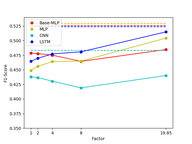
The results of our experiments are shown in Table 2. In addition, we plot the performance of each method as a function of the number of samples used for training the title model. These are shown in Figure 2.

Table 2. Results of experiments in terms of sample-based

F_{1}

-measure. The best performing method on each sub-dataset is printed in bold font.

	EconBiz $F_{1}$ scores						PubMed $F_{1}$ scores
	Full-Text	T1	T2	T4	T8	$T_{all}$	Full-Text	T1	T2	T4	T8	$T_{all}$
Base-MLP	0.441	0.391	0.419	0.442	0.451	0.472	0.526	0.479	0.478	0.475	0.465	0.485
MLP	0.457	0.357	0.396	0.432	0.453	0.500	0.530	0.449	0.456	0.464	0.465	0.504
CNN	0.387	0.364	0.382	0.400	0.407	0.426	0.483	0.438	0.437	0.431	0.419	0.440
LSTM	0.363	0.360	0.392	0.417	0.435	0.466	0.524	0.465	0.470	0.477	0.481	0.515

EconBiz

On the EconBiz dataset, the best results on both titles and full-texts are obtained by MLP. The title-based method is on par with the full-text method when eight times as many titles as full-texts are used. When all titles are used, the title-MLP outperforms its full-text counterpart by 9.4%, achieving an $F_{1}$ -score of 0.500. In contrast, when the same number of samples for full-text and titles is used, the gap between the best title method (Base-MLP) and the best full-text method (MLP) is 16.9% in favor of the full-text.

The MLP seems to benefit the most from additional titles. Initially, when as many titles as full-texts are used for training, all our proposed methods, i. e., MLP, CNN, and LSTM, perform within 0.007 points in $F_{1}$ -score from each other, but MLP performs worst. However, the relation flips as more titles are added. In Figure 2 (a), we can observe that MLP has the steepest curve of improvement out of all methods, in particular when considering the improvement from T1 to T2. With twice as many titles as full-texts, MLP is already the best performing classifier out of the ones we have proposed. The gap to the other methods only gets wider as more data is added for training. Overall, the MLPs performance on $T_{all}$ improves over the performance on T1 by 40.1%. The other methods also improve continuously as more training data is added. However, the CNN and LSTM improve by only 17% and 29.4% with respect to T1, respectively. Still, this is enough to surpass their full-texts counterparts by 10.1% and 28.4%, respectively.

When using as many titles as full-texts, Base-MLP outperforms our proposed methods clearly by 0.027 points in $F_{1}$ -score. However, Base-MLP does not benefit as much from additional training data. Its overall improvement is only 20.7%, so when all titles are used for training, it is outperformed by MLP by a margin of 5.9%. On the full-text, MLP has an advantage of 3.6% over the baseline. Yet, the baseline still has a large advantage over LSTM and CNN, both on titles and full-texts.

PubMed

On PubMed, MLP shows the best full-text performance, whereas LSTM yields the best results on titles. However, even when all titles are used for training, that is almost 20 times as many titles as full-texts, the LSTM still lacks behind the full-text MLP by 2.9%. However, this is a considerably smaller gap than when the same number of samples are used. Base-MLP, the best performing method on PubMed T1, achieves 10.7% lower scores than the best method on PubMed Full, which is MLP.

The MLP and the LSTM show very similar behavior when more training data is added. This can be seen from Figure 2 (b), where the lines of the MLP and LSTM are almost parallel. However, the overall improvement from T1 to $T_{all}$ is slightly higher for the MLP than for the LSTM. The former improves by 12.3%, whereas the latter improves by 10.8%. The CNN does not seem to benefit from additional data at all. Initially, on T1, the CNN performs relatively close to the other methods, lacking behind the LSTM by 5.7%. However, as more data is added for training, the CNN demonstrates a worse classification performance than with fewer training samples. Only when all available titles are used, the CNN barely outperforms itself on T1 by a very slim margin of 0.5%. Consequently, the CNN has the largest difference to its full-text counterpart out of all proposed methods. It scores 9.8% lower on $T_{all}$ than on PubMed Full, whereas the gap is 5.2% for the MLP and 1.8% for the LSTM.

By a considerable margin, the baseline is the best method on T1, where relatively few samples are used for training. However, despite using 20 times as many training samples, the performance on $T_{all}$ is only 1.3% better, which is a difference to the MLP and LSTM of 3.9% and 6.2%, respectively. As it is the case on the EconBiz dataset, the full-text performance of BaseMLP is the second best and gets as close to the MLP as 0.8%.

6. Discussion

The main question of our study is to which extent title-based methods can catch up to the performance of full-text-based methods by increasing the amount of title training data. On EconBiz, the best title-based method outperforms the best full-text method by 9.4% when all title training data is used. Considering that the difference is 16.9% in favor of the full-text when the sample sizes are equal, this is an impressive improvement. On PubMed, the improvement is less astounding. However, the title-based method is close to competitive to the full-texts, as the difference in score (less than 3%) is small. Considering that the gap is much larger for equal sample sizes (10.7%), we must acknowledge that current machine learning techniques in combination with large quantities of data are able to obtain just as good classification performance by merely using the titles.

However, in order to utilize title-based methods in a particular application, it is important to understand why there is such a large difference between the EconBiz and PubMed datasets regarding the benefit of employing title-based methods with large amounts of data. A possible explanation for that difference lies in the absolute numbers of full-texts available for training. As we have pointed out, previous literature suggests that deep learning models require around 650,000 samples to outperform more traditional approaches. On EconBiz, this number of full-texts is far from being reached. Due to this lack of enough training data, our deep learning models may not do so well with full-texts, in absolute numbers. The models based on titles on the other hand may be able to achieve their impressive results because there is just enough data to unleash the power of deep learning models. In fact, our MLP, which was optimized for large sample sizes, starts to outperform the baseline when eight times as many titles as full-texts are used, which nets to approximately 560,000 training samples. On the PubMed dataset, there are almost 650,000 full-text samples available. Here, the deep learning models can already work well on full-text. This may explain why the LSTM performs so much better on PubMed’s full-texts than on EconBiz’s full-texts. These findings support the claim from previous literature that deep learning models work well for text classification only when the sample size is several hundred thousands. Furthermore, since our datasets have large label spaces, we can state that this observation extents to XMLC, which is arguably a harder task than single-label classification.

In order to push the limits of text classification based on titles, our strategy was to develop and employ methods that can make use of the vast amount of data available for training. Our results suggest that this strategy was largely successful. On both datasets, some of our methods surpass the performance of the baseline as they are given more and more data for training. BaseMLP on the other hand cannot make such good use of the additional training data. This becomes particularly apparent on the PubMed dataset, where it improves by only 1.3% even when it has 20 times more training data. Our methods on the other hand improve considerably the more data is used for training. To be fair, it is clear that part of the much larger gain compared to the baseline is due to overfitting on the small title datasets such as T1. Recall that our methods are optimized towards their performance on $T_{all}$ . This design decision in our study was made to be able to fairly assess the development of the performance as the sample size increases. We observed that the capacity of the resulting models is likely too large for smaller datasets, which results in overfitting. This can be seen by the fact that BaseMLP, which has considerably lower capacity, outperforms our proposed methods on both PubMed and EconBiz. Yet, on $T_{all}$ , MLP outperforms Base-MLP by a wide margin on both datasets. LSTM is close to Base-MLP on EconBiz and outperforms it drastically on PubMed. Again, this indicates the success of our strategy. The only exception is the CNN, which does not benefit as much from additional data as our other proposed methods, although its capacity is large compared to other architectures recently proposed in the literature. It is particularly interesting that the performance of CNN (and Base-MLP, too) actually has a drop on PubMed as more title samples are used for training. We explain this by the fact that in T2 to T8 more than 1,300 new labels that do not occur in T1 are introduced. Hence, the models have to account for these new labels even though they never appear in the test set, reducing their capacity to learn to classify the labels relevant to the test set.

Considering the amount of attention CNNs have received in recent years for their performance in text classification (cf. Section 2), the results of our CNN is rather underwhelming. This is true for both full-text, and titles. In neither case is this due to overfitting. Our preliminary experiments showed that the CNN benefits from increasing the feature map size a lot. Yet, the CNNs do not benefit from additional training data in the same way LSTMs and MLPs do. On PubMed, no benefit at all can be observed. On EconBiz, the rate of improvement is comparable to MLP and LSTM only up to a factor of four times the number of full-texts. After that, the improvement is relatively marginal. In conclusion of our findings, we think it would be good if future research shifted its focus more towards MLPs and LSTMs, as they have demonstrated to be serious competitors for CNNs in text classification.

The goal of this study is to investigate to which extent a model trained on vast amounts of sample titles can compensate for the lack of information in comparison to the full-text. Thus, it is not the aim to achieve results beyond the state-of-the-art performance on, e. g., full-texts. Yet, the models we use are based on and also enhance recently proposed models. As described in Section 3.1, the MLP is at its core a non-linear version of the popular fastText. The CNN is based on recent advances from the domain of text-based XMLC, but was improved by integrating more fine-grained window sizes and larger feature maps. Finally, we present a strong bidirectional LSTM with attention over the outputs that does not assume a hierarchical structure of the document and therefore also works for short text snippets, in contrast to previous work by Yang et al. (Yang et al., 2016). Therefore, our methods are good candidates for researchers to also adopt for single-label text classification.

A common problem in machine learning research and in deep learning in particular is that models are very sensitive to the choice of hyperparameters. However, examining the whole hyperparameter space is very difficult due to its combinatorial complexity. Recently, this has called the validity of deep learning results into question, for example in language-modeling (Melis et al., 2017) or even text classification (Le et al., 2018). This problem persists in our study as well. However, instead of simply assuming values for our parameters or manually tuning them in a somewhat arbitrary fashion, we took an incremental tuning approach that in the end led to an improvement over initial base models from the literature in all cases. This gives us reason to believe that our results are largely reliable.

In this study, we have compared three deep learning methods. We did not compare against linear models such as logistic regression, and we did not compare against other non-linear approaches such as kNN or SVMs. However, as described in Section 2, there is evidence that traditional linear methods are inferior to non-linear ones when the training data is large. More importantly, we compared against a non-linear baseline by Galke et al. (Galke et al., 2017a) that was shown to outperform not only linear models, but also other non-linear, non-parametric models like kNN and SVMs on a diverse set of datasets and by a wide margin on both titles and full-texts.

For comparability, our proposed models were chosen such that they can be employed to titles and full-texts uniformly. This prohibits that certain strengts of the full-text can be made full use of. For instance, full-text models might benefit greatly from a hierarchical model as proposed by Yang et al. (Yang et al., 2016). On the other hand, we tried our best to tap the full potential of full-texts. For instance, in our CNN we employ dynamic max-pooling with $p=3$ for full-texts although this does not have any beneficial effect on titles.

In our study, we have examined two datasets from digital libraries of scientific content. We argue that these results are likely to generalize to other datasets of scientific publications as well. In consent with previous text classification research, we found our deep learning methods to require approximately 550,000 samples to outperform the previous baseline (EconBiz T8). While this number of titles can certainly be reached in domains other than economics and biomedicine, not many scientific domains will reach this number of full-texts. This can be seen by considering the fact that the availability of full-texts is generally tied to their open access rate. The rate of open access journals in academia is approximately 7% as reported by Teplitskiy et al. (Teplitskiy et al., 2017). This number closely matches the rate of 5 to 6.5% of available full-texts in our datasets. Moreover, Teplitskiy et al.’s study also suggests that the corpus of publications from the medical domain are among the largest. Therefore, we think it is likely that in other domains at least the relatively small gap of less than 3% between titles and full-texts can be achieved as well. However, in many other domains where only few full-texts are available, training models on titles may actually be much better, as we demonstrated for the economics domain.

Our results are of great practical importance for automatic semantic indexing in digital libraries. Considering the large amount of new literature published every year, subject indexers rely on the assistance of machines. It is desirable to have algorithms that produce good annotation suggestions by using only the title as textual input instead of the abstract or full-text. This is because the title is easy to obtain and free to use in text mining applications, whereas the full-text and even the abstract are often either not available or may not be processed automatically due to legal restrictions. For instance, in EconBiz only approximately 15% of the documents have an abstract and 7% have a full-text available. Furthermore, the task of downloading and processing the full-text is cumbersome, where one has tens of gigabytes of data. In contrast, as Table 1 shows, titles only comprise up to a few gigabytes of data. Thus, the full-text are by an order of magnitude larger. Thanks to the vast amount of data available for training title-based deep learning models, our study demonstrates that in a realistic scenario deep learning algorithms are able to satisfy the demand for sufficiently strong title-based classification methods. Engineers of (semi-)automatic semantic indexing algorithms should therefore consider shifting their focus from full-text-based classification to title-based classification in order to maximize the applicability of automatic semantic indexing systems.

7. Conclusion

In this paper, we have successfully answered the question if a semantic indexing system based on the title can reach the performance of a system based on the full-text if the number of samples for training the title-based method is much larger than the number of full-text samples. To this end, we developed three deep learning methods and evaluated them on two scientific datasets of different size. We found that in one case such a system is competitive with the full-text system, and in the other case it even yields considerably better scores. These results have important implications for automatic semantic indexing systems in digital libraries of scientific content.

In the future, we want to push the limits of classification based on large amounts of titles even further, and we would like to encourage the community to do the same. To this end, we published the title datasets, the source code, and an extended version of this paper on GitHub¹¹¹¹ 11 https://github.com/florianmai/Quadflor.

Acknowledgements.

This research was co-financed by the Sponsor EU H2020 project MOVING (http://www.moving-project.eu/) under contract no Grant #693092. We would like to thank Tamara Pianos and Tobias Rebholz from ZBW for providing helpful information on the EconBiz dataset.

References

Brain and Webb (1999) Damien Brain and G Webb. 1999. On the effect of data set size on bias and variance in classification learning. In Australian Knowledge Acquisition Workshop, AI’99. 117–128.
Conneau et al. (2017) Alexis Conneau, Holger Schwenk, Loïc Barrault, and Yann Lecun. 2017. Very deep convolutional networks for text classification. In ECACL, Vol. 1. 1107–1116.
Gal and Ghahramani (2016) Yarin Gal and Zoubin Ghahramani. 2016. A Theoretically Grounded Application of Dropout in Recurrent Neural Networks. In NIPS. 1019–1027.
Galke et al. (2017a) Lukas Galke, Florian Mai, Alan Schelten, Dennis Brunsch, and Ansgar Scherp. 2017a. Using Titles vs. Full-text as Source for Automated Semantic Document Annotation. In K-CAP. 9.
Galke et al. (2017b) Lukas Galke, Ahmed Saleh, and Ansgar Scherp. 2017b. Word Embeddings for Practical Information Retrieval. In INFORMATIK. 2155–2167.
Grave et al. (2017) Edouard Grave, Tomas Mikolov, Armand Joulin, and Piotr Bojanowski. 2017. Bag of Tricks for Efficient Text Classification. In EACL. 427–431.
Greff et al. (2017) Klaus Greff, Rupesh K Srivastava, Jan Koutník, Bas R Steunebrink, and Jürgen Schmidhuber. 2017. LSTM: A search space odyssey. IEEE TNNLS (2017).
Große-Bölting et al. (2015) Gregor Große-Bölting, Chifumi Nishioka, and Ansgar Scherp. 2015. A comparison of different strategies for automated semantic document annotation. In K-CAP. ACM, 8.
He et al. (2016) Kaiming He, Xiangyu Zhang, Shaoqing Ren, and Jian Sun. 2016. Deep residual learning for image recognition. In CVPR. 770–778.
Hemminger et al. (2007) Bradley M Hemminger, Billy Saelim, Patrick F Sullivan, and Todd J Vision. 2007. Comparison of full-text searching to metadata searching for genes in two biomedical literature cohorts. JASIST 58, 14 (2007), 2341–2352.
Hochreiter and Schmidhuber (1997) Sepp Hochreiter and Jürgen Schmidhuber. 1997. Long short-term memory. Neural computation 9, 8 (1997), 1735–1780.
Huang et al. (2011) Minlie Huang, Aurélie Névéol, and Zhiyong Lu. 2011. Recommending MeSH terms for annotating biomedical articles. JAMIA 18, 5 (2011), 660–667.
Ioffe and Szegedy (2015) Sergey Ioffe and Christian Szegedy. 2015. Batch Normalization: Accelerating Deep Network Training by Reducing Internal Covariate Shift. In ICML. 448–456.
Joachims (1998) Thorsten Joachims. 1998. Text Categorization with Support Vector Machines: Learning with Many Relevant Features. In ECML. Springer-Verlag, 137–142.
Kim (2014) Yoon Kim. 2014. Convolutional Neural Networks for Sentence Classification. In EMNLP. 1746–1751.
Kingma and Ba (2014) Diederik Kingma and Jimmy Ba. 2014. Adam: A method for stochastic optimization. arXiv:1412.6980 (2014).
Le et al. (2018) Hoa T Le, Christophe Cerisara, and Alexandre Denis. 2018. Do Convolutional Networks need to be Deep for Text Classification?. In Proceedings of the AAAI-18 Workshop on Affective Content Analysis, New Orleans, Louisiana, United States, February 3rd.
LeCun et al. (2015) Yann LeCun, Yoshua Bengio, and Geoffrey Hinton. 2015. Deep learning. Nature 521, 7553 (2015), 436–444.
Liu et al. (2017) Jingzhou Liu, Wei-Cheng Chang, Yuexin Wu, and Yiming Yang. 2017. Deep Learning for Extreme Multi-label Text Classification. In SIGIR. ACM, 115–124.
Liu et al. (2015) Ke Liu, Shengwen Peng, Junqiu Wu, Chengxiang Zhai, Hiroshi Mamitsuka, and Shanfeng Zhu. 2015. MeSHLabeler: improving the accuracy of large-scale MeSH indexing by integrating diverse evidence. Bioinformatics 31, 12 (2015), i339–i347.
Mao and Lu (2017) Yuqing Mao and Zhiyong Lu. 2017. MeSH Now: automatic MeSH indexing at PubMed scale via learning to rank. J. of Biomedical Semantics 8, 1 (2017), 15.
Melis et al. (2017) Gábor Melis, Chris Dyer, and Phil Blunsom. 2017. On the state of the art of evaluation in neural language models. arXiv:1707.05589 (2017).
Mork et al. (2014) James G Mork, Dina Demner-Fushman, Susan Schmidt, and Alan R Aronson. 2014. Recent Enhancements to the NLM Medical Text Indexer.. In Working Notes for CLEF. 1328–1336.
Nam et al. (2014) Jinseok Nam, Jungi Kim, Eneldo Loza Mencía, Iryna Gurevych, and Johannes Fürnkranz. 2014. Large-Scale Multi-label Text Classification - Revisiting Neural Networks. In ECML. 437–452.
Nascimento et al. (2011) Cristiano Nascimento, Alberto HF Laender, Altigran S da Silva, and Marcos André Gonçalves. 2011. A source independent framework for research paper recommendation. In JCDL. ACM, 297–306.
Nishioka and Scherp (2016) Chifumi Nishioka and Ansgar Scherp. 2016. Profiling vs. Time vs. Content: What does Matter for Top-k Publication Recommendation based on Twitter Profiles?. In JCDL. ACM, 171–180.
Pennington et al. (2014) Jeffrey Pennington, Richard Socher, and Christopher D. Manning. 2014. Glove: Global Vectors for Word Representation. In EMNLP. 1532–1543.
Rubin et al. (2012) Timothy N Rubin, America Chambers, Padhraic Smyth, and Mark Steyvers. 2012. Statistical topic models for multi-label document classification. JMLR 88, 1 (2012), 157–208.
Salton and Buckley (1988) Gerard Salton and Christopher Buckley. 1988. Term-weighting approaches in automatic text retrieval. Information processing & management 24, 5 (1988), 513–523.
Srivastava et al. (2014) Nitish Srivastava, Geoffrey E Hinton, Alex Krizhevsky, Ilya Sutskever, and Ruslan Salakhutdinov. 2014. Dropout: a simple way to prevent neural networks from overfitting. JMLR 15, 1 (2014), 1929–1958.
Tai et al. (2015) Kai Sheng Tai, Richard Socher, and Christopher D. Manning. 2015. Improved Semantic Representations From Tree-Structured Long Short-Term Memory Networks. In ACL. 1556–1566.
Teplitskiy et al. (2017) Misha Teplitskiy, Grace Lu, and Eamon Duede. 2017. Amplifying the impact of open access: Wikipedia and the diffusion of science. JASIST 68, 9 (2017), 2116–2127.
Tsatsaronis et al. (2015) George Tsatsaronis, Georgios Balikas, Prodromos Malakasiotis, Ioannis Partalas, Matthias Zschunke, Michael R Alvers, Dirk Weissenborn, Anastasia Krithara, Sergios Petridis, Dimitris Polychronopoulos, Yannis Almirantis, John Pavlopoulos, Nicolas Baskiotis, Patrick Gallinari, Thierry Artieres, Axel Ngonga, Norman Heino, Eric Gaussier, Liliana Barrio-Alvers, Michael Schroeder, Ion Androutsopoulos, and Georgios Paliouras. 2015. An overview of the BIOASQ large-scale biomedical semantic indexing and question answering competition. BMC Bioinformatics 16 (2015), 138.
Xiao and Cho (2016) Yijun Xiao and Kyunghyun Cho. 2016. Efficient character-level document classification by combining convolution and recurrent layers. arXiv:1602.00367 (2016).
Yang et al. (2016) Zichao Yang, Diyi Yang, Chris Dyer, Xiaodong He, Alexander J. Smola, and Eduard H. Hovy. 2016. Hierarchical Attention Networks for Document Classification. In NAACL-HLT. 1480–1489.
Yin et al. (2017) Wenpeng Yin, Katharina Kann, Mo Yu, and Hinrich Schütze. 2017. Comparative Study of CNN and RNN for Natural Language Processing. arXiv:1702.01923 (2017).
Yin and Schütze (2015) Wenpeng Yin and Hinrich Schütze. 2015. Multichannel Variable-Size Convolution for Sentence Classification. In CoNLL. 204–214.
Yogatama et al. (2017) Dani Yogatama, Chris Dyer, Wang Ling, and Phil Blunsom. 2017. Generative and discriminative text classification with recurrent neural networks. arXiv:1703.01898 (2017).
Young et al. (2017) Tom Young, Devamanyu Hazarika, Soujanya Poria, and Erik Cambria. 2017. Recent trends in deep learning based natural language processing. arXiv:1708.02709 (2017).
Zhang and Zhou (2006) Min-Ling Zhang and Zhi-Hua Zhou. 2006. Multilabel neural networks with applications to functional genomics and text categorization. IEEE TKDE 18, 10 (2006), 1338–1351.
Zhang et al. (2016) Rui Zhang, Honglak Lee, and Dragomir R. Radev. 2016. Dependency Sensitive Convolutional Neural Networks for Modeling Sentences and Documents. In NAACL-HLT. 1512–1521.
Zhang et al. (2017) Wenjie Zhang, Liwei Wang, Junchi Yan, Xiangfeng Wang, and Hongyuan Zha. 2017. Deep Extreme Multi-label Learning. arXiv:1704.03718 (2017).
Zhang et al. (2015) Xiang Zhang, Junbo Zhao, and Yann LeCun. 2015. Character-level convolutional networks for text classification. In NIPS. 649–657.