Secrecy Capacity of Colored Gaussian Noise Channels with Feedback
Abstract
In this paper, the -th order autoregressive moving average (ARMA(k)) Gaussian wiretap channel with noiseless causal feedback is considered, in which an eavesdropper receives noisy observations of the signals in both forward and feedback channels. It is shown that a variant of the generalized Schalkwijk-Kailath scheme, a capacity-achieving coding scheme for the feedback Gaussian channel, achieves the same maximum rate for the same channel with the presence of an eavesdropper. Therefore, the secrecy capacity is equal to the feedback capacity without the presence of an eavesdropper for the feedback channel. Furthermore, the results are extended to the additive white Gaussian noise (AWGN) channel with quantized feedback. It is shown that the proposed coding scheme achieves a positive secrecy rate. As the amplitude of the quantization noise decreases to zero, the secrecy rate converges to the capacity of the AWGN channel.
Index Terms:
Secrecy Capacity, Feedback, Colored Gaussian, Schalkwijk-Kailath SchemeI Introduction
It has been more than a half century since the information theorists started to investigate the capacity of feedback Gaussian channels. As the pioneering studies on this topic, Shannon’s 1956 paper [2] showed that feedback does not increase the capacity of the memoryless AWGN channel, and Elias [3] [4] proposed some simple corresponding feedback coding schemes. Schalkwijk and Kailath [5] [6] then developed a notable linear feedback coding scheme to achieve the capacity of the feedback AWGN channel. Thereafter, the problem of finding the feedback capacity and the capacity-achieving codes for the memory Gaussian channels (e.g. ARMA(k)) has been extensively studied. Butman [7] [8], Wolfowitz [9] and Ozarow [10] [11] extended Schalkwijk’s scheme to ARMA(k) Gaussian channels, leading to several valuable upper and lower bounds on the capacity. Motivated by these elegant results/insights, in Cover and Pombra [12] made a breakthrough on characterizing the -block capacity of the feedback Gaussian channel. In , Kim [13] provided a characterization (in the form of an infinite dimensional optimization problem) of the capacity of the ARMA(k) feedback Gaussian channel based on Cover-Pombra’s -block capacity characterization. Unfortunately, except for the first-order ARMA noise, it is non-trivial to compute the capacity by solving this infinite dimensional optimization. Recently, Gattami [14] showed that the capacity of the stationary Gaussian noise channel with finite memory can be found by solving a semi-definite programming problem. In addition, Li and Elia [15] [16] utilized the control-theoretic tools to compute the capacity of the ARMA(k) feedback Gaussian channel and construct the capacity-achieving feedback codes.
As a natural extension of the above results, the ARMA(k) feedback Gaussian channel with an eavesdropper that has noisy access of channel transmissions is of much interest. Concretely, two fundamental questions can be asked: 1). would the feedback capacity of such a channel decrease subject to the secrecy constraint? 2). what would be the secrecy capacity-achieving codes? In fact, secure communications over feedback channels have attracted a lot of attention over the last decade. Substantial progresses have been made towards understanding this type of channels. In particular, although the feedback may not increase the capacity of open-loop AWGN channels, [17, 18, 19, 20, 21, 22, 23, 24, 25, 26] showed that feedback can increase the secrecy capacity by sharing a secret key between legitimate users or roiling the codewords from eavesdroppers’ observations. For instance, [17] and [18] showed the achievement of a positive secrecy rate by using noiseless feedback even when the secrecy capacity of the feed-forward channel is zero. Furthermore, [27] presented an achievable scheme for the wiretap channel with generalized feedback, which is a generalization and unification of several relevant previous results in the literature. Very recently, [28] proposed an improved feedback coding scheme for the wiretap channel with noiseless feedback, which was shown to outperform the existing ones in the literature.
On the other hand, the multiple-access (MA) wiretap channel with feedback has also been studied in recent a few years. [29] derived achievable secrecy rate regions for discrete memoryless Gaussian channels where two trusted users send independent confidential messages to an intended receiver in the presence of a passive eavesdropper. [30] developed inner and outer bounds on the secrecy rate region for the MA wiretap channel with noiseless feedback. In a more general setting where users have multiple-input multiple-output (MIMO) equipments, [31] characterized the pre-log factor of the secrecy rate in the case with the number of antennas at the source being no larger than that at the eavesdropper. [32] and [33] investigated the benefits of state-feedback to increase the secrecy degrees of freedom for the two-user Gaussian MIMO wiretap channel.
However, it is noteworthy that most of the aforementioned results on both the point-to-point and the MA communications only considered memoryless wiretap channels. Thus motivated, in this paper we consider a memory wiretap channel (i.e. ARMA(k) Gaussian noise channel) with feedback and make two major contributions.
- 1.
We propose a variant of the generalized - scheme, which achieves the feedback capacity of the ARMA(k) Gaussian noise channel without an eavesdropper and show that the proposed coding scheme also achieves the same maximum rate of such a channel with an eavesdropper.
- 2.
We further study the AWGN channel with quantized feedback, which is a more realistic channel model for the feedback link. We show that the proposed coding scheme provides non-trivial positive secrecy rates and achieves the feedback capacity of the AWGN channel as the amplitude of the quantization noise vanishes to zero.
The rest of the paper is organized as follows. In Section II and III, we introduce the system model and the preliminary results, respectively. Section IV presents the main results of our paper. Section V provides the technical proofs. Finally, in Section VI, we conclude the paper and outline possible research venues down the road.
Notation: Uppercase and the corresponding lowercase letters denote random variables and their realizations, respectively. We use to denote the logarithm with base , and . We use to denote the transpose of a vector or matrix . The symbol denotes the set of bounded continuous functions on . denotes the set of stable and proper rational filters in Hardy space , and denotes the 2-norm Lebesgue space.
II System Model
In this section, we present the mathematical system model. First of all, we consider a discrete-time Gaussian channel with noiseless feedback (Fig. 1). The additive Gaussian channel is modeled as
| (1) |
where the Gaussian noise is assumed to be stationary with power spectrum density for . Unless the contrary is explicitly stated, “stationary” without specification refers to stationary in wide sense. Moreover, we assume the power spectral density satisfies the Paley-Wiener condition

Assumption 1.
(ARMA(k) Gaussian Channel) In this paper, noise is assumed as the output of a finite-dimensional linear time invariance (LTI) minimum-phase stable system , driven by the white Gaussian noise with zero mean and unit variance. The power spectral density (PSD) of is colored (nonwhite)11 1 Both the (Shannon) capacity [2] and the secrecy capacity [23] for the AWGN channel with noiseless causal feedback have been known., bounded away from zero and has a canonical spectral factorization given by .
As shown in Fig.1, the feedback wiretap channel of interest includes a forward channel from Alice to Bob as described by (1), a causal noiseless feedback from Bob to Alice, and three noisy observation channels to the eavesdropper Eve. Note that a classical wiretap channel model can be recovered if the eavesdropper’s channel input and are removed. In this paper, we assume that the eavesdropper is powerful and can access three inputs 22 2 Note that in [1] only the access to channel input and channel output is considered. Based on the generalized results in this paper, however, the results in [1] with three noisy observation channels to the eavesdropper as assumed in this paper still hold.. The noisy wiretap channels are modeled as
The additive noises , and are assumed to be arbitrarily finite-memory channels, i.e.,
| (2) |
where , and respectively represent the size of finite memories and the notation represents a sequence in a compact form. In this paper, we assume these noises have strictly positive and bounded variance for all . But they are not necessarily uncorrelated.
We specify a sequence of channel codes with an achievable secrecy rate as follows. We denote the message index by , which is uniformly distributed over the set . The encoding process at Alice satisfies the average transmit power constraint , where () for and . Bob decodes the message to be by following a decoding function : with an error probability satisfying , where . Meanwhile, the information received by Eve should asymptotically vanish, i.e., . The objective of secure communications is to send to Bob at an as high rate as possible. The secrecy capacity is defined as the supremium of all achievable rates . Mathematically,
| (3) |
where the “feasible coding schemes” refer to all feedback codes satisfying the secrecy requirements and the power constraint. Note that the feedback capacity (without the secrecy constraint) from Alice to Bob, denoted as , can be recovered by removing the secrecy constraint. This implies .
III Preliminaries of feedback capacity and capacity-achieving coding scheme
In this section, we review the characterization of the feedback capacity and then propose a variant of the generalized - scheme, which is a -achieving feedback codes without the presence of an eavesdropper. The materials here are useful for us to further investigate the channel model with an eavesdropper.
III-A Feedback Capacity Revisited
Firstly, we present the feedback capacity characterization for the Gaussian channel under Assumption 1. As proved in [13], the feedback capacity from Alice to Bob for such a channel with the average power budget can be characterized by
| (4) |
Remark 1.
When specified to ARMA(1) channel, the above characterization can be simplified and has a closed-form solution.
Lemma 1.
(Theorem 5.3 in [13]) For the ARMA(1) feedback Gaussian channel with the average channel input power budget , the feedback capacity is given by
where is the unique positive root of the fourth-order polynomial in
and
Furthermore, an optimal to achieve is given by
| (5) |
Since the optimization in (4) has infinite dimensional search space, except for the ARMA(1) Gaussian channels, neither the analytical nor the numerical solutions to was known in the literature. One recent result in [14] casted the above optimization into a semi-definite programming and then used the convex tools to compute . In addition, [15] [16] provided a numerical approach to compute and explicitly construct the optimal , which can be efficiently solved by the standard convex optimization tools. We refer the interested reader to [15] [16] for details. To make our paper self-contained, we re-state the main results in [15] [16] as follows.
Proposition 1.
Remark 2.
With a bit abuse of notation, we use instead of for simplicity. The basic idea to obtain the characterization (6) is that the strict causality constraint (4) can be equivalently imposed on (the infinite number of) the non-positive index coefficients of the inverse Fourier transform of by setting them to zeros. The upper bound follows as we herein only impose a finite number of the Fourier coefficients with non-positive index to be zero.
Notice that still turns out to be a semi-infinite dimensional problem, in which there are finite number of constraints but infinite number of feasible solutions in . However, one important result, as shown below, establishes the strong Lagrangian dual of . In other words, there is no duality gap between the semi-infinite dimensional primal problem and its finite dimensional dual problem, a fact that provides a convex optimization approach to compute .
Theorem 1.
(Theorem 2 in [15]) Under Assumption 1, let
For , , and , define
Then, the following statements hold.
a) The Lagrangian dual of (6) is given by
| (8) |
where
| (9) |
with
| (10) |
b) The dual problem (D) in (8) is equivalent to the following convex optimization problem
| (11) |
where
| (12) |
and the optimal is characterized by (10).
c) Furthermore, , and an optimal strictly casual filter for exists and is characterized by
| (13) |
Note that the above optimization is not easily computable due to the integral in the objective function. A natural approach is to approximate the integral with a finite sum by discretizing . We apply such discretization to (11) (with spacing ) and introduce the following finite dimensional convex problem. Given , consider
| (14) |
where
and .
It is argued in [16] that can be an arbitrarily well approximation of , i.e., .
Notice that the optimization (14) is in a simple convex form. In particular, the of an affine function is concave. The term is quadratic (composed with an affine function of the variables) over linear function, therefore convex. Thus, (14) can be efficiently solved with the standard convex optimization tools, e.g. CVX, a package for specifying and solving convex programs[34, 35].
In what follows, we describe, given an optimal in (4), how to construct an implementable coding scheme that achieves the feedback capacity from Alice to Bob.

III-B -achieving Feedback Coding Scheme
First of all, once an optimal is found for the above optimization, we construct a feedback filter stabilizing the channel within the prescribed input average power budget (see [15] for proofs). Next, based on the transfer function , we construct an explicit feedback coding scheme as follows, which is deterministic (time-invariant) and has doubly exponential decaying decoding error probability.
We first present controller as a LTI single-input-single-output (SISO) finite-dimensional discrete-time unstable system with the following state-space model:
| (15) |
Based on Remark 1, we assume that the eigenvalues of are strictly outside the unit disc while the eigenvalues of are strictly inside the unit disc. Without loss of generality, we assume that and are in Jordan form. Assume has eigenvalues, denoted by . Next, we review the coding scheme in [16] [36] (Fig. 2), which decompose into an encoder (Alice) and a decoder (Bob) with an estimated signal fed back to the encoder via the noiseless feedback channel.
Decoder: The decoder runs driven by the channel output .
It produces two signals: an estimate of the initial condition of the encoder
and a feedback signal
Encoder: The encoder runs the following dynamics
It receives and produces the channel input
As will be seen later, the above coding scheme cannot be directly applied to the feedback ARMA(k) Gaussian channel with an eavesdropper. Therefore, we next propose an equivalent representation of the above decoder-estimation-based feedback coding scheme. It will be proved that a variant of this new representation achieves the same maximum rate of the same channel without the eavesdropper.
Representation II: Channel-output-based Feedback Coding Scheme (Fig. 3).
Decoder: The decoder runs driven by the channel output .
It only produces an estimate of the initial condition of the encoder
Encoder: The encoder runs the following dynamics driven by the initial state, i.e., the message,
It receives and runs dynamics driven by the received feedback ,
and produces a signal
Then, the encoder produces the channel input

By comparing the two representations, we see that the only difference comes from the feedback signal. In Representation I, the feedback signal is generated by the decoder, while in Representation II, the feedback signal is simply the raw channel output. The equivalence can be directly verified by comparing the channel inputs (encoder) and the estimate of the message (decoder) of the two representations.
Proposition 2.
For a given message and a sequence of additive noise (), the Representation I and Representation II of the proposed coding scheme produce identical channel input and message estimate for .
Remark 3.
It is important to notice that the “equivalence” only holds for such a channel without an eavesdropper. This is because in our model the eavesdropper can access the feedback link. In Representation II, since the channel output is directly fed back to Alice, the eavesdropper’s access to both the channel output and the feedback link has no difference from the access to the channel output only. However, this is clearly not true for Representation I, in which the eavesdropper can extract more useful information from the decoding process (Bob) by accessing the feedback link.
We next provide some insight on the proposed coding scheme. All the discussions in the rest of this section hold for both representations.
First of all, in the above proposed coding schemes, since the closed loop is stable, goes to zero with time if the noise is not present. Given that
| (16) |
and the system is observable, we have . Thus, is an estimate at time of . In the presence of noise, Theorem 4.3 in [36] shows that the above coding scheme leads to for large , where represents the state covariance matrix. Note that, since the stable closed-loop system is observable and controllable, the matrix is positive definite (which converges to a steady state value and is independent from the initial state of the system) and so is . Since the eigenvalues of are strictly outside the unit disc, it is straightforward to see that the state covariance matrix converges to zero (e.g. element-wise) as goes to infinity.
In addition, in the above coding scheme the message index is allocated at the centroid of an unit hypercube in the coordinate system depending on . We refer interested readers to Theorem 4.3 in [36] for details. For scalar , the unit hypercube becomes an interval, e.g. . That is, messages are represented by the middle points of equally divided subintervals within . In the end, we note that the causality of the feedback channel is captured by the one-step delay of the state transition on and .
The next lemma indicates that the proposed coding scheme is -achieving. The proof is omitted as it follows directly from Theorem 4.3 and Theorem 4.6 in [36].
Proposition 3.
Consider stationary Gaussian channels in (4). Given a filter , the proposed coding scheme based on the decomposition of achieves a reliable transmission rate (in the sense of Shannon) at
and has double exponential decaying error probability.
This proposition indicates that the achievable rate of the proposed coding schemes (Representation I and Representation II) is explicitly characterized by the objective function in (4), leading to the fact that the proposed coding schemes are capacity-achieving if is an optimal solution to (4). Moreover, this achievable rate is only determined by the unstable eigenvalues of the system, implying that the capacity-achieving coding scheme must be unstable although the closed-loop system is stable.
Thus far, we have presented explicit feedback codes (in the state-space representation) that can achieve the feedback capacity. In the next section, we show that a variant of this coding scheme can lead to the asymptotic zero leakage of the message to Eve. This implies .
IV Main Results
In this section, we first present our results for the ARMA(k) feedback channel with an eavesdropper, and then extend our results to the case with quantization noise in feedback.
IV-A ARMA(k) Feedback Channel with an Eavesdropper
We first present our new development on the properties of the feedback coding scheme for ARMA(k) Gaussian channels without the presence of an eavesdropper. We then use these properties to establish our main theorem that characterizes the feedback secrecy capacity and its achieving coding scheme.
The following result shows that, by choosing the particular -step initializations (in the state-space representation) for the proposed coding scheme, the channel inputs () are only determined by the past additive Gaussian noise , a fact that is vital to guarantee the asymptotic secrecy from Eve.
Proposition 4.
For the proposed coding scheme in Fig. 2 or Fig. 3, assume the first -step channel inputs (where refers to matrix with power ), the estimate message (or equivalently, ) and , where is the number of the eigenvalues of matrix . Then the induced channel inputs for are only determined by the past Gaussian noise .
Proof.
See Section V-A. ∎
Proposition 5.
Proof.
The proof follows directly from two facts. On the one hand, all these initials have no effect on the average transmission power on channel inputs, which only depend on the steady state of the underlying LTI systems. On the other hand, these initials do not change the reliable transmission rate of the coding scheme , which is defined in an asymptotic manner and only determined by the unstable eigenvalues in (Proposition 3). ∎
This result provides a variant of the coding scheme , in which the first steps () of the channel input are different from others () and the states and of the coding dynamics are particularly initialized at . By doing so, after the initialization phase (), Alice only transmits the statistical learning information of “noise” rather than the message for in the forward channel, such that if only having access to the forward channel (which is essentially the case for Representation II) Eve cannot learn innovative information of the message through its noisy wiretap channels except in the first -steps.
Theorem 2.
Consider the ARMA(k) Gaussian wiretap channel with feedback (Fig. 1) under the average channel input power constraint . Then,
- 1.
the feedback secrecy capacity equals the feedback (Shannon) capacity, i.e., , where is obtained from Section III-A;
- 2.
the feedback secrecy capacity is achieved by the -achieving feedback coding scheme ( Representation II) with , (or equivalently, ), and .
Proof.
See Section V-B. ∎
This theorem shows that there exists a feedback coding scheme such that the secrecy requirement can be achieved without loss of the communication rate of the legitimate users. In addition, Section III-B provides such a feedback coding scheme that achieves the feedback secrecy capacity. In particular, a -achieving feedback code can be constructed from the optimal in (4) by following the procedures in Section III-B (Representation II) with the initializations defined in Proposition 4. The next corollary shows that the well-known - scheme [6] is a special case of our proposed coding scheme.
Corollary 1.
Consider the AWGN wiretap channel with feedback (Fig. 1) under the average channel input power constraint . Assume that the additive noise has zero mean and variance . Then the proposed coding scheme (Representation II) with and becomes the original S-K scheme, and achieves the secrecy capacity
Proof.
See Section V-C. ∎
This corollary recovers Theorem 5.1 in [23], showing that the well-known S-K scheme not only achieves the feedback capacity but also automatically provides the secrecy from the eavesdropper.
Remark 4.
As discussed in Remark 3, if the eavesdropper has no access to the feedback link, then the above results hold for the coding scheme in Representation I as well. That is, the feedback secrecy capacity is achieved by the -achieving feedback coding scheme (Representation I) with the selected initializations. The proof of this argument follows directly from the proof of Theorem 2 by deleting the eavesdropper’s access to the feedback link. Therefore, we conclude that the channel-output-based feedback coding scheme Representation II is highly necessary to remove the advantage of the eavesdropper’s access to the feedback link. If no such access, the “equivalence” between Representation I and Representation II holds for channels with the eavesdropper.
IV-B Feedback with Quantization Noise
In this section, we extend our result to Gaussian channels with quantized feedback. It is noteworthy that the capacity of colored Gaussian channels with noisy feedback remains an open problem [37] [38] [39], even when simplified to the quantization feedback. Therefore, in this paper, as an initial step towards the secrecy capacity of noisy feedback Gaussian channels, we focus on AWGN channels with quantized feedback. In [40], the authors presented a linear coding scheme featuring a positive information rate and a positive error exponent for AWGN channels with feedback corrupted by quantization or bounded noise. In what follows, we show that our proposed linear coding scheme Representation II, when specified to the AWGN channel with quantized feedback, converges to the scheme in [40] and, more importantly, leads to a positive secrecy rate. Furthermore, this achievable secrecy rate converges to the capacity of the AWGN channel as the amplitude of the quantization noise decreases to zero.
Firstly, we define a memoryless uniform quantizer with sensitivity as follows [40].
Definition 1.
Given a real parameter , a uniform quantizer with sensitivity is a function : defined as
where represents the floor function. Then, the quantization error at instant , i.e., the feedback noise, is given by
Notice that, for a given channel output , the quantization noise can be recovered by the decoder as we assume the decoder knows the quantization rule. In other words, the decoder can get access to both the channel outputs and the feedback noise while the encoder can only get access to the corrupted channel output. On the other hand, note that with the quantized feedback the coding schemes Representation I and Representation II are not equivalent any more due to the different feedback signals. The Representation I may not be applicable here. Therefore, we tailor the coding scheme Representation II to the AWGN channel with quantized feedback as follows (Fig. 4). We first let .
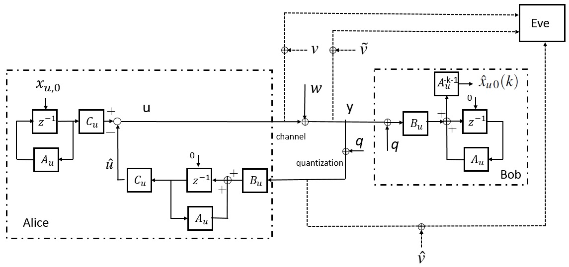
Decoder: The decoder runs driven by the sum of the channel output and the quantization noise .
It produces an estimate of the initial condition of the encoder
Encoder: The encoder runs the following dynamics
It receives and duplicates the decoding dynamics,
and produces a signal,
Then, it produces the channel input
We next show that the above coding scheme can achieve a positive secrecy rate, which converges to the AWGN capacity as the feedback noise decreases. The following definition will be used to characterize this secrecy rate.
Definition 2.
[40] For the given positive real parameters and the power constraint , define a parameter as follows.
- 1.
If , is the nonnegative real solution of the following equation,
- 2.
If , then .
It is easy to check that satisfies the following three properties [40]
- 1.
converges to the AWGN capacity as decreases, i.e.,
- 2.
If , we have .
- 3.
If , . In other words, the ratio of and converges to as .
Theorem 3.
Consider an AWGN channel with uniformly memoryless quantized feedback defined in Definition 1, where the channel input power constraint is and the noise variance of the AWGN channel and the quantization sensitivity in the feedback link are assumed to be and , respectively. Assume , and (or equivalently, ). Then, the above proposed coding scheme with and achieves a secrecy rate for all ( is defined in Definition 2).
Proof.
See Section V-D. ∎
Combined with the aforementioned property (1) on , this theorem implies that the achievable feedback secrecy rate of the proposed coding scheme converges to the AWGN capacity as decreases to zero.
V Technical Proofs
In this section, we present the omitted proofs in Sections IV.
V-A Proof of Proposition 4
Based on the Representation I of the proposed feedback coding scheme, we have
| (17) |
Next, for where the initial steps have passed and the signals evolve as described in the coding scheme, it yields
| (18) |
where step (a) follows from (17). Let and . Moving to the left side, we have
By iterating the above equation, for , we obtain
where we assume . Given and , we have
Then, it yields
Furthermore, given , from (17) we have
| (19) |
Now, for , we present the channel inputs and recall the evolution of as follows,
| (20) |
Starting with and , the above coupled iterations induce values of and that depend only on noise . Therefore, for
| (21) |
where the mapping is defined by the iterations in (20). Combining with (19), we conclude that, for , only depends on . Due to the equivalence between Representation I and Representation II of the coding scheme, this result directly holds for Representation II.
V-B Proof of Theorem 2
Following from Proposition 3, the proposed coding scheme derived from the optimal filter can achieve the feedback capacity . Then, in what follows, we only need to show that under the selected initializations of the proposed coding scheme, the following secrecy requirement is satisfied,
In this proof, we use the Representation II of the proposed coding scheme. Following from the model in Fig. 1 and (19), (21) in the proof of Proposition 4, the three inputs , and to Eve for are given by
| (22) |
and
| (23) |
and
| (24) |
where is the selected initializations. Recall that noises , and are additive noises defined in (2).
Then, for and we have
| (25) |
where follows from the fact that conditioning does not increase entropy, step follows from Proposition 4, step follows from (22), (23) and (24), step (d) follows from the finite memory of wiretap channel noise (, ,) and the last step follows from the fact that the noise is assumed to be independent from others.
Then, we obtain
| (26) |
where ( is an zero matrix) and . Recall that message is uniformly selected from that are equally spaced in an -dimensional unit hypercube. The covariance matrix of is as . Following from the fact that for a fixed covariance a vector Gaussian input distribution maximizes the mutual information, we obtain the following upper bound,
| (27) |
The last step follows from the fact that the right-hand side upper bound is independent from index . The proof is complete.
V-C Proof of Corollary 1
Based on the Schalkwijk’s scheme in [6], the channel input (encoder) and the message estimate (decoder) for are given below by using the notations in this paper.
| (28) |
The dynamics of the Schalkwijk’s coding scheme for can be summarized as follows,
| (29) |
where and is the variance of the additive white Gaussian noise in the forward channel.
In our coding scheme, for ,
| (30) |
Plugging these selected parameters into (17) and (18), we have channel inputs and the message estimate of our proposed coding scheme as follows,
| (31) |
By scaling the message and the corresponding estimate by factor , we recover the dynamics of the Schalkwijk’s scheme. Note that this constant scaling on the message index have no effect on the reliable transmission rate and the power cost at channel input. The proof is complete.
V-D Proof of Theorem 3
Starting from the decoder with and , we have the decoding dynamics ()
| (32) |
Then, the estimate of the initial state of the encoder (i.e., the message index) is
| (33) |
Next, based on (17) with and , we have the dynamics of channel inputs as
| (34) |
where step (a) follows from the above first two steps. Notice that our coding schemes of the decoder (33) and the encoder (34) are identical to the coding schemes (2) and (4) in [40]. In addition, Theorem 3.2 in [40] shows that, for a given (Definition 2), the proposed scheme can achieve any transmission rate with .
Now, we need to prove that the proposed coding scheme achieves secrecy with regard to the eavesdropper. In fact, we can directly follow the proof of Proposition 4 and characterize the channel inputs as
| (35) |
As a consequence, we note that the channel inputs of the proposed coding scheme only depend on the past forward channel noise and feedback quantization noise . This fact enables us to show that, by following the proof of Theorem 2, this coding scheme satisfies the secrecy requirement
To avoid redundancy, we herein only provide sketchy arguments. Details can be directly obtained by following (25) to (27).
| (36) |
Then, we obtain
| (37) |
where ( is an zero matrix) and . The rest of the proof is omitted as it directly follows from (27).
VI Conclusion
In this paper, we considered the ARMA(k) Gaussian wiretap channel with feedback and showed that a variant of the generalized - scheme, which is a feedback capacity-achieving code, secures transmissions by itself from the eavesdropper. Namely, the feedback secrecy capacity equals the feedback capacity without the presence of an eavesdropper. We further extended our scheme to the AWGN channel with quantized feedback and proved that our scheme can achieve a positive secrecy rate, which converges to the AWGN channel capacity as the quantization noise decreases to zero.
We conclude this paper by listing a few related research topics, which can facilitate to illustrate the complete picture of the secrecy communications with feedback. First of all, it is known that the - coding scheme nicely unifies communications, control and estimation for feedback systems. In this paper, by leveraging the tools from both control and communications, we showd that (a variant of) the - scheme automatically provides secrecy for the legitimate users. Therefore, understanding the secrecy nature of the - scheme from an estimation perspective could be a missing piece of the work. One possible investigation along this line is to extend the fundamental relation between the derivative of the mutual information and the MMSE [41], known as I-MMSE, from the open-loop channels to the feedback channels by invoking the direct information [42, 43] rather than the mutual information [44]. Furthermore, extend the current results to channels with noisy feedback can be very valuable. Toward this end, it is necessary to construct a feedback coding scheme with a good achievable rate for noisy feedback channels with no eavesdropper, which itself is a quite nontrivial problem in general. Finally, extensions to the multi-access colored Gaussian channels with feedback can be of much interest to the community in the field of secrecy communications.
References
- [1] C. Li and Y. Liang, “Secrecy capacity of the first-order autoregressive moving average gaussian channel with feedback,” in Proc. IEEE International Symposium on Information Theory, pp. 1963–1967, 2017.
- [2] C. Shannon, “The zero error capacity of a noisy channel,” Inst.Radio Eng. Trans.Information Theory, vol. IT-2, pp. S8–S19, 1956.
- [3] P. Elias, “Channel capacity without coding,” MIT Research Lab. of Electronics, Cambridge, MA, Quarterly Progr. Rep., 1956.
- [4] ——, “Networks of Gaussian channels with applications to feedback systems,” IEEE Trans. Inf. Theory, vol. 13, pp. 493 – 501, 1967.
- [5] J. P. M. Schalkwijk and T. Kailath, “A coding scheme for additive noise channels with feedback i: No bandwidth constraint,” IEEE Trans. Inf. Theory, vol. IT-12, no. 2, pp. 172–182, 1966.
- [6] J. P. M. Schalkwijk, “A coding scheme for additive noise channels with feedback ii: Band-limited signals,” IEEE Trans. Inf. Theory, vol. IT-12, no. 2, pp. 183–189, 1966.
- [7] S. Butman, “A general formulation of linear feedback communication systems with solutions,” IEEE Trans. Inf. Theory, vol. 15, no. 3, pp. 392 – 400, 1969.
- [8] ——, “Linear feedback rate bounds for regressive channels,” IEEE Trans. Inf. Theory, vol. 22, no. 3, pp. 363 – 366, 1976.
- [9] J. Wolfowitz, “Signalling over a Gaussian channel with feedback and autoregressive noise,” J. Appl. Probability, vol. 12, no. 4, pp. 713 – 723, 1975.
- [10] L. H. Ozarow, “Random coding for additive gaussian channels with feedback,” IEEE Trans. Inf. Theory, vol. 36, no. 1, pp. 17 – 22, 1990.
- [11] ——, “Upper bounds on the capacity of gaussian channels with feedback,” IEEE Trans. Inf. Theory, vol. 36, no. 1, pp. 151 – 161, 1990.
- [12] T. M. Cover and S. Pombra, “Gaussian feedback capacity,” IEEE Trans. Inf. Theory, vol. 35, no. 1, pp. 37–43, 1989.
- [13] Y. H. Kim, “Feedback capacity of stationary gaussian channels,” IEEE Trans. Inf. Theory, vol. 56, no. 1, pp. 57–85, 2010.
- [14] A. Gattami, “Feedback capacity of gaussian channels revisited,” https://arxiv.org/abs/1511.06866, 2015.
- [15] C. Li and N. Elia, “Control approach to computing the feedback capacity for stationary finite dimensional gaussian channels,” in Proc. 53th Annual Allerton Conference on Communication, Control, and Computing, pp. 1038–1045, 2015.
- [16] ——, “Youla coding and computation of gaussian feedback capacity,” IEEE Trans. Inf. Theory, to appear, 2018.
- [17] U. M. Maurer, “Secret key agreement by public discussion from common information,” IEEE Trans. Inf. Theory,, vol. 39, no. 3, pp. 733–742, 1993.
- [18] R. Ahlswede and I. Csiszár, “Common randomness in information theory and cryptography, part i: Secret sharing,” IEEE Trans. Inf. Theory,, vol. 39, no. 4, pp. 1121–1132, 1993.
- [19] R. Ahlswede and N. Cai, “Transmission, identification and common randomness capacities for wire-tape channels with secure feedback from the decoder,” in General Theory of Information Transfer and Combinatorics. Springer Berlin, vol. 4123, pp. 258 – 275, 2006.
- [20] L. Lai, H. E. Gamal, and H. V. Poor, “Secrecy capacity of the wiretap channel with noisy feedback,” Proceedings of the 45th Annual Allerton Conference on Communication, Control and Computing, Monticello, IL,, 2007.
- [21] ——, “The wiretap channel with feedback: encryption over the channel,” IEEE Trans. Inf. Theory, vol. 54, no. 11, pp. 5059–5067, 2008.
- [22] E. Ekrem and S. Ulukus, “Wiretap channel with secure rate-limited feedback,” in Proc. 42nd Annual Conference on Information Sciences and Systems, pp. 791 – 796, 2008.
- [23] D. Gündüz, D. R. Brown, and H. V. Poor, “Secret communication with feedback,” in Proc. International Symposium on Information Theory and Its Applications, pp. 1 – 6, 2008.
- [24] E. Ardestanizadeh, M. Franceschetti, T. Javidi, and Y.-H. Kim, “Wiretap channel with secure rate-limited feedback,” IEEE Trans. Inf. Theory, vol. 55, no. 12, pp. 5353 – 5361, 2009.
- [25] B. Dai, Z. Ma, and L. Yu, “Feeding back the output or sharing state, which is better for the state-dependent degraded wiretap channel with noncausal csi at the transmitter?” Entropy, vol. 17, no. 12, pp. 7900–7925, 2015.
- [26] B. Dai, A. J. H. Vinck, Y. Luo, and Z. Ma, “Capacity-equivocation region of a special case of wiretap channel with noiseless feedback,” Journal of Communications and Networks, vol. 17, no. 1, 2015.
- [27] G. Bassi, P. Piantanida, and S. Shamai, “On the capacity of the wiretap channel with generalized feedback,” in Proc. IEEE International Symposium on Information Theory, pp. 1154 – 1158, 2015.
- [28] B. Dai, “An improved feedback coding scheme for the wire-tap channel,” ArXiv, https://arxiv.org/pdf/1712.04981.pdf, 2017.
- [29] X. Tang, R. Liu, P. Spasojevic, and H. V. Poor, “Multiple access channels with generalized feedback and confidential messages,” Proceedings of the 2007 IEEE Information Theory Workshop on Frontiers in Coding Theory, Lake Tahoe, CA,, 2007.
- [30] B. Dai and Z. Ma, “Multiple access wiretap channel with noiseless feedback,” ArXiv, https://arxiv.org/pdf/1701.04052.pdf, 2017.
- [31] T. Kim and H. V. Poor, “The gaussian wiretap channel with noisy public feedback: Breaking the high-snr ceiling,” Proceedings of the 43rd Asilomar Conference on Signals, Systems and Computers, Pacific Grove, CA, 2009.
- [32] S. Yang, M. Kobayashi, P. Piantanida, and S. Shamai, “Secrecy degrees of freedom of mimo broadcast channels with delayed csit,” IEEE Trans. Inf. Theory, vol. 59, no. 9, pp. 5244 – 5256, 2013.
- [33] R. Tandon, P. Piantanida, and S. Shamai, “On multi-user miso wiretap channels with delayed csit,” in Proc. IEEE International Symposium on Information Theory, pp. 211 – 215, 2014.
- [34] M. Grant and S. Boyd, “Cvx: Matlab software for disciplined convex programming, version 2.0 beta,” 2013.
- [35] ——, “Graph implementations for nonsmooth convex programs, recent advances in learning and control,” Lecture Notes in Control and Information Sciences, Springer, pp. 95–110, 2008.
- [36] N. Elia, “When bode meets shannon: control-oriented feedback communication schemes,” IEEE Transactions on Automatic Control, vol. 49, no. 9, pp. 1477–1488, 2004.
- [37] C. Li and N. Elia, “The information theoretic characterization of the capacity of channels with noisy feedback,” IEEE International Symposium on Information Theory, pp. 174–178, 2011.
- [38] ——, “Upper bound on the capacity of gaussian channels with noisy feedback,” 49th Annual Allerton Conference, pp. 84–89, 2011.
- [39] C. Li, “Fundamental limitations on communication channels with noisy feedback: information flow, capacity and bounds,” Iowa State University Ph.D. dissertation, 2013.
- [40] N. C. Martins and T. Weissman, “Coding for additive white noise channels with feedback corrupted by quantization or bounded noise,” IEEE Trans. Inf. Theory, vol. 54, no. 9, pp. 4274–4282, 2008.
- [41] D. Guo, S. Shamai, and S. Verdu, “The interplay between information and estimation measures,” Foundations and Trends in Signal Processing, vol. 6, no. 4, pp. 243–429, 2012.
- [42] J. L. Massey, “Causality, feedback and directed information,” In Proc. Int. Symp. Inf. Theory Applic., pp. 303–305, 1990.
- [43] G. Kramer, “Directed information for channels with feedback,” Ph.D. dissertation, Swiss Federal Institute of Technology (ETH), Zurich, Switzeland, 1998.
- [44] H. Asnani, K. Venkat, and T. Weissman, “Relations between information and estimation in the presence of feedback,” In: Como G., Bernhardsson B., Rantzer A. (eds) Information and Control in Networks. Lecture Notes in Control and Information Sciences, vol 450. Springer, 2014.