Electrohydrodynamics of deflated vesicles: budding, rheology and pairwise interactions
Abstract
The electrohydrodynamics of vesicle suspensions is characterized by studying their pairwise interactions in applied DC electric fields in two dimensions. In the dilute limit, the rheology of the suspension is shown to vary nonlinearly with the electric conductivity ratio of the interior and exterior fluids. The prolate-oblate-prolate transition and other transitionary dynamics observed in experiments and previously confirmed via numerical simulations is further investigated here for smaller reduced areas. When two vesicles are initially un-aligned with the external electric field, three different responses are observed when the key parameters are varied: (i) chain formation–they self-assemble to form a chain that is aligned along the field direction, (ii) circulatory motion–they rotate about each other, (iii) oscillatory motion–they form a chain but oscillate about each other.
1 Introduction
Understanding the electrohydrodynamics (EHD) of the so-called giant unilamellar vesicles (GUVs) has received much attention in the recent past \citepperrier2017lipid. Vesicles share the same structural component of a biological cell, the bilipid membrane, and hence their EHD has been a paradigm for understanding how general biological cells behave under an electric field. The dynamics of this system is characterized by a competition between viscous, elastic, and electric stresses on the individual membranes and the nonlocal hydrodynamic interactions. Studying the microstructural response of isolated vesicles and vesicle pairs subjected to electric fields can bring insights into the macroscopic properties of vesicle suspensions. Several recent theoretical and numerical works have focused on the former case but to our knowledge, detailed analysis of the latter is lacking. In this work, we characterize, through numerical simulations, the pairwise hydrodynamics of vesicles subjected to a uniform DC electric field.
Theoretical investigation of vesicle EHD has been done via small deformation theory \citepvlahovska2009electrohydrodynamic, schwalbe2011vesicle and semi-analytic studies using spheroidal models \citepzhang2013transient, nganguia2013. Numerical solution of the coupled electric, elastic and hydrodynamic governing equations were computed using the boundary integral equation (BIE) methods \citepmcconnell2013vesicle, salipante2014vesicle, ehd3d and immersed interface or immersed boundary methods \citepkolahdouz2015dynamics, hu2016vesicle. Advantages of BIE methods are well-known—exact satisfaction of far-field boundary conditions eliminating the need for artificial boundary conditions, reduction in dimensionality leading to reduced problem sizes, and well-conditioned linear systems through carefully chosen integral representations.
All of the aforementioned works, however, considered EHD of a single vesicle only. Vesicles are known to segregate when subjected to electric fields \citepristenpart2010dynamic, thereby, pose significant challenges for direct numerical simulations. In the case of BIE methods, for instance, the integral representations of the hydrodynamic and electric interaction forces become nearly-singular, requiring specialized quadratures. Domain discretization methods, on the other hand, require finer meshes (locally, in the case of adaptive methods), worsening the conditioning issue of linear systems and increasing the overall computational expense.
Leveraging on our recently developed spectrally-accurate algorithm for evaluating nearly singular integrals \citeplsc2d and the second-kind BIE formulation for three-dimensional vesicle EHD \citepehd3d, we develop a BIE method for simulating multiple vesicle EHD in this work. We apply it to analyze the pairwise interactions in a monodisperse suspension. We provide the integral equation formulation and the description of our numerical method in §2, followed by analysis and discussion of the results in §3.
2 Problem formulation
2.1 Governing equations
Let us first consider a single vesicle suspended in a two-dimensional unbounded viscous fluid domain, subjected to an imposed flow , for any . The vesicle membrane is denoted by . Assume that the fluids interior and exterior to have the same viscosity and the same dielectric permittivity while their conductivities differ, given by and , respectively. In the vanishing Reynolds number limit, the governing equations for the ambient fluid can then be written as:
| (1a) | ||||
| (1b) | ||||
| (1c) | ||||
The fluid motion is coupled to the membrane motion via the kinematic boundary condition on , where is a material point on the membrane. Using the boundary integral equation formulation, we can now write the membrane evolution equation by combining the kinematic condition with the governing equation (1) as \citepves2d,
| (2) |
where is the hydrodynamic traction jump across the membrane and is the free-space Green’s function for the Stokes equations, given by
| (3) |
The second equation in (2) expresses the local inextensibility constraint on the membrane.
For a given vesicle configuration, can be evaluated by performing a force balance at the membrane. The elastic forces acting on the membrane are comprised of the bending and the tension forces, defined respectively as
| (4) |
where is the bending modulus, is the curvature, is the arclength parameter, is the outward normal to and the tension acts as a Lagrange multiplier to enforce the inextensibility constraint. A force balance at the membrane yields , where is the electric force that is determined by solving for the electric potential.
In the leaky–dielectric model, the electric charges are assumed to be present only at the interface and not in the bulk. Let be the electric potential at , so that . Assuming that the vesicle membrane is charge-free and has a conductivity , a capacitance , the boundary value problem for the electric potential can be summarized as \citepschwalbe2011vesicle:
| (5a) | ||||
| (5b) | ||||
| (5c) | ||||
Here, is the imposed electric field, denotes the jump across the interface (e.g., ) and is the transmembrane potential. The electric force on the membrane is then defined by , where the Maxwell stress tensor, . Therefore, we need to determine the electric field on both sides of the membrane by solving (5) to evaluate .
Since we are only interested in interfacial variables and (5) is a linear partial differential equation, we can recast it as a BIE with the unknowns residing only on the interface. We will employ an indirect integral equation formulation to solve for the electric potential . Assume that the electric potential in the domain interior and exterior of the membrane is given by \citepehd3d,
| (6) |
where the membrane charge density, and the Laplace single and double layer integral operators are defined by
| (7) |
respectively. Here is the Laplace fundamental solution in the free space.
Note that, by construction, equation (6) implies since the single layer potential is continuous across . Applying the current continuity condition and using the standard jump conditions for the Laplace layer potentials, we arrive at the second-kind integral equation for the unknown :
| (8) |
where , and denote the normal derivatives of the single and double layer potentials respectively. Furthermore, the interfacial conditions and imply that . Substituting this result in (5c) and using (8), we arrive at the following integro-differential equation for the evolution of :
| (9) |
The steps involved within a time-stepping procedure for the electric problem for a given vesicle shape can now be summarized as follows: update using (9), which also gives since the right-hand side of (9) is just , then evaluate the membrane electric force by computing and using (6).
Finally, the formulation generalizes to the two- (or multiple-) vesicle case in a trivial manner. Let now denote the union of the vesicle membranes i.e., , where is the boundary of the -th vesicle. Then, the definition of the boundary integral operators introduced earlier hold as is; for example,
| (10) |
2.2 Numerical Method
We now describe a numerical scheme to solve the coupled integro-differential equations for the evolution of vesicle position (2) and its transmembrane potential (9). It directly follows from ideas introduced in [Veerapaneni et al.(2009)Veerapaneni, Gueyffier, Zorin, and Biros], [Barnett et al.(2015)Barnett, Wu, and Veerapaneni] and [Veerapaneni(2016)]. Each vesicle boundary is parametrized by a Lagrangian variable and a uniform discretization in is employed. Derivatives of functions defined on the boundary are then computed using spectral differentiation in the Fourier domain, accelerated by the fast Fourier transform.
Evaluating boundary integrals. We use the standard periodic trapezoidal rule for computing boundary integrals that are smooth (e.g., the double-layer potential defined in (7)), which yields spectral accuracy. On the other hand, we discretize the weakly singular operators such as the single-layer potential defined in (7) using a spectrally-accurate Nyström method (with periodic Kress corrections for the log singularity, (\citetkress1999linear, Sec. 12.3)). The same method is also applied for computing the Stokes single-layer potential (2).
The operator requires special attention as its kernel is hyper-singular. We employ the following standard transformation ([Hsiao and Wendland(2008)]) to turn it into a weakly singular integral:
| (11) |
The surface gradients, and , are computed via spectral differentiation.
Lastly, when the vesicles are located arbitrarily close to each other, the boundary integrals evaluating the interaction forces becomes nearly-singular. For example, consider the integral,
| (12) |
The periodic trapezoidal rule loses its uniform spectral convergence in evaluating this integral as approaches ; moreover, the singular quadrature rule is also ineffective for this integral. These inaccuracies, in turn, may lead to numerical instabilities and breakdown of the simulation. To remedy this problem, we employ the recently developed close evaluation scheme of [Barnett et al.(2015)Barnett, Wu, and Veerapaneni] whenever vesicles are located closer than a cutoff distance (which is heuristically chosen to be five times the minimum spacing between the nodes, the so-called “-rule”). This scheme achieves spectral accuracy in evaluating (11), regardless of the distance of from . We use this scheme to accurately evaluate the Stokes layer potential in (2) as well.
Time-stepping scheme. The numerical stiffness associated with the bending force on the vesicle membranes is overcome by using the semi-implicit scheme proposed in [Veerapaneni et al.(2009)Veerapaneni, Gueyffier, Zorin, and Biros] to discretize (2) in time. Following [McConnell et al.(2013)McConnell, Miksis, and Vlahovska] and [Veerapaneni(2016)], we treat the electric force on the membrane explicitly, thereby, decoupling the evolution equations (2) and (9). Then, we use a semi-implicit scheme to evolve the transmembrane potential independently, which we describe next.
Let be the time-step size, be the transmembrane potential at time at a point on the membrane. Our semi-implicit time-stepping scheme for (9) is given by
| (13) |
where the boundary integral operators are treated explicitly i.e., evaluated using the boundary position at . This linear system for the unknown is solved using an iterative method (GMRES).
3 Results and discussions
We now turn to analyzing the simulation results obtained using the numerical method outlined above. We first compare our results on single vesicle EHD with those obtained in prior studies as well as present some new insights on dynamics and rheology of dilute suspensions, followed by analysis of pairwise dynamics. Let and denote the area and perimeter of the vesicle. Setting the characteristic length scale as , we characterize our results on the following four nondimensional parameters,
| reduced area: | , |
| conductivity ratio: | , |
| membrane conductivity: | , |
| electric field strength: | , |
| capillary number: | , |
| bending rigidity: | , |
where is the shear rate e.g., for imposed linear shear flow, we have . In all the simulations, the time is non-dimensionalized by the bending relaxation timescale and the bending rigidity, .
3.1 Isolated vesicle EHD: transition from squaring to budding in POP
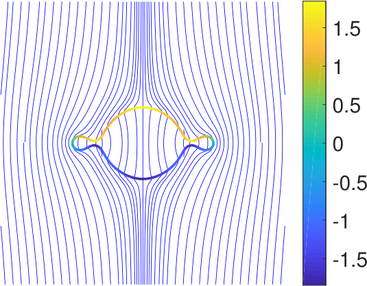
When an arbitrarily shaped vesicle is subjected to uniform electric field, it is known to transform into either a prolate shape or an oblate shape at equilibrium \citepriske2005electro, Sadik2011. Since ours is a 2D construct, we refer to ellipses whose major axis aligns with the electric field direction as “prolates”; similarly, those whose minor axis aligns as “oblates”. A classical observation in vesicle EHD studies is the prolate-oblate-prolate (POP) transition that arises in certain parameter regimes. Figure 1(a) illustrates the POP transition simulated using our numerical method.
Three conditions are generally required for a vesicle to undergo POP transition: 1) is very small so that the vesicle membrane acts more like a capacitor than a conductor, 2) is less than one and 3) is strong enough. Since , charges accumulate faster on the membrane exterior initially, thereby, the vesicle appears to be negatively charged at the top and positively charged at the bottom, leading to a compressional force from the applied electric field and the vesicle transitions from a prolate to an oblate shape. At longer times, once the membrane, acting as a capacitor, is fully charged, the apparent charge becomes zero and the vesicle transforms back into a prolate shape, which minimizes the electrostatic energy \citepC5SM00585J.
A notable feature of the POP transition is the squaring effect—a transient shape of the vesicle with four smoothed corners (as can be observed in Figure 1(a))—which attracted attention of researchers due to its implications on electroporation. Since the reduced area of a square is around 0.785, a question naturally arises: What transient shapes would a vesicle with much lower reduced area assume? In Figure 1(b), we illustrate the POP transition of a vesicle with . Since the fluid incompressibility acts to preserve its enclosed area, the vesicle forms small protrusions or “buds” to sustain the electrical compression forces. Figure 2 shows more details of this bud formation phase. The tension becomes negative, as expected, in the neck region of the buds. These intermediary shapes are reminiscent of those obtained by growing microtubules within the vesicles \citepfygenson1997mechanics; the notable feature here, however, is that only body forces are applied as opposed to local microtubule-membrane forces.

We further characterize the POP mechanism in Figure 3 for different reduced areas. In all the cases, we observe that there exists some critical field strength for POP transition to happen (e.g., from the figure, for , corresponding to respectively). On the other hand, when the field strength is weak, the vesicle remains a prolate and when the membrane conductivity is high, it transitions to an equilibrium oblate shape. These results are in qualitative agreement with [McConnell et al.(2015)McConnell, Vlahovska, and Miksis], where similar phase diagrams were presented but only for higher reduced area vesicles. Thus the phase diagrams in Figure 3 show that the POP mechanism works consistently for different .
Finally, in the case when , the EHD forces act to extend the vesicle and it remains a prolate throughout the simulation.
3.2 Electro-rheology in the dilute limit
We next look at the combined effect of an imposed shear flow and a DC electric field on a single vesicle. In the presence of both fields, the dynamics is characterized by a competition between the electrical and hydrodynamical shear stresses and the migration of electric charges along the vesicle membrane.
Figure 4 shows the rheological properties of a vesicle subjected to an applied linear shear and an applied uniform electric field. In this case, where the membrane has non-zero , we observe that the vesicles with different reduced areas all stabilize into a tank-treading motion and that the tank-treading speed and angle of inclination are affected nonlinearly by the conductivity ratio . Note that as is increased, the vesicle tries to align with the electric field direction and away from the direction of shear, presenting higher resistance to the imposed flow and hence leading to higher effective viscosity. Here, the effective viscosity is computed using the usual formula \citeprahimian10:
| (14) |
is the area of the vesicle and represents the perturbation in the stress due to membrane forces. After the vesicle reaches a steady-state, the effective viscosity is measured over an arbitrary time interval .
We further characterize the rheology in Figure 5 by plotting the effective viscosity as is varied. Highly deflated vesicles prominently display shear-rate and -dependent rheology since their shapes at equilibrium tank-treading dynamics are different, thereby, presenting varied resistance to applied shear.
In the case when is set to zero, the rheological behavior becomes much more complex, primarily because of the tendency of vesicles to undergo a POP transition while at the same time tank-tread due to the applied shear. For different values of and , we observed various behaviors such as tumbling, staggering (tank-treading with periodically varying inclination angles), “mirrored” tank-treading (tank-treading in the opposite direction and with inclination against the applied shear direction), and even chaotic staggering. A detailed analysis and characterization of these dynamics are beyond the scope of the present work and will be reported at a later date.
3.3 Two-body EHD interactions
Next we present results from simulation of two-body vesicle interactions in applied electric field and in the absence of imposed flow. As before, we assume that the viscosity and permittivity of the interior and exterior fluids are the same. We set the initial shape of both the vesicles to be identical and their initial location not symmetric with respect to the electric field direction11 1 When they are aligned along , they simply attract each other (after transient shape changes) and when aligned in the perpendicular direction, they simply repel each other—both results are consequences of one vesicle appearing to the other as a dipole with same orientation.. We apply a DC electric field, pointing upwards, strong enough to cause the POP transition when (i.e., ). Under these conditions, the different representative classes of dynamics observed are summarized in Figure 6.
The complex nature of these pairwise interactions can be understood from three predominant, competing mechanisms: (i) The electrically-driven vesicle alignment due to one vesicle appearing as a dipole (to leading order) in the far-field electrical disturbance produced by the second vesicle. The two vesicles always tend to form a chain along the direction of dipole orientation; (ii) The EHD flow induced by the tangential electrical stresses at the fluid-vesicle interfaces, driving the vesicles to rotate about each other; (iii) The prolate-oblate deformation mentioned in Section 3.1, generating extensional flows around each vesicle.
First, let us consider the case of i.e., the vesicle membranes are impermeable to charges. Three different types of dynamics can be observed from Figure 6. The first is chain formation, observed when is small enough, wherein, pronounced deformation, due to mechanism (iii), induces flows that dominate the circulatory flow of mechanism (ii). Thereby, it completely halts the tank-treading motion. At the end of their POP cycle, both vesicles become almost vertically-aligned. Then, mechanism (i) slowly drives them to form a stable chain. From our numerical experiments, we noticed that the thin layer of fluid between the vesicles gets continuously drained albeit at a very slow pace (distance between them decays exponentially with time).
The second type is a circulatory motion, observed when is large enough, wherein, mechanism (iii) becomes negligible. As the two vesicles move to form a chain, mechanism (ii) causes both of them to tank-tread. Consequently, the induced disturbance flow on each vesicle becomes dominant and they start to rotate about each other. The tank-treading motion also causes the vesicles to appear as tilted dipoles, so they tend to form a tilted chain. The circulatory motion is periodically reinforced by the tilted-chain formation process. The direction of rotation depends on the net torque on each vesicle, which has opposite orientations for and .
The last type is an oscillatory motion, where the two vesicles form an unstable chain and oscillate about each other. This is a transitional situation between the first two types, observed when is between the values of those types. In this case, neither the circulatory flow of mechanism (ii) is strong enough to keep vesicles rotating about each other nor the deformational flow of mechanism (iii) is strong enough to completely halt the rotations. The two vesicles tend to form a chain that is periodically tilted one way or the other; each time the vesicles passing a tilted-chain position, tank-treading slows down and the dipole orientation oscillates back. Therefore, mechanisms (i) and (ii) collaborate to keep the vesicles oscillating near the vertical chain position.
On the other hand, the dynamics are much simpler when the membrane is permeable to charges i.e., . After a very short period of initial charging, the electric stresses become almost normal to the surface of each vesicle, so mechanism (ii) doesn’t arise at all. By mechanism (iii) the vesicles eventually become oblate when (with strong enough ) and become prolate when , and mechanism (i) drives the vesicles to form a vertical chain.
Sensitivity to positions and shapes. Note that all of the aforementioned dynamics are insensitive to the initial offset or shapes of the vesicles. In Figure 8, we demonstrate that for different initial angular offsets from the aligned position, the vesicles undergo the same type of pairwise interaction that corresponds to the given and . Furthermore, Figure 9 shows that the similar kind of dynamics are observed for vesicles with different reduced areas, therefore, the pairwise EHD interaction mechanisms appear to be consistent for highly-deflated or close-to-circular vesicles.
Continuous transition. Finally, we note that the dynamics transitioning from to , as shown in Figure 6, are not abrupt. To illustrate this, we show in Figure 10 the pairwise dynamics of vesicles with , demonstrating a continuous transition from a chain of prolates () to a chain of oblates (); for certain intermediate values of , one can even observe interesting kidney-like shapes as well as decaying oscillations of the vesicles as they settle into their equilibrium shapes.
4 Conclusions
We investigated the pairwise dynamics and rheology of vesicles in DC electric fields using a boundary integral method. Our method is shown to reproduce previous results on isolated vesicle EHD and can be extended in a trivial manner to study the EHD of large number of vesicles. We showed that much richer set of pairwise interactions can be observed when the membranes are impermeable to charges. This is somewhat unique to vesicle EHD compared to other systems such as drops \citepbaygents1998electrohydrodynamic, driven mainly by the capacitative nature of the membranes. However, we explored only a small fraction of the possible dynamics; relaxing our simplifying assumptions—varying the viscosity and permittivity contrasts, imposing an AC electric field, accounting for charge convection along the membrane—is expected to enrich the space much further. We are currently exploring these as well as analyzing the collective dynamics of dense suspensions in periodic domains. Another important direction we are currently pursuing is to extend our numerical scheme to handle more general EHD models such as those discussed in the recent work of [Mori and Young(2018)].
References
- [Barnett et al.(2015)Barnett, Wu, and Veerapaneni] Alex Barnett, Bowei Wu, and Shravan Veerapaneni. Spectrally accurate quadratures for evaluation of layer potentials close to the boundary for the 2d stokes and laplace equations. SIAM Journal on Scientific Computing, 37(4):B519–B542, 2015.
- [Baygents et al.(1998)Baygents, Rivette, and Stone] JC Baygents, NJ Rivette, and HA Stone. Electrohydrodynamic deformation and interaction of drop pairs. Journal of Fluid Mechanics, 368:359–375, 1998.
- [Fygenson et al.(1997)Fygenson, Marko, and Libchaber] Deborah Kuchnir Fygenson, John F Marko, and Albert Libchaber. Mechanics of microtubule-based membrane extension. Physical review letters, 79(22):4497, 1997.
- [Hsiao and Wendland(2008)] George C Hsiao and Wolfgang L Wendland. Boundary integral equations, volume 164. Springer, 2008.
- [Hu et al.(2016)Hu, Lai, Seol, and Young] Wei-Fan Hu, Ming-Chih Lai, Yunchang Seol, and Yuan-Nan Young. Vesicle electrohydrodynamic simulations by coupling immersed boundary and immersed interface method. Journal of Computational Physics, 317:66–81, 2016.
- [Kolahdouz and Salac(2015)] Ebrahim M Kolahdouz and David Salac. Dynamics of three-dimensional vesicles in dc electric fields. Physical Review E, 92(1):012302, 2015.
- [Kress(1999)] R. Kress. Linear Integral Equations. Number v. 82 in Applied Mathematical Sciences. Springer New York, 1999.
- [McConnell et al.(2013)McConnell, Miksis, and Vlahovska] Lane C McConnell, Michael J Miksis, and Petia M Vlahovska. Vesicle electrohydrodynamics in dc electric fields. IMA Journal of Applied Mathematics, 2013.
- [McConnell et al.(2015)McConnell, Vlahovska, and Miksis] Lane C. McConnell, Petia M. Vlahovska, and Michael J. Miksis. Vesicle dynamics in uniform electric fields: squaring and breathing. Soft Matter, 11:4840–4846, 2015. doi: 10.1039/C5SM00585J. URL http://dx.doi.org/10.1039/C5SM00585J.
- [Mori and Young(2018)] Yoichiro Mori and Y.-N. Young. From electrodiffusion theory to the electrohydrodynamics of leaky dielectrics through the weak electrolyte limit. Journal of Fluid Mechanics, 855:67–130, 2018. doi: 10.1017/jfm.2018.567.
- [Nganguia and Young(2013)] H Nganguia and Y-N Young. Equilibrium electrodeformation of a spheroidal vesicle in an ac electric field. Physical Review E, 88(5):052718, 2013.
- [Perrier et al.(2017)Perrier, Rems, and Boukany] Dayinta L Perrier, Lea Rems, and Pouyan E Boukany. Lipid vesicles in pulsed electric fields: Fundamental principles of the membrane response and its biomedical applications. Advances in Colloid and Interface Science, 2017.
- [Rahimian et al.(2010)Rahimian, Veerapaneni, and Biros] A. Rahimian, S. K. Veerapaneni, and G. Biros. Dynamic simulation of locally inextensible vesicles suspended in an arbitrary two-dimensional domain, a boundary integral method. J. Comput. Phys., 229(18):6466–6484, 2010. ISSN 0021-9991.
- [Riske and Dimova(2005)] Karin A Riske and Rumiana Dimova. Electro-deformation and poration of giant vesicles viewed with high temporal resolution. Biophysical journal, 88(2):1143–1155, 2005.
- [Ristenpart et al.(2010)Ristenpart, Vincent, Lecuyer, and Stone] William D Ristenpart, Olivier Vincent, Sigolene Lecuyer, and Howard A Stone. Dynamic angular segregation of vesicles in electrohydrodynamic flows. Langmuir, 26(12):9429–9436, 2010.
- [Sadik et al.(2011)Sadik, Li, Shan, Shreiber, and Lin] Mohamed Sadik, Jianbo Li, Jerry Shan, David Shreiber, and Hao Lin. Vesicle deformation and poration under strong dc electric fields. Physical Review E, 83(6), June 2011. ISSN 1539-3755. doi: 10.1103/PhysRevE.83.066316. URL http://pre.aps.org/abstract/PRE/v83/i6/e066316.
- [Salipante and Vlahovska(2014)] Paul F Salipante and Petia M Vlahovska. Vesicle deformation in dc electric pulses. Soft matter, 10(19):3386–3393, 2014.
- [Schwalbe et al.(2011)Schwalbe, Vlahovska, and Miksis] Jonathan T Schwalbe, Petia M Vlahovska, and Michael J Miksis. Vesicle electrohydrodynamics. Physical Review E, 83(4):046309, 2011.
- [Veerapaneni et al.(2009)Veerapaneni, Gueyffier, Zorin, and Biros] S. K. Veerapaneni, D. Gueyffier, D. Zorin, and G. Biros. A boundary integral method for simulating the dynamics of inextensible vesicles suspended in a viscous fluid in 2D. Journal of Computational Physics, 228(7):2334–2353, 2009.
- [Veerapaneni(2016)] Shravan Veerapaneni. Integral equation methods for vesicle electrohydrodynamics in three dimensions. Journal of Computational Physics, 326:278–289, 2016.
- [Vlahovska et al.(2009)Vlahovska, Gracia, Aranda-Espinoza, and Dimova] Petia M Vlahovska, Ruben Serral Gracia, Said Aranda-Espinoza, and Rumiana Dimova. Electrohydrodynamic model of vesicle deformation in alternating electric fields. Biophysical journal, 96(12):4789–4803, 2009.
- [Zhang et al.(2013)Zhang, Zahn, Tan, and Lin] Jia Zhang, Jeffrey D Zahn, Wenchang Tan, and Hao Lin. A transient solution for vesicle electrodeformation and relaxation. Physics of Fluids (1994-present), 25(7):071903, 2013.