跳到论文正文
W Papers独立论文阅读器 arXiv:1801.06470 论文正文 计算阅读时间 · 0%
引用这篇论文根据当前论文元数据生成,正式投稿前建议核对。


License: arXiv.org perpetual non-exclusive license
arXiv:1801.06470v2 [math.AP] 13 May 2018

Stability estimates for systems with small cross-diffusionThanks: Maria Bruna was supported by the L’Oréal UK and Ireland Fellowship For Women In Science.Thanks: Luca Alasio was supported by the Engineering and Physical Sciences Research Council grant [EP/L015811/1].

Luca Alasio , Maria Bruna and Yves Capdeboscq
Abstract.

We discuss the analysis and stability of a family of cross-diffusion boundary value problems with nonlinear diffusion and drift terms. We assume that these systems are close, in a suitable sense, to a set of decoupled and linear problems. We focus on stability estimates, that is, continuous dependence of solutions with respect to the nonlinearities in the diffusion and in the drift terms. We establish well-posedness and stability estimates in an appropriate Banach space. Under additional assumptions we show that these estimates are time independent. These results apply to several problems from mathematical biology; they allow comparisons between the solutions of different models a priori. For specific cell motility models from the literature, we illustrate the limit of the stability estimates we have derived numerically, and we document the behaviour of the solutions for extremal values of the parameters.

Key words and phrases: 
Cross diffusion, Continuous dependence, Quasilinear parabolic systems
1991 Mathematics Subject Classification
35K55, 35B30, 35Q92, 65M15

1. Introduction

1.1. Background and motivation

In this paper we analyse a class of nonlinear cross-diffusion systems of PDEs which model multi-species populations in presence of short-range interactions between individuals. We assume that these systems are close, in a suitable sense, to decoupled sets of linear parabolic evolution problems. Such problems arise in many applications in mathematical biology, such as chemotactic cell migration, ion transport through cell membranes, and spatial segregation in interacting species. The strength of the interactions (and therefore of the nonlinear terms) is quantified with a small parameter ϵ\epsilon, so that when ϵ=0\epsilon=0 the system becomes diagonal and linear. The biological justification for these models comes from weakly-interacting species, whereby interactions between populations (such as excluded-volume or chemotactic interactions) are present but are not dominant over the isolated species behaviour.

The cross-diffusion systems we are interested in have the form

(1a) ∂tu−div[𝔇(t,x,u)∇u−𝔉(t,x,u)u]=0,inΩ,t>0,\partial_{t}u-\div\left[\mathfrak{D}(t,x,u)\nabla u-\mathfrak{F}(t,x,u)u\right]=0,\quad\text{in}\quad\Omega,t>0,
with boundary and initial conditions
(1b) [𝔇(t,x,u)∇u−𝔉(t,x,u)u]⋅ν\displaystyle\left[\mathfrak{D}(t,x,u)\nabla u-\mathfrak{F}(t,x,u)u\right]\cdot\nu =0,\displaystyle=0, on∂Ω,t>0,\displaystyle\text{on}\quad\partial\Omega,t>0,
(1c) u⁡(0,⋅)\displaystyle u(0,\cdot) =u0,\displaystyle=u^{0}, inΩ,\displaystyle\text{in}\quad\Omega,

where Ω\Omega is a smooth, bounded, and connected domain in ℝd\mathbb{R}^{d} (d=1,2,3d=1,2,3), ν\nu denotes the outward normal on ∂Ω\partial\Omega, and u=(u1,…,um)u=(u_{1},\dots,u_{m}) is the vector of densities of each species. The divergence div\div and gradient ∇\nabla represent derivatives with respect to the dd spatial variables. Here 𝔇⁡(t,x,u)\mathfrak{D}(t,x,u) and 𝔉⁡(t,x,u)\mathfrak{F}(t,x,u) are m×mm\times m matrices of diffusion tensors and drift vectors, respectively (see (12) for further details). In particular, the entries of the diffusion tensor 𝔇\mathfrak{D} may be scalars in the case of isotropic diffusion, or d×dd\times d tensors in the case of anisotropic diffusion. The drift matrix elements 𝔉i​j\mathfrak{F}_{ij} are d−d-dimensional vectors. In our class of cross-diffusion systems, the matrices 𝔇\mathfrak{D} and 𝔉\mathfrak{F} are close to matrices that are diagonal and independent of uu, that is, they can be written in the form

(2) 𝔇⁡(t,x,u)\displaystyle\mathfrak{D}(t,x,u) =𝔇(0)​(t,x)+ϵ​𝔇(1)​(t,x,u)+O⁡(ϵ2),\displaystyle=\mathfrak{D}^{(0)}(t,x)+\epsilon\mathfrak{D}^{(1)}(t,x,u)+O(\epsilon^{2}),
𝔉⁡(t,x,u)\displaystyle\mathfrak{F}(t,x,u) =𝔉(0)​(t,x)+ϵ​𝔉(1)​(t,x,u)+O⁡(ϵ2),\displaystyle=\mathfrak{F}^{(0)}(t,x)+\epsilon\mathfrak{F}^{(1)}(t,x,u)+O(\epsilon^{2}),

where ϵ\epsilon is a small parameter.

The focus of this paper is to study the stability of the solutions to (1) under perturbations of order ϵ\epsilon. We establish that the solutions depend continuously on the nonlinearities 𝔇(1)\mathfrak{D}^{(1)} and 𝔉(1)\mathfrak{F}^{(1)} for ϵ\epsilon small enough. The cross-diffusion model (1) is a non-linear system, and this combines two types of difficulties, namely the non-linearity and the fact that fully coupled parabolic systems of equations do not enjoy, in general, the same smoothness properties as parabolic equations (see, for example, [10, Chap. 9] , and [11]). Our results are detailed in Proposition 1.5 and Theorem 1.7. They are quantitative, in the sense that we provide a bound on ϵ\epsilon below which our perturbation result applies. The novelty of our analysis consists in the unified approach to the study of regularity and stability properties in “strong” Sobolev norms for a relatively wide class of nonlinear cross-diffusion systems.

Our stability estimate uses the underlying regularity of the system, which, as we will see, it inherits from the leading order model, consisting of decoupled linear evolution equations. We show that for small perturbations at least some of the regularity is preserved and, using a fixed point argument, we deduce a stability estimate with respect to the nonlinearities of the model.

Similar results concerning nonlinear systems where interactions between species (or components) are limited to lower order term (so-called weakly coupled systems) are available in the work of Camilli and Marchi [5]. They extend the results available for scalar equations in terms of continuous dependence estimates in the sup\sup norm using the doubling variable method [14] and viscosity solutions. Their results do not apply to fully coupled systems with cross diffusion present such as the ones we are considering. Continuous dependence for fully coupled quasilinear systems was studied by Cannon, Ford and Lair [6]. They established existence and uniqueness, following arguments of Ladyzhenskaya, Solonnikov, and Ural’tseva [15] in larger Sobolev spaces (weaker norms). They derive stability estimates under additional integrability properties assumptions for the gradients. We establish existence and uniqueness in stronger norms, removing the need of additional regularity assumptions.

There are several models, especially in mathematical biology, that fit into the class of systems (1) and (2). This is the case for models describing the transport of cells or ions while accounting for the finite-size of particles [3, 4, 21, 17]. These models were derived from stochastic agent-based models assuming that the concentration of cells or ions is not too large, so that the transport dominates over the finite-size interactions between cells or ions. The diffusion and drift matrices become density-dependent due to the interactions, but this correction is small since it scales with the excluded volume in the system. Below we present three of such models, and show how they fit into our framework.

Example 1.1 (Random walk on a lattice with size exclusion).

A cross-diffusion model for two interacting species was employed to describe the motility of biological cells by Simpson et al. [21] or ion transport by Burger et al. [4]. The models were derived assuming that particles are restricted to a regular square lattice and undergo a simple exclusion random walk, in which a particle can only jump to a site if it is presently unoccupied. In order to obtain a continuum model such as (1) from these so-called lattice-based models, it is generally assumed that the occupancies of adjacent sides are independent, so that the jumping probabilities take a simple form and do not require correlation functions [4, 21]. Clearly, such an approximation is poor when the overall occupancy of the lattice is high. As a result, these models are generally considered valid for low-lattice occupancies.

The models in [4, 21] consider two species of equal size, whose diameter is given by the lattice spacing ε\varepsilon, that undergo a random walk with isotropic diffusion DiD_{i} and external potential Vi​(x)V_{i}(x), for i=1,2i=1,2 (the jumping rates increase with DiD_{i} and the jumps are biased in the direction of −∇Vi​(x)-\nabla V_{i}(x)). There are N1N_{1} particles of the first species, and N2N_{2} of the second species. Under these assumptions, a cross-diffusion model of the form (1) is obtained, where the population densities u1​(t,x)u_{1}(t,x) and u2​(t,x)u_{2}(t,x) represent the probability that a particle from first or second species respectively is at x∈Ωx\in\Omega at time tt. The diffusion and drift matrices are given by [4]

(3a) 𝔇⁡(u)=(D1​(1−ϵ​N¯2​u2)ϵ​D1​N¯2​u1ϵ​D2​N¯1​u2D2​(1−ϵ​N¯1​u1)),\mathfrak{D}(u)=\begin{pmatrix}D_{1}(1-\epsilon\bar{N}_{2}u_{2})&\epsilon D_{1}\bar{N}_{2}u_{1}\\ \epsilon D_{2}\bar{N}_{1}u_{2}&D_{2}(1-\epsilon\bar{N}_{1}u_{1})\end{pmatrix},
(3b) 𝔉⁡(u)=(−∇V1​(1−ϵ​N¯1​u1)ϵN¯2u1∇V1ϵN¯1u2∇V2−∇V2​(1−ϵ​N¯2​u2)),\mathfrak{F}(u)=\begin{pmatrix}-\nabla V_{1}(1-\epsilon\bar{N}_{1}u_{1})&\epsilon\bar{N}_{2}u_{1}\nabla V_{1}\\ \epsilon\bar{N}_{1}u_{2}\nabla V_{2}&-\nabla V_{2}(1-\epsilon\bar{N}_{2}u_{2})\end{pmatrix},

where ϵ=(N1+N2)​εd/|Ω|≪1\epsilon=(N_{1}+N_{2})\varepsilon^{d}/|\Omega|\ll 1 represents the total volume fraction of the lattice occupied by particles and N¯i=Ni/(N1+N2)\bar{N}_{i}=N_{i}/(N_{1}+N_{2}). We have written (3) in a form consistent with our notations, which differ slightly from those used in [4]. Global existence for such model was shown in [7]. In that paper, as in most works using lattice-based models, the continuum model is written in terms of the volume concentrations u^i\hat{u}_{i}, so that the mass of u^i\hat{u}_{i} equals the total volume occupied by species ii (that is, ∫Ωu^i​(t,x)​𝑑x=Ni​εd/|Ω|\int_{\Omega}\hat{u}_{i}(t,x){\mathrm{d}}x=N_{i}\varepsilon^{d}/|\Omega|). We write (3) in terms of probability densities uiu_{i}, which implies that ∫Ωui​𝑑x=1\int_{\Omega}u_{i}{\mathrm{d}}x=1. The two quantities are related by the identity u^i=N¯i​ϵ​ui\hat{u}_{i}=\bar{N}_{i}\epsilon u_{i}. The potentials appearing in (3b), ViV_{i}, are not rescaled by the diffusion coefficient as it is done in [4]. The number of species can take any values provided that ϵ\epsilon, is small. The matrices in (3) are of the form (2) that we consider in this paper. There are also other lattice-based models that fit well into such framework, such as that derived by Shigesada et al. [20] to describe spatial segregation of interacting animal populations.

Example 1.2 (Brownian motion with size exclusion).

A cross-diffusion model for two interacting species of diffusive particles was obtained by Bruna and Chapman for d=2,3d=2,3 in [3], starting from a system with two types of Brownian hard spheres. The population densities ui​(t,x)u_{i}(t,x), i=1,2i=1,2, represent the probability that a particle of species ii is at x∈Ωx\in\Omega at time tt, and so ∫Ωui​(t,x)​𝑑x=1\int_{\Omega}u_{i}(t,x){\mathrm{d}}x=1. The model assumes there are NiN_{i} particles of species ii, of diameter εi\varepsilon_{i} and isotropic diffusion constant DiD_{i}. The position XiX_{i} of each particle in species ii evolves in time according to the stochastic differential equation

(4) d​Xi​(t)=2​Di​d​W​(t)−∇Vi​(Xi​(t))​d​t,\mathrm{d}X_{i}(t)=\sqrt{2D_{i}}\mathrm{d}{W}(t)-\nabla V_{i}(X_{i}(t))\mathrm{d}t,

where i=1i=1 or 2, and WW are independent, dd-dimensional standard Brownian motions. Reflective boundary conditions are imposed whenever two particles are in contact (‖Xi−Xj‖=(εi+εj)/2\|X_{i}-X_{j}\|=(\varepsilon_{i}+\varepsilon_{j})/2, when XiX_{i} and XjX_{j} are of type ii and jj, respectively), as well as on the boundary of the domain ∂Ω\partial\Omega.

The cross-diffusion model is derived using the method of matched asymptotic expansions under the assumption that the volume fraction of the system is small, or equivalently, that (N1​ε1d+N2​ε2d)/|Ω|∼ϵ≪1(N_{1}\varepsilon_{1}^{d}+N_{2}\varepsilon_{2}^{d})/|\Omega|\sim\epsilon\ll 1, where ϵ\epsilon is defined as in Example 1.1 with ε=(ε1+ε2)/2\varepsilon=(\varepsilon_{1}+\varepsilon_{2})/2. When the number of particles in each species is large, the cross-diffusion model in [3] is of the form (1), with diffusion matrix

(5a) 𝔇⁡(u)=(D1​(1+ϵ​a1​u1−ϵ​c1​u2)ϵ​D1​b1​u1ϵ​D2​b2​u2D2​(1+ϵ​a2​u2−ϵ​c2​u1)),\mathfrak{D}(u)=\begin{pmatrix}D_{1}(1+\epsilon a_{1}u_{1}-\epsilon c_{1}u_{2})&\epsilon D_{1}b_{1}u_{1}\\ \epsilon D_{2}b_{2}u_{2}&D_{2}(1+\epsilon a_{2}u_{2}-\epsilon c_{2}u_{1})\end{pmatrix},
and drift matrix
(5b) 𝔉⁡(u)=(−∇V1ϵc1∇(V1−V2)u1ϵc2∇(V2−V1)u2−∇V2).\mathfrak{F}(u)=\begin{pmatrix}-\nabla V_{1}&\epsilon c_{1}\nabla(V_{1}-V_{2})u_{1}\\ \epsilon c_{2}\nabla(V_{2}-V_{1})u_{2}&-\nabla V_{2}\end{pmatrix}.

The parameters ai,bi,cia_{i},b_{i},c_{i} (i=1,2i=1,2) are all positive numbers that depend on the problem dimension, particle sizes, numbers, and relative diffusion coefficients (see specific values in Section 3). Model (5) also fits into the form (2), with ϵ=0\epsilon=0 when particles are non-interactive (point particles) and evolve according to two decoupled linear drift-diffusion equations.

Example 1.3 (Asymptotic gradient-flow structures).

Certain cross-diffusion systems possess a formal gradient-flow structure, that is, they can be formulated as

(6) ∂tu−∇⋅(M∇δ​Eδ​u)=0,\partial_{t}u-\nabla\cdot\left(M\nabla\frac{\delta E}{\delta u}\right)=0,

where M∈ℝm×mM\in\mathbb{R}^{m\times m} is known as mobility matrix and δ​E/δ​u\delta E/\delta u is the variational derivative of the entropy (or free energy) function E⁡[u]E[u]. While the underlying microscopic model (4) of Example 1.2 has a natural entropy, in [2] it was noted that model (5) does not have an obvious gradient-flow structure, but that it is close to one that does have such convenient structure. More specifically, consider the following entropy

(7a) Eϵ​[u]=∫Ω[u1​log⁡u1+u2​log⁡u2+u1​V1D1+u2​V2D2+ϵ2​(a1​u12+2​a12​u1​u2+a2​u22)]​𝑑x,E_{\epsilon}[u]=\int_{\Omega}\bigg[u_{1}\log u_{1}+u_{2}\log u_{2}+u_{1}\frac{V_{1}}{D_{1}}+u_{2}\frac{V_{2}}{D_{2}}+\frac{\epsilon}{2}\left(a_{1}u_{1}^{2}+2a_{12}u_{1}u_{2}+a_{2}u_{2}^{2}\right)\bigg]{\mathrm{d}}x,
with a12=(d−1)​(c1+c2)a_{12}=(d-1)(c_{1}+c_{2}), and the mobility matrix
(7b) Mϵ​(u)=(D1​u1​(1−ϵ​c1​u2)D1​c2​ϵ​u1​u2D2​c1​ϵ​u1​u2D2​u2​(1−c2​ϵ​u1)).M_{\epsilon}(u)=\begin{pmatrix}D_{1}u_{1}(1-\epsilon c_{1}u_{2})&D_{1}c_{2}\epsilon u_{1}u_{2}\\ D_{2}c_{1}\epsilon u_{1}u_{2}&D_{2}u_{2}(1-c_{2}\epsilon u_{1})\end{pmatrix}.

The cross-diffusion system (1) with diffusion and drift matrices (5) and N1=N2N_{1}=N_{2}11 1 In [2] the more general case when N1≠N2N_{1}\neq N_{2} was also considered, by writing the system in terms of number densities Ni​uiN_{i}u_{i}., can be rewritten as

(8) ∂tu=∇⋅(Mϵ∇δ​Eϵδ​u−ϵ2G),\partial_{t}u=\nabla\cdot\left(M_{\epsilon}\nabla\frac{\delta E_{\epsilon}}{\delta u}-\epsilon^{2}G\right),

where G=G⁡(u,∇u)G=G(u,\nabla u) (see more details in Section 3). In particular, the discrepancy between the system in Example 1.2 and the gradient-flow induced by (7) is of order ϵ2\epsilon^{2}, an order higher than that of the model.22 2 Systems (1)-(5) and (6)-(7) are in fact identical when both species have the same particle sizes, ε1=ε2\varepsilon_{1}=\varepsilon_{2}, and diffusivities, D1=D2D_{1}=D_{2}, since GG vanishes in that particular case. Does this legitimise the use of (7) as a gradient-flow structure of the system? Having a formal gradient-flow structure can facilitate the analysis of cross-diffusion models [13]. The gradient-flow model (6)-(7) was studied in [2]; stability, uniqueness of the stationary solutions, and a global-in-time existence result was shown.

It is natural to ask whether the approximation argument in Example 1.3 can be made rigorous, and, more generally if minor changes in the models can be safely ignored. For instance, given a two-species biological system, does it matter if we choose a lattice-based model (like in Example 1.1), or an off-lattice model (like in Example 1.2 with equal particle number, size, diffusivity, etc.)? If so, can we quantify the differences? Lattice-based approaches have become very common, as they offer a simple way to derive continuum PDE models. They can be unrealistic since most biological transport processes modelled by these are not constrained on a lattice [18]. Nevertheless, if one is solely interested in the population-level behaviour of the system, is it worth using a more realistic off-lattice model? When is the even simpler model (linear advection-diffusion) sufficiently accurate? The aim of this paper is to answer these questions and quantify the differences between models of the form (1).

1.2. Outline of the results

As we are working with systems of equations, we use different indices to refer to the ambient space variables and the component or species number. Greek indices 1≤α,β≤d1\leq\alpha,\beta\leq d refer to directions in the ambient space, ℝd\mathbb{R}^{d}, for d=1,2,3d=1,2,3. Latin indices 1≤i,j≤m1\leq i,j\leq m are used to refer to the species number. The domain Ω\Omega where the problem is formulated is bounded, connected and of class C2C^{2} in ℝd\mathbb{R}^{d}. The outward normal on ∂Ω\partial\Omega is written ν\nu.

The parabolic models we consider are weak formulations of problems of the form

(9) ∂tui−∂α[𝔇i​jα​β​(t,x,u)​∂βuj−𝔉i​jα​(t,x,u)​uj]=0in Ω,[𝔇i​jα​β​(t,x,u)​∂βuj−𝔉i​jα​(t,x,u)​uj]⋅να=0on ∂Ω,u⁡(0,⋅)=u0in Ω,\displaystyle\begin{aligned} \partial_{t}u_{i}-\partial_{\alpha}\left[\mathfrak{D}_{ij}^{\alpha\beta}(t,x,u)\partial_{\beta}u_{j}-\mathfrak{F}_{ij}^{\alpha}(t,x,u)u_{j}\right]&=0&\text{in }&\Omega,\\ \left[\mathfrak{D}_{ij}^{\alpha\beta}(t,x,u)\partial_{\beta}u_{j}-\mathfrak{F}_{ij}^{\alpha}(t,x,u)u_{j}\right]\cdot\nu_{\alpha}&=0&\text{on }&\partial\Omega,\\ u(0,\cdot)&=u^{0}&\text{in }&\Omega,\end{aligned}

for 1≤i≤m,1\leq i\leq m,. The Einstein summation convention is used, that is, repeated indices are implicitly summed.

Our main result is a stability estimate for cross-diffusion systems that are close to diagonal, decoupled, linear diffusion problems. Our reference problem will be the weak formulation of

(10) ∂tui−∂α[Diα​β​(t,x)​∂βui−Fiα​(t,x)​ui]=0in Ω,[Diα​β​(t,x)​∂βui−Fiα​(t,x)​ui]⋅να=0on ∂Ω,u⁡(0,⋅)=u0in Ω,\displaystyle\begin{aligned} \partial_{t}u_{i}-\partial_{\alpha}\left[D_{i}^{\alpha\beta}(t,x)\partial_{\beta}u_{i}-F_{i}^{\alpha}(t,x)u_{i}\right]&=0&\text{in }&\Omega,\\ \left[D_{i}^{\alpha\beta}(t,x)\partial_{\beta}u_{i}-F_{i}^{\alpha}(t,x)u_{i}\right]\cdot\nu_{\alpha}&=0&\text{on }&\partial\Omega,\\ u(0,\cdot)&=u^{0}&\text{in }&\Omega,\end{aligned}

The initial datum u0u^{0} in (9) and (10) belongs to H2​(Ω)H^{2}(\Omega). Note that throughout the paper we write H2​(Ω)H^{2}(\Omega) for H2​(Ω,ℝm)H^{2}(\Omega;\mathbb{R}^{m}), and similarly for other spaces.

Compared to the general system (9), in (10) we have specified that 𝔇i​j=𝔉i​j=0\mathfrak{D}_{ij}=\mathfrak{F}_{ij}=0 if i≠ji\neq j, and 𝔇\mathfrak{D} and 𝔉\mathfrak{F} do not depend on uu. In Examples 1.1, 1.2, and 1.3, the reference problem corresponds to the case ϵ=0\epsilon=0, with Diα​β​(x,t)=δα​β​DiD_{i}^{\alpha\beta}(x,t)=\delta_{\alpha\beta}D_{i} and Fi=−∇ViF_{i}=-\nabla V_{i}. We allow time and space variations of the diffusion coefficients as it does not affect the analysis. We could also have safely included lower-order terms, but it would have resulted in somewhat longer and relatively routine developments. Additionally such terms do not appear in the three examples of interest.

System (10) is strongly parabolic, that is, there exist a positive constant λ\lambda such that for every t∈[0,∞)t\in[0,\infty), x∈Ωx\in\Omega and ξ∈ℝd\xi\in\mathbb{R}^{d}, there holds

(11) Diα​β(t,x)ξαξβ≥λ|ξ|2,i=1,…,m.D_{i}^{\alpha\beta}(t,x)\xi^{\alpha}\xi^{\beta}\geq\lambda\left|\xi\right|^{2},\quad i=1,\ldots,m.

Furthermore, we shall assume that DD is symmetric in the space indices α\alpha and β\beta.

We allow perturbations of system (10) scaled by a small parameter ϵ\epsilon. Namely we consider (9) with

(12) 𝔇i​jα​β​(t,x,u)=Diα​β​(t,x)+ϵ​ai​jα​β​(t,x)​ϕi​jα​β​(u),𝔉i​jα​(t,x,u)=Fiα​(t,x)+ϵ​bi​jα​(t,x)​ψi​jα​(u).\displaystyle\begin{aligned} \mathfrak{D}_{ij}^{\alpha\beta}(t,x,u)&=D_{i}^{\alpha\beta}(t,x)+\epsilon a_{ij}^{\alpha\beta}(t,x)\phi_{ij}^{\alpha\beta}(u),\\ \mathfrak{F}_{ij}^{\alpha}(t,x,u)&=F_{i}^{\alpha}(t,x)+\epsilon b_{ij}^{\alpha}(t,x)\psi_{ij}^{\alpha}(u).\end{aligned}

The variations of the coefficients aa and bb are of class C2C^{2} in time and space, that is,

(13) ‖(a,b)‖C2​([0,∞)×ℝd)≤M,\left\|\left(a,b\right)\right\|_{C^{2}\left([0,\infty)\times\mathbb{R}^{d}\right)}\leq M,

and the dependence on uu of the perturbations is also of class C2C^{2},

(14) ϕ,ψ∈C2​(ℝm)m×m,ϕ⁡(0)=ψ⁡(0)=0.\phi,\psi\in C^{2}\left(\mathbb{R}^{m}\right)^{m\times m},\qquad\phi(0)=\psi(0)=0.

Furthermore, we assume that DD and FF satisfy the bound

(15) ∑α,β,i‖Diα​β‖C1​([0,∞)×ℝd)+∑α,i‖Fiα‖C1​([0,∞)×ℝd)≤M.\sum_{\alpha,\beta,i}\|D_{i}^{\alpha\beta}\|_{C^{1}\left([0,\infty)\times\mathbb{R}^{d}\right)}+\sum_{\alpha,i}\|F_{i}^{\alpha}\|_{C^{1}\left([0,\infty)\times\mathbb{R}^{d}\right)}\leq M.

In the context of biological models, one is often interested in arbitrarily long behaviour and, in turn, convergence to a steady state. Along this line, we prove sharper estimates when the coefficients DD and FF of the reference problem (10) do not depend on time and FF is derived from a potential (as in Examples 1.1, 1.2, and 1.3). In particular, consider the following additional assumption:

  • (H)

    for each i∈{1,…,m}i\in\{1,\ldots,m\}, DiD_{i} is independent of time and there exists ViV_{i} such that Fi=−Di∇ViF_{i}=-D_{i}\nabla V_{i}.

Our estimates will be expressed in terms of the constants appearing in assumptions (11), (13), (14) and (15). More specifically, the following positive-valued functions will appear:

(16) Li\displaystyle L_{i} :\displaystyle: R→‖(ϕ,ψ)‖Ci​(BR​(0)¯)i=0,1,2,\displaystyle R\to\left\|\left(\phi,\psi\right)\right\|_{C^{i}\left(\overline{B_{R}(0)}\right)}\quad i=0,1,2,
(17) K0\displaystyle K_{0} :\displaystyle: R→M⁡(5​L0​(CS∞​R)+2​CS2​L1​(CS∞​R)​R),\displaystyle R\to M\left(5L_{0}\left({C_{S}^{\infty}}\,R\right)+2C_{S}^{2}L_{1}\left({C_{S}^{\infty}}\,R\right)R\right),
(18) K1\displaystyle K_{1} :\displaystyle: R→CS​M​(L1​(R)​R+L2​(R)​R2),\displaystyle R\to C_{S}M\left(L_{1}(R)R+L_{2}(R)R^{2}\right),
(19) K2\displaystyle K_{2} :\displaystyle: R→6​R​CT/∞​CS​max⁡((L0​(R)+L1​(R)​R),M⁡(1+R)),\displaystyle R\to 6RC_{T/\infty}C_{S}\max\left(\left(L_{0}(R)+L_{1}(R)R\right),M(1+R)\right),

where CS2{C_{S}^{2}}, CSC_{S}, and CS∞{C_{S}^{\infty}} depend on Ω\Omega and dd and are given by (32), (33), and (73) respectively. The constant CT/∞C_{T/\infty} determines the dependence on a final time T>0T>0 of our estimates and is given by

(20) CT/∞={CT when (H) does not applyC∞ when (H) applies,C_{T/\infty}=\left\{\begin{array}[]{rl}C_{T}&\textrm{ when {(H)} does not apply}\\ C_{\infty}&\textrm{ when {(H)} applies},\end{array}\right.

where CTC_{T} is given by (68) and depends on MM, Ω\Omega, L0L_{0}, L1L_{1} and TT only, and C∞C_{\infty} is specified in (69) and it depends on MM, Ω\Omega, L0L_{0} and L1L_{1} only – not TT. The upper bound ϵ0\epsilon_{0} on the range of values ϵ\epsilon allowed will be determined by means of the following function

(21) ϵ0:R→min⁡(12+2​K0​(R),11+K1​(R)).\epsilon_{0}:R\to\min\left(\frac{1}{2+2K_{0}(R)},\frac{1}{1+K_{1}(R)}\right).

Our first result, which is instrumental to our main theorem, provides an existence result and a regularity estimate for solutions of system (9). Given T>0T>0, we denote the parabolic cylinder by QT=(0,T)×ΩQ_{T}=(0,T)\times\Omega.

Definition 1.4.

We name W⁡(QT)W(Q_{T}) the Banach space of functions with two weak derivatives in space in L2​(Ω)L^{2}(\Omega) continuously in time, and one time derivative in H1​(QT)H^{1}(Q_{T}), that is,

W(QT)={u∈C([0,T];H2(Ω)),∂tu∈H1(QT)}.W\left(Q_{T}\right)=\left\{u\in C\left(\left[0,T\right];H^{2}(\Omega)\right),\partial_{t}u\in H^{1}\left(Q_{T}\right)\right\}.

We are now ready to state our first result, concerning existence and uniqueness of solutions of (9).

Proposition 1.5.

Assume that hypothesis (11), (12), (13), (14) and (15) hold. Consider u0∈W⁡(QT)u^{0}\in W(Q_{T}) satisfying the compatibility condition

(22) [𝔇i​jα​β​(t,x,u0)​∂βuj0−𝔉i​jα​(t,x,u0)​uj0]⋅ν=0on ​∂Ω,i=1,…,m.\left[\mathfrak{D}_{ij}^{\alpha\beta}(t,x,u^{0})\partial_{\beta}u^{0}_{j}-\mathfrak{F}_{ij}^{\alpha}(t,x,u^{0})u^{0}_{j}\right]\cdot\nu=0\quad\text{on }\partial\Omega,\quad i=1,\ldots,m.

Let

(23) Y0=CT/∞​‖u0‖H2​(Ω).Y_{0}=C_{T/\infty}\|u^{0}\|_{H^{2}(\Omega)}.

If ϵ<ϵ0​(Y0)\epsilon<\epsilon_{0}(Y_{0}), then system (9) admits a unique solution u∈W⁡(QT)u\in W(Q_{T}) and there holds

‖u‖W⁡(QT)≤Y0.\|u\|_{W(Q_{T})}\leq Y_{0}.
Remark 1.6.

Any compatible initial data in H2​(Ω)H^{2}(\Omega) is allowed, provided ϵ\epsilon is small enough. Note that the compatibility condition (22) holds for any initial data compactly supported in Ω\Omega. All ϵ\epsilon within the range [0,ϵ0​(Y0))[0,\epsilon_{0}(Y_{0})) are allowed, and the solution uu is bounded linearly by its initial condition. When assumption (H) holds, the solution is bounded for all times.

Our result holds for space dimension d=1,2d=1,2 and 33, but not above. Two embeddings are used in our proofs: L4​(Ω)⊂H1​(Ω)L^{4}(\Omega)\subset H^{1}(\Omega), which does not hold when d≥5d\geq 5, and L∞​(Ω)⊂H2​(Ω)L^{\infty}(\Omega)\subset H^{2}(\Omega), which does not hold when d≥4d\geq 4.

Our purpose is to establish a stability result under perturbations. Therefore we consider a second problem with 𝔇\mathfrak{D} and 𝔉\mathfrak{F} replaced by

(24) 𝔇~i​jα​β​(t,x,u)=Diα​β​(t,x)+ϵ​a~i​jα​β​(t,x)​ϕ~i​jα​β​(u),𝔉~i​jα​(t,x,u)=Fiα​(t,x)+ϵ​b~i​jα​(t,x)​ψ~i​jα​(u),\displaystyle\begin{aligned} \widetilde{\mathfrak{D}}_{ij}^{\alpha\beta}(t,x,u)&=D_{i}^{\alpha\beta}(t,x)+\epsilon\tilde{a}_{ij}^{\alpha\beta}(t,x)\tilde{\phi}_{ij}^{\alpha\beta}(u),\\ \widetilde{\mathfrak{F}}_{ij}^{\alpha}(t,x,u)&=F_{i}^{\alpha}(t,x)+\epsilon\tilde{b}_{ij}^{\alpha}(t,x)\tilde{\psi}_{ij}^{\alpha}(u),\end{aligned}

where a~,\tilde{a}, b~\tilde{b}, ϕ~\tilde{\phi} and ψ~\tilde{\psi} satisfy hypothesis (13), (14) and, without loss of generality,

‖(ϕ~,ψ~)‖Ci​(BR​(0)¯)≤Li​(R)for all0≤R,i=0,1,2.\big\|(\tilde{\phi},\tilde{\psi})\big\|_{C^{i}(\overline{B_{R}(0)})}\leq L_{i}(R)\quad\text{for all}\quad 0\leq R,\quad i=0,1,2.

for LiL_{i} defined in (16). Our main result is as follows.

Theorem 1.7.

Given u0,u~0∈H2​(Ω)u^{0},\tilde{u}^{0}\in H^{2}(\Omega) compactly supported in Ω\Omega, write

Y1=CT/∞​max⁡(‖u0‖H2​(Ω),‖u~0‖H2​(Ω)),Y_{1}=C_{T/\infty}\max\left(\|u^{0}\|_{H^{2}(\Omega)},\|{\tilde{u}}^{0}\|_{H^{2}(\Omega)}\right),

and assume ϵ<ϵ0​(Y1)\epsilon<\epsilon_{0}(Y_{1}) so that Proposition 1.5 applies for both sets of parameters. Let u∈W⁡(QT)u\in W(Q_{T}) be the solution of (9) and u~∈W⁡(QT)\tilde{u}\in W(Q_{T}) be the solution of (9) with 𝔇\mathfrak{D}, 𝔉\mathfrak{F} and u0u^{0} are replaced by 𝔇~\widetilde{\mathfrak{D}} and 𝔉~\widetilde{\mathfrak{F}} and u~0{\tilde{u}}^{0}, respectively. Then the following stability estimate holds:

(25) ‖u~−u‖W⁡(QT)≤Γ1​‖u~0−u0‖H2​(Ω)+ϵ​Γ2​(‖(a~,b~)−(a,b)‖C1​([0,∞)×ℝd)+‖(ϕ~,ψ~)−(ϕ,ψ)‖C1​(BY1​(0)¯)),\left\|\tilde{u}-u\right\|_{W(Q_{T})}\leq\Gamma_{1}\|{\tilde{u}}^{0}-u^{0}\|_{H^{2}(\Omega)}+\epsilon\Gamma_{2}\left(\|(\tilde{a},\tilde{b})-(a,b)\|_{C^{1}([0,\infty)\times\mathbb{R}^{d})}+\|(\tilde{\phi},\tilde{\psi})-(\phi,\psi)\|_{C^{1}\left(\overline{B_{Y_{1}}(0)}\right)}\right),

where Γ1=(1+K1​(Y1))​CT/∞\Gamma_{1}=(1+K_{1}(Y_{1}))C_{T/\infty}, Γ2=(1+K1​(Y1))​K2​(Y1)\Gamma_{2}=(1+K_{1}(Y_{1}))K_{2}(Y_{1}) and K1K_{1}, K2K_{2} are non decreasing functions given by (18), (19) respectively. They depend on Ω\Omega, MM, λ\lambda, L0L_{0}, L1L_{1} and L2L_{2} and CT/∞C_{T/\infty} only.

Theorem 1.7 implies, for example, that we can control the differences between the solutions of the models in Examples 1.1 and 1.2, by considering the differences in their respective diffusion and drift matrices, which appear at order ϵ\epsilon. Similarly, we can also use this result to predict the error we will make by approximating model (5) in Example 1.2 as the gradient flow in Example 1.3. Since the differences between models appear at order ϵ2\epsilon^{2} in this case, provided the initial data are equal, the error will be bounded and of order ϵ2\epsilon^{2} for all times (see Section 3).

Remark 1.8.

In Proposition 1.5 the compatibility condition (22) appears, which is automatically satisfied by compactly supported initial data as we have assumed in Theorem 1.7. However, Theorem 1.7 also holds (with the same proof) provided that u0u^{0} and u~0\tilde{u}^{0} satisfy the following four conditions:

[𝔇i​jα​β​(t,x,u0)​∂βuj0−𝔉i​jα​(t,x,u0)​uj0]⋅ν\displaystyle\left[\mathfrak{D}_{ij}^{\alpha\beta}(t,x,u^{0})\partial_{\beta}u^{0}_{j}-\mathfrak{F}_{ij}^{\alpha}(t,x,u^{0})u^{0}_{j}\right]\cdot\nu =0\displaystyle=0 on ​∂Ω,\displaystyle\text{on }\partial\Omega, i\displaystyle\quad i =1,…,m,\displaystyle=1,\ldots,m,
[𝔇i​jα​β​(t,x,u~0)​∂βu~j0−𝔉i​jα​(t,x,u~0)​u~j0]⋅ν\displaystyle\left[\mathfrak{D}_{ij}^{\alpha\beta}(t,x,\tilde{u}^{0})\partial_{\beta}\tilde{u}^{0}_{j}-\mathfrak{F}_{ij}^{\alpha}(t,x,\tilde{u}^{0})\tilde{u}^{0}_{j}\right]\cdot\nu =0\displaystyle=0 on ​∂Ω,\displaystyle\text{on }\partial\Omega, i\displaystyle i =1,…,m,\displaystyle=1,\ldots,m,
[𝔇~i​jα​β​(t,x,u0)​∂βuj0−𝔉~i​jα​(t,x,u0)​uj0]⋅ν\displaystyle\left[\widetilde{\mathfrak{D}}_{ij}^{\alpha\beta}(t,x,u^{0})\partial_{\beta}u^{0}_{j}-\tilde{\mathfrak{F}}_{ij}^{\alpha}(t,x,u^{0})u^{0}_{j}\right]\cdot\nu =0\displaystyle=0 on ​∂Ω,\displaystyle\text{on }\partial\Omega, i\displaystyle i =1,…,m,\displaystyle=1,\ldots,m,
[𝔇~i​jα​β​(t,x,u~0)​∂βu~j0−𝔉~i​jα​(t,x,u~0)​u~j0]⋅ν\displaystyle\left[\widetilde{\mathfrak{D}}_{ij}^{\alpha\beta}(t,x,\tilde{u}^{0})\partial_{\beta}\tilde{u}^{0}_{j}-\tilde{\mathfrak{F}}_{ij}^{\alpha}(t,x,\tilde{u}^{0})\tilde{u}^{0}_{j}\right]\cdot\nu =0\displaystyle=0 on ​∂Ω,\displaystyle\text{on }\partial\Omega, i\displaystyle i =1,…,m.\displaystyle=1,\ldots,m.

We choose to write the result for compactly supported initial data to improve readability.

2. Proof of Proposition 1.5 and Theorem 1.7

In Lemma 2.1, we derive an estimate for a linearisation of system (9).

Lemma 2.1.

Assume that 𝔇\mathfrak{D} and 𝔉\mathfrak{F} are given by (12), and that a,ba,b and ϕ,ψ\phi,\psi satisfy (13) and (14) respectively. Suppose that h∈W⁡(QT)h\in W(Q_{T}) satisfies

(26) ϵ​K0​(‖h‖W⁡(QT))<1,\epsilon K_{0}\left(\left\|h\right\|_{W\left(Q_{T}\right)}\right)<1,

where K0K_{0} is given by (17).

For all u0∈H2​(Ω)u^{0}\in H^{2}(\Omega) and f∈C⁡([0,T],H1​(QT))∩H1​(0,T,L2​(Ω))f\in C([0,T];H^{1}\left(Q_{T}\right))\cap H^{1}(0,T;L^{2}(\Omega)) such that

(27) [𝔇i​jα​β​(t,x,h)​∂βuj0−𝔉i​jα​(t,x,h)​uj0+fiα​(t=0)]⋅ν=0on ​∂Ω,i=1,…,m\left[\mathfrak{D}_{ij}^{\alpha\beta}(t,x,h)\partial_{\beta}u^{0}_{j}-\mathfrak{F}_{ij}^{\alpha}(t,x,h)u^{0}_{j}+f^{\alpha}_{i}(t=0)\right]\cdot\nu=0\quad\text{on }\partial\Omega,\quad i=1,\ldots,m

there exists a unique weak solution u∈W⁡(QT)u\in W(Q_{T}) to the linearised system

(28) ∂tui−∂α[𝔇i​jα​β​(t,x,h)​∂βuj−𝔉i​jα​(t,x,h)​uj+fiα]=0in ​𝒟′​(Ω),[𝔇i​jα​β​(t,x,h)​∂βuj−𝔉i​jα​(t,x,h)​uj+fiα]​να=0on ​∂Ω,i=1,…,mu⁡(0,x)=u0in ​Ω.\displaystyle\begin{aligned} \partial_{t}u_{i}-\partial_{\alpha}\left[\mathfrak{D}_{ij}^{\alpha\beta}(t,x,h)\partial_{\beta}u_{j}-\mathfrak{F}_{ij}^{\alpha}(t,x,h)u_{j}+f_{i}^{\alpha}\right]&=0&&\text{in }\mathcal{D}^{\prime}(\Omega),\\ \left[\mathfrak{D}_{ij}^{\alpha\beta}(t,x,h)\partial_{\beta}u_{j}-\mathfrak{F}_{ij}^{\alpha}(t,x,h)u_{j}+f_{i}^{\alpha}\right]\nu_{\alpha}&=0&&\text{on }\partial\Omega,\quad i=1,\ldots,m\\ u(0,x)&=u^{0}&&\text{in }\Omega.\end{aligned}

Furthermore, the solution map

(29) S:(h,u0,f)→u​, where ​u​ is the solution of (28),S:\left(h,u^{0},f\right)\to u\text{, where }u\text{ is the solution of \eqref{eq:parab-linear},}

satisfies

‖S⁡(h,u0,f)‖W⁡(QT)​[1−ϵ​K0​(‖h‖W⁡(QT))]≤12​CT/∞​(‖u0‖H2​(Ω)+‖f‖C⁡([0,T],H1​(QT))∩H1​(0,T,L2​(Ω))),\big\|S(h,u^{0},f)\big\|_{W(Q_{T})}\left[1-\epsilon K_{0}(\left\|h\right\|_{W(Q_{T})})\right]\leq\frac{1}{2}C_{T/\infty}\left(\|u^{0}\|_{H^{2}(\Omega)}+\left\|f\right\|_{C([0,T];H^{1}\left(Q_{T}\right))\cap H^{1}(0,T;L^{2}(\Omega))}\right),

where CT/∞>0C_{T/\infty}>0 is given by (20) and does not depend on TT if (H) holds.

The proof of Lemma 2.1 is in Appendix A. This first result has an immediate corollary.

Corollary 2.2.

For any u0u^{0} and hh in W⁡(QT)W(Q_{T}), suppose that

[𝔇i​jα​β​(t,x,h)​∂βuj0−𝔉i​jα​(t,x,h)​uj0]⋅ν=0on ​∂Ω,\left[\mathfrak{D}_{ij}^{\alpha\beta}(t,x,h)\partial_{\beta}u^{0}_{j}-\mathfrak{F}_{ij}^{\alpha}(t,x,h)u^{0}_{j}\right]\cdot\nu=0\quad\text{on }\partial\Omega,

and

ϵ≤12+2​K0​(CT/∞​‖u0‖H2​(Ω)),‖h‖W⁡(QT)≤Y0,\epsilon\leq\frac{1}{2+2K_{0}\left(C_{T/\infty}\|u^{0}\|_{H^{2}(\Omega)}\right)},\qquad\|h\|_{W(Q_{T})}\leq Y_{0},

where K0K_{0}, CT/∞C_{T/\infty}, and Y0Y_{0} are defined in (17), (20), and (23) respectively. Then

‖S⁡(h,u0,0)‖W⁡(QT)<Y0.\big\|S(h,u^{0},0)\big\|_{W(Q_{T})}<Y_{0}.
Proof.

Since K0K_{0} is a non decreasing function, we obtain

ϵ​K0​(‖h‖W⁡(QT))≤K0​(Y0)2+2​K0​(Y0)<12,\epsilon K_{0}\left(\|h\|_{W(Q_{T})}\right)\leq\frac{K_{0}\left(Y_{0}\right)}{2+2K_{0}\left(Y_{0}\right)}<\frac{1}{2},

hence (26) is satisfied. Applying Lemma 2.1 with f=0f=0, we obtain the announced estimate. ∎

In a second step, we establish a contraction property.

Lemma 2.3.

Given ϵ>0\epsilon>0, u0∈H2​(Ω)u^{0}\in H^{2}(\Omega), and h,h~∈W⁡(QT)h,\tilde{h}\in W(Q_{T}), suppose that on ∂Ω\partial\Omega

[𝔇i​jα​β​(t,x,h)​∂βuj0−𝔉i​jα​(t,x,h)​uj0]⋅ν=0,[𝔇i​jα​β​(t,x,h~)​∂βuj0−𝔉i​jα​(t,x,h~)​uj0]⋅ν=0.\left[\mathfrak{D}_{ij}^{\alpha\beta}(t,x,h)\partial_{\beta}u^{0}_{j}-\mathfrak{F}_{ij}^{\alpha}(t,x,h)u^{0}_{j}\right]\cdot\nu=0,\qquad\left[\mathfrak{D}_{ij}^{\alpha\beta}(t,x,\tilde{h})\partial_{\beta}u^{0}_{j}-\mathfrak{F}_{ij}^{\alpha}(t,x,\tilde{h})u^{0}_{j}\right]\cdot\nu=0.

Suppose also that

ϵ≤12​[1+K0​(Y0)],max⁡(‖h‖W⁡(QT),‖h~‖W⁡(QT))≤Y0,\epsilon\leq\frac{1}{2[1+K_{0}(Y_{0})]},\qquad\max(\|h\|_{W(Q_{T})},\|\tilde{h}\|_{W(Q_{T})})\leq Y_{0},

where K0K_{0}, CT/∞C_{T/\infty}, and Y0Y_{0} are defined in (17), (20), and (23) respectively. Then we have

‖S⁡(h,u0,0)−S⁡(h~,u0,0)‖W⁡(QT)≤ϵ​K1​(Y0)​‖h−h~‖W⁡(QT),\big\|S(h,u^{0},0)-S(\tilde{h},u^{0},0)\big\|_{W(Q_{T})}\leq\epsilon K_{1}(Y_{0})\|h-\tilde{h}\|_{{{W(Q_{T})}}},

with K1K_{1} given by (18).

Proof.

Write u=S⁡(h,u0,0)u=S(h,u^{0},0) and u~=S⁡(h~,u0,0)\tilde{u}=S(\tilde{h},u^{0},0). We have

u−u~=ϵ​S​(h,0,g)u-\tilde{u}=\epsilon S\left(h,0,g\right)

where

(30) giα=ai​jα​β​(t,x)​[ϕi​jα​β​(h)−ϕi​jα​β​(h~)]​∂βu~j+bi​jα​(t,x)​[ψi​jα​β​(h)−ψi​jα​β​(h~)]​u~j.g_{i}^{\alpha}=a_{ij}^{\alpha\beta}(t,x)\big[\phi_{ij}^{\alpha\beta}(h)-\phi_{ij}^{\alpha\beta}(\tilde{h})\big]\partial_{\beta}\tilde{u}_{j}+b_{ij}^{\alpha}(t,x)\big[\psi_{ij}^{\alpha\beta}(h)-\psi_{ij}^{\alpha\beta}(\tilde{h})\big]\tilde{u}_{j}.

Noting that

|ϕi​jα​β​(h)−ϕi​jα​β​(h~)|≤L1​(Y0)​|h−h~|,\big|\phi_{ij}^{\alpha\beta}(h)-\phi_{ij}^{\alpha\beta}(\tilde{h})\big|\leq L_{1}(Y_{0})\big|h-\tilde{h}\big|,

we find

max[0,T]⁡‖g‖L2​(Ω)≤M​L1​(Y0)​‖h−h~‖W⁡(QT)​‖u~‖W⁡(QT)≤M​L1​(Y0)​M0​‖h−h~‖W⁡(QT).\max_{[0,T]}\|g\|_{L^{2}(\Omega)}\leq ML_{1}(Y_{0})\|h-\tilde{h}\|_{W(Q_{T})}\left\|\tilde{u}\right\|_{W(Q_{T})}\leq ML_{1}(Y_{0})M_{0}\|h-\tilde{h}\|_{W(Q_{T})}.

Similarly, we can estimate the gradient as follows

|∇g|≤M⁡(L1​(Y0)​|h−h~|+L2​(Y0)​|h−h~|​|∇h|+L1​(Y0)​|∇h−∇h~|)​(|∇u~|+|u~|)+M​L1​(Y0)​|h−h~|​(|∇2u~|+|∇u~|).\left|\nabla g\right|\leq M\left(L_{1}(Y_{0})\big|h-\tilde{h}\big|+L_{2}(Y_{0})\big|h-\tilde{h}\big|\left|\nabla h\right|+L_{1}(Y_{0})\big|\nabla h-\nabla\tilde{h}\big|\right)\left(\left|\nabla\tilde{u}\right|+\left|\tilde{u}\right|\right)\\ +ML_{1}(Y_{0})\big|h-\tilde{h}\big|\left(\left|\nabla^{2}\tilde{u}\right|+\left|\nabla\tilde{u}\right|\right).

Therefore

‖∇g‖L2​(Ω)≤M​L1​(Y0)​[2​‖h−h~‖L∞​(QT)​‖u~‖H2​(Ω)+‖h−h~‖L4​(Ω)​(‖∇u~‖L4​(Ω)+‖u~‖L4​(Ω))]+M​L2​(Y0)​‖h−h~‖L∞​(QT)​‖∇h‖L4​(Ω)​(‖∇u~‖L4​(Ω)+‖u~‖L4​(Ω)).\|\nabla g\|_{L^{2}(\Omega)}\leq ML_{1}(Y_{0})\left[2\|h-\tilde{h}\|_{L^{\infty}(Q_{T})}\|\tilde{u}\|_{H^{2}(\Omega)}+\|h-\tilde{h}\|_{L^{4}(\Omega)}\left(\|\nabla\tilde{u}\|_{L^{4}(\Omega)}+\|\tilde{u}\|_{L^{4}(\Omega)}\right)\right]\\ +ML_{2}(Y_{0})\|h-\tilde{h}\|_{L^{\infty}(Q_{T})}\left\|\nabla h\right\|_{L^{4}(\Omega)}\left(\left\|\nabla\tilde{u}\right\|_{L^{4}(\Omega)}+\left\|\tilde{u}\right\|_{L^{4}(\Omega)}\right).

Thanks to the Ladyzhenskaya (or Gagliardo–Nirenberg) inequality, we obtain

max[0,T]⁡‖∇g‖L2​(Ω)≤CS​M​(L1​(Y0)​Y0+L2​(Y0)​Y02)​‖h−h~‖W⁡(QT),\max_{[0,T]}\|\nabla g\|_{L^{2}(\Omega)}\leq C_{S}M\left(L_{1}(Y_{0})Y_{0}+L_{2}(Y_{0})Y_{0}^{2}\right)\|h-\tilde{h}\|_{W(Q_{T})},

where CS1C_{S}^{1} is a product of Sobolev embedding constants, depending on Ω\Omega and dd, namely

(31) CS1=max⁡(1,C​(H2​(Ω)↪L∞​(Ω))3,C​(H2​(Ω)↪W1,4​(Ω))3).C_{S}^{1}=\max\left(1,C\left(H^{2}(\Omega)\hookrightarrow L^{\infty}(\Omega)\right)^{3},C\left(H^{2}(\Omega)\hookrightarrow W^{1,4}(\Omega)\right)^{3}\right).

We now turn to the time derivative

|∂tg|≤M⁡(L1​(Y0)​|h−h~|+L2​(Y0)​|h−h~|​|∂th|+L1​(Y0)​|∂th−∂th~|)​(|∇u~|+|u~|)+ML1(Y0)|h−h~|(|∇∂tu~|+|∂tu~|).\left|\partial_{t}g\right|\leq M\left(L_{1}(Y_{0})\big|h-\tilde{h}\big|+L_{2}(Y_{0})\big|h-\tilde{h}\big|\left|\partial_{t}h\right|+L_{1}(Y_{0})\big|\partial_{t}h-\partial_{t}\tilde{h}\big|\right)\left(\left|\nabla\tilde{u}\right|+\left|\tilde{u}\right|\right)\\ +ML_{1}(Y_{0})\big|h-\tilde{h}\big|\left(\left|\nabla\partial_{t}\tilde{u}\right|+\left|\partial_{t}\tilde{u}\right|\right).

Thus, using that ∂th,∂th~∈L4​(QT)\partial_{t}h,\partial_{t}\tilde{h}\in L^{4}(Q_{T}) and ∂t∇u~∈L2​(QT)\partial_{t}\nabla\tilde{u}\in L^{2}(Q_{T}), we have

‖∂tg‖L2​(QT)≤CS2​M​(L1​(Y0)​Y0+L2​(Y0)​Y02)​‖h−h~‖W⁡(QT),\left\|\partial_{t}g\right\|_{L^{2}(Q_{T})}\leq C^{2}_{S}M\left(L_{1}(Y_{0})Y_{0}+L_{2}(Y_{0})Y_{0}^{2}\right)\left\|h-\tilde{h}\right\|_{W(Q_{T})},

where CS2C_{S}^{2} is also a product of Sobolev embedding constants, depending on Ω\Omega and dd, namely

(32) CS2=max⁡(C​(H1​(Ω)↪L4​(Ω))2,1).C_{S}^{2}=\max\left(C\left(H^{1}(\Omega)\hookrightarrow L^{4}(\Omega)\right)^{2},1\right).

Finally, we apply Lemma 2.1 to obtain

‖u−u~‖W⁡(QT)≤ϵ​Y0​CS​M​[L1​(Y0)​Y0+L2​(Y0)​Y02]​‖h−h~‖W⁡(QT),\|u-\tilde{u}\|_{W(Q_{T})}\leq\epsilon Y_{0}C_{S}M\left[L_{1}(Y_{0})Y_{0}+L_{2}(Y_{0})Y_{0}^{2}\right]\|h-\tilde{h}\|_{W(Q_{T})},

with

(33) CS=CS1+CS2.C_{S}=C_{S}^{1}+C_{S}^{2}.

∎

We now turn to the proof of Proposition 1.5.

Proof of Proposition 1.5.

Recall that

ϵ0:R→min⁡(12+2​K0​(R),11+K1​(R)).\epsilon_{0}:R\to\min\left(\frac{1}{2+2K_{0}(R)},\frac{1}{1+K_{1}(R)}\right).

where K0K_{0} and K1K_{1} are defined in (17) and (18), respectively.

Given u0∈W⁡(QT)u^{0}\in W(Q_{T}) we introduce the sequence vnv_{n} given by v0=u0v_{0}=u^{0} and, for all n≥0n\geq 0,

vn+1=S⁡(vn,u0,0),v_{n+1}=S(v_{n},u^{0},0),

where SS is the solution map defined in (29). Note that the compatibility condition (22) is satisfied at every step. Corollary 2.2 shows that ‖vn‖W⁡(QT)≤Y0\|v_{n}\|_{W(Q_{T})}\leq Y_{0} for each nn. Furthermore, thanks to Lemma 2.3,

‖vn+2−vn+1‖W⁡(QT)≤ϵ0​K1​(Y0)​‖vn+1−vn‖W⁡(QT)≤K1​(Y0)1+K1​(Y0)​‖vn+1−vn‖W⁡(QT).\|v_{n+2}-v_{n+1}\|_{W(Q_{T})}\leq\epsilon_{0}K_{1}(Y_{0})\|v_{n+1}-v_{n}\|_{W(Q_{T})}\leq\frac{K_{1}(Y_{0})}{1+K_{1}(Y_{0})}\|v_{n+1}-v_{n}\|_{W(Q_{T})}.

The sequence thus converges to a solution of (9), thanks to the contraction mapping theorem. ∎

We now turn to the proof of the perturbation result in Theorem 1.7. Consider the linearised system given by

(34) ∂tu~i−∂α[𝔇~i​jα​β​(t,x,h~)​∂βu~j−𝔉~i​jα​(t,x,h~)​u~j]=f~iin𝒟′​(Ω),[𝔇~i​jα​β​(t,x,h~)​∂βu~j−𝔉~i​jα​(t,x,h~)​u~j]​να=0on∂Ω,u~​(0,⋅)=u~0inΩ,\displaystyle\begin{aligned} \partial_{t}\tilde{u}_{i}-\partial_{\alpha}\left[\widetilde{\mathfrak{D}}_{ij}^{\alpha\beta}(t,x,\tilde{h})\partial_{\beta}\tilde{u}_{j}-\widetilde{\mathfrak{F}}_{ij}^{\alpha}(t,x,\tilde{h})\tilde{u}_{j}\right]&=\tilde{f}_{i}&&\text{in}\quad\mathcal{D}^{\prime}(\Omega),\\ \left[\widetilde{\mathfrak{D}}_{ij}^{\alpha\beta}(t,x,\tilde{h})\partial_{\beta}\tilde{u}_{j}-\widetilde{\mathfrak{F}}_{ij}^{\alpha}(t,x,\tilde{h})\tilde{u}_{j}\right]\nu_{\alpha}&=0&&\text{on}\quad\partial\Omega,\\ \tilde{u}(0,\cdot)&=\tilde{u}^{0}&&\text{in}\quad\Omega,\end{aligned}

Following the notation of Lemma 2.1 (see (29)), the solution operator associated to (34) is denoted by S~​(h~,u~0,f~)\tilde{S}(\tilde{h},\tilde{u}^{0},\tilde{f}).

Proposition 2.4.

Let h,h~∈W⁡(QT)h,\tilde{h}\in W(Q_{T}) be compactly supported in Ω\Omega for t=0t=0 and write

Y1=CT/∞​max⁡(‖h~‖W⁡(QT),‖h‖W⁡(QT)).Y_{1}=C_{T/\infty}\max\left(\|\tilde{h}\|_{W(Q_{T})},\|h\|_{W(Q_{T})}\right).

Assume ϵ<ϵ0​(Y1)\epsilon<\epsilon_{0}(Y_{1}), so that the solution operators SS and S~\tilde{S} corresponding to (28) and (34) respectively are well defined. For any u0,u~0∈H2​(Ω)u^{0},{\tilde{u}}^{0}\in H^{2}(\Omega) with compact support in Ω\Omega there holds

∥S~(h~,u~0,0)\displaystyle\Big\|\tilde{S}(\tilde{h},{\tilde{u}}^{0},0) −S(h,u0,0)∥W⁡(QT)\displaystyle-S(h,u^{0},0)\Big\|_{W(Q_{T})}
≤CT/∞​‖u~0−u0‖H2​(Ω)+ϵ​K1​(Y1)​‖h~−h‖W⁡(QT)\displaystyle\leq C_{T/\infty}\|{\tilde{u}}^{0}-u^{0}\|_{H^{2}(\Omega)}+\epsilon K_{1}(Y_{1})\|\tilde{h}-h\|_{W(Q_{T})}
+ϵ​K2​(Y1)​(‖(a~,b~)−(a,b)‖C1​([0,∞)×ℝd)+‖(ϕ~,ψ~)−(ϕ,ψ)‖C1​(BY1​(0)¯)).\displaystyle\quad+\epsilon K_{2}(Y_{1})\left(\|(\tilde{a},\tilde{b})-(a,b)\|_{C^{1}([0,\infty)\times\mathbb{R}^{d})}+\|(\tilde{\phi},\tilde{\psi})-(\phi,\psi)\|_{C^{1}\left(\overline{B_{Y_{1}}(0)}\right)}\right).

where K2K_{2} depends on L0L_{0}, L1L_{1}, Ω\Omega, MM and CT/∞C_{T/\infty} and is given by (19).

Proof.

We write

S~​(h~,u~0,0)−S⁡(h,u0,0)=S~​(h~,u~0,0)−S⁡(h~,u~0,0)+S⁡(h~,u~0,0)−S⁡(h,u~0,0)+S⁡(h,u~0,0)−S⁡(h,u0,0).\tilde{S}(\tilde{h},{\tilde{u}}^{0},0)-S(h,u^{0},0)=\tilde{S}(\tilde{h},{\tilde{u}}^{0},0)-S(\tilde{h},{\tilde{u}}^{0},0)+S(\tilde{h},{\tilde{u}}^{0},0)-S(h,{\tilde{u}}^{0},0)+S(h,{\tilde{u}}^{0},0)-S(h,u^{0},0).

Thanks to Lemma 2.1 and to the linearity of SS with respect to the initial data, we have

‖S⁡(h,u~0,0)−S⁡(h,u0,0)‖W⁡(QT)≤CT/∞​‖u0−u~0‖H2​(Ω).\left\|S\left(h,{\tilde{u}}^{0},0\right)-S\left(h,u^{0},0\right)\right\|_{W(Q_{T})}\leq C_{T/\infty}\|u^{0}-{\tilde{u}}^{0}\|_{H^{2}(\Omega)}.

Note that the compatibility condition is satisfied due to the compact support of u0u^{0}, u~0{\tilde{u}}^{0} and h⁡(t=0)h(t=0) in Ω\Omega. On the other hand, Lemma 2.3 shows that

‖S⁡(h~,u~0,0)−S⁡(h,u~0,0)‖W⁡(QT)≤ϵ​K1​(Y1)​‖h~−h‖W⁡(QT).\left\|S(\tilde{h},{\tilde{u}}^{0},0)-S(h,{\tilde{u}}^{0},0)\right\|_{W(Q_{T})}\leq\epsilon K_{1}(Y_{1})\|\tilde{h}-{h}\|_{W(Q_{T})}.

We write

S~​(h~,u~0,0)−S⁡(h~,u~0,0)=ϵ​S~​(h~,0,g~),\tilde{S}(\tilde{h},{\tilde{u}}^{0},0)-S(\tilde{h},{\tilde{u}}^{0},0)=\epsilon\tilde{S}(\tilde{h},0,\tilde{g}),

where g~\tilde{g} is given by

g~iα\displaystyle\tilde{g}_{i}^{\alpha} =ϵ−1​[(𝔇~i​jα​β−𝔇i​jα​β)​(t,x,h~)​∂βu~j−(𝔉~i​jα−𝔉i​jα)​(t,x,h~)​u~j]\displaystyle=\epsilon^{-1}\left[\left(\tilde{\mathfrak{D}}_{ij}^{\alpha\beta}-\mathfrak{D}_{ij}^{\alpha\beta}\right)(t,x,\tilde{h})\partial_{\beta}\tilde{u}_{j}-\left(\tilde{\mathfrak{F}}_{ij}^{\alpha}-\mathfrak{F}_{ij}^{\alpha}\right)(t,x,\tilde{h})\tilde{u}^{j}\right]
=(a~i​jα​β​ϕ~i​jα​β−ai​jα​β​ϕi​jα​β)​(t,x,h~)​∂βu~j+(b~iα​β​ψ~i​jα−bi​jα​ψi​jα)​(t,x,h~)​u~j,\displaystyle=\left(\tilde{a}_{ij}^{\alpha\beta}\tilde{\phi}_{ij}^{\alpha\beta}-a_{ij}^{\alpha\beta}\phi_{ij}^{\alpha\beta}\right)(t,x,\tilde{h})\partial_{\beta}\tilde{u}_{j}+\left(\tilde{b}_{i}^{\alpha\beta}\tilde{\psi}_{ij}^{\alpha}-b_{ij}^{\alpha}\psi_{ij}^{\alpha}\right)(t,x,\tilde{h})\tilde{u}^{j},

and u~=S⁡(h~,u~0,0)\tilde{u}=S(\tilde{h},{\tilde{u}}^{0},0). In other words, g~\tilde{g} is of the form

g~=[(a~−a)ϕ~+a(ϕ~−ϕ)]∇u~+[(b~−b)ψ~+b(ψ~−ψ)]u~,\tilde{g}=\left[(\tilde{a}-a)\tilde{\phi}+a(\tilde{\phi}-\phi)\right]\nabla\tilde{u}+\left[(\tilde{b}-b)\tilde{\psi}+b(\tilde{\psi}-\psi)\right]\tilde{u},

and thus we are in a setting similar to that of the proof of Lemma 2.3. In particular we have

(|∇g|+|g|)≤(‖(a~,b~)−(a,b)‖C1​([0,∞)×ℝd)​L0​(Y1)+M​maxBY1​(0)​|(ϕ~,ψ~)−(ϕ,ψ)|)​(|∇2u~​|+2​|∇u~|+|​u~|)+(|(a~,b~)−(a,b)|​L1​(Y1)+M​maxBY1​(0)​|(D​ϕ~,D​ψ~)−(D​ϕ,D​ψ)|)​|∇h~|​(|∇u~|+|u~|)(|\nabla g|+|g|)\leq\left(\big\|(\tilde{a},\tilde{b})-(a,b)\big\|_{C^{1}([0,\infty)\times\mathbb{R}^{d})}L_{0}(Y_{1})+M\max_{B_{Y_{1}}(0)}\big|(\tilde{\phi},\tilde{\psi})-(\phi,\psi)\big|\right)(|\nabla^{2}\tilde{u}|+2|\nabla\tilde{u}|+|\tilde{u}|)\\ +\left(\big|(\tilde{a},\tilde{b})-(a,b)\big|L_{1}(Y_{1})+M\max_{B_{Y_{1}}(0)}\big|(\tilde{D\phi},\tilde{D\psi})-(D\phi,D\psi)\big|\right)|\nabla\tilde{h}|(|\nabla\tilde{u}|+|\tilde{u}|)

As in the proof of Lemma 2.3, using Gagliardo–Nirenberg’s inequality to bound the last term, we find

1CS​max[0,T]​‖g~‖H1​(Ω)≤‖(a~,b~)−(a,b)‖C1​([0,∞)×ℝd)​[2​L0​(Y1)​Y1+L1​(Y1)​Y12]+M​‖(ϕ~,ψ~)−(ϕ,ψ)‖C1​(BY1​(0)¯)​(2​Y1+Y12),\frac{1}{C_{S}}\max_{[0,T]}\|\tilde{g}\|_{H^{1}(\Omega)}\\ \leq\big\|(\tilde{a},\tilde{b})-(a,b)\big\|_{C^{1}([0,\infty)\times\mathbb{R}^{d})}\left[2L_{0}(Y_{1})Y_{1}+L_{1}(Y_{1})Y_{1}^{2}\right]+M\big\|(\tilde{\phi},\tilde{\psi})-(\phi,\psi)\big\|_{C^{1}(\overline{B_{Y_{1}}(0)})}(2Y_{1}+Y_{1}^{2}),

where CSC_{S} is given by (33). Finally, we bound ∂tg\partial_{t}g to show that g~∈C⁡([0,T],H1​(Ω))∩H1​(0,T,L2​(Ω))\tilde{g}\in C([0,T];H^{1}(\Omega))\cap H^{1}(0,T;L^{2}(\Omega)) in the same way, namely

1CS​‖∂tg~‖L2​(QT)≤‖(a~,b~)−(a,b)‖C1​([0,∞)×ℝd)​[L0​(Y1)​Y1+L1​(Y1)​Y12]+M​‖(ϕ~,ψ~)−(ϕ,ψ)‖C1​(BY1​(0)¯)​(Y1+Y12).\frac{1}{C_{S}}\|\partial_{t}\tilde{g}\|_{L^{2}(Q_{T})}\\ \leq\big\|(\tilde{a},\tilde{b})-(a,b)\big\|_{C^{1}([0,\infty)\times\mathbb{R}^{d})}\left[L_{0}(Y_{1})Y_{1}+L_{1}(Y_{1})Y_{1}^{2}\right]+M\big\|(\tilde{\phi},\tilde{\psi})-(\phi,\psi)\big\|_{C^{1}(\overline{B_{Y_{1}}(0)})}(Y_{1}+Y_{1}^{2}).

Because of the compact support of u0u^{0}, u~0{\tilde{u}}^{0}, h~​(t=0)\tilde{h}(t=0) and h⁡(t=0)h(t=0) in Ω\Omega, we can conclude thanks to Lemma 2.1 that

‖S~​(h~,u~0,0)−S⁡(h~,u~0,0)‖W⁡(QT)≤ϵ​K2​(Y1)​(‖(a~,b~)−(a,b)‖C1​([0,∞)×ℝd)+‖(ϕ~,ψ~)−(ϕ,ψ)‖C1​(BY1​(0)¯)).\big\|\tilde{S}(\tilde{h},{\tilde{u}}^{0},0)-S(\tilde{h},{\tilde{u}}^{0},0)\big\|_{W(Q_{T})}\leq\epsilon K_{2}(Y_{1})\left(\big\|(\tilde{a},\tilde{b})-(a,b)\big\|_{C^{1}([0,\infty)\times\mathbb{R}^{d})}+\big\|(\tilde{\phi},\tilde{\psi})-(\phi,\psi)\big\|_{C^{1}(\overline{B_{Y_{1}}(0)})}\right).

∎

Proof of Theorem 1.7.

As in the proof of Proposition 1.5, the sequences vn+1=S⁡(vn,u0,0)v_{n+1}=S\left(v_{n},u^{0},0\right) and v~n+1=S~​(v~n,u~0,0)\tilde{v}_{n+1}=\tilde{S}\left(\tilde{v}_{n},{\tilde{u}}^{0},0\right) for all n≥1n\geq 1, with v0=u0v_{0}=u^{0} and v~0=u~0\tilde{v}_{0}=\tilde{u}^{0}, converge to uu and u~\tilde{u}, respectively as n→∞n\to\infty. Thanks to Proposition 2.4 we have

‖v~n+1−vn+1‖W⁡(QT)≤CT/∞​‖u~0−u0‖H2​(Ω)+ϵ​K1​(Y1)​‖v~n−vn‖W⁡(QT)+ϵ​K2​(Y1)​(‖(a~,b~)−(a,b)‖C1​([0,∞)×ℝd)+‖(ϕ~,ψ~)−(ϕ,ψ)‖C1​(BY1​(0)¯)).\|\tilde{v}_{n+1}-v_{n+1}\|_{W(Q_{T})}\leq C_{T/\infty}\|{\tilde{u}}^{0}-u^{0}\|_{H^{2}(\Omega)}+\epsilon K_{1}(Y_{1})\|\tilde{v}_{n}-v_{n}\|_{W(Q_{T})}\\ +\epsilon K_{2}(Y_{1})\left(\|(\tilde{a},\tilde{b})-(a,b)\|_{C^{1}([0,\infty)\times\mathbb{R}^{d})}+\|(\tilde{\phi},\tilde{\psi})-(\phi,\psi)\|_{C^{1}(\overline{B_{Y_{1}}(0)})}\right).

Passing to the limit as n→∞n\to\infty, we obtain

‖u~−u‖W⁡(QT)≤[1+K1​(Y1)]​CT/∞​‖u~0−u0‖H2​(Ω)+ϵ⁡[1+K1​(Y1)]​K2​(Y1)​(‖(a~,b~)−(a,b)‖C1​([0,∞)×ℝd)+‖(ϕ~,ψ~)−(ϕ,ψ)‖C1​(BY1​(0)¯)),\|\tilde{u}-u\|_{W(Q_{T})}\leq[1+K_{1}(Y_{1})]C_{T/\infty}\|{\tilde{u}}^{0}-u^{0}\|_{H^{2}(\Omega)}\\ +\epsilon[1+K_{1}(Y_{1})]K_{2}(Y_{1})\left(\|(\tilde{a},\tilde{b})-(a,b)\|_{C^{1}([0,\infty)\times\mathbb{R}^{d})}+\|(\tilde{\phi},\tilde{\psi})-(\phi,\psi)\|_{C^{1}(\overline{B_{Y_{1}}(0)})}\right),

as required. ∎

3. Numerical simulations

In this section, we present numerical simulations for the cross-diffusion systems described as Examples 1,2 and 3 in the introduction. We consider these examples when the physical dimension is d=2d=2, but with initial data and potentials ViV_{i} varying in one direction such that the solutions of (1) can be represented as one-dimensional. We solve (1) in the domain Ω=(−1/2,1/2)\Omega=(-1/2,1/2) using a second-order accurate finite-difference scheme in space and the method of lines with the inbuilt Matlab ode solver ode15s in time. We use an equidistant mesh of size |Ω|/J|\Omega|/J, with nodes xn=−1+n​Δ​xx_{n}=-1+n\Delta x, 0≤n≤J0\leq n\leq J. The fluxes are evaluated at the nodes xnx_{n} to ensure the no-flux conditions are imposed accurately, while the solutions uiu_{i} are computed at the midpoints xn+1/2x_{n+1/2}. The unknowns are ui,n​(t)≈ui​(xn,t)u_{i,n}(t)\approx u_{i}(x_{n},t), i=1,2i=1,2. The discretisation of the spatial derivatives is done in the spirit of the positivity-preserving scheme proposed in [24]. For example, the terms of the form ui∇uju_{i}\nabla u_{j} are discretised as

(ui​∂uj∂x)​(xn+1/2)≈(2​ui,n+1​ui,nui,n+1+ui,n)​(uj,n+1−uj,nΔ​x).\left(u_{i}\frac{\partial u_{j}}{\partial x}\right)(x_{n+1/2})\approx\left(\frac{2u_{i,n+1}u_{i,n}}{u_{i,n+1}+u_{i,n}}\right)\left(\frac{u_{j,n+1}-u_{j,n}}{\Delta x}\right).

We begin with a simulation of the model in Example 1.2 for fixed ϵ\epsilon to demonstrate a typical evolution of a cross-diffusion system. The value of the parameters used in the numerical implementation are given below. Recall that the model describes two species of hard sphere particles in ℝd\mathbb{R}^{d}, d=2,3d=2,3, possibly with different numbers NiN_{i}, diffusions DiD_{i}, and diameters εi\varepsilon_{i}. The coefficients in (5) are given by

(35) ai=2​πd​(d−1)​N¯i​ε¯id,bi=2​πd​[(d−1)​Di+d​Dj]Di+Dj​N¯i,ci=2​πd​DiDi+Dj​N¯j,a_{i}=\frac{2\pi}{d}(d-1)\bar{N}_{i}\bar{\varepsilon}_{i}^{d},\quad b_{i}=\frac{2\pi}{d}\frac{[(d-1)D_{i}+dD_{j}]}{D_{i}+D_{j}}\bar{N}_{i},\quad c_{i}=\frac{2\pi}{d}\frac{D_{i}}{D_{i}+D_{j}}\bar{N}_{j},

for i,j=1,2i,j=1,2 (j≠ij\neq i), where N¯i=Ni/(N1+N2)\bar{N}_{i}=N_{i}/(N_{1}+N_{2}), ε=(ε1+ε2)/2\varepsilon=(\varepsilon_{1}+\varepsilon_{2})/2, ε¯i=εi/ε\bar{\varepsilon}_{i}=\varepsilon_{i}/\varepsilon. In particular N¯1+N¯2=1\bar{N}_{1}+\bar{N}_{2}=1 and ε¯1+ε¯2=2\bar{\varepsilon}_{1}+\bar{\varepsilon}_{2}=2. The small parameter ϵ\epsilon is then defined as

(36) ϵ=(N1+N2)​εd/|Ω|.\epsilon=(N_{1}+N_{2})\varepsilon^{d}/|\Omega|.

For our first example, we choose N1=N2=100N_{1}=N_{2}=100, D1=D2=1D_{1}=D_{2}=1, ε1=ε2=0.0354\varepsilon_{1}=\varepsilon_{2}=0.0354, d=2d=2. This gives the value ϵ=0.25\epsilon=0.25. We set initial data u1,0=C​exp⁡(−80​(x+0.2)2)u_{1,0}=C\exp(-80(x+0.2)^{2}), where CC is the normalisation constant, and u2,0=1u_{2,0}=1, and external potentials V1​(x)=1−exp⁡(−120​x2)V_{1}(x)=1-\exp(-120x^{2}) and V2​(x)=0V_{2}(x)=0. We run the time-dependent simulation until T=1T=1 and plot the results in Figure 1. We observe the evolution of u1u_{1} towards a non-trivial steady state, governed by V1V_{1}, while u2u_{2} diffuses away from the centre (despite having no external potential) due to the cross-species interaction.

Refer to caption
Refer to caption
Figure 1. Time-dependent simulation of the model (5) in Example 1.2. Time-evolution of the population densities u1u_{1} (left) and u2u_{2} (right) with initial data u10=C​exp⁡(−80​(x+0.2)2)u_{1}^{0}=C\exp(-80(x+0.2)^{2}), where CC is the normalisation constant, and u20=1u_{2}^{0}=1, and final time T=1T=1 (times shown t0=0,t1=0.005,t2=0.01,t3=0.1,t4=Tt_{0}=0,t_{1}=0.005,t_{2}=0.01,t_{3}=0.1,t_{4}=T). The external potentials are V1​(x)=1−exp⁡(−120​x2)V_{1}(x)=1-\exp(-120x^{2}) and V2​(x)=0V_{2}(x)=0 and volume fraction parameter ϵ=0.25\epsilon=0.25. The other parameters are: N¯i=1/2\bar{N}_{i}=1/2, ε¯i=1\bar{\varepsilon}_{i}=1, d=2d=2, Di=1D_{i}=1, J=500J=500.

To show the dependence of the solutions of (5) with the small parameter ϵ\epsilon, in Figure 2 we plot the steady state solution u∞u^{\infty} for three values of the occupied volume ϵ\epsilon, namely ϵ=0,0.125,0.25\epsilon=0,0.125,0.25. This is obtained by running the time-dependent solver for long times; we found T=20T=20 to be sufficient. Convergence to a unique steady state is guaranteed by the results in [2] and our time-independent estimates. We observe the effects of ϵ\epsilon: for ϵ=0\epsilon=0 (no interactions), u2=1u_{2}=1 is already the steady state solution. As we increase ϵ\epsilon, the maximum of u1∞u_{1}^{\infty} goes down, as not so many particles can fit where the potential is minimised, and a minimum in u2∞u_{2}^{\infty} appears where u1∞u_{1}^{\infty} has its maximum, showing that particles from species 2 are pushed out driven by gradients in u1u_{1}.

Refer to caption
Figure 2. Steady state solutions u1∞u_{1}^{\infty} (solid lines) and u2∞u_{2}^{\infty} (dashed lines) of the model (5) in Example 1.2 for different values of ϵ\epsilon, ϵ=0,0.125,0.25\epsilon=0,0.125,0.25 (arrows show the direction of increasing ϵ\epsilon). The other parameters are given in Figure 1.

In the next simulation, we want to test the behaviour of the system in Example 1.2 as the perturbation in ϵ\epsilon increases. To make the calculation of the bounds simpler, we assume that ε¯i=1\bar{\varepsilon}_{i}=1, N¯i=1/2\bar{N}_{i}=1/2, d=2d=2, and that the two components of the solution coincide at at least one point, that is, u1=u2=u∗u_{1}=u_{2}=u^{*} for some u∗>0u^{*}>0. We choose the initial data shown in Figure 3(a) and Vi=0V_{i}=0, so that u∗=maxx⁡u0≈1.333u^{*}=\max_{x}u^{0}\approx 1.333. We have already introduced a bound ϵ0\epsilon_{0} in (21), ensuring that the existence result in Theorem 1.7 holds. The expression of ϵ0\epsilon_{0} is found in the proof of Lemma 2.1 for a general system, but it can be improved for the specific system at hand. However, in this section we will use another bound, which we denote by ϵ∗\epsilon^{*}, that ensures ellipticity of the diffusion matrix (5a). This is in fact the practical bound required to obtain meaningful numerical results, and it is in general less restrictive than ϵ0\epsilon_{0}.

Lemma 3.1 (Ellipticity bound).

The following condition is necessary to ensure coercivity of the diffusive term. Suppose that the solution of (1) with matrices (5) satisfies maxQT⁡|u|=u∗>0\max_{Q_{T}}|u|=u^{*}>0, d=2d=2, and one of the following cases apply:

  1. (i)

    Different diffusivities: ε¯i=1\bar{\varepsilon}_{i}=1, N¯i=1/2\bar{N}_{i}=1/2, and θ=(D1−D2)2/4​D1​D2≥0\theta=(D_{1}-D_{2})^{2}/4D_{1}D_{2}\geq 0.

  2. (ii)

    Different particle sizes: Di=1D_{i}=1, N¯i=1/2\bar{N}_{i}=1/2, ε¯2=2−ε¯1\bar{\varepsilon}_{2}=2-\bar{\varepsilon}_{1}, and θ=1−2​ε¯1+ε¯12≥0\theta=1-2\bar{\varepsilon}_{1}+\bar{\varepsilon}_{1}^{2}\geq 0.

  3. (iii)

    Different particle numbers: Di=1D_{i}=1, ε¯i=1\bar{\varepsilon}_{i}=1, N¯2=1−N¯1\bar{N}_{2}=1-\bar{N}_{1}, and θ=9​(1/4−N¯1+N¯12)≥0\theta=9(1/4-\bar{N}_{1}+\bar{N}_{1}^{2})\geq 0.

Then the symmetrised version of the diffusion matrix (5a) is non-degenerate provided that

ϵ≤ϵ∗=1+9+4​θ2+θ​(π​u∗)−1,\epsilon\leq\epsilon^{*}=\frac{1+\sqrt{9+4\theta}}{2+\theta}(\pi u^{*})^{-1},

where θ\theta takes the values specified above. The bound is sharp in the case that both components u1u_{1} and u2u_{2} attain u∗u^{*} at the same point.

Proof.

Recall that the diffusion matrix of Example 1.2 is

𝔇⁡(u)=(D1​(1+ϵ​a1​u1−ϵ​c1​u2)ϵ​D1​b1​u1ϵ​D2​b2​u2D2​(1+ϵ​a2​u2−ϵ​c2​u1)).\mathfrak{D}(u)=\begin{pmatrix}D_{1}(1+\epsilon a_{1}u_{1}-\epsilon c_{1}u_{2})&\epsilon D_{1}b_{1}u_{1}\\ \epsilon D_{2}b_{2}u_{2}&D_{2}(1+\epsilon a_{2}u_{2}-\epsilon c_{2}u_{1})\end{pmatrix}.

From the numerical point of view, a realistic bound can be obtained imposing that the symmetrised diffusion matrix does not degenerate. We consider the case (i), that is, ε¯i=1\bar{\varepsilon}_{i}=1, N¯i=1/2\bar{N}_{i}=1/2. Suppose that both components u1,u2u_{1},u_{2} attain the same maximum at the same point, u1=u2=u∗u_{1}=u_{2}=u^{*}. We have

det(Sym⁡(𝔇))=det⁡(𝔇)−(𝔇12−𝔇212)2=D1​D2​[1+12​ϵ​π​u∗−14​(ϵ​π​u∗)2​(2+θ)],\displaystyle\det(\mathrm{Sym}(\mathfrak{D}))=\mathrm{det}(\mathfrak{D})-\left(\frac{\mathfrak{D}_{12}-\mathfrak{D}_{21}}{2}\right)^{2}=D_{1}D_{2}\left[1+\frac{1}{2}\epsilon\pi u^{*}-\frac{1}{4}(\epsilon\pi u^{*})^{2}(2+\theta)\right],

where θ=(D1−D2)2/(4​D1​D2)≥0\theta=(D_{1}-D_{2})^{2}/(4D_{1}D_{2})\geq 0. Imposing that det(Sym⁡(D))=0\det(\mathrm{Sym}(D))=0 leads to

ϵ​π​u∗=1+9+4​θ2+θ\epsilon\pi u^{*}=\frac{1+\sqrt{9+4\theta}}{2+\theta}

as required. The other cases, as well as the non-sharp cases when, for instance, u1<u2=u∗u_{1}<u_{2}=u^{*}, follow in a similar way. ∎

To test the upper bounds on ϵ\epsilon, in the next example we run a simulation of model (5) for increasing values of ϵ\epsilon. We expect the norm ‖u‖W⁡(QT)\|u\|_{W(Q_{T})} to increase suddenly for values ϵ>ϵ∗\epsilon>\epsilon^{*}. In the example we consider, ϵ∗=2/(π​u∗)≈0.4776\epsilon^{*}=2/(\pi u^{*})\approx 0.4776, and ϵ∗=2​ϵ~0≫ϵ0≈2.57×10⁻⁵\epsilon^{*}=2\tilde{\epsilon}_{0}\gg\epsilon_{0}\approx 2.57\times 10^{-5}. In the simulations, we approximate the norm in W2​(QT)W_{2}(Q_{T}) as follows. Let ui​(n,k)u_{i}(n,k) denote the finite-difference approximation of ui​(xn,tk)u_{i}(x_{n},t_{k}), where xnx_{n} and tkt_{k} are JJ and MM equally spaced nodes in Ω=[−1/2,1/2]\Omega=[-1/2,1/2] and [0,T][0,T] respectively, xn=−1/2+nΔxx_{n}=-1/2+n\Delta x, Δ​x=1/J\Delta x=1/J and tk=0+k​Δ​tt_{k}=0+k\Delta t, Δ​t=T/M\Delta t=T/M. Then

(37) ‖u‖W⁡(QT)≈Δ​x​Δ​t​∑n,k[u1​x​x2​(n,k)+u2​x​x2​(n,k)+u1​t2​(n,k)+u2​t2​(n,k)]+maxk⁡Δ​x​∑n[u2​(n,k)+u22​(n,k)+u1​x2​(n,k)+u2​x2​(n,k)],\displaystyle\begin{aligned} \|u\|_{W(Q_{T})}\approx&\sqrt{\Delta x\Delta t\sum_{n,k}\left[u_{1xx}^{2}(n,k)+u_{2xx}^{2}(n,k)+u_{1t}^{2}(n,k)+u_{2t}^{2}(n,k)\right]}\\ &+\max_{k}\sqrt{\Delta x\sum_{n}\left[u^{2}(n,k)+u_{2}^{2}(n,k)+u_{1x}^{2}(n,k)+u_{2x}^{2}(n,k)\right]},\end{aligned}

where ui​x​x​(n,k)=[ui​(n+1,k)+ui​(n−1,k)−2​ui​(n,k)]/Δ​x2u_{ixx}(n,k)=[u_{i}(n+1,k)+u_{i}(n-1,k)-2u_{i}(n,k)]/\Delta x^{2}, ui​x​(n,k)=[ui​(n+1,k)−ui​(n−1,k)]/(2​Δ​x)u_{ix}(n,k)=[u_{i}(n+1,k)-u_{i}(n-1,k)]/(2\Delta x) and ui​t​(n,k)=[ui​(n,t+1)−ui​(n,t)]/Δ​tu_{it}(n,k)=[u_{i}(n,t+1)-u_{i}(n,t)]/\Delta t. We choose initial data u0u^{0} such that the two components attain the same maximum u∗u^{*} in regions that overlap (see Figure 3(a)), and zero external potentials ViV_{i} so that we can ensure that the maximum of u0u^{0} is also the global maximum. We consider the symmetric case when diffusivities, particle numbers and sizes are equal, ε¯1=ε¯2=1\bar{\varepsilon}_{1}=\bar{\varepsilon}_{2}=1, N¯1=N¯2=1/2\bar{N}_{1}=\bar{N}_{2}=1/2, D1=D2D_{1}=D_{2}, so that θ≡0\theta\equiv 0 and ϵ∗=2/(π​u∗)=\epsilon^{*}=2/(\pi u^{*})= from Lemma 3.1. We observe that the norm ‖u‖W⁡(QT)\|u\|_{W(Q_{T})} blows up as expected for ϵ≥0.5\epsilon\geq 0.5, when the determinant of the symmetrised diffusion matrix is negative.

Refer to caption
Refer to caption
Refer to caption
Figure 3. Simulation of model (5) for increasing values of ϵ\epsilon. (a) Initial data: u10=1+0.5​tanh⁡[10​(2​x+a−b)]+0.5​tanh⁡[−10​(2​x−a−b)]u_{1}^{0}=1+0.5\tanh[10(2x+a-b)]+0.5\tanh[-10(2x-a-b)] (solid line) and u20=1+0.5​tanh⁡[10​(2​x+a+b)]+0.5​tanh⁡[−10​(2​x−a+b)]u_{2}^{0}=1+0.5\tanh[10(2x+a+b)]+0.5\tanh[-10(2x-a+b)] (dashed line) with a=0.5a=0.5 and b=0.05b=0.05. (b) Determinant of the symmetrised diffusion matrix (5a) as a function of ϵ\epsilon. (c) Norm ‖u‖W⁡(QT)\|u\|_{W(Q_{T})} computed using (37) as a function of ϵ\epsilon. Parameters used: N¯i=1/2\bar{N}_{i}=1/2, ε¯i=Di=1\bar{\varepsilon}_{i}=D_{i}=1, Vi=0V_{i}=0, d=2d=2, and T=0.1T=0.1, J=500J=500 and M=100M=100.

Our second set of simulations relates to stability under perturbations of the matrices 𝔇\mathfrak{D} and 𝔉\mathfrak{F}. We compare the solutions of Example 1.1 and Example 1.2, and the solution of Example 1.2 and the gradient-flow solution of Example 1.3. In the first case, the perturbation or differences between the models are at order ϵ\epsilon, whereas in the second case the differences are at order ϵ2\epsilon^{2}. We would like to test the theoretical predictions of our analysis, namely, that we can control the difference between the solutions of the models in Examples 1.1, 1.2 and 1.3 by the difference in their diffusion and drift matrices.

We denote by 𝔇\mathfrak{D} and 𝔉\mathfrak{F} the matrices of Example 1.1, and by 𝔇~\widetilde{\mathfrak{D}} and 𝔉~\widetilde{\mathfrak{F}} those of Example 1.2. The difference between the models is

(38a) 𝔇~−𝔇=ϵ​(D1​[a1​u1+u2​(N¯2−c1)]D1​u1​(b1−N¯2)D2​u2​(b2−N¯1)D2​[a2​u2+u1​(N¯1−c2)]),\widetilde{\mathfrak{D}}-\mathfrak{D}=\epsilon\begin{pmatrix}D_{1}[a_{1}u_{1}+u_{2}(\bar{N}_{2}-c_{1})]&D_{1}u_{1}(b_{1}-\bar{N}_{2})\\ D_{2}u_{2}(b_{2}-\bar{N}_{1})&D_{2}[a_{2}u_{2}+u_{1}(\bar{N}_{1}-c_{2})]\end{pmatrix},
and
(38b) 𝔉~−𝔉\displaystyle\widetilde{\mathfrak{F}}-\mathfrak{F} =ϵ​(−u1∇V1N¯1u1[(c1−N¯2)∇V1−c1∇V2]u2[(c2−N¯1)∇V2−c2∇V1]−u2∇V2N¯2)\displaystyle=\epsilon\begin{pmatrix}-u_{1}\nabla V_{1}\bar{N}_{1}&u_{1}[(c_{1}-\bar{N}_{2})\nabla V_{1}-c_{1}\nabla V_{2}]\\ u_{2}[(c_{2}-\bar{N}_{1})\nabla V_{2}-c_{2}\nabla V_{1}]&-u_{2}\nabla V_{2}\bar{N}_{2}\end{pmatrix}
=ϵ​(−∇V1N¯1[(c1−N¯2)∇V1−c1∇V2][(c2−N¯1)∇V2−c2∇V1]−∇V2N¯2)∘(u1u1u2u2),\displaystyle=\epsilon\begin{pmatrix}-\nabla V_{1}\bar{N}_{1}&[(c_{1}-\bar{N}_{2})\nabla V_{1}-c_{1}\nabla V_{2}]\\ [(c_{2}-\bar{N}_{1})\nabla V_{2}-c_{2}\nabla V_{1}]&-\nabla V_{2}\bar{N}_{2}\end{pmatrix}\circ\begin{pmatrix}u_{1}&u_{1}\\ u_{2}&u_{2}\end{pmatrix},
In the second line, we rewrite the difference as two matrices, one dependent on xx and the other on uu (as required in our analysis), where ∘\circ denotes the Hadamard or entry-wise product of matrices.

The difference between the model (5) in Example 1.2 and the gradient-flow model (6) in Example 1.3 is the order ϵ2\epsilon^{2} term GG (see (8)), given by

(39) G=(θ1∇u1−θ2∇u2)u1u2(−D1D2),G=(\theta_{1}\nabla u_{1}-\theta_{2}\nabla u_{2})u_{1}u_{2}\begin{pmatrix}-D_{1}\\ D_{2}\end{pmatrix},

where θ1=a1​c1−a12​c2\theta_{1}=a_{1}c_{1}-a_{12}c_{2}, θ2=a2​c2−a12​c1\theta_{2}=a_{2}c_{2}-a_{12}c_{1}, and a12=(d−1)​(c1+c2)a_{12}=(d-1)(c_{1}+c_{2}). Therefore, both models have the same drift matrices and their difference is contained in their respective diffusion matrices. If we denote by 𝔇^\hat{\mathfrak{D}} the diffusion matrix of model (6), then (𝔇^−𝔇~)∇u=ϵ2G(\hat{\mathfrak{D}}-\widetilde{\mathfrak{D}})\nabla u=\epsilon^{2}G (see (8)), that is,

(40) 𝔇^−𝔇~=ϵ2​u1​u2​(−D1​θ1D1​θ2D2​θ1−D2​θ2).\hat{\mathfrak{D}}-\widetilde{\mathfrak{D}}=\epsilon^{2}u_{1}u_{2}\begin{pmatrix}-D_{1}\theta_{1}&D_{1}\theta_{2}\\ D_{2}\theta_{1}&-D_{2}\theta_{2}\end{pmatrix}.

To test our stability results, we next compare the solutions of the models above in a simulation with initial data as in Figure 3(a), equal particle numbers N¯i=1/2\bar{N}_{i}=1/2, equal particle sizes ε¯i=1\bar{\varepsilon}_{i}=1 (since the lattice-based model in Example 1.1 only admits equal sizes), and D1=1.5D_{1}=1.5, D2=1D_{2}=1. We plot the results in Figure 4, using the potentials V1​(x)=1−exp⁡(−120​x2)V_{1}(x)=1-\exp(-120x^{2}) and V2​(x)=0V_{2}(x)=0 as in Figure 2. As expected, the stability between models in Examples 1.1 and 1.2 is of order ϵ\epsilon, whereas the difference between the solutions of models in Examples 1.2 and 1.3 scales with ϵ2\epsilon^{2}.

Refer to caption
Refer to caption
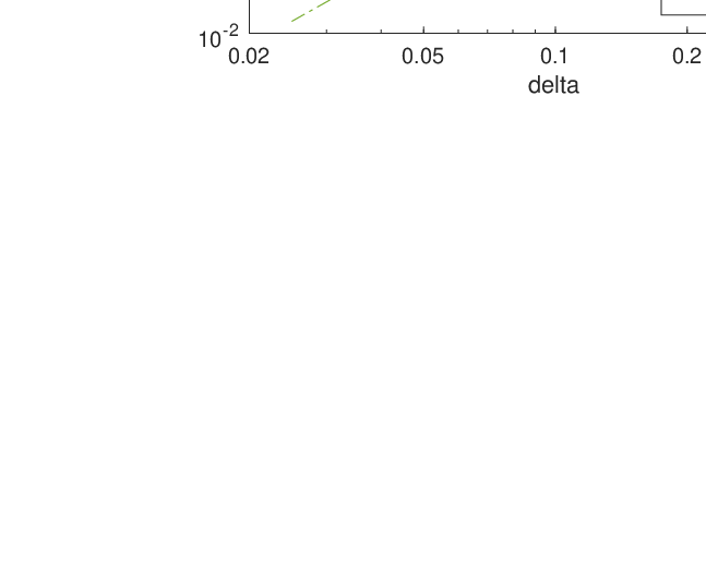
Figure 4. Comparison between the models in Examples 1.1, 1.2, and 1.3 for increasing values of ϵ\epsilon. (a) Second component u2u_{2} at time t=0.1t=0.1 for ϵ=0.25\epsilon=0.25 from model (3) (u2u_{2}), model (5) (u~2\tilde{u}_{2}), and model (6) (u^2\hat{u}_{2}). (b) Norm in W2​(QT)W_{2}(Q_{T}) of the difference between solutions of models in Examples 1.1 and 1.2, ‖u~−u‖\|\tilde{u}-u\|, and between models in Examples 1.3 and 1.1, ‖u^−u~‖\|\hat{u}-\tilde{u}\|. Norm computed using (37) as a function of ϵ\epsilon. Dash and dot-dash lines show curves O⁡(ϵ)O(\epsilon) and O⁡(ϵ2)O(\epsilon^{2}) for reference. Parameters used: N¯i=1/2\bar{N}_{i}=1/2, ε¯i=1\bar{\varepsilon}_{i}=1, D1=1.5D_{1}=1.5, D2=1D_{2}=1, V1​(x)=1−exp⁡(−120​x2)V_{1}(x)=1-\exp(-120x^{2}) and V2​(x)=0V_{2}(x)=0, d=2d=2, final time T=1T=1, J=500J=500 and M=100M=100. Initial data as in Figure 3(a).

Appendix A Proof of Lemma 2.1

Our approach is classical and the parabolic estimate mostly follows from an elliptic regularity estimate. Yet, for general cross-diffusion systems, it is well known that such elliptic results do not always hold, including for quasilinear systems with analytic dependence on uu (see for example [10] and [22]). Therefore this result needs to be proved in the case at hand. Some of the more technical arguments are detailed in well known references (for example [12, 23] concerning elliptic regularity and [8, 9, 15, 16] for the parabolic case), so we safely skip a certain number of intermediate steps, and we give the relevant references.

The following lemma provides the key regularity result.

Lemma A.1.

Given ω∈C1​(Ω¯,ℝ+)\omega\in C^{1}\left(\overline{\Omega};\mathbb{R}^{+}\right), for any u0∈H2​(Ω,ℝm)u^{0}\in H^{2}\left(\Omega;\mathbb{R}^{m}\right) and

gi∈C([0,T];H1(Ω;ℝd))∩H1(0,T;L2(Ω;ℝd)),i=1,…,mg_{i}\in C\left(\left[0,T\right];H^{1}\left(\Omega;\mathbb{R}^{d}\right)\right)\cap H^{1}\left(0,T;L^{2}\left(\Omega;\mathbb{R}^{d}\right)\right),\quad i=1,\ldots,m

the weak solution uu of

(41) ω​∂tui−∂α[Diα​β​(x,t)​∂βui+Fi​jα​(x,t)​uj+giα]=0inΩ,[Diα​β(x,t)∂βui+Fi​jα(x,t]uj+giα]⋅να=0on∂Ω,ui​(0)=ui0inΩ,\displaystyle\begin{aligned} \omega\partial_{t}u_{i}-\partial_{\alpha}\left[D_{i}^{\alpha\beta}(x,t)\partial_{\beta}u_{i}+F_{ij}^{\alpha}(x,t)u_{j}+g_{i}^{\alpha}\right]&=0&&\text{in}\quad\Omega,\\ \left[D_{i}^{\alpha\beta}(x,t)\partial_{\beta}u_{i}+F_{ij}^{\alpha}\left(x,t\right]u_{j}+g_{i}^{\alpha}\right]\cdot\nu^{\alpha}&=0&&\text{on}\quad\partial\Omega,\\ u_{i}(0)&=u_{i}^{0}&&\text{in}\quad\Omega,\end{aligned}

for i=1,…,mi=1,\ldots,m, is unique in L2​(0,T,H1​(Ω))∩C⁡([0,T],L2​(Ω))L^{2}\left(0,T;H^{1}\left(\Omega\right)\right)\cap C\left(\left[0,T\right];L^{2}\left(\Omega\right)\right) with ∂tu∈L2​(0,T,(H1​(Ω))′)\partial_{t}u\in L^{2}(0,T;(H^{1}(\Omega))^{\prime}). If the compatibility condition

(42) [Diα​β​(x,t)​∂βui0+Fi​jα​uj0+giα]⋅να=0on ​∂Ω,i=1,…,m\left[D_{i}^{\alpha\beta}(x,t)\partial_{\beta}u^{0}_{i}+F_{ij}^{\alpha}u^{0}_{j}+g_{i}^{\alpha}\right]\cdot\nu^{\alpha}=0\quad\text{on }\partial\Omega,\quad i=1,\ldots,m

holds, then uu satisfies

(43) ‖u‖W⁡(QT)≤12​CT​(‖u0‖H2​(Ω)+‖g‖C⁡([0,T],H1​(Ω))∩H1​(0,T,L2​(Ω))),\left\|u\right\|_{W\left(Q_{T}\right)}\leq\frac{1}{2}C_{T}\left(\left\|u^{0}\right\|_{H^{2}\left(\Omega\right)}+\left\|g\right\|_{C\left(\left[0,T\right];H^{1}\left(\Omega\right)\right)\cap H^{1}\left(0,T;L^{2}\left(\Omega\right)\right)}\right),

where the constant CTC_{T} is given by (68) and depends on m, λ\lambda, TT, the C1C^{1} norms of ω\omega, DD, and FF, and the domain Ω\Omega only.

Furthermore, if Fi​jα=Diα​β​∂βViF_{ij}^{\alpha}=D_{i}^{\alpha\beta}\partial_{\beta}V_{i} with Vi∈C1​(Ω¯,ℝ)V_{i}\in C^{1}\left(\overline{\Omega};\mathbb{R}\right), and for each ii, DiD_{i} and ViV_{i} do not depend on time, then

(44) ‖u‖W⁡(QT)≤12​C∞​(‖u0‖H2​(Ω)+‖g‖C⁡([0,T],H1​(Ω))∩H1​(0,T,L2​(Ω))),\left\|u\right\|_{W\left(Q_{T}\right)}\leq\frac{1}{2}C_{\infty}\left(\left\|u^{0}\right\|_{H^{2}\left(\Omega\right)}+\left\|g\right\|_{C\left(\left[0,T\right];H^{1}\left(\Omega\right)\right)\cap H^{1}\left(0,T;L^{2}\left(\Omega\right)\right)}\right),

where C∞C_{\infty}, given by (69), depends on m,λm,\lambda, the C1C^{1}norms of ω\omega, DD, FF and the domain Ω\Omega only. In particular, C∞C_{\infty} is independent of TT.

Proof.

Note that no coupling appears in (41), therefore the index ii can be dropped, as the result relates to equations, and not systems. For the purpose of this proof, it is convenient to modify the formulation of the problem to simplify the computations. We will write D=A2D=A^{2}, with A∈C1​(QT¯,ℝd×d)A\in C^{1}\left(\overline{Q_{T}};\mathbb{R}^{d\times d}\right) symmetric, positive definite and AA satisfies

(45) ‖A−1(x,t)‖∞≤λ−1/2 in QT.\left\|A^{-1}(x,t)\right\|_{\infty}\leq\lambda^{-1/2}\text{ in }Q_{T}.

We write F=A​B,F=AB, and g=A​fg=Af, so that the evolution problem under consideration can be written under the form

(46) ω∂tu−div(A2∇u+ABu+Af)=0in 𝒟′(Ω).\omega\partial_{t}u-\div\left(A^{2}\nabla u+ABu+Af\right)=0\quad\text{in }\mathcal{D}^{\prime}\left(\Omega\right).

The a priori  bounds we will use are

(47) ‖A‖L∞​(QT)+‖∇A‖L∞​(QT)\displaystyle\left\|A\right\|_{L^{\infty}\left(Q_{T}\right)}+\left\|\nabla A\right\|_{L^{\infty}\left(Q_{T}\right)} ≤MA,\displaystyle\leq M_{A},
(48) ‖B‖L∞​(QT)+‖B‖L∞​(QT)+‖∇B‖L∞​(QT)\displaystyle\left\|B\right\|_{L^{\infty}\left(Q_{T}\right)}+\left\|B\right\|_{L^{\infty}\left(Q_{T}\right)}+\left\|\nabla B\right\|_{L^{\infty}\left(Q_{T}\right)} ≤MB,\displaystyle\leq M_{B},
(49) ‖ω−1‖L∞​(QT)+‖ω‖L∞​(QT)+‖∇ω‖L∞​(QT)\displaystyle\left\|\omega^{-1}\right\|_{L^{\infty}\left(Q_{T}\right)}+\left\|\omega\right\|_{L^{\infty}\left(Q_{T}\right)}+\left\|\nabla\omega\right\|_{L^{\infty}\left(Q_{T}\right)} ≤Mω,\displaystyle\leq M_{\omega},

and

(50) ‖∂tA‖C⁡(QT¯)+‖A−1​∂tA‖C⁡(QT¯)+‖∂tA−1‖C⁡(QT¯)+‖∂t(A−1​B)‖C⁡(QT¯)≤MT.\left\|\partial_{t}A\right\|_{C\left(\overline{Q_{T}}\right)}+\left\|A^{-1}\partial_{t}A\right\|_{C\left(\overline{Q_{T}}\right)}+\left\|\partial_{t}A^{-1}\right\|_{C\left(\overline{Q_{T}}\right)}+\left\|\partial_{t}\left(A^{-1}B\right)\right\|_{C\left(\overline{Q_{T}}\right)}\leq M_{T}.

For a.e.a.e. t∈[0,T]t\in[0,T], we define 𝒜⁡(t,u,v):H1​(Ω,ℝ)×H1​(Ω,ℝ)→ℝ\mathcal{A}\left(t,u,v\right):H^{1}(\Omega;\mathbb{R})\times H^{1}(\Omega;\mathbb{R})\to\mathbb{R} by

(51) 𝒜⁡(t,u,v)=∫Ω(A2)α​β​(t,x)​∂βu​∂αv​𝑑x+∫Ω(A​B)α​(t,x)​u​∂αv​𝑑x.\mathcal{A}(t,u,v)=\int_{\Omega}\left(A^{2}\right)^{\alpha\beta}\left(t,x\right)\partial_{\beta}u\partial_{\alpha}v\,\mathrm{d}x+\int_{\Omega}\left(AB\right)^{\alpha}\left(t,x\right)u\partial_{\alpha}v\,\mathrm{d}x.

Using the a priori  bounds (47) and (48), we find the upper bound

𝒜⁡(t,u,v)≤MA​(MA+MB)​‖u‖H1​(Ω)​‖v‖H1​(Ω).\mathcal{A}(t,u,v)\leq M_{A}\left(M_{A}+M_{B}\right)\|u\|_{H^{1}(\Omega)}\|v\|_{H^{1}(\Omega)}.

Furthermore, using (45) as well, we have the lower bound

(52) 𝒜⁡(t,u,v)≥λ​‖u‖H1​(Ω)2−MA​MB​‖u‖L2​(Ω)​‖u‖H1​(Ω)≥12​λ​‖u‖H1​(Ω)2−12​λ​MA2​MB2​‖u‖L2​(Ω)2.\mathcal{A}(t,u,v)\geq\lambda\|u\|_{H^{1}(\Omega)}^{2}-M_{A}M_{B}\|u\|_{L^{2}(\Omega)}\|u\|_{H^{1}(\Omega)}\geq\frac{1}{2}\lambda\|u\|_{H^{1}(\Omega)}^{2}-\frac{1}{2\lambda}M_{A}^{2}M_{B}^{2}\|u\|_{L^{2}(\Omega)}^{2}.

We may therefore apply the parabolic version of the Lax–Milgram Theorem of Lions [1, 16] to deduce that there exists a unique solution of (41) u∈L2​(0,T,H1​(Ω,ℝ))∩C⁡([0,T],L2​(Ω,ℝ))u\in L^{2}(0,T;H^{1}(\Omega;\mathbb{R}))\cap C([0,T];L^{2}(\Omega;\mathbb{R})) with ∂tu∈L2​(0,T,H1​(Ω,ℝ)′)\partial_{t}u\in L^{2}(0,T;H^{1}(\Omega;\mathbb{R})^{\prime}).

We now derive an explicit bound. Integrating (46) by parts against uu we find

∂t12∫Ωωu2dx+∫ΩA2(x,t)∇u⋅∇udx+∫ΩuAB⋅∇udx+∫ΩAf⋅∇udx=0.\partial_{t}\frac{1}{2}\int_{\Omega}\omega u^{2}\,\mathrm{d}x+\int_{\Omega}A^{2}(x,t)\nabla u\cdot\nabla u\,\mathrm{d}x+\int_{\Omega}uAB\cdot\nabla u\,\mathrm{d}x+\int_{\Omega}Af\cdot\nabla u\,\mathrm{d}x=0.

Thus, using (52) and Cauchy–Schwarz

∂t(12‖ωu‖L2​(Ω)2)+12∥A∇u∥H1​(Ω)2≤‖f‖L2​(Ω)2+‖ω−12B‖L∞​(Ω)2‖ωu‖L2​(Ω)2,\partial_{t}\left(\frac{1}{2}\left\|\sqrt{\omega}u\right\|_{L^{2}\left(\Omega\right)}^{2}\right)+\frac{1}{2}\|A\nabla u\|_{H^{1}(\Omega)}^{2}\leq\left\|f\right\|_{L^{2}\left(\Omega\right)}^{2}+\left\|\omega^{-\frac{1}{2}}B\right\|_{L^{\infty}(\Omega)}^{2}\left\|\sqrt{\omega}u\right\|_{L^{2}\left(\Omega\right)}^{2},

which leads to two bounds

(53) ‖u‖C⁡([0,T],L2​(Ω))≤Mω12​(exp⁡(2​Mω​MB​T)​‖f‖L2​(QT)+Mω12​‖u0‖L2​(Ω)),\left\|u\right\|_{C\left(\left[0,T\right],L^{2}\left(\Omega\right)\right)}\leq M_{\omega}^{\frac{1}{2}}\left(\exp\left(\sqrt{2}M_{\omega}M_{B}T\right)\left\|f\right\|_{L^{2}\left(Q_{T}\right)}+M_{\omega}^{\frac{1}{2}}\left\|u^{0}\right\|_{L^{2}\left(\Omega\right)}\right),

and

(54) λ/2∥∇u∥L2​(0,T,L2​(Ω))≤1/2∥A∇u∥L2​(0,T,L2​(Ω))≤Mω2‖u0‖L2​(Ω)+‖f‖L2​(QT).\sqrt{\lambda/2}\|\nabla u\|_{L^{2}\left(0,T;L^{2}(\Omega)\right)}\leq\sqrt{1/2}\|A\nabla u\|_{L^{2}\left(0,T;L^{2}(\Omega)\right)}\leq\sqrt{\frac{M_{\omega}}{2}}\left\|u^{0}\right\|_{L^{2}\left(\Omega\right)}+\left\|f\right\|_{L^{2}\left(Q_{T}\right)}.

Note that ∫Ωu​𝑑x=∫Ωu0​𝑑x\int_{\Omega}u\,\mathrm{d}x=\int_{\Omega}u^{0}\,\mathrm{d}x for all times. As a result,

‖u‖L2​(0,T,H1​(Ω))\displaystyle\left\|u\right\|_{L^{2}\left(0,T;H^{1}(\Omega)\right)} ≤T​|1|Ω|​∫Ωu0​𝑑x|+‖u−1|Ω|​∫Ωu​𝑑x‖L2​(0,T,L2​(Ω))+‖∇u‖L2​(0,T,L2​(Ω))\displaystyle\leq\sqrt{T}\left|\frac{1}{\left|\Omega\right|}\int_{\Omega}u^{0}\,\mathrm{d}x\right|+\left\|u-\frac{1}{\left|\Omega\right|}\int_{\Omega}u\,\mathrm{d}x\right\|_{L^{2}\left(0,T;L^{2}(\Omega)\right)}+\left\|\nabla u\right\|_{L^{2}\left(0,T;L^{2}(\Omega)\right)}
≤T|1|Ω|∫Ωu0dx|+(CP(Ω)+1)λ−1/2‖A∇u‖L2​(0,T,L2​(Ω))\displaystyle\leq\sqrt{T}\left|\frac{1}{\left|\Omega\right|}\int_{\Omega}u^{0}\,\mathrm{d}x\right|+(C_{P}\left(\Omega\right)+1)\lambda^{-1/2}\left\|A\nabla u\right\|_{L^{2}\left(0,T;L^{2}(\Omega)\right)}
(55) ≤C1​(‖u0‖L2​(Ω)+‖f‖L2​(QT)),\displaystyle\leq C_{1}\left(\left\|u^{0}\right\|_{L^{2}\left(\Omega\right)}+\left\|f\right\|_{L^{2}\left(Q_{T}\right)}\right),

where CP​(Ω)C_{P}(\Omega) is the Poincaré–Wirtinger constant, and

(56) C1=T|Ω|−1/2+(CP(Ω)+1)Mω2​λ.C_{1}=\sqrt{T}\left|\Omega\right|^{-1/2}+(C_{P}\left(\Omega\right)+1)\sqrt{\frac{M_{\omega}}{2\lambda}}.

Let us now focus on higher regularity. We are going to show that

u∈C⁡([0,T],H2​(Ω))∩H1​(0,T,H1​(Ω)).u\in C\left([0,T];H^{2}(\Omega)\right)\cap H^{1}\left(0,T;H^{1}(\Omega)\right).

We write

(57) Φ=A∇u+Bu+f.\Phi=A\nabla u+Bu+f.

Thanks to (54) and (55), we have

‖Φ‖L2​(0,T,L2​(Ω))≤C2​(‖u0‖L2​(Ω)+‖f‖L2​(QT)),\|\Phi\|_{L^{2}\left(0,T;L^{2}(\Omega)\right)}\leq C_{2}\left(\left\|u^{0}\right\|_{L^{2}\left(\Omega\right)}+\left\|f\right\|_{L^{2}\left(Q_{T}\right)}\right),

with

(58) C2=1+Mω+MB​C1.C_{2}=1+\sqrt{M_{\omega}}+M_{B}C_{1}.

Next, we are going to test (41) against η=∂tu−ω−1​div⁡(A​Φ)\eta=\partial_{t}u-\omega^{-1}\div\left(A\Phi\right). Notice that we have to ensure that η\eta is a valid test function. We just sketch the procedure, namely we consider ητ,h=Δτ​u−ω−1​Δhα​(Aα​β​Φβ)\eta_{\tau,h}=\Delta_{\tau}u-\omega^{-1}\Delta_{h}^{\alpha}\left(A^{\alpha\beta}\Phi^{\beta}\right), where the difference quotient time derivative is given by Δτu=(u(⋅+τ)−u(⋅))τ−1\Delta_{\tau}u=\left(u\left(\cdot+\tau\right)-u\left(\cdot\right)\right)\tau^{-1} and difference quotient space derivatives in direction ii is given by Δ−hαψ=(ψ(⋅+heα)−ψ(⋅))h−1\Delta_{-h}^{\alpha}\psi=\left(\psi\left(\cdot+h\text{e}_{\alpha}\right)-\psi\left(\cdot\right)\right)h^{-1}. We have to test (41) against ητ,h\eta_{\tau,h} and subsequently pass to the limit for τ,h→0\tau,h\to 0, paying attention to the direction normal to the boundary near ∂Ω\partial\Omega. This step is somewhat technical but straightforward and it justifies the following calculations rigorously. To simplify the exposition, we use directly ∂tu−ω−1​div⁡(A​Φ)\partial_{t}u-\omega^{-1}\div\left(A\Phi\right) as the test function in the following steps, and obtain

(59) ∫Ωω​(∂tu)2​𝑑x+∫Ω(A​Φ)⋅∇(−ω−1​div⁡(A​Φ))​𝑑x−2​∫Ω∂tu​div⁡(A​Φ)​𝑑x=0\int_{\Omega}\omega\left(\partial_{t}u\right)^{2}\,\mathrm{d}x+\int_{\Omega}\left(A\Phi\right)\cdot\nabla\left(-\omega^{-1}\div\left(A\Phi\right)\right)\,\mathrm{d}x-2\int_{\Omega}\partial_{t}u\div(A\Phi)\,\mathrm{d}x=0

As A​Φ⋅ν=0A\Phi\cdot\nu=0, we find that

(60) ∫Ω(A​Φ)⋅∇(−ω−1​div⁡(A​Φ))​𝑑x=∫Ωω−1​(div⁡(A​Φ))2​𝑑x.\int_{\Omega}\left(A\Phi\right)\cdot\nabla\left(-\omega^{-1}\div\left(A\Phi\right)\right)\,\mathrm{d}x=\int_{\Omega}\omega^{-1}\left(\div\left(A\Phi\right)\right)^{2}\,\mathrm{d}x.

Let us now turn to the mixed term. We have

(61) −2∫Ω∂tudiv(AΦ)dx\displaystyle-2\int_{\Omega}\partial_{t}u\div(A\Phi)\,\mathrm{d}x =2∫Ω∂t((A−1A)∇u)⋅(AΦ)dx=2∫Ω[∂t(A∇u)+A∂t(A−1)A∇u]⋅Φdx\displaystyle=2\int_{\Omega}\partial_{t}\left(\left(A^{-1}A\right)\nabla u\right)\cdot\left(A\Phi\right)\,\mathrm{d}x=2\int_{\Omega}\left[\partial_{t}(A\nabla u)+A\partial_{t}(A^{-1})A\nabla u\right]\cdot\Phi\,\mathrm{d}x
=2​∫Ω[∂t(Φ)+A​∂t(A−1)​Φ]⋅Φ​𝑑x−2​∫Ω[∂t(B​u+f)+A​∂t(A−1)​(B​u+f)]⋅Φ​𝑑x.\displaystyle=2\int_{\Omega}\left[\partial_{t}(\Phi)+A\partial_{t}(A^{-1})\Phi\right]\cdot\Phi\,\mathrm{d}x-2\int_{\Omega}\left[\partial_{t}(Bu+f)+A\partial_{t}(A^{-1})(Bu+f)\right]\cdot\Phi\,\mathrm{d}x.

Inserting (60) and (61) into (59) and using Cauchy–Schwarz, we obtain

‖ω​∂tu‖L2​(Ω)2\displaystyle\left\|\sqrt{\omega}\partial_{t}u\right\|_{L^{2}(\Omega)}^{2} +∫Ωω−1div(AΦ)2dx+∂t‖Φ‖L2​(Ω)2\displaystyle+\int_{\Omega}\omega^{-1}\div\left(A\Phi\right)^{2}\,\mathrm{d}x+\partial_{t}\left\|\Phi\right\|_{L^{2}\left(\Omega\right)}^{2}
(62) ≤2​MT​MA​(‖Φ‖L2​(Ω)2+‖f‖L2​(Ω)​‖Φ‖L2​(Ω))+2​‖∂tf‖L2​(Ω)​‖Φ‖L2​(Ω)\displaystyle\leq 2M_{T}M_{A}\left(\left\|\Phi\right\|_{L^{2}\left(\Omega\right)}^{2}+\left\|f\right\|_{L^{2}\left(\Omega\right)}\left\|\Phi\right\|_{L^{2}\left(\Omega\right)}\right)+2\left\|\partial_{t}f\right\|_{L^{2}\left(\Omega\right)}\left\|\Phi\right\|_{L^{2}\left(\Omega\right)}
+2​MT​MA​MB​‖u‖L2​(Ω)​‖Φ‖L2​(Ω)+2​MB​Mω12​‖ω​∂tu‖L2​(Ω)​‖Φ‖L2​(Ω).\displaystyle\quad+2M_{T}M_{A}M_{B}\left\|u\right\|_{L^{2}\left(\Omega\right)}\left\|\Phi\right\|_{L^{2}\left(\Omega\right)}+2M_{B}M_{\omega}^{\frac{1}{2}}\left\|\sqrt{\omega}\partial_{t}u\right\|_{L^{2}\left(\Omega\right)}\left\|\Phi\right\|_{L^{2}\left(\Omega\right)}.

Using Young’s inequality, we recombine inequality (62) to find

12​‖ω​∂tu‖L2​(Ω)2+‖ω​div⁡(A​Φ)‖L2​(Ω)2+∂t‖Φ‖L2​(Ω)2≤(2​C3+1)​‖Φ‖L2​(Ω)2+MB2​‖u‖L2​(Ω)2+‖∂tf‖L2​(Ω)2+‖f‖L2​(Ω)\frac{1}{2}\left\|\sqrt{\omega}\partial_{t}u\right\|_{L^{2}\left(\Omega\right)}^{2}+\left\|\sqrt{\omega}\div\left(A\Phi\right)\right\|_{L^{2}\left(\Omega\right)}^{2}+\partial_{t}\left\|\Phi\right\|_{L^{2}\left(\Omega\right)}^{2}\leq\left(2C_{3}+1\right)\left\|\Phi\right\|_{L^{2}\left(\Omega\right)}^{2}+M_{B}^{2}\left\|u\right\|_{L^{2}\left(\Omega\right)}^{2}+\left\|\partial_{t}f\right\|_{L^{2}\left(\Omega\right)}^{2}+\left\|f\right\|_{L^{2}\left(\Omega\right)}

with

C3=2​MT​MA​(1+2​MT​MA)+2​MB2​Mω.C_{3}=2M_{T}M_{A}\left(1+2M_{T}M_{A}\right)+2M_{B}^{2}M_{\omega}.

Integrating in time, we find

‖Φ‖C⁡([0,T],L2​(Ω))2\displaystyle\left\|\Phi\right\|_{C\left(\left[0,T\right],L^{2}\left(\Omega\right)\right)}^{2} +12​‖ω​∂tu‖L2​(QT)2+‖ω​div⁡(A​Φ)‖L2​(QT)2\displaystyle+\frac{1}{2}\left\|\sqrt{\omega}\partial_{t}u\right\|_{L^{2}\left(Q_{T}\right)}^{2}+\left\|\sqrt{\omega}\div\left(A\Phi\right)\right\|_{L^{2}\left(Q_{T}\right)}^{2}
≤C4​(‖u0‖L2​(Ω)+‖f‖L2​(QT))2\displaystyle\leq C_{4}\left(\left\|u^{0}\right\|_{L^{2}\left(\Omega\right)}+\left\|f\right\|_{L^{2}\left(Q_{T}\right)}\right)^{2}
+‖A∇u0+Bu0+f(t=0)‖L2​(Ω)2+‖∂tf‖L2​(QT)2+‖f‖L2​(QT)2,\displaystyle\quad+\left\|A\nabla u^{0}+Bu^{0}+f\left(t=0\right)\right\|_{L^{2}(\Omega)}^{2}+\left\|\partial_{t}f\right\|_{L^{2}\left(Q_{T}\right)}^{2}+\left\|f\right\|_{L^{2}\left(Q_{T}\right)}^{2},

with

(63) C4=(2​C3+1)​C22+MB2​C12.C_{4}=\left(2C_{3}+1\right)C_{2}^{2}+M_{B}^{2}C_{1}^{2}.

Let us now check that this allows us to define ∂tu|t=0\left.\partial_{t}u\right|_{t=0} in an appropriate sense. Since

‖∇u‖C⁡([0,T],L2​(Ω))≤λ−12​(‖Φ‖C⁡([0,T],L2​(Ω))+MB​‖u‖C⁡([0,T],L2​(Ω))+‖f‖C⁡([0,T],L2​(Ω))),\left\|\nabla u\right\|_{C\left(\left[0,T\right],L^{2}\left(\Omega\right)\right)}\leq\lambda^{-\frac{1}{2}}\left(\left\|\Phi\right\|_{C\left(\left[0,T\right],L^{2}\left(\Omega\right)\right)}+M_{B}\left\|u\right\|_{C\left(\left[0,T\right],L^{2}\left(\Omega\right)\right)}+\left\|f\right\|_{C\left(\left[0,T\right],L^{2}\left(\Omega\right)\right)}\right),

for any v∈H1​(Ω)v\in H^{1}\left(\Omega\right), the map

t→∫Ω[A(x,t)∇u⋅∇v+Bu⋅∇v+fu⋅∇v]dxt\to\int_{\Omega}\left[A(x,t)\nabla u\cdot\nabla v+Bu\cdot\nabla v+fu\cdot\nabla v\right]\,\text{d}x

is continuous on [0,T][0,T]. In other words, we define ∂tu|t=0∈(H1​(Ω))′\left.\partial_{t}u\right|_{t=0}\in\left(H^{1}(\Omega)\right)^{\prime} as follows

∫Ω∂tu|t=0​v​d​x\displaystyle\int_{\Omega}\left.\partial_{t}u\right|_{t=0}v\,\text{d}x =limt↓0∫Ω[A(x,t)∇u⋅∇v+B(x,t)u.∇v+f(x,0)⋅∇v]dx\displaystyle=\lim_{t\downarrow 0}\int_{\Omega}\left[A(x,t)\nabla u\cdot\nabla v+B(x,t)u.\nabla v+f(x,0)\cdot\nabla v\right]\text{d}x
=∫Ω[A(x,0)∇u0⋅∇v+B(x,0)u0.∇v+f(x,0)⋅∇v]dx,\displaystyle=\int_{\Omega}\left[A(x,0)\nabla u^{0}\cdot\nabla v+B(x,0)u^{0}.\nabla v+f(x,0)\cdot\nabla v\right]\text{d}x,

provided that the compatibility condition (42) holds, that is,

[A(x,0)∇u0−B(x,0)u0−f(x,0)]⋅ν=0.\left[A(x,0)\nabla u^{0}-B(x,0)u^{0}-f(x,0)\right]\cdot\nu=0.

An integration by parts then shows that

∫Ω∂tu|t=0vdx=∫Ωdiv[A(x,0)∇u0+B(x,0)u0+f(x,0)]vdx,\int_{\Omega}\left.\partial_{t}u\right|_{t=0}v\,\text{d}x=\int_{\Omega}\div\left[A(x,0)\nabla u^{0}+B(x,0)u^{0}+f(x,0)\right]v\,\text{d}x,

which, in turn, shows that ∂tu|t=0∈L2​(Ω)\left.\partial_{t}u\right|_{t=0}\in L^{2}(\Omega) and

(64) ‖∂tu|t=0‖L2​(Ω)≤(MA+MB)​(‖u0‖H2​(Ω)+‖f‖C⁡([0,T],H1​(Ω))).\left\|\left.\partial_{t}u\right|_{t=0}\right\|_{L^{2}\left(\Omega\right)}\leq\left(M_{A}+M_{B}\right)\left(\left\|u^{0}\right\|_{H^{2}\left(\Omega\right)}+\left\|f\right\|_{C\left(\left[0,T\right];H^{1}\left(\Omega\right)\right)}\right).

We now notice that ∂tu\partial_{t}u is a weak solution of (41), where ff is replaced by ∂tf+∂tA∇u+∂tBu\partial_{t}f+\partial_{t}A\nabla u+\partial_{t}Bu and u0u^{0} is replaced by ∂tu|t=0\left.\partial_{t}u\right|_{t=0}. From (55) we obtain

(65) ‖∂tf+∂tA∇u+∂tBu‖L2​(QT)≤max(MTC1,1)(‖u0‖L2​(Ω)+‖f‖H1​(0,T,L2​(Ω)))\left\|\partial_{t}f+\partial_{t}A\nabla u+\partial_{t}Bu\right\|_{L^{2}\left(Q_{T}\right)}\leq\max(M_{T}C_{1},1)\left(\left\|u^{0}\right\|_{L^{2}\left(\Omega\right)}+\left\|f\right\|_{H^{1}\left(0,T;L^{2}(\Omega)\right)}\right)

Thus (54) becomes

λ2​‖∂t∇u‖L2​((0,T),L2​(Ω))\displaystyle\sqrt{\frac{\lambda}{2}}\left\|\partial_{t}\nabla u\right\|_{L^{2}\left(\left(0,T\right);L^{2}\left(\Omega\right)\right)} ≤Mω2‖∂tu|t=0‖L2​(Ω)+‖∂tf+∂tA∇u+∂tBu‖L2​(QT)\displaystyle\leq\sqrt{\frac{M_{\omega}}{2}}\left\|\left.\partial_{t}u\right|_{t=0}\right\|_{L^{2}\left(\Omega\right)}+\left\|\partial_{t}f+\partial_{t}A\nabla u+\partial_{t}Bu\right\|_{L^{2}\left(Q_{T}\right)}
≤Mω2​(MA+MB)​(‖u0‖H2​(Ω)+‖f‖C⁡([0,T],H1​(Ω)))\displaystyle\leq\sqrt{\frac{M_{\omega}}{2}}(M_{A}+M_{B})\left(\left\|u^{0}\right\|_{H^{2}\left(\Omega\right)}+\left\|f\right\|_{C\left(\left[0,T\right];H^{1}\left(\Omega\right)\right)}\right)
+max⁡(MT​C1,1)​(‖u0‖L2​(Ω)+‖f‖H1​(0,T,L2​(Ω))),\displaystyle\quad+\max(M_{T}C_{1},1)\left(\left\|u^{0}\right\|_{L^{2}\left(\Omega\right)}+\left\|f\right\|_{H^{1}\left(0,T;L^{2}(\Omega)\right)}\right),

and (53) gives

‖∂tu‖C⁡([0,T],L2​(Ω))\displaystyle\left\|\partial_{t}u\right\|_{C\left([0,T];L^{2}\left(\Omega\right)\right)} ≤Mω12[exp(2MωMBT)‖∂tf+∂tA∇u+∂tBu‖L2​(QT)+Mω12‖∂tu|t=0‖L2​(Ω)]\displaystyle\leq M_{\omega}^{\frac{1}{2}}\left[\exp\left(\sqrt{2}M_{\omega}M_{B}T\right)\left\|\partial_{t}f+\partial_{t}A\nabla u+\partial_{t}Bu\right\|_{L^{2}\left(Q_{T}\right)}+M_{\omega}^{\frac{1}{2}}\left\|\left.\partial_{t}u\right|_{t=0}\right\|_{L^{2}\left(\Omega\right)}\right]
≤C5​(‖u0‖H2​(Ω)+‖f‖C⁡([0,T],H1​(Ω))+‖f‖H1​(0,T,L2​(Ω))),\displaystyle\leq C_{5}\left(\left\|u^{0}\right\|_{H^{2}\left(\Omega\right)}+\left\|f\right\|_{C\left(\left[0,T\right];H^{1}\left(\Omega\right)\right)}+\left\|f\right\|_{H^{1}\left(0,T;L^{2}\left(\Omega\right)\right)}\right),

with

(66) C5=Mω​(MA+MB)+Mω12​max⁡(MT​C1,1)​exp⁡(2​Mω​MB​T).C_{5}=M_{\omega}\left(M_{A}+M_{B}\right)+M_{\omega}^{\frac{1}{2}}\max(M_{T}C_{1},1)\exp\left(\sqrt{2}M_{\omega}M_{B}T\right).

Finally, we observe that the right-hand side of the identity

div(A∇u)=∂tu−div(Bu+f),\div\left(A\nabla u\right)=\partial_{t}u-\div\left(Bu+f\right),

belongs to C⁡([0,T],L2​(Ω))C\left([0,T];L^{2}\left(\Omega\right)\right), and therefore the left-hand side belongs to the same space. This in turn shows that u∈H2​(Ω)u\in H^{2}(\Omega) for any tt, in fact u∈C⁡([0,T],H2​(Ω))u\in C\left(\left[0,T\right];H^{2}\left(\Omega\right)\right), see, for example, [19], with

‖u‖C⁡([0,T],H2​(Ω))≤C⁡(Ω,MA,λ)​(C5+MB​C1)​(‖u0‖H2​(Ω)+‖f‖C⁡([0,T],H1​(Ω))+‖f‖H1​(0,T,L2​(Ω))).\left\|u\right\|_{C\left(\left[0,T\right];H^{2}\left(\Omega\right)\right)}\leq C(\Omega,M_{A},\lambda)\left(C_{5}+M_{B}C_{1}\right)\left(\left\|u^{0}\right\|_{H^{2}\left(\Omega\right)}+\left\|f\right\|_{C\left(\left[0,T\right];H^{1}\left(\Omega\right)\right)}+\left\|f\right\|_{H^{1}\left(0,T;L^{2}\left(\Omega\right)\right)}\right).

Altogether, we have shown

(67) ‖u‖C⁡([0,T],H2​(Ω))+‖u‖H1​(0,T,H1​(Ω))≤12​CT​(‖u0‖H2​(Ω)+‖f‖C⁡([0,T],H1​(Ω))+‖f‖H1​(0,T,L2​(Ω))),\left\|u\right\|_{C\left(\left[0,T\right];H^{2}\left(\Omega\right)\right)}+\left\|u\right\|_{H^{1}\left(0,T;H^{1}\left(\Omega\right)\right)}\leq\frac{1}{2}C_{T}\left(\left\|u^{0}\right\|_{H^{2}\left(\Omega\right)}+\left\|f\right\|_{C\left(\left[0,T\right];H^{1}\left(\Omega\right)\right)}+\left\|f\right\|_{H^{1}\left(0,T;L^{2}\left(\Omega\right)\right)}\right),

where

(68) CT=2​(C⁡(Ω,MA,λ)​(C5+MB​C1)+Mωλ​(MA+MB)+2λ​max⁡(MT​C1,1)),C_{T}=2\left(C(\Omega,M_{A},\lambda)\left(C_{5}+M_{B}C_{1}\right)+\sqrt{\frac{M_{\omega}}{\lambda}}\left(M_{A}+M_{B}\right)+\sqrt{\frac{2}{\lambda}}\max(M_{T}C_{1},1)\right),

and C4C_{4} and C5C_{5} are given by (63) and (66), respectively, as announced.

Let us now turn to the particular case when B=A∇VB=A\nabla V, with V∈C2​(Ω¯)V\in C^{2}\left(\overline{\Omega}\right), and AA and VV are independent of time. We perform the change of unknown w=u​exp⁡Vw=u\exp V and, thanks to Lemma A.3, we can study the problem satisfied by ww. We have

exp(−V)∂tw−div[Aexp(−V)∇w+f]\displaystyle\exp\left(-V\right)\partial_{t}w-\div\left[A\exp\left(-V\right)\nabla w+f\right] =0\displaystyle=0 inΩ,\displaystyle\text{in}\quad\Omega,
[Aexp(−V)∇w+f]⋅ν\displaystyle\left[A\exp(-V)\nabla w+f\right]\cdot\nu =0\displaystyle=0 on∂Ω,\displaystyle\text{on}\quad\partial\Omega,
w⁡(0)\displaystyle w(0) =u0​exp⁡(V)\displaystyle=u^{0}\exp(V) inΩ,\displaystyle\text{in}\quad\Omega,

that is, the same system as (41) above, with ω=exp⁡(−V)\omega=\exp(-V), MB=0M_{B}=0 and MT=0.M_{T}=0. In this case,

C2=1+Mω,C3=0,C4=C22,C5=Mω​MA+Mω12,C_{2}=1+\sqrt{M_{\omega}},\quad C_{3}=0,\quad C_{4}=C_{2}^{2},\quad C_{5}=M_{\omega}M_{A}+M_{\omega}^{\frac{1}{2}},

and the constant CTC_{T} in (68) becomes

C~′=2​(C⁡(Ω,MA,λ)​C5+Mωλ​MA+2λ),\tilde{C}^{\prime}=2\left(C(\Omega,M_{A},\lambda)C_{5}+\sqrt{\frac{M_{\omega}}{\lambda}}M_{A}+\sqrt{\frac{2}{\lambda}}\right),

and it does not depend on TT. Thanks to Lemma A.3, we find that in terms of uu the bound (67) holds with the following constant

(69) C∞=C~​[(1+MV′)2+MV′′]​exp⁡MV,C_{\infty}=\tilde{C}\left[\left(1+M_{V}^{\prime}\right)^{2}+M_{V}^{\prime\prime}\right]\exp M_{V},

which again is independent of TT. ∎

Remark A.2 (Ellipticity bound for ϵ\epsilon).

Suppose that an a priori bound for uu on QTQ_{T} is known, say u∗=supQT|u|u^{*}=\sup_{Q_{T}}|u|. For any ξiα∈ℝd×m,ζj∈ℝm\xi_{i}^{\alpha}\in\mathbb{R}^{d\times m},\zeta_{j}\in\mathbb{R}^{m}, we have the lower bound

(70) 𝔇i​jα​β​(t,x,y)​ξiα​ξjβ=Diα​β​(t,x)​ξiα​ξiβ+ϵ​ai​jα​β​(t,x)​ϕi​jα​β​(y)​ξiα​ξjβ≥(λ−ϵ​L0​(u∗)​‖a‖∞)​|ξ|2,\displaystyle\begin{aligned} \mathfrak{D}_{ij}^{\alpha\beta}(t,x,y)\xi_{i}^{\alpha}\xi_{j}^{\beta}=D_{i}^{\alpha\beta}(t,x)\xi_{i}^{\alpha}\xi_{i}^{\beta}+\epsilon a_{ij}^{\alpha\beta}(t,x)\phi_{ij}^{\alpha\beta}(y)\xi_{i}^{\alpha}\xi_{j}^{\beta}\geq(\lambda-\epsilon L_{0}(u^{*})\|a\|_{\infty})|\xi|^{2},\end{aligned}

where ‖a‖∞=maxi,j,α,β,x⁡|ai​jα​β​(x)|\|a\|_{\infty}=\max_{i,j,\alpha,\beta,x}|a_{ij}^{\alpha\beta}(x)| and L0L_{0} is given in (16). Therefore, choosing

(71) ϵ<min⁡(λ1+‖a‖∞​L0​(u∗),1)\epsilon<\min\left(\frac{\lambda}{1+\|a\|_{\infty}L_{0}(u^{*})},1\right)

guarantees coercivity, and this is sufficient to ensure existence and uniqueness of weak solutions of (28), and consequently of (9) via Lax–Milgram lemma. We use relation (71) to derive an a priori upper bound for ϵ\epsilon in a specific case, see Lemma 3.1.

Lemma A.3.

Given V∈C2​(Ω¯)V\in C^{2}\left(\overline{\Omega}\right), the map u→u​exp⁡(V)u\to u\exp(V) is a bi-continuous isomorphism in C⁡([0,T],H2​(Ω))∩H1​(0,T,H1​(Ω)).C\left(\left[0,T\right];H^{2}\left(\Omega\right)\right)\cap H^{1}\left(0,T;H^{1}\left(\Omega\right)\right). The following inequalities hold

‖u​exp⁡(V)‖W⁡(0,T,Ω)\displaystyle\left\|u\exp(V)\right\|_{W\left(0,T,\Omega\right)} ≤[(1+MV′)2+MV′′]​exp⁡MV​‖u‖W⁡(0,T,Ω),\displaystyle\leq\left[\left(1+M_{V}^{\prime}\right)^{2}+M_{V}^{\prime\prime}\right]\exp M_{V}\left\|u\right\|_{W\left(0,T,\Omega\right)},
‖u‖W⁡(0,T,Ω)\displaystyle\left\|u\right\|_{W\left(0,T,\Omega\right)} ≤[(1+MV′)2+MV′′]​exp⁡MV​‖u​exp⁡(V)‖W⁡(0,T,Ω),\displaystyle\leq\left[\left(1+M_{V}^{\prime}\right)^{2}+M_{V}^{\prime\prime}\right]\exp M_{V}\left\|u\exp(V)\right\|_{W\left(0,T,\Omega\right)},

where MV=supΩ|V|M_{V}=\sup_{\Omega}\left|V\right|, MV′=supΩ|∇V|M_{V}^{\prime}=\sup_{\Omega}\left|\nabla V\right| and MV′′=supΩ|∇2V|.M_{V}^{\prime\prime}=\sup_{\Omega}\left|\nabla^{2}V\right|.

Proof.

Note that it is sufficient to prove one inequality, as replacing VV by −V-V changes the map to its inverse. Indeed, we have

‖u​exp⁡(V)‖L2​(Ω)\displaystyle\left\|u\exp(V)\right\|_{L^{2}(\Omega)} ≤exp⁡MV​‖u‖L2​(Ω),\displaystyle\leq\exp M_{V}\left\|u\right\|_{L^{2}(\Omega)},
‖u​exp⁡(V)‖H1​(Ω)\displaystyle\left\|u\exp(V)\right\|_{H^{1}(\Omega)} ≤(1+MV′)​exp⁡MV​‖u‖H1​(Ω),\displaystyle\leq\left(1+M_{V}^{\prime}\right)\exp M_{V}\left\|u\right\|_{H^{1}(\Omega)},
‖u​exp⁡(V)‖H2​(Ω)\displaystyle\left\|u\exp(V)\right\|_{H^{2}(\Omega)} ≤[(1+MV′)2+MV′′]​exp⁡MV​‖u‖H2​(Ω).\displaystyle\leq\left[\left(1+M_{V}^{\prime}\right)^{2}+M_{V}^{\prime\prime}\right]\exp M_{V}\left\|u\right\|_{H^{2}(\Omega)}.

∎

The second step in the proof of Lemma 2.1 concerns the regularity of the forcing term ff, which coincides with the regularity of the cross-diffusion term, provided that hh and uu are in W⁡(QT)W\left(Q_{T}\right).

Lemma A.4.

The map

(72) P:QT×C∞​(QT,ℝm)2→C2​(QT:ℝm×d)(t,x,h,u)→ai​jα​β​(t,x)​ϕi​jα​β​(h)​∂βuj+bi​jα​(t,x)​ψi​jα​(h)​uj,\displaystyle\begin{aligned} P:Q_{T}\times C^{\infty}\left(Q_{T};\mathbb{R}^{m}\right)^{2}\quad&\to\quad C^{2}\left(Q_{T}:\mathbb{R}^{m\times d}\right)\\ \left(t,x,h,u\right)\quad&\to\quad a_{ij}^{\alpha\beta}(t,x)\phi_{ij}^{\alpha\beta}\left(h\right)\partial_{\beta}u_{j}+b_{ij}^{\alpha}(t,x)\psi_{ij}^{\alpha}\left(h\right)u_{j},\end{aligned}

has the following property

P⁡(QT×W⁡(QT)×W⁡(QT))⊂C⁡([0,T],H1​(Ω,ℝm))∩H1​(0,T,L2​(Ω,ℝm)).P\left(Q_{T}\times W\left(Q_{T}\right)\times W\left(Q_{T}\right)\right)\subset C\left(\left[0,T\right];H^{1}\left(\Omega;\mathbb{R}^{m}\right)\right)\cap H^{1}\left(0,T;L^{2}\left(\Omega;\mathbb{R}^{m}\right)\right).

Furthermore, there holds

sup[0,T](‖∇Pi​(t,x,h,u)‖L2​(Ω)+‖Pi​(t,x,h,u)‖L2​(Ω))+‖∂tPi​(t,x,h,u)‖L2​(QT)≤K0​(‖h‖W⁡(QT))​‖u‖W⁡(QT),\sup_{\left[0,T\right]}\left(\left\|\nabla P_{i}(t,x,h,u)\right\|_{L^{2}(\Omega)}+\left\|P_{i}\left(t,x,h,u\right)\right\|_{L^{2}\left(\Omega\right)}\right)+\left\|\partial_{t}P_{i}\left(t,x,h,u\right)\right\|_{L^{2}\left(Q_{T}\right)}\leq K_{0}\left(\left\|h\right\|_{W\left(Q_{T}\right)}\right)\left\|u\right\|_{W\left(Q_{T}\right)},

where K0K_{0} is given by (17).

Proof.

Note that L∞​(QT)⊂C⁡([0,T],H2​(Ω,ℝm))L^{\infty}\left(Q_{T}\right)\subset C\left(\left[0,T\right];H^{2}\left(\Omega;\mathbb{R}^{m}\right)\right). Therefore

supQT|h|≤CS∞​‖h‖W⁡(QT),\sup_{Q_{T}}\left|h\right|\leq{C_{S}^{\infty}}\left\|h\right\|_{W\left(Q_{T}\right)},

where

(73) CS∞=C⁡(H2​(Ω)↪L∞​(Ω))C_{S}^{\infty}=C(H^{2}(\Omega)\hookrightarrow L^{\infty}(\Omega))

is the Sobolev constant associated to the embedding of H2​(Ω)H^{2}(\Omega) into L∞​(Ω)L^{\infty}(\Omega), and depends on Ω\Omega and dd. We compute the following bounds for PP

|Pi​(t,x,h,u)|\displaystyle|P_{i}(t,x,h,u)| ≤supΩ×[0,∞)(|a|,|b|)​L0​(supQT|h|)​(|∇u|+|u|),\displaystyle\leq\sup_{\Omega\times[0,\infty)}(|a|,|b|)L_{0}\left(\sup_{Q_{T}}\left|h\right|\right)\left(\left|\nabla u\right|+\left|u\right|\right),
‖Pi​(t,x,h,u)‖L2​(Ω)\displaystyle\left\|P_{i}\left(t,x,h,u\right)\right\|_{L^{2}\left(\Omega\right)} ≤M​‖u‖H1​(Ω)≤M​L0​(CS∞​‖h‖W⁡(QT))​‖u‖W⁡(QT),\displaystyle\leq M\left\|u\right\|_{H^{1}\left(\Omega\right)}\leq ML_{0}\left({C_{S}^{\infty}}\left\|h\right\|_{W\left(Q_{T}\right)}\right)\left\|u\right\|_{W\left(Q_{T}\right)},

for all t∈[0,T]t\in\left[0,T\right]. Similarly, for the spatial derivatives of PP we have

|∂αPi​(t,x,h,u)|\displaystyle\left|\partial_{\alpha}P_{i}(t,x,h,u)\right| ≤M⁡(L0​(CS∞​‖h‖W⁡(QT))+L1​(CS∞​‖h‖W⁡(QT))​|∇h|)​(|∇u|+|u|)\displaystyle\leq M\left(L_{0}\left({C_{S}^{\infty}}\left\|h\right\|_{W\left(Q_{T}\right)}\right)+L_{1}\left({C_{S}^{\infty}}\left\|h\right\|_{W\left(Q_{T}\right)}\right)\left|\nabla h\right|\right)\left(\left|\nabla u\right|+\left|u\right|\right)
+M​L0​(CS∞​‖h‖W⁡(QT))​(|∇2u|+|∇u|).\displaystyle\quad+ML_{0}\left({C_{S}^{\infty}}\left\|h\right\|_{W\left(Q_{T}\right)}\right)\left(\left|\nabla^{2}u\right|+\left|\nabla u\right|\right).

Therefore, using Cauchy–Schwarz and the Sobolev embedding H1​(Ω)↪L4​(Ω)H^{1}\left(\Omega\right)\hookrightarrow L^{4}\left(\Omega\right) we find

‖∇Pi​(t,x,h,u)‖L2​(Ω)\displaystyle\left\|\nabla P_{i}(t,x,h,u)\right\|_{L^{2}(\Omega)} ≤2​M​L0​(CS∞​‖h‖W⁡(QT))​‖u‖W⁡(QT)+M​L1​(CS∞​‖h‖W⁡(QT))​‖∇h‖L4​(‖∇u‖L4+‖u‖L4)\displaystyle\leq 2ML_{0}\left({C_{S}^{\infty}}\left\|h\right\|_{W\left(Q_{T}\right)}\right)\left\|u\right\|_{W\left(Q_{T}\right)}+ML_{1}\left({C_{S}^{\infty}}\left\|h\right\|_{W\left(Q_{T}\right)}\right)\left\|\nabla h\right\|_{L^{4}}\left(\left\|\nabla u\right\|_{L^{4}}+\left\|u\right\|_{L^{4}}\right)
≤M⁡[2​L0​(CS∞​‖h‖W⁡(QT))+CS2​L1​(CS∞​‖h‖W⁡(QT))​‖h‖W⁡(QT)]​‖u‖W⁡(QT),\displaystyle\leq M\left[2L_{0}\left({C_{S}^{\infty}}\left\|h\right\|_{W\left(Q_{T}\right)}\right)+C_{S}^{2}L_{1}\left({C_{S}^{\infty}}\left\|h\right\|_{W\left(Q_{T}\right)}\right)\left\|h\right\|_{W\left(Q_{T}\right)}\right]\left\|u\right\|_{W\left(Q_{T}\right)},

where CS2C_{S}^{2} is defined by (32). This shows that Pi​(t,x,h,u)∈C⁡([0,T],H1​(Ω)).P_{i}\left(t,x,h,u\right)\in C\left(\left[0,T\right];H^{1}\left(\Omega\right)\right). Finally, for the time derivative we obtain

|∂tPi​(t,x,h,u)|\displaystyle\left|\partial_{t}P_{i}(t,x,h,u)\right| ≤M⁡[L0​(CS∞​‖h‖W⁡(QT))+L1​(CS∞​‖h‖W⁡(QT))​|∂th|]​(|∇u|+|u|)\displaystyle\leq M\left[L_{0}\left({C_{S}^{\infty}}\left\|h\right\|_{W\left(Q_{T}\right)}\right)+L_{1}\left({C_{S}^{\infty}}\left\|h\right\|_{W\left(Q_{T}\right)}\right)\left|\partial_{t}h\right|\right]\left(|\nabla u|+|u|\right)
+ML0(CS∞‖h‖W⁡(QT))(|∇∂tu|+|∂tu|),\displaystyle\quad+ML_{0}\left({C_{S}^{\infty}}\left\|h\right\|_{W(Q_{T})}\right)\left(\left|\nabla\partial_{t}u\right|+\left|\partial_{t}u\right|\right),

and

‖∂tPi​(t,x,h,u)‖L2​(QT)≤M⁡[2​L0​(CS∞​‖h‖W⁡(QT))+L1​(CS∞​‖h‖W⁡(QT))​‖∂th‖L2​(QT)]​‖u‖W⁡(QT).\left\|\partial_{t}P_{i}(t,x,h,u)\right\|_{L^{2}\left(Q_{T}\right)}\leq M\left[2L_{0}\left({C_{S}^{\infty}}\left\|h\right\|_{W\left(Q_{T}\right)}\right)+L_{1}\left({C_{S}^{\infty}}\left\|h\right\|_{W\left(Q_{T}\right)}\right)\left\|\partial_{t}h\right\|_{L^{2}(Q_{T})}\right]\left\|u\right\|_{W\left(Q_{T}\right)}.

Altogether we have shown that

sup[0,T](‖∇Pi​(t,x,h,u)‖L2​(Ω)+‖Pi​(t,x,h,u)‖L2​(Ω))+‖∂tPi​(t,x,h,u)‖L2​(QT)≤K0​(‖h‖W⁡(QT))​‖u‖W⁡(QT),\sup_{\left[0,T\right]}\left(\left\|\nabla P_{i}(t,x,h,u)\right\|_{L^{2}(\Omega)}+\left\|P_{i}(t,x,h,u)\right\|_{L^{2}\left(\Omega\right)}\right)+\left\|\partial_{t}P_{i}(t,x,h,u)\right\|_{L^{2}\left(Q_{T}\right)}\leq K_{0}\left(\left\|h\right\|_{W\left(Q_{T}\right)}\right)\left\|u\right\|_{W\left(Q_{T}\right)},

where K0K_{0} is defined by (17), as announced. ∎

Proof of Lemma 2.1.

We write

∂α[𝔇i​jα​β​(t,x,h)​∂βuj−𝔉i​jα​(t,x,h)​uj+fiα]=∂α[Diα​β​(t,x)​∂βuj−Fiα​(t,x)​uj+giα],\partial_{\alpha}\left[\mathfrak{D}_{ij}^{\alpha\beta}(t,x,h)\partial_{\beta}u_{j}-\mathfrak{F}_{ij}^{\alpha}(t,x,h)u_{j}+f_{i}^{\alpha}\right]=\partial_{\alpha}\left[D_{i}^{\alpha\beta}(t,x)\partial_{\beta}u_{j}-F_{i}^{\alpha}(t,x)u_{j}+g_{i}^{\alpha}\right],

with giα=fiα+ϵ​Piα​(t,x,h,u)g_{i}^{\alpha}=f_{i}^{\alpha}+\epsilon P_{i}^{\alpha}(t,x,h,u), and PP given by (72). Lemma A.1 shows that

‖u‖W⁡(QT)≤12​CT​(‖u0‖H2​(Ω)+‖g‖C⁡([0,T],H1​(Ω))∩H1​(0,T,L2​(Ω))),\left\|u\right\|_{W\left(Q_{T}\right)}\leq\frac{1}{2}C_{T}\left(\left\|u^{0}\right\|_{H^{2}\left(\Omega\right)}+\left\|g\right\|_{C\left(\left[0,T\right];H^{1}\left(\Omega\right)\right)\cap H^{1}\left(0,T;L^{2}\left(\Omega\right)\right)}\right),

and

‖g‖C⁡([0,T],H1​(Ω))∩H1​(0,T,L2​(Ω))≤‖f‖C⁡([0,T],H1​(Ω))∩H1​(0,T,L2​(Ω))+ϵ​‖P⁡(t,x,h,u)‖C⁡([0,T],H1​(Ω))∩H1​(0,T,L2​(Ω)).\|g\|_{C([0,T];H^{1}(\Omega))\cap H^{1}(0,T;L^{2}(\Omega))}\leq\left\|f\right\|_{C\left(\left[0,T\right];H^{1}\left(\Omega\right)\right)\cap H^{1}\left(0,T;L^{2}\left(\Omega\right)\right)}+\epsilon\left\|P(t,x,h,u)\right\|_{C\left(\left[0,T\right];H^{1}\left(\Omega\right)\right)\cap H^{1}\left(0,T;L^{2}\left(\Omega\right)\right)}.

Thanks to Lemma A.4, there holds

sup[0,T](‖∇Pi​(t,x,h,u)‖L2​(Ω))+‖∂tPi​(t,x,h,u)‖L2​(QT)≤K0​(‖h‖W⁡(QT))​‖u‖W⁡(QT),\sup_{\left[0,T\right]}\left(\left\|\nabla P_{i}\left(t,x,h,u\right)\right\|_{L^{2}\left(\Omega\right)}\right)+\left\|\partial_{t}P_{i}\left(t,x,h,u\right)\right\|_{L^{2}\left(Q_{T}\right)}\leq K_{0}\left(\left\|h\right\|_{W\left(Q_{T}\right)}\right)\left\|u\right\|_{W\left(Q_{T}\right)},

and therefore

‖u‖W⁡(QT)​[1−K0​(‖h‖W⁡(QT))]≤12​CT​(‖u0‖H2​(Ω)+‖f‖C⁡([0,T],H1​(Ω))∩H1​(0,T,L2​(Ω))),\left\|u\right\|_{W\left(Q_{T}\right)}\left[1-K_{0}\big(\|h\|_{W(Q_{T})}\big)\right]\leq\frac{1}{2}C_{T}\left(\left\|u^{0}\right\|_{H^{2}\left(\Omega\right)}+\left\|f\right\|_{C\left(\left[0,T\right];H^{1}\left(\Omega\right)\right)\cap H^{1}\left(0,T;L^{2}\left(\Omega\right)\right)}\right),

which is our thesis, as thanks to the Fredholm Alternative, boundedness implies existence and uniqueness. The proof in the time independent case is analogous and CTC_{T} is replaced by C∞C_{\infty}. ∎

Acknowledgements. The authors are very thankful for the detailed comments and suggestions of the referees which have significantly improved the quality of this manuscript. The third author was visiting Laboratoire Jacques-Louis Lions during the final stage of this paper, and he is very grateful for the hospitality and warmth of his hosts.

References

  • [1] H. Brezis. Analyse fonctionnelle: Théorie et applications. Collection Mathématiques Appliquées pour la Maîtrise. [Collection of Applied Mathematics for the Master’s Degree]. Masson, Paris, 1983.
  • [2] M. Bruna, M. Burger, H. Ranetbauer, and M.-T. Wolfram. Cross-diffusion systems with excluded-volume effects and asymptotic gradient flow structures. Journal of Nonlinear Science, 27(2):687–719, Apr 2017.
  • [3] M. Bruna and S. J. Chapman. Diffusion of multiple species with excluded-volume effects. The Journal of Chemical Physics, 137(20):204116, 2012.
  • [4] M. Burger, M. Di Francesco, J.-F. Pietschmann, and B. Schlake. Nonlinear Cross-Diffusion with Size Exclusion. SIAM J. Math. Anal., 42(6):2842, 2010.
  • [5] F. Camilli and C. Marchi. Continuous dependence estimates and homogenization of quasi-monotone systems of fully nonlinear second order parabolic equations. Nonlinear Anal.-Theor., 75(13):5103–5118, 2012.
  • [6] J. R. Cannon, W. T. Ford, and A. V. Lair. Quasilinear parabolic systems. J. Differ. Equations, 20(2):441–472, 1976.
  • [7] L. Chen and A. Jüngel. Analysis of a parabolic cross-diffusion population model without self-diffusion. J. Differ. Equations, 224(1):39–59, May 2006.
  • [8] R. Dautray and J.-L. Lions. Mathematical analysis and numerical methods for Science and Technology. Springer Verlag, Berlin, 1993.
  • [9] L. C. Evans. Partial Differential Equations. American Mathematical Society, 1998.
  • [10] M. Giaquinta and L. Martinazzi. An introduction to the regularity theory for elliptic systems, harmonic maps and minimal graphs, volume 2 of Appunti. Scuola Normale Superiore di Pisa (Nuova Serie) [Lecture Notes. Scuola Normale Superiore di Pisa (New Series)]. Edizioni della Normale, Pisa, 2005.
  • [11] M. Giaquinta and M. Struwe. On the partial regularity of weak solutions of nonlinear parabolic systems. Math. Z., 179(4):437–451, 1982.
  • [12] P. Grisvard. Elliptic problems in nonsmooth domains, volume 24 of Monographs and Studies in Mathematics. Pitman (Advanced Publishing Program), Boston, MA, 1985.
  • [13] A. Jüngel. The boundedness-by-entropy method for cross-diffusion systems. Nonlinearity, 28(6):1963, 2015.
  • [14] S. N. Kružkov. First order quasilinear equations in several independent variables. Math. USSR SB+, 10(2):217, 1970.
  • [15] O. A. Ladyzhenskaia, V. A. Solonnikov, and N. N. Ural’tseva. Linear and quasi-linear equations of parabolic type, volume 23. American Mathematical Soc., 1988.
  • [16] E. Magenes and J. Lions. Problèmes aux limites non homogènes, volume 1,2,3. Dunod, Paris, 1968.
  • [17] B. t. Perthame. Parabolic equations in biology. Lecture Notes on Mathematical Modelling in the Life Sciences. Springer, Cham, 2015. Growth, reaction, movement and diffusion.
  • [18] M. J. Plank and M. J. Simpson. Models of collective cell behaviour with crowding effects: comparing lattice-based and lattice-free approaches. J. R. Soc. Interface, 9(76):2983–2996, 2012.
  • [19] M. Plum. Explicit h2-estimates and pointwise bounds for solutions of second-order elliptic boundary value problems. J. Math. Anal. Appl., 165(1):36 – 61, 1992.
  • [20] N. Shigesada, K. Kawasaki, and E. Teramoto. Spatial segregation of interacting species. J. Theor. Biol., 79(1):83–99, 1979.
  • [21] M. J. Simpson, K. A. Landman, and B. D. Hughes. Multi-species simple exclusion processes. Physica A: Statistical Mechanics and its Applications, 388(4):399 – 406, 2009.
  • [22] J. Stará and O. John. Some (new) counterexamples of parabolic systems. Commentat. Math. Univ. Carol., 36(3):503–510, 1995.
  • [23] G. M. Troianiello. Elliptic differential equations and obstacle problems. The University Series in Mathematics. Plenum Press, New York, 1987.
  • [24] L. Zhornitskaya and A. L. Bertozzi. Positivity-preserving numerical schemes for lubrication-type equations. SIAM J. Numer. Anal., 37(2):523–555, 2000.