On phenomenological study of the solution of nonlinear GLR-MQ evolution equation beyond leading order
Abstract
We present a phenomenological study of the small-x behaviour of gluon distribution function at next-to-leading order (NLO) and next-to-next-to-leading order(NNLO) in light of the nonlinear Gribov-Ryskin-Levin-Mueller-Qiu (GLR-MQ)evolution equation by keeping the transverse size of the gluons () fixed. We consider the NLO and NNLO corrections, of the gluon-gluon splitting function and strong coupling constant . We have suggested semi-analytical solutions based on Regge like ansatz of gluon density , which are supposed to be valid in the moderate range of photon virtuality and at small Bjorken variable. The study of the effects of nonlinearities that arise due to gluon recombination effects at small-x is very interesting, which eventually tames down the unusual growth of gluon densities towards small-x as predicted by the linear DGLAP evolution equation.
Keywords:
GLR-MQ equation and QCD and PDFs and Regge theoryI Introduction
The study of small-x behaviour of gluons is very interesting as the gluons become most abundant partons inside the hadrons and can explain the behaviour of QCD observables like the hadronic cross sections through their initial distributions. Determination of parton distribution functions (PDFs) has always been a fascinating task which has attracted and inspired various collaboration groups like H1, ZEUS collaboration [1], NNPDF [2], CTEQ [3] etc. and encouraged many researchers in this field. Moreover, parton densities in hadrons assume key roles in the understanding standard model processes as well as in predictions of such processes at accelerators. But, in the domain of asymptotically small-x, gluons are expected to dominate the proton structure function. Therefore, determination of the gluon density in the small-x region is particularly important. Knowledge of gluon densities or say gluon distribution functions are essential also because of the fact that gluons serve as the basic ingredients in calculation of various high energy hadronic processes, for instance, the mini jet productions or in the computation of inclusive cross sections of hard and collinearly factorizable hadronic collisions. Moreover, in the study of p-p, p-A and A-A processes at small-x, at the relativistic heavy-ion collider (RHIC) [4] and at the CERN’s LHC [5, 6], the precise knowledge of gluon distribution is essential.
The and dependence of the gluon density can be predicted well with much phenomenological success through standard QCD evolution equations. The most basic and widely studied QCD evolution equations at twist-2 level are the Dokshitzer-Gribov-Lipatov-Altarelli-Parisi (DGLAP) [7] and the Ballitsky-Fadin-Kuraev-Lipatov (BFKL) [8, 9, 10] equations. The solution of both these equations predict sharp growth of gluon densities at high energies towards small-x, this has been percieved with experimental results of deep inelastic scattering (DIS) experiments at HERA [11, 12, 13, 14]. The basic difference between DGLAP and BFKL approach is that the former is based on resummation of large logarithmic and the later is based on resummation of large logarithmic . In recent years DGLAP equation has been established as the standard equation for phenomenological study of DIS experiments as well as for global fits of parton distribution function(PDF) by various groups [15, 16, 17, 18, 19] and phenomenological study on the nonlinear modification on DGLAP equations also have been performed [20, 21].
The growth of the quark and gluon densities even though increases abruptly towards large-, but they remain dilute with their transverse size proportional to . At very high energies, region of smaller and smaller values of x can be achieved and the number of gluons increases. These unusual growth of gluons have to be tamed down by means of a mechanism so as to comply with the Froissart bound [22] and to preserve unitarity [23]. It is a well known fact that at high energies the hadronic cross section comply with the Froissart bound. The Froissart bound states that the hadronic total cross section cannot grow faster than the logarithm squared of energy, which can be mathematically expressed as ,where s is the square of the centre of mass energy and is the scale of the strong force. Gluon recombination is believed to serve as the mechanism responsible for a possible saturation of gluon densities at small-x as well as unitarization of the physical cross sections at high energies. The pioneering finding of the geometrical scalling in the description of HERA data [24] and in the production of comprehensive jets in the LHC data [25] suggests that the phenomenon of saturation occurs in nature [26, 27, 28].
Although, the DGLAP evolution equations can dileneate the available experimental data in a fairly broad range of and with appropriate parametrizations, but while trying to fit the H1 data using DGLAP approach, it fails to provide a good description simultaneously in the region of large- and in the region of small- [11, 12, 13, 14]. Also, in the descripton of the ZEUS data at the DGLAP fit to gluon distribution function can be seen predicticting a negative distribution towards small-x, see this Ref. [29]. The gluon recombination effects at small-x introduces nonlinear power corrections to the linear DGLAP equation due to multiple gluon interactions. These nonlinear terms help in taming down of the unusual growth of gluon densities in the kinematics where the QCD coupling constant is still small in the dense partonic system. Gribov, Levin and Ryskin (GLR) [30] followed by Mueller and Qiu (MQ) [31, 32, 33] did the first perturbative QCD (pQCD) calculations by considering the fusion of two gluon ladders into one. These calculations, on account of nonlinear corrections in terms of the quadratic term in gluon density, gave rise to a new evolution equation popularly known as the GLR-MQ equation. The GLR equation sums up all the fan diagrams i.e. all the workable 2 1 ladder combinations which are computed in the double leading logarithmic approximation(DLLA). Later, Mueller and Qiu investigated the contributions of multiparton correlation at the twist-4 approximation based on the Glauber-Mueller model into a further simplified GLR-MQ equation.
In our previous work, we had performed phenomenological study of the gluon distribution function by solving the GLR-MQ evolution equation upto next-to-next-to leading order(NNLO) at small-x[34, 35]. In that work we studied the gluon distribution function with respect to the resolution scale at fixed values of the momentum fraction x. However, in this work, we perform a phenomenological study of x evolution of gluon distribution function at fixed value of resolution scale in light of the GLR-MQ equation in the kinematic range of small-x and moderate . In this kinematic range the gluons are believed to show Regge like behaviour and it is interesting to study the higher order effects on the solution of GLR-MQ equation. Keeping the transverse size () of the partons fixed at asymptotically small-x, the gluon density becomes so high that we can practically ignore the gluon contribution coming from the valence quarks . The gluon recombination in this region plays vital role. The higher order effects can be incorporated by incorporating the higher order terms of the gluon-gluon splitting function and that of the strong coupling constant . We show comparison of our results of gluon distribution function, with that of various collaborations or groups like the CT14 [36], NNPDF3.0 [2], PDF4LHC [37], ABMP16 [38] and MMHT14 [39]. We have also compared our results with the recent HERA PDF data viz. HERAPDF2.0 [1]. We have studied the sensitivity of various parameters on our results and shown a comparison of the nonlinear growth of gluon distribution function as predicted by the GLR-MQ equation with respect to the gluon distribution as predicted by the linear DGLAP equation at asymptotic small-x.
II The nonlinear evolution equation
The GLR-MQ equation is a modified version of the linear DGLAP equation differing from the later by means of an additional term quadratic in gluon density . This term is due to the correlative interaction between the gluons inside the hadrons. This equation can be depicted as a balance equation where, the net growth of the gluon density in a phase cell is due to the collective effects of both the emission and annihilation processes. This collective effect occurs when the chances for recombination of two gluons into one is as prodigious as the chances for a gluon to split into two gluons. The emission probability of gluons by a vertex is proportional to and that of the annihilation induced by the same vertex is proportional to , where = is the density of gluons having the transverse size of and is the target area where the gluons inhabit, R being the correlation radius. At x 1 only the emission of gluons is essential because , but in the region of , the gluon density grows up and we cannot neglect gluon recombination. In terms of the gluon density , the GLR-MQ equation can be mathematically expressed as [40]
| (1) |
The value of the factor was calculated to be for by Mueller and Qiu. Now, in the DLLA eq. (1) can be written in terms of as
| (2) |
eq. (2) is the well known form of the GLR-MQ equation [41]. Although this equation was not formally derived in this form but, this form of the GLR-MQ equation has been widely studied and applied sucessfully in the phenomenology of small-x QCD and in the description of nonlinear effects by many authors [21, 42]. The R.H.S. of this equation consists of two terms, the first term is the linear DGLAP term, while the second term is responsible for shadowing of gluons. The standard DGLAP equation in Mellin convolution space is given by
| (3) |
where the convolution reperesents the prescription , and are the quark and gluon distribution function respectively and , , and are the parton splitting functions [7]. We neglect the contribution coming from the splitting function in the small-x gluon rich region. Also, one thing we can notice from eq. (2) is that the size of the nonlinear term depends on the correlation radius R. When the value of R is comparable to the radius of the hadron (), the shadowing corrections are negligibly small, whereas for , the shadowing corrections play vital role. We expect, as R grows up the gluon distribution function predicted by eq. (2) will become steeper and steeper. So, the correlation radius here is an important factor which can control the growth of .
In eq. (2), if we remove the nonlinear term then the equation just yields the linear DGLAP evolution of gluon distribution function . The gluon distribution function predicted from eq. (2), is expected to rise slowly with decreasing for fixed- in comparison to . We define a parameter such that , this parameter quantifies the amount of taming achieved with respect to the linear DGLAP growth of gluon distribution function as decreases. We go on defining another parameter such that . The value of means that the gluons are populated around the size of the proton and signifies the gluons concentrated on the hotspots.
III The Regge approximation
One of the interesting phenomenon observed at HERA was the rise of proton structure function towards small-x corresponding to a rising cross section with increasing invariant mass ()of the produced hadronic state. In the framework of Regge theory, this behaviour of structure function plays important role in understanding the behaviour of the observables, which predicts that the total cross section varies varies as , where is the Regge trajectory and are the residue functions. According to Regge theory, at small-x, the behaviour of gluons and sea quarks are controlled by the same singularity factor in the complex plane of angular momentum. Small-x behaviour of the sea quarks and antiquarks as well as the valence quarks distributions are given by the power law , where the Regge intercept corresponds to a pomeron exchange of the sea quarks and antiquarks while that of the valence quark is given by . The small-x proton structure function is related to which implies . In the Regge inspired model developed by Donnachie-Landshoff(DL)[43, 44, 45], are assumed to be dependent on and the intercept are independent of .
In DL model the HERA data could be fitted very well on adding a hard exchanged pomeron to that of the soft pomeron in the Regge theory. In this way, the addition of a hard pomeron could describe the rise of structure function at small-x. The simplest fit to the small-x data corresponded to with [43, 44, 45].
Thus, in this Regge inspired model, the high energy hard hadronic processes are predominated by a hard pomeron exchange with the intercept of , is the Regge intercept. The mellin transform of would have a pole at , where its origin is perturbative QCD based on summation and resummation of small-x logarithms. The logarithms of x become large in the small-x regime and cannot be neglected, they need to be resummed based on the BFKL equation[46, 10]. Resummation of these small-x contributions is performed in accordance with the so-called factorization scheme. Solution to the leading order BFKL equation leads to a pole of in the anglular momentum plane corresponding to a hard pomeron intercept.
Donnachie and Landshoff in their work also showed that the result of integration of the differential equation at small-x for the gluon distribution function is described by the exchange of a hard pomeron i.e. [43, 47, 48, 44, 45, 46].
Towards the small-x region of DIS processes, it is believed to have a greater possibility in exploring the Regge limit of perturbative QCD (pQCD). Models based on Regge ansatz provide frugal paramterizations of the parton distribution functions, , where is pomeron intercept minus one. This type of behaviour of the Regge factorization of the structure function has successful experimental back up in the description of the DIS data of ZEUS in the kinematics of and [43].
We, therefore, proceed by considering a simple form of Regge like behaviour given as
| (4) |
where , as appropriate for [49] and is the number of color charges. The value of thus depends on the choice of . This implies that . So, the Regge intercept will play a central role in our calculations. This type of form is believed to be valid in the region of small-x and intermediate range of , where must be small but not so small that is too large. But, it is to note that the Regge factorization cannot be a good ansatz in the entire kinematic region. Regge theory is apparent to be applicable when the invariant mass is much greater than all other variables. So, the kinematic range which in fact we are considering viz., and fall in the Regge regime.
IV Semi-analytical solution beyond leading order
We incorporate the higher order terms of the splitting function and the QCD coupling constant . Both of these terms can be expanded perturbatively to include higher order contributions coming from higher twist effects. Considering the next-to-leading order (NLO) and next-to-next-to-leading order (NNLO) terms, can be written as
| (5) |
| (6) |
where , , and
Here we take the number of flavors and we use the notation , where is the QCD cut off parameter. The splitting function can also be expanded in powers of as follows:
| (7) |
where and , and are the LO, NLO and NNLO terms of the gluon-gluon splitting function respectively [50].
| (8) |
The denominator of the second term in the RHS of in written terms of what is known as the ‘+ prescription’. This indicates the cancellation of singalurity that is appearing at through
| (9) |
The NLO correction to the gluon-gluon splitting function is given by
| (10) |
where and
Finally, the NNLO corrections to the gluon-gluon splitting function is given by
| (11) |
where , ,
.
In terms of the variable , eq. (2) can be re-wriiten in the form
| (12) |
So, we notice that choice of the QCD cut off parameter is also important in this equation. The dependence of makes the nonlinear eq. (12) more complicated to solve at NLO and NNLO. Thus, we define two new parameters and such that and respectively. These two parameters are estimated using nonlinear model fiiting techniques in the region of 5 30 , which is the region of our interest in this work. These parametrizations simplify the nonlinear equation which then can be solved for . The paramater statitics of the fitted model are listed in table I.

| Parameter | Estimate | Standard Error | t-Statistic | P-Value |
|---|---|---|---|---|
| 0.0364162 | 3.41393 | 106.669 | 8.104 | |
| 0.00135821 | 0.164091 | 82.7717 | 6.32517 |
IV.0.1 On considering upto NLO terms
Now, in order to obtain the solution of eq. (12) by considering upto the NLO terms of the running coupling constant and the gluon-gluon splitting function, we put the corresponding terms in eq. (12). After few algebra and simplifications, the GLR-MQ equation in terms of the variable takes up the form of following partial differential equation
| (13) |
The nonlinearity in eq. (13) is definitely seen in terms of the quadratic term in , in addition to this, rather complicated functional form of the running coupling constant in makes it difficult to have an exact analytical solution. However, the solution to eq. (13) has the following functional form
| (14) |
Here C is a constant of integration which can be determined using suitable initial condition of gluon distribution function for a fixed- at a given . We take input value of gluon distribution function from PDF4LHC15 PDF data at a larger value of () for a given value of . We have taken the input value at momentum fraction from PDF4LHC15, this set is based on the 2015 recommendations [37] of the PDF4LHC working group. PDF4LHC15 PDFs contain combinations of more recent CT14 [36], MMHT2014 [39], and NNPDF3.0 [2] PDF ensembles and are based on an underlying Monte Carlo combination of these three PDF groups, denoted by MC900. Thus, the NLO x-evolution of for smaller-x() at fixed- with proper initial condition is given by
| (15) |
, where the functions involved are given by
IV.0.2 On considering upto NNLO terms
Now considering upto NNLO terms the GLR-MQ equation upto NNLO takes up the following form:
| (16) |
We follow the same procedure to solve this partial differential equation as in the NLO case. Finally, after putting the initial conditions the x-evolution solution (for ) of this equation for fixed- is given by
| (17) |
After computing all these solutions in terms of the variable , we can return back to our original variable by just substituting in place of . Thus x-evolution of gluon distribution function from the nonlinear GLR-MQ equation beyond the leading orders can be obtained based on the Regge behaviour of gluons at small-x and moderate-.

V Discussions
So, we have suggested semi-analytical solutions of the GLR-MQ equation at NLO and NNLO based on the Regge like behavior of gluons in the kinematic range of and . Our solution predicts the x-evolution of gluon distribution function at NLO and NNLO for fixed- which is also consistent with our previous result at the LO [42].
Fig. 1 shows a comparison of with and with for . We have multiplied both and by a factor of 10, so as to represent all these variations in a single figure. We have determined the value and for the best fit of the data in the range of our consideration. Table I shows the parameter statistics associated with the fitted parameters. The standard error for the parameter is of the order of , while that of the parameter is of the order of , in the given range. From the figure it is also visible that the reduced functions and show almost similar distribution with their counterparts and respectively. However, it is to mention that this reduction technique is valid only in the given range of i.e. from to . In order to study the effect of the standard error of these parameters on our result of gluon distrubution function, we also computed the standard error on arising from the standard error of and . In the Fig. 3, the standard error of is expressed in terms of error bar. We can see from the figure that the error bars are very short meaning the effect of these parameters is significantly less.
In Fig. 2, we plot the ratio of gluon distribution function predicted from GLR-MQ equation to the gluon distribution function predicted from DGLAP equation. We have shown a comparison of values for four fixed values of viz., 5, 10, 25 and 30 respectively. We observe that as we go towards small-x, the value decreases, i.e., the taming is more towards small-x for a fixed-. We also observe that on increasing , the value also increases, this means that taming is lesser for higher- than for low-. This makes sense because the transverse size of the gluons grows up as , smaller the size of gluons lesser is the amount of shadowing. We also observe that the taming of our NNLO solution is more as compared to the NLO solution as x decreases.
| () | () | () | () | |||||||||
|---|---|---|---|---|---|---|---|---|---|---|---|---|
| Parameters | LO | NLO | NNLO | LO | NLO | NNLO | LO | NLO | NNLO | LO | NLO | NNLO |
| R () | 2 | 2 | 2 | 2 | 2 | 2 | 2 | 2 | ||||
| 0.36 | 0.35 | 0.39 | 0.33 | 0.32 | 0.38 | 0.325 | 0.31 | 0.36 | 0.32 | 0.31 | 0.36 | |
| 0.136 | 0.125 | 0.121 | 0.143 | 0.123 | 0.117 | 0.136 | 0.120 | 0.117 | 0.136 | |||
| (GeV) | 0.3 | 0.3 | 0.3 | 0.3 | 0.3 | 0.3 | 0.3 | 0.3 | 0.3 | 0.3 | 0.3 | 0.3 |
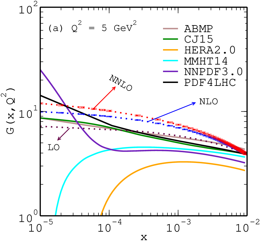
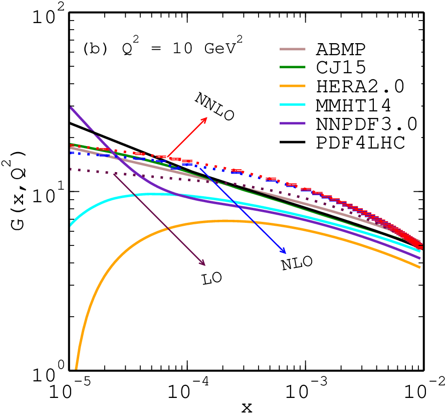
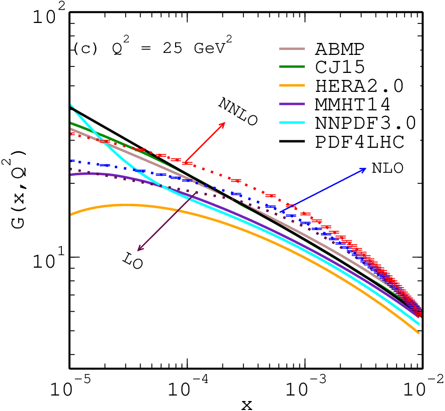
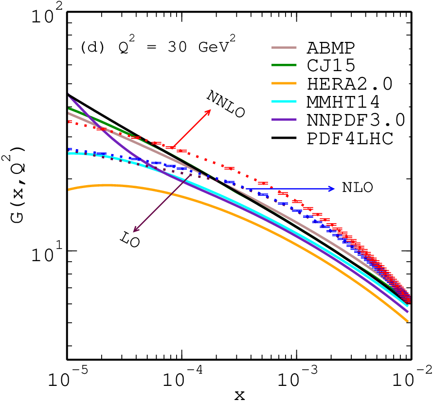
In Fig. 3(a-d), we plot our NLO as well as NNLO solutions for in the kinematics of at and respectively. It can be observed that our NNLO result lies slightly above the NLO result. This is due to the additional higher order gluon-gluon splitting terms present in the splitting function . The value of the Regge intercept is crucial in this phenomenological study. The strong coupling constant also enters into the picture through the relation [49] which can control the growth of . We have shown comparison of our results with those obtained by global DGLAP fits by various collaborations like CT14 [36], NNPDF3.0 [2], HERAPDF2.0 [1], PDF4LHC [37], ABMP16 [38] and MMHT14 [39]. We have used APFEL tool [51] to generate the gluon distribution functions of these collaborations in the kinematics of for and . We have used the LHAPDF6 [52] PDF grids to generate these data. For the best fit of results shown in Fig. 3(a-d), all the parameters that we have considered are listed in the Table II. From this figure, we have seen that while, our results are compatible and close to various groups parametrizations, our results differ significantly from the HERAPDFs. This is beacuse we have taken the input value from the PDF4LHC at , and the PDF4LHC itself seems to differ from HERAPDF as can be seen in the figure.
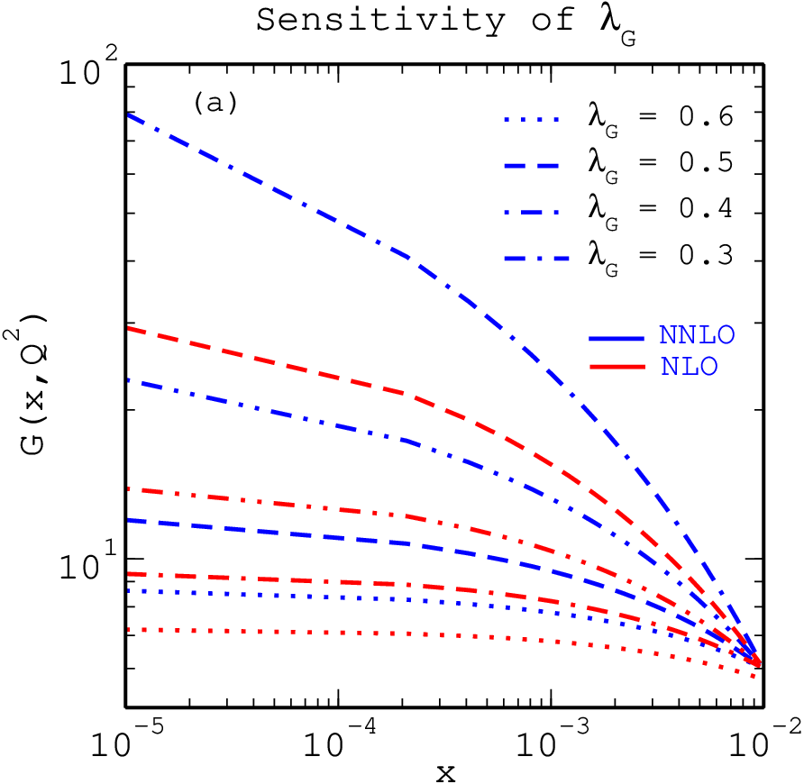
In Fig. 4(a-b), we check the sensitivity of R and on our results. In Fig. 4(a), we plot the NLO and NNLO gluon distribution functions in the same kinematic range that we are considering, for four different values of viz., 0.3, 0.4, 0.5 and 0.6 respectively. For reference we take and R = 2 respectively. We observe a sharp rise of towards small-x as we increase the value of . We notice that due to the NNLO corrections, rises faster than that of the gluon distribution function when only the NLO terms were incorporated. In Fig. 4(b) we plot the ratio () between at to at . It can be observed that the value of decrease as x decreases for a fixed-. This can be attributed to the fact that the taming of is more when the gluons are concentrated at the hotspots(R = 2 ) than when they are spread throughout the size of the proton (R = 5 ). As we increase the ratio shifts upwards as x decreases, this means the taming will be less when increases on decreasing x. This is again confirmation of the fact that the size of gluons grows as . Also, we observe that the taming is more in NNLO solution than that of the NLO solution as x decreases for a fixed-. This is due to the additional NNLO term present in the gluon-gluon splitting function . The sensitivities of the parameters and on can also be visualized in a three-dimensional picture as shown in Fig. (5).


VI Summary
In summary, in this work, we have presented a phenomenological study of the nonlinear effects of gluon distribution function, in the kinematic range of and at NLO and NNLO by solving the nonlinear GLR-MQ equation. We have employed the Regge like behavior of gluons in our calculations. We believe that our solutions are valid in the vicinity of saturation scale where it is reasonable to account for the recombination effect to show up because of very high gluon density inside the hadrons and thus our assumptions look natural too. The gluon distribution function in our solutions increases as x decreases which is in good agreement with the perturbative QCD fits at small-x. Through our results, we have verified the Regge like behavior of gluons at moderate- and small-x. It can be observed that our results show almost similar behavior from the results obtained by various global parameterization groups.
The advantage of our semi-analytical solution over the exact numerical solutions is that the functional form of the solution makes it easier to perform a phenomenological study of it with respect to various parameters in the solution. For instance, in our phenomenology , R, and are parameters, in the solutions we can easily control these parameters and we can effectively study the effect of these parameters on our results. In simple words, we can effectively manipulate or control our results by looking upon which parameters to be fixed up, by qualitatively analyzing the form of the solution.
We have also observed that our solutions are very sensitive to the Regge intercept () and the correlation radius of two interacting gluons (). It can also be observed that compared to our NLO solution, the NNLO solution is more sensitive to and R. In our phenomenological study we also showed that the taming of gluon distribution function becomes more towards small-x at low- than that of the gluon distribution function towards small-x at a larger-.
So far we have discussed how the saturation phenomenon may show up inside the hadrons at very high dense gluon regime at high energy due to nonlinear effects like the gluon recombination. Although there has been evidence of saturation from the pioneering finding of geometrical scaling in the description of experimental data at HERA [24] and in the production of comprehensive jets in the LHC data [25], but conclusive proof of saturation is yet to be seen.
The Large Hadron electron Collider (LHeC)[53] is a proposed facility which will exploit the new world of energy and intensity offered by the LHC for electron-proton scattering, through the addition of a new electron accelerator. At LHeC it is expected to reach a wider kinematic range of and which could not be explored previously. Hopefully, LHeC will give a direct evidence of saturation. Apart from probing the saturation regime it is worth mentioning that with hundred times the luminosity that was achieved at HERA, some of the salient features of the LHeC would be the determination of all light and heavy quark parton distributions for the first time, the high precision extraction of the gluon density, the determination of the strong coupling constant to per-mil accuracy and the precision study of the running of the electroweak mixing angle. LHeC thus will provide a new window on QCD and small-x physics and in this domain of small-x physics, we believe that the GLR-MQ equation will be a better candidate than the linear DGLAP equation to explain the nonlinear effects like the shadowing of gluons. Thus, we can conclude that in kinematics, where the density of gluons is very high, the GLR-MQ equation can provide a better understanding of the physical picture than the linear DGLAP equation.
Acknowledgements.
M. Lalung is grateful to CSIR, New Delhi, India for CSIR Junior Research Fellowship and P. Phukan acknowledges DST, Govt. of India for Inspire fellowship.References
- [1] H. Abramowicz et al., The European Physical Journal C 75, 580 (2015).
- [2] R. D. Ball et al., Journal of High Energy Physics 2015, 40 (2015).
- [3] H. L. Lai, J. Huston, S. Kuhlmann, F. Olness, J. Owens, D. Soper, W. K. Tung, and H. Weerts, Phys. Rev. D 55, 1280 (1997).
- [4] M. Hirai and S. Kumano, Nuclear Physics B 813, 106 (2009).
- [5] A. Manashov, M. Kirch, and A. Schäfer, Phys. Rev. Lett. 95, 012002 (2005).
- [6] R. D. Ball, M. Bonvini, S. Forte, S. Marzani, and G. Ridolfi, Nuclear Physics B 874, 746 (2013).
- [7] G. Altarelli and G. Parisi, Nuclear Physics B 126, 298 (1977).
- [8] E. Kuraev, L. Lipatov, and V. Fadin, Sov. Phys. JETP 44 (1976).
- [9] E. Kuraev, L. Lipatov, and V. Fadin, Sov. Phys. JETP 45 (1977).
- [10] Y. Balitsky and L. Lipatov, Sov. J. Nucl. Phys. 28 (1978).
- [11] C. Adloff et al., Physics Letters B 520, 183 (2001).
- [12] C. Adloff et al., The European Physical Journal C - Particles and Fields 13, 609 (2000).
- [13] C. Adloff et al., The European Physical Journal C - Particles and Fields 21, 33 (2001).
- [14] S. Chekanov et al., The European Physical Journal C - Particles and Fields 21, 443 (2001).
- [15] A. Cafarella, C. Corianò, and M. Guzzi, Nuclear Physics B 748, 253 (2006).
- [16] R. Baishya, U. Jamil, and J. K. Sarma, Phys. Rev. D 79, 034030 (2009).
- [17] N. H. Shah and J. K. Sarma, Phys. Rev. D 77, 074023 (2008).
- [18] S. Zarrin and G. Boroun, Nuclear Physics B 922, 126 (2017).
- [19] H. Khanpour, A. Mirjalili, and S. A. Tehrani, Phys. Rev. C 95, 035201 (2017).
- [20] G. Boroun and S. Zarrin, The European Physical Journal Plus 128, 119 (2013).
- [21] G. Boroun, The European Physical Journal A 42, 251 (2009).
- [22] M. Froissart, Phys. Rev. 123, 1053 (1961).
- [23] A. Martin, Phys. Rev. 129, 1432 (1963).
- [24] A. M. Staśto, K. Golec-Biernat, and J. Kwieciński, Phys. Rev. Lett. 86, 596 (2001).
- [25] M. Praszalowicz, Phys. Rev. Lett. 106, 142002 (2011).
- [26] S. Benić, K. Fukushima, O. Garcia-Montero, and R. Venugopalan, Journal of High Energy Physics 2017, 115 (2017).
- [27] W. Zhu and J. Lan, Nuclear Physics B 916, 647 (2017).
- [28] A. Mueller, Nuclear Physics B 558, 285 (1999).
- [29] S. Chekanov et al. (ZEUS Collaboration), Phys. Rev. D 67, 012007 (2003).
- [30] L. Gribov, E. Levin, and M. Ryskin, Physics Reports 100, 1 (1983).
- [31] A. Mueller and J. Qiu, Nuclear Physics B 268, 427 (1986).
- [32] A. Mueller, Nuclear Physics B 415, 373 (1994).
- [33] A. Mueller, Nuclear Physics B 437, 107 (1995).
- [34] M. Lalung, P. Phukan, and J. K. Sarma, International Journal of Theoretical Physics 56, 3625 (2017).
- [35] P. Phukan, M. Lalung, and J. K. Sarma, Nuclear Physics A 968, 275 (2017).
- [36] S. Dulat, T.-J. Hou, J. Gao, M. Guzzi, J. Huston, P. Nadolsky, J. Pumplin, C. Schmidt, D. Stump, and C.-P. Yuan, Phys. Rev. D 93, 033006 (2016).
- [37] J. Rojo et al., Journal of Physics G: Nuclear and Particle Physics 42, 103103 (2015).
- [38] S. Alekhin et al., Phys. Rev. D 96, 014011 (2017).
- [39] L. A. Harland-Lang, A. D. Martin, P. Motylinski, and R. S. Thorne, The European Physical Journal C 75, 204 (2015).
- [40] E. Laenen and E. Levin, Nuclear Physics B 451, 207 (1995).
- [41] K. Prytz, The European Physical Journal C 22, 317 (2001).
- [42] M. Devee and J. K. Sarma, Nuclear Physics B 885, 571 (2014).
- [43] A. Donnachie and P. Landshoff, Physics Letters B 437, 408 (1998).
- [44] J.-R. Cudell, A. Donnachie, and P. Landshoff, Physics Letters B 448, 281 (1999).
- [45] A. Donnachie and P. V. Landshoff, Physics Letters B 550, 160 (2002).
- [46] V. S. Fadin, E. Kuraev, and L. Lipatov, Physics Letters B 60, 50 (1975).
- [47] R. D. Ball and P. V. Landshoff, Journal of Physics G: Nuclear and Particle Physics 26, 672 (2000).
- [48] K. Golec-Biernat, L. Motyka, and A. M. Staśto, Physical Review D 65, 074037 (2002).
- [49] J. Kwiecinski, Journal of Physics G: Nuclear and Particle Physics 19, 1443 (1993).
- [50] A. Vogt, S. Moch, and J. Vermaseren, Nuclear Physics B 691, 129 (2004).
- [51] S. Carrazza, A. Ferrara, D. Palazzo, and J. Rojo, Journal of Physics G: Nuclear and Particle Physics 42, 057001 (2015).
- [52] A. Buckley, J. Ferrando, S. Lloyd, K. Nordström, B. Page, M. Rüfenacht, M. Schönherr, and G. Watt, The European Physical Journal C 75, 132 (2015).
- [53] J. L. A. Fernandez et al., Journal of Physics G: Nuclear and Particle Physics 39, 075001 (2012).