An Exponential Time-Integrator Scheme
for Steady and Unsteady Inviscid Flows

We start with the following semi-discrete system of autonomous ordinary differential equations which may be obtained from a spatial discretization:

where $\mathbf{u}=\mathbf{u}(t)\in\mathbb{R}^{K}$ denotes the vector of the solution variables and $\mathbf{R}(\mathbf{u})\in\mathbb{R}^{K}$ the right-hand-side term which may be the spatially discretized residual terms of the discontinuous Galerkin method used in this work. The dimension $K$ is the degrees of freedom which can be very large for 3D problems. Without loss of generality, we consider $\mathbf{u}(t)$ in the interval of one time step, i.e., $t\in[t_{n},\,t_{n+1}]$.

We apply the term splitting method [26] to treat Eq. (1):

where the subscript $n$ indicates the value evaluated at $t=t_{n}$, $\bm{\mathsf{J}}_{n}$ denotes the Jacobian matrix $\bm{\mathsf{J}}_{n}:=\frac{\partial\mathbf{R}(\mathbf{u})}{\partial\mathbf{u}}\Big|_{t=t_{n}}$ and $\mathbf{N}(\mathbf{u}):=\mathbf{R}(\mathbf{u})-\bm{\mathsf{J}}_{n}{\mathbf{u}}$ denotes the reminder, which in general is nonlinear. Equation (2) admits the following formal solution:

where $\Delta t:=t_{n+1}-t_{n}$ and

is the integrating factor. The formal solution (3) is the starting point to derive the proposed exponential scheme in which the stiff part is computed analytically whereas the nonlinear term is approximated numerically.

By substituting the nonlinear term $\mathbf{N}(t_{n}+\tau)$ with its Taylor expansion about $t_{n}$

the solution (3) becomes

where the tensorial function $\bm{\mathsf{\Phi}}_{k}(\Delta t\bm{\mathsf{J}}_{n})$ is defined as the following:

and it satisfies the following recursion relationship:

where $\bm{\mathsf{I}}$ denotes the $K\times K$ identity matrix. Thus, an approximation of the integral in (3) by a truncated Taylor expansion of the nonlinear term $\mathbf{N}$ leads to an exponential scheme consisting of linear combinations of functions $\bm{\mathsf{\Phi}}_{k}$. Specifically, with $k=1$, the nonlinear term $\mathbf{N}$ is approximated by a constant, i.e., its left-end value $\mathbf{N}_{n}$ on the interval $[t_{n},\,t_{n+1}]$, hence,

leading to a simple exponential scheme

which is the first-order exponential-time differencing scheme, ETD1 [18], also referred as exponential Rosenbrock-Euler method [26].

With $k=2$, a first-order finite-difference approximation to the derivative of $\mathbf{N}$, i.e.,

leads to the second-order scheme ETD2 [30]:

Clearly the ETD2 scheme requires an extra term $\bm{\mathsf{\Phi}}_{2}(\Delta t\bm{\mathsf{J}}_{n})(\mathbf{N}_{n}-\mathbf{N}_{n-1})$ compared to the ETD1 scheme. It should be stressed that the calculation of $\bm{\mathsf{\Phi}}_{2}$ is computationally more demanding than that of $\bm{\mathsf{\Phi}}_{1}$ for a system with large degrees of freedom $K$. Hence, the ETD2 scheme might not be practical for large systems.

The Runge-Kutta or multi-step approximations for the nonlinear term $\mathbf{N}(\mathbf{u})$ can also be used to construct high-order schemes (cf., e.g., [18, 28, 31]). However, the objective of this work is to construct an effective and efficient second-order ETD scheme which only requires $\bm{\mathsf{\Phi}}_{1}$. To this end, we design a scheme based on the idea of the predictor-corrector methodology consisting of two stages. First, the solution is advanced with the first-order ETD scheme (10) to obtain a predicted solution $\mathbf{u}_{*}$. Next, the solution $\mathbf{u}_{n+1}$ is corrected by replacing the nonlinear term ${\mathbf{N}}_{n}:=\mathbf{N}(\mathbf{u}_{n})$ by the algebraic average of itself and its predicted solution $\mathbf{N}_{*}:=\mathbf{N}(\mathbf{u}_{*})$, which is a standard second-order Gaussian quadrature or midpoint approximation. This simple procedure enhances the accuracy of the scheme from first order to second order. The two-stage scheme can be summarized as below:

The above two-stage scheme is designated as the predictor-corrector exponential (PCEXP) scheme. The first stage of PCEXP is designated as EXP1, which is only used for steady problems. Note that the PCEXP scheme is in fact a one-step scheme, i.e., only the solution $\mathbf{u}$ at the current time $t=t_{n}$ is required.

The exponential time-integrator schemes require evaluations of matrix-vector products, and in particular, the product of the exponential functions of the Jacobian and a vector, e.g., $\bm{\mathsf{\Phi}}_{1}(\Delta t\bm{\mathsf{J}}_{n})\mathbf{N}$ in (12b). If the inverse of the Jacobian $\bm{\mathsf{J}}$ exists, then it is possible to use $\bm{\mathsf{J}}^{-1}$ to compute $\bm{\mathsf{\Phi}}_{1}(\Delta t\bm{\mathsf{J}})$ defined by (8b). However, $\bm{\mathsf{J}}$ may be singular, e.g., in the presence of periodic boundary conditions, thus $\bm{\mathsf{J}}^{-1}$ may have to be computed with an operator restriction treatment for generalized matrix inversion, such as the singular value decomposition (SVD). In addition, for a problem with a very large number of degrees of freedom, direct inversion of $\bm{\mathsf{J}}$ can be prohibitively expensive to compute. These impediments could be the reason why the exponential schemes have yet to gain much traction.

The matrix-vector products in (12b) can be approximated efficiently using the Krylov method [35, 36], which can also treat a singular $\bm{\mathsf{J}}$. The basic idea of the Krylov method is to approximate the product of $\exp(\Delta t\bm{\mathsf{J}})$ and a vector, such as $\mathbf{N}$ in (12b), by projecting it onto a small Krylov subspace, resulting in a much smaller matrix thus cheaper in computational effort. The algorithm will be discussed in detail next.

With the Taylor expansion of $\exp(\Delta t\bm{\mathsf{J}})$, the product $\bm{\mathsf{\Phi}}_{1}\mathbf{N}$ can be written as:

It can be approximated by the following function projection onto the Krylov subspace of dimension $m$:

The orthogonal basis matrix $\bm{\mathsf{V}}_{m}:=(\mathbf{v}_{1},\,\mathbf{v}_{2},\,\cdots,\,\mathbf{v}_{m})\in\mathbb{R}^{K\times m}$ satisfies the so-called Arnoldi decomposition [36]:

where $\bm{\mathsf{V}}_{m+1}:=(\mathbf{v}_{1},\,\mathbf{v}_{2},\,\cdots,\,\mathbf{v}_{m},\,\mathbf{v}_{m+1})=(\bm{\mathsf{V}}_{m},\,\mathbf{v}_{m+1})\in\mathbb{R}^{K\times(m+1)}$ and $\widetilde{\bm{\mathsf{H}}}_{m}$ is the following $(m+1)\times m$ upper- Hessenberg matrix:

The matrix $\widetilde{\bm{\mathsf{H}}}_{m}$ can be written as the following:

where $\bm{\mathsf{H}}_{m}$ is the matrix composed of the first $m$ rows of $\widetilde{\bm{\mathsf{H}}}_{m}$ and $\mathbf{e}_{m}:=(0,\,\cdots,\,0,\,1)^{\bm{\mathsf{T}}}\in\mathbb{R}^{m}$ is the $m$-th canonical basis vector in $\mathbb{R}^{m}$, then Eq. (15) becomes

Because $\bm{\mathsf{V}}_{m}^{\bm{\mathsf{T}}}\bm{\mathsf{V}}_{m}=\bm{\mathsf{I}}$, the upper-Hessenberg matrix $\widetilde{\bm{\mathsf{H}}}_{m}$ is given by:

Therefore $\bm{\mathsf{H}}_{m}$ is the projection of the linear transformation of $\bm{\mathsf{J}}$ onto the subspace $\mathbb{K}_{m}$ with the basis $\mathbb{V}_{m}$. Because $\bm{\mathsf{V}}_{m}\bm{\mathsf{V}}_{m}^{\bm{\mathsf{T}}}\neq\bm{\mathsf{I}}$, (19) leads to the following approximation:

and $\exp(\bm{\mathsf{J}})$ can be approximated by $\exp(\bm{\mathsf{V}}_{m}\bm{\mathsf{H}}_{m}\bm{\mathsf{V}}^{\bm{\mathsf{T}}}_{m})$ as the following:

The first column vector of $\bm{\mathsf{V}}_{m}$ is $\mathbf{v}_{1}=\mathbf{N}/\|\mathbf{N}\|_{2}$ and $\bm{\mathsf{V}}^{\bm{\mathsf{T}}}_{m}\mathbf{N}=\|\mathbf{N}\|_{2}\,\mathbf{e}_{1}$, thus (21) becomes:

Consequently $\bm{\mathsf{\Phi}}_{1}$ can be approximated by:

In general, the dimension of the Krylov subspace, $m$, is chosen to be much smaller than the dimension of $\bm{\mathsf{J}}$, $K$, thus $\bm{\mathsf{H}}_{m}\in\mathbb{R}^{m\times m}$ can be inverted easily, so $\bm{\mathsf{\Phi}}_{1}$ can be easily computed as the following:

where the term $\exp(\Delta t\bm{\mathsf{H}}_{m})$ can be computed efficiently by the Chebyshev rational approximation (cf., e.g., [36, 37]) due to the small size of $\bm{\mathsf{H}}_{m}$.

We shall analyze the stability of the following scalar equation with a constant $J$:

Linearization of equation (25) about a fixed point $u_{0}$, such that $Ju_{0}+N(u_{0})=0$ leads to the following simple linear equation

where $u$ is now the perturbation to $u_{0}$, $\lambda=N^{\prime}(u_{0})$, and $\zeta:=J+\lambda$. Obviously, the fixed point $u_{0}$ is stable if and only if

To analyze the dependence of the stability region on the finite-term Krylov basis approximation, we apply the PCEXP scheme (12) to the model equation (26) and we obtain the following very simple solution:

Note that the solution of the linear equation produced by the PCEXP scheme is the exact solution of the same linear equation in a standard exponential form. This capability of producing the exact solution of a linear equation is an important feature of exponential schemes. The function $G$ can be approximated by its Taylor expansion up to $m$-th order:

The polynomial $G_{m}$ approximates the growth rate $G$, and the stability criterion (27) requires that $|G_{m}|\leq 1$.

We compute the dependence of the stability region determined by $|G_{m}|\leq 1$ in the parameter space $(\Delta t,\,\zeta)$ on the order of the polynomial $G_{m}$, $m$. First, for real $\zeta$, we compute the boundary of the stability region with $1\leq m\leq 80$. The $m$-dependence of the stability boundary in the parameter space $(\Delta t,\,\zeta)$ is shown in Fig. 1(a); the stability region is bounded by both $\Delta t$ and $\zeta$ axes and the $m$-dependent boundary. Clearly, the the stability region expands as $m$ increases. We also compute the $m$-dependence of the maximum stable value of $|\Delta t\zeta|$, as shown in Fig. 1(b). It can be seen that the maximum stable value of $|\Delta t\zeta|$ increases with $m$ linearly, for the linear problem considered. The result of Fig. 1(b) is also tabulated in Table 1, which also gives the $m$-dependent time-step sizes normalized by $\Delta t_{1}$ corresponding to $m=1$.

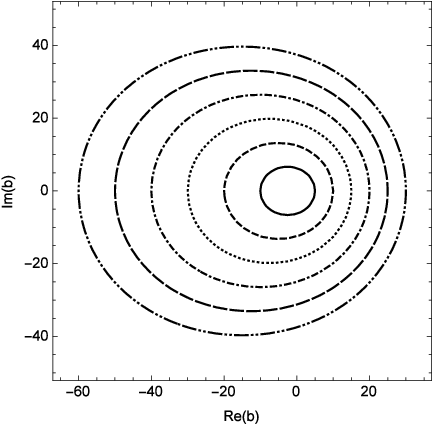
For complex $\zeta$, the boundary of the stability region is defined in the complex plane of $\Delta t\zeta$. As shown in Fig. 2, the stability region is approximately a semicircle on the left half of the complex plane $\zeta$, and the radius of the semicircle grows linearly as $m$ increases.

The preceding analysis shows the effect of the number of the terms in the Taylor expansion of the propagator, $\exp(\Delta t\zeta)$, on the stability of the exponential scheme. Next, we analyze the stability of the PCEXP scheme (12) by using the model problem (26). Applying the PCEXP scheme of (12) to (26), we have:

where $a:=\Delta t\,\lambda$ and $b:=\Delta t\,J$. The Taylor expansion of $r$ in terms of $b$ is

In the limit that $b\rightarrow{0}$, the growth factor $r$ converges to the leading term of (31)

which is identical to the second-order Runge-Kutta scheme.

The above analysis directly shows the following two important features of the PCEXP scheme in the limits of $N\rightarrow 0$ and $J\rightarrow 0$:

1. 1.

   The PCEXP scheme reduces to the exact solution of the linear equation in the limit of vanishing nonlinear term $N\rightarrow 0$, as shown by (28);

2. 2.

   The PCEXP scheme converges to the second-order Runge-Kutta scheme in the limit of vanishing linear term $J\rightarrow{0}$, as shown by (32).

We now consider the dependence of the stability region on the parameter $a:=\Delta t\,\lambda$ and $b:=\Delta t\,J$. For real $a$ and $b$, the boundary of the stability region is defined by $|r|=1$. For the PCEXP scheme, $r$ is given by (30), and $|r|\leq 1$ leads to

For the EXP1 scheme,

then the corresponding stability region is bounded by

Similarly, for the TVDRK3 scheme

so its stability region is a strip bounded by two parallel lines:

The stability regions of PCEXP, EXP1, and TVDRK3 are illustrated in Fig. 3.

The stability region of the PCEXP scheme is larger than that of the EXP1 scheme, therefore the PCEXP scheme is not only more accurate but also is better in terms of stability. Note that the stability regions of EXP1 and PCEXP schemes are infinitely large fan-shaped areas without a lower bound, while the TVDRK3 scheme in Fig. 3 (right) is a narrow strip. They imply that given a negative $J$ and a fixed $\lambda$ inside the regions, both EXP1 and PCEXP allow an infinity large $\Delta t$, while TVDRK3 does not. This stability feature distinguishes the exponential schemes from the TVDRK3 scheme.

We can also consider the stability of (30) with a complex $b=\Delta t\,J$ and a real $a=\Delta t\,\lambda$, as shown in Fig. 4. The stability region of the PCEXP scheme increases as $|\lambda|$ increases, while that of the TVDRK3 scheme only shifts a distance along the real axis on the complex $b$-plane but without changing its area. Thus, the stability region of the TVDRK3 scheme does not expand under the constraint of $b$. Clearly, the PCEXP scheme is far more superior than the TVDRK3 scheme in terms of stability, as expected.

We study the local truncation error of the PCEXP scheme by using the model scalar equation (26). The Taylor expansion of the solution (28) of the linearized equation (26), $u_{n+1}$, at $t=t_{n}$ is

where $u_{n}^{(k)}$ is the $k$-th order derivative of $u(t)$ evaluated at $t=t_{n}$, and we have used the fact that for the linearized equation of (26),

By substitution of the Taylor expansion of the exponential term $e^{\Delta t\zeta}$ in the solution (28) obtained by the PCEXP scheme (12) yields

The difference between the Taylor expansion (38) and the approximated solution (40) for $u_{n+1}$ yields the local truncation error:

Similarly, the leading-order local truncation error of the EXP1 scheme is

Obviously, the accuracy of the PCEXP scheme is one-order higher than the ETD1 scheme in the frame of classical truncation error analysis.

Consider the Euler equations in a rotating frame of reference in $d$ dimensional space:

where $\mathbf{U}\in\mathbb{R}^{d+2}$ stands for the vector of conservative variables, $\bm{\mathsf{F}}\in\mathbb{R}^{(d+2)\times d}$ the convective flux, and $\mathbf{S}\in\mathbb{R}^{d+2}$ the source term:

where $\bm{v}:=(u,\,v,\,w)^{\bm{\mathsf{T}}}$ is the absolute velocity, $\bm{\omega}:=(\omega_{x},\,\omega_{y},\,\omega_{z})^{\bm{\mathsf{T}}}$ is the angular velocity of the rotating frame of reference, $\bm{v}_{r}:=\bm{\omega}\times\bm{x}$; $\rho$, $p$, and $e$ denote the flow density, pressure, and the specific internal energy; $E=e+\frac{1}{2}||\bm{v}||^{2}$ and $H=E+p/\rho$ denote the total energy and total enthalpy, respectively; $\bm{\mathsf{I}}$ denotes the $d\times d$ unit matrix; and the pressure $p$ is given by the equation of state for a perfect gas:

where $\gamma=7/5$ is the ratio of specific heats for perfect gas.

The computational domain $\Omega$ is divided into a set of non-overlapping elements of arbitrary shape. We seek an approximation $\mathbf{U}_{h}$ in each element $E\in\Omega$ with finite dimensional space of polynomial $P^{p}$ of order $p$ in the discontinuous finite element space

The numerical solution of $\mathbf{U}_{h}$ can be approximated in the finite element space $\mathbb{V}_{h}$

In the weak formulation, the Euler equations (43) in an element $E$ becomes:

where $\hat{\bm{n}}$ is the out-normal unit vector of the surface element $\bm{\sigma}$ with respect to the element $E$, $\widetilde{\bm{\mathsf{F}}}$ is the Riemann flux [38], which will be approximated by Roe’s flux [39], and the Einstein summation convention is used. For an orthonormal basis $\{\psi_{i}\}$, the term on the left-hand side of Eq. (48) becomes diagonal, so the system is in the standard ODE form of Eq. (1), thus avoiding solving a linear system as required for a non-orthogonal basis. More importantly, the use of orthogonal basis would yield more accurate solutions, especially for high-order methods with $p\gg 2$.

In this paper, the basis function $\psi_{i}(\bm{x})$ is defined on the global Cartesian coordinate $\bm{x}:=(x,\,y,\,z)$ rather than on the cell-wise, local reference coordinates. The variable values on the Gaussian quadrature points for computing the surface fluxes can be easily accessed without the Jacobian mapping between the local reference coordinates to the global Cartesian ones [40, 41], and it also makes the discontinuous Galerkin method feasible on arbitrary polyhedral grids [42].

A simple choice of the basis function in (47) may be the monomials [43] or Taylor basis [44]. However, in the case of distorted meshes, the non-orthogonality of these basis functions may yield an ill-conditioned mass matrix, resulting in degradation of accuracy and even loss of numerical stability. In this work, to construct an orthonormal basis set $\{\psi_{i}(\bm{x})\}$, we start with the normalized monomials $\{\chi_{i}(\bm{x})\}$:

where

and the total number of basis functions $N=(p+1)(p+2)(p+3)/6$ for the $p$-th order DG approximation in 3D space. With the following definition of the inner product on an element $E$: $\left\langle f,\,g\right\rangle_{E}:=\int_{E}f\left(\bm{x}\right)g\left(\bm{x}\right)\,\mathrm{d}\bm{x},$ the coefficients $\{s_{i}\}$ and $\{c_{ij}\}$ can be computed with the modified Gram-Schmidt (MGS) orthogonalization described in the Algorithm 1.

The convergence rate and stability of the PCEXP scheme rely on the accuracy to approximate the Jacobian matrix $\bm{\mathsf{J}}$, which is directly determined by the local truncation error of (41). In the PCEXP scheme, the broadcasting of global information is achieved through the exact Jacobian matrix which accurately includes the information of both the interior and the boundary of the elements. The details of computing the exact Jacobian is discussed next.

The diagonal Jacobian can be obtained by taking the derivative of (48) with respect to the $\mathbf{u}_{j}$ of the host cell with the label “L”:

Similarly, the off-diagonal Jacobian can be obtained by taking the derivative of (48) with respect to the $\mathbf{u}_{j}$ of the neighboring cells around the host cell “L”, which is marked with the label “R”:

The Riemann flux Jacobian matrices $\partial\widetilde{\bm{\mathsf{F}}}(\mathbf{U}_{\rm L},\,\mathbf{U}_{\rm R})/\partial\mathbf{U}_{\rm L}$, $\partial\widetilde{\bm{\mathsf{F}}}(\mathbf{U}_{\rm L},\,\mathbf{U}_{\rm R})/\partial\mathbf{U}_{\rm R}$ in (50) and (51) are evaluated exactly through the automatic differentiation (AD), others can be derived easily.

The global Jacobian matrix $\bm{\mathsf{J}}$ is made of the diagonal and off-diagonal matrices above. When ${\bm{\sigma}}$ is an interior face, the flux $\widetilde{\bm{\mathsf{F}}}(\mathbf{U}_{\rm L},\,\mathbf{U}_{\rm R})$ is calculated with Roe’s Riemann solver [39]. When $\bm{\sigma}$ is a boundary face with a appropriate boundary condition, one has

where $\mathbf{U}_{\rm{ghost}}$ is a function of $\mathbf{U}_{\rm L}$ corresponding the boundary condition, and $\widetilde{\bm{\mathsf{F}}}$ is also consistently computed by the same Roe’s Riemann solver used on the interior faces. Then, the boundary flux Jacobian matrix can be expressed as

The Jacobian matrix $\bm{\nabla}\psi_{j}\,{\partial\bm{\mathsf{F}}}/{\partial\mathbf{U}}$ in the volume integration and the source-term Jacobian matrix ${\partial\mathbf{S}}/{\partial\mathbf{U}}$ are given by (62) and (64), respectively, in the Appendix. The Jacobians $\partial\widetilde{\bm{\mathsf{F}}}/\partial\mathbf{U}_{\rm L}$, $\partial\widetilde{\bm{\mathsf{F}}}/\partial\mathbf{U}_{\rm ghost}$ and $\partial\mathbf{U}_{\rm ghost}/\partial\mathbf{U}_{\rm L}$ are obtained exactly by the automatic differentiation (AD).

The vortex transportation by a uniform flow of velocity $(U_{\infty},\,0)$ [16] is computed to test the temporal accuracy of PCEXP. The initial conditions of the flow are

References

- [1] W. Reed, T. Hill, Anisotropic refinement algorithms for finite elements, Tech. Rep. LA-UR-73-479, Los Alamos National Laboratories (1973).
- [2] P. Lesaint, P. Raviart, On a Finite Element Method for Solving the Neutron Transport Equation, Mathematical Aspects of Finite Elements in Partial Differential Equations, Academic Press, 1974.
- [3] B. Cockburn, C.-W. Shu, TVB Runge-Kutta local projection discontinuous Galerkin finite element method for conservation laws, II. General framework, Math. Comput. 52 (186) (1989) 411–435.
- [4] K. Bey, J. Oden, A Runge-Kutta discontinuous finite element method for high speed flows, Tech. Rep. AIAA-1991-1575, AIAA (1991).
- [5] F. Bassi, S. Rebay, High-order accurate discontinuous finite element solution of the 2D Euler equations, J. Comput. Phys. 138 (2) (1997) 251–285.
- [6] B. Cockburn, C.-W. Shu, The Runge-Kutta discontinuous Galerkin method for conservation laws V: Multidimensional systems, J. Comput. Phys. 141 (2) (1998) 199–224.
- [7] B. Cockburn, C.-W. Shu, The local discontinuous Galerkin method for time-dependent convection-diffusion systems, SIAM J. Numer. Anal. 35 (6) (1998) 2440–2463.
- [8] D. N. Arnold, F. Brezzi, B. Cockburn, D. Marini, Discontinuous Galerkin methods for elliptic problems, in: Discontinuous Galerkin Methods, Springer, New York, 2000, pp. 89–101.
- [9] B. Cockburn, G. Karniadakis, C.-W. Shu (Eds.), Discontinuous Galerkin methods. Theory, Computation and Applications, Vol. 11 of Lecture Notes in Computational Science and Engineering, Springer, Berlin, 2000.
- [10] J. Hesthaven, T. Warburton, Nodal Discontinuous Galerkin Methods: Algorithms, Analysis, and Applications, Springer, New York, 2007.
- [11] S. Ii, F. Xiao, High order multi-moment constrained finite volume method. Part I: Basic formulation, J. Comput. Phys. 228 (10) (2009) 3669–3707.
- [12] H. Huynh, A flux reconstruction approach to high-order schemes including discontinuous Galerkin methods, Tech. Rep. AIAA-2007-4079, AIAA (2012).
- [13] Z.J. Wang, H. Gao, A unifying lifting collocation penalty formulation including the discontinuous Galerkin, spectral volume/difference methods for conservation laws on mixed grids, J. Comput. Phys. 228 (21) (2009) 8161–86.
- [14] H. Huynh, Z.J. Wang, P. E. Vincent, High-order methods for computational fluid dynamics: A brief review of compact differential formulations on unstructured grids, Comput. Fluids 98 (2014) 209–220.
- [15] C.-W. Shu, An Overview on High Order Numerical Methods for Convection Dominated PDEs, Hyperbolic Problems: Theory, Numerics, Applications, Springer, 2002.
- [16] Z.J. Wang, K. Fidkowski, R. Abgrall, F. Bassi, D. Caraeni, A. Cary, H. Deconinck, R. Hartmann, K. Hillewaert, H. Huynh, N. Kroll, G. May, P.-O. Persson, B. van Leer, M. Visbal, High-order CFD methods: Current status and perspective, Int. J. Numer. Methods Fluids 72 (8) (2013) 811–845.
- [17] Z.J. Wang, H. Huynh, A review of flux reconstruction or correction procedure via reconstruction method for the Navier-Stokes equations, Mech. Eng. Rev. 3 (1) (2016) 15–00475.
- [18] S. Cox, P. Matthews, Exponential time differencing for stiff systems, J. Comput. Phys. 176 (2) (2002) 430–455.
- [19] M. Hochbruck, C. Lubich, On Krylov subspace approximations to the matrix exponential operator, SIAM J. Numer. Anal. 34 (5) (1997) 1911–1925.
- [20] M. Hochbruck, C. Lubich, H. Selhofer, Exponential integrators for large systems of differential equations, SIAM J. Sci. Comput. 19 (5) (1998) 1552–1574.
- [21] A. Ostermann, M. Thalhammer, W. Wright, A class of explicit exponential general linear methods, BIT Numer. Math 46 (2) (2006) 409–431.
- [22] M. Tokman, Efficient integration of large stiff systems of ODEs with exponential propagation iterative (EPI) methods, J. Comput. Phys. 213 (2) (2006) 748–776.
- [23] Q. Nie, Y.-T. Zhang, R. Zhao, Efficient semi-implicit schemes for stiff systems, J. Comput. Phys. 214 (2) (2006) 521–537.
- [24] Q. Nie, F. Wan, Y.-T. Zhang, X.-F. Liu, Compact integration factor methods in high spatial dimensions, J. Comput. Phys. 227 (10) (2008) 5238–5255.
- [25] S. Chen, Y.-T. Zhang, Krylov implicit integration factor methods for spatial discretization on high dimensional unstructured meshes: Application to discontinuous Galerkin methods, J. Comput. Phys. 230 (11) (2011) 4336–4352.
- [26] M. Caliari, A. Ostermann, Implementation of exponential Rosenbrock-type integrators, Appl. Numer. Math. 59 (3) (2009) 568–582.
- [27] M. Hochbruck, A. Ostermann, J. Schwitzer, Exponential Rosenbrock-type methods, SIAM J. Numer. Anal. 47 (1) (2009) 786–803.
- [28] M. Tokman, A new class of exponential propagation iterative methods of Runge-Kutta type (EPIRK), J. Comput. Phys. 230 (24) (2011) 8762–8778.
- [29] J. Loffeld, M. Tokman, Comparative performance of exponential, implicit, and explicit integrators for stiff systems of ODEs, J. Comput. Appl. Math. 241 (2013) 45–67.
- [30] L. Ju, L. Zhu, J. Zhang, Q. Du, Fast explicit integration factor methods for semilinear parabolic equations, J. Sci. Comput. 62 (2) (2015) 431–455.
- [31] L. Zhu, L. Ju, W. Zhao, Fast high-order compact exponential time differencing Runge-Kutta methods for second-order semilinear parabolic equations, J. Sci. Comput. 67 (3) (2016) 1043–1065.
- [32] W. Edwards, L. Tuckerman, R. Friesner, D. Sorensen, Krylov method for the incompressible Navier-Stokes equations, J. Comput. Phys. 110 (1) (1994) 82–102.
- [33] J. Schulze, P. Schmid, J. Sesterhenn, Exponential time integration using Krylov subspaces, Int. J. Numer. Methods Fluids 60 (2009) 591–609.
- [34] C. Clancy, J. Pudykiewicz, On the use of exponential time integration methods in atmospheric models, Tellus A 65 (2013) 20898.
- [35] M. Tokman, J. Loffeld, Efficient design of exponential-Krylov integrators for large scale computing, Procedia Comput. Sci. 1 (1) (2010) 229–237.
- [36] Y. Saad, Analysis of some Krylov subspace approximations to the matrix exponential operator, SIAM J. Numer. Anal. 29 (1) (1992) 209–228.
- [37] C. Moler, C. van Loan, Nineteen dubious ways to compute the exponential of a matrix, twenty-five years later, SIAM J. Numer. Anal. 45 (1) (2003) 3–49.
- [38] E. Toro, Riemann Solvers and Numerical Methods for Fluid Dynamics, Springer, 1999.
- [39] P. Roe, Approximate Riemann solvers, parameter vectors, and difference schemes, J. Comput. Phys. 43 (2) (1981) 357–372.
- [40] S. Deng, W. Cai, Analysis and application of an orthogonal nodal basis on triangles for discontinuous spectral element methods, Appl. Numer. Anal. Comput. Math. 2 (3) (2006) 326–345.
- [41] M. Bergot, M. Durufl, Higher order discontinuous Galerkin method for pyramidal elements using orthogonal bases, Numer. Meth. Part. Diff. E. 29 (1) (2013) 144–169.
- [42] L. Botti, Influence of reference-to-physical frame mappings on approximation properties of discontinuous piecewise polynomial spaces, J. Sci. Comput. 52 (3) (2012) 675–703.
- [43] A. Wolkov, C. Hirsch, N. Petrovskaya, Application of a higher order discontinuous Galerkin method in computational aerodynamics, Math. Model. Nat. Phenom. 6 (3) (2011) 237–263.
- [44] H. Luo, S. Li, Y. Xia, R. Nourgaliev, C. Cai, A Hermit WENO reconstruction-based discontinuous Galerkin method for the Euler equations on tetrahedral grids, Tech. Rep. AIAA-2012-0461, AIAA (2012).
- [45] S. Eckert, H. Baaser, D. Gross, O. Scherf, A BDF2 integration method with step size control for elasto-plasticity, Comput. Mech. 34 (5) (2004) 377–386.