A network partition method for solving large-scale complex nonlinear processes

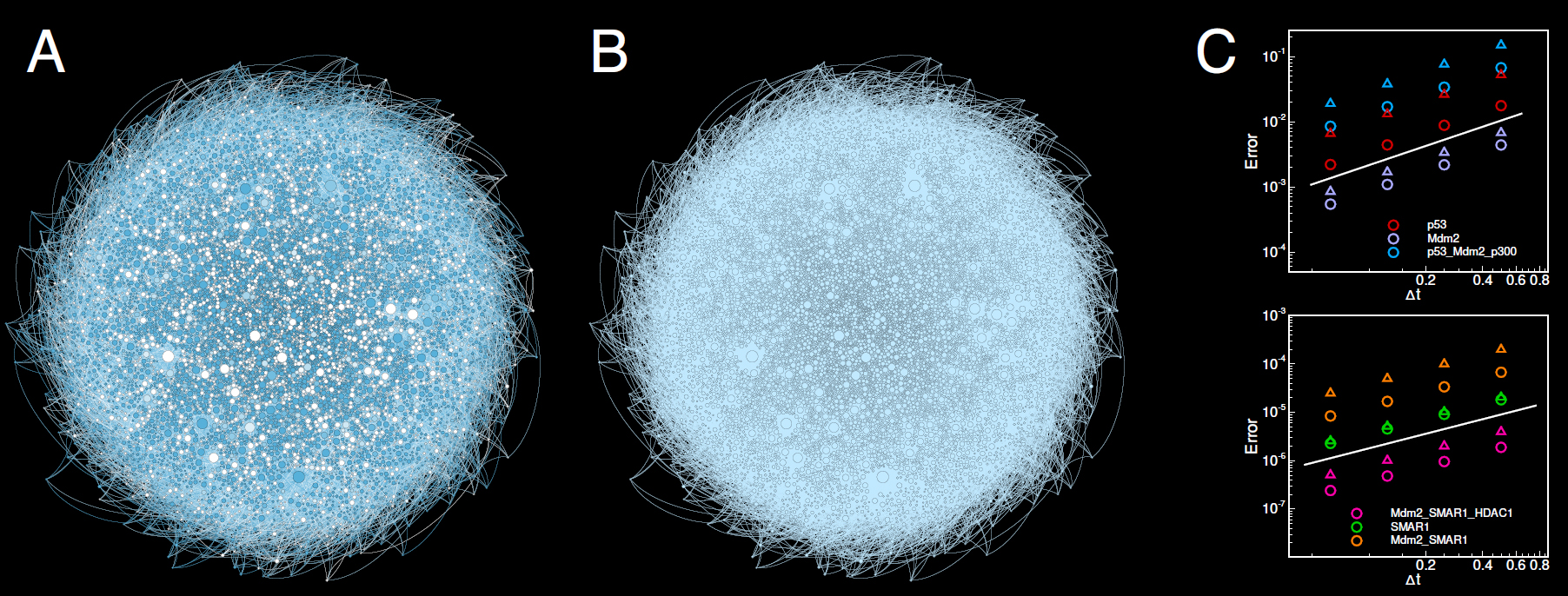
As shown in Fig.1A, a chemical reaction system with $43$ channels exhibits a network structure. In this network, each node (reaction) has multiple interactions with others by affecting the a number of reacting species. We can find a mapping $f:\Gamma\rightarrow G$ that convert the network to a graph $G=(V,E)$, where $V$ and $E$ are the set of nodes (elements) and the set of edges (pairs), respectively. For instance, one can use the definition in Fig.1B where multiple interactions between the same pair of reactions, $(x,y)$, collapse to one edge $e(x,y)$, i.e., the element $a(x,y)$ of the adjacency matrix $\mathbf{A}(G)$ is $1$ or $0$, depending on whether the reactions $x$ ad $y$ evolve common species. The degree of each node $x$, $d(x)=\sum_{y\in V}a(x,y)$, is highly heterogeneous and the distribution of edges shows sparsity, i.e., the number of edges $n(E)$ is considerably smaller than of the complete graph.

Besides, the node in $G$ can be a group of coupled elementary processes which is solvable in the sense that it has analytical solutions or is easy to be numerically solved. For example, multiple reactions in Fig.1 interacted by common product species have analytical solutions and thus can be considered as a single node in $G$, leading to a mapping different $f^{*}$. Or one define a group of reactions as a node if it is efficient to be solved by locally applying implicit time-integration methods. Then the network partition is performed to ensure there is no interaction between those small structures if they are grouped into the same subset.

Large-scale systems are too difficult to solve directly, either due to high computational cost or numerical instabilities. Instead, we apply the operator splitting method which separates the original system into a number of small-scale subsystems, with each one being easy to be numerically solved, and thus offering convenience for solving large-scale nonlinear systems. For instance, the reaction system in Fig.1 can be solved by e.g. Lie splitting method, i.e., the $N$ elementary reactions are solved individually. In this way the results are positive and conservative without time-step constraints and omits costly matrix operations [29].

When $N$ is large, the large number of splitting generates significant splitting errors which prevent the use of large time-steps. Another issue is that the operator splitting method requires a sequential updating of all $N$ subproblems. This causality leads to difficulty for parallization which is usually required for solving large-scale problems. To reduce the number of splitting and alleviate the causality of operator splitting methods, we propose a numerical framework that utilizes the sparsity of the network structure. Usually in most of large-scale systems the directly interacting elements are sparse and the elements that are not direct interacted can be solved simultaneously without numerical difficulty. This inspires us to split the original system into $K$ ($K<N$) subsystems where their elements have no direct interaction and solves the dynamics of all elements inside a certain subsystem simultaneously. This leads to a network partition problem: given a graph $G(V,E)$ after mapping from a physical system, say chemical reaction, one cluster its nodes by a partition $S=\bigcup_{k=1}^{K}S_{k}$ that satisfies

where $k$ indexes the subsets and $\mathbf{A}_{k}$ is the adjacency matrix of the $k$-th subset. This partition can be achieved by a graph coloring algorithm. When the network is mapped to a planar graph, one have $K\leqslant 4$.

After partitioning the network, the elementary processes clustered into the same subset, say $S_{k}$, generate a subproblem which can be solved in parallel, as the causality updating constraint is avoided in $S_{k}$. Consider $N_{k}$ elementary irrelevant reactions belong to the subset $S_{k}$. The $N_{k}$ processes are solved simultaneously and the updated involved species are chosen to be input of $S_{k+1}$. The entire reacting system is numerically solved by Lie splitting scheme, $\mathbf{X}^{n+1}=\mathbf{E}_{1}(\Delta t)\circ\mathbf{E}_{2}(\Delta t)\circ\mathbf{E}_{3}(\Delta t)$, if $K=3$, where $\mathbf{X}\in\mathbb{R}^{M}$ is the concentration vector and $\mathbf{E}_{k}$ is the time-integration of the subset $S_{k}$. Note that the network partition is a semi-constructive procedure and $\mathbf{E}$ can be prescribed, say the backward Euler scheme. In this paper, we use analytical solution according the type of every elementary reaction.

The splitting error arising from decoupling treatment of the original couple system can be further reduced by some existing strategies [35]. And the order of accuracy, limited to 1st order due to Lie splitting, can be increased by higher order operator splitting schemes [36, 8, 37]. Consider the widely used Strang splitting scheme [36], we can arrange the decoupled subproblems symmetrically and solve them by $\mathbf{X}^{n+1}=\mathbf{E}_{1}(\Delta t/2)\circ\mathbf{E}_{2}(\Delta t/2)\circ\mathbf{E}_{3}(\Delta t)\circ\mathbf{E}_{2}(\Delta t/2)\circ\mathbf{E}_{1}(\Delta t/2)$. The adaptive time-stepping techniques can be applied to improve the accuracy based on local errors estimation. Here we use a similar way with ref.[23] to control the local errors. We reduce the time-step if the relative error between two solutions of different level are larger than a tolerance $\varepsilon\Delta t^{k}$, where $k$ is the order of splitting method and $\varepsilon$ is a small constant. Consider the base time-step is $\Delta t$ and we perform $n^{0}_{s}$ full numerical evaluations at the coarsest level. If the refinement level is $\ell$, the time-step can be reduced to $\Delta t/(2^{\ell}n^{0}_{s})$.

And there exists a large number of partition strategies for large-scale system. Indeed, the optimal partition is the one that minimizes the splitting error, say $\frac{\Delta t^{2}}{2}[\mathbf{M}_{1},\mathbf{M}_{2}]\mathbf{X^{0}}$ for $K=2$, where $[\cdot]$ is the commutator and $\mathbf{M}$ is the operator for each subproblem. However this strategy requires applying optimization on-the-fly, which is costly for large $N$. Alternatively, we can find a partition that the most relevant nodes are clustered into the same subset. One can relate the network with a Markov chain and define a metric called “diffusion map” which measures the correlation of different nodes [20]. For a reacting system, a weight matrix that measures the pairwise interaction strength is defined as $w(x,y)=\sum_{z}\max(\alpha(x)|\nu(x,z)+\mu(x,z)|,\alpha(y)|\nu(y,z)+\mu(y,z)|)$, which assembles the connectivity measure in some reaction mechanism reduction methods [24], where $z$ labels all common species of reactions $x$ and $y$, $\alpha$ is the reaction rate coefficient, $\nu(x,z)$ is the stoichiometric coefficient of reactant $z$ in reaction $x$, and $\mu(x,z)$ is the stoichiometric coefficient of product $z$ in reaction $x$. Then the transition matrix of the corresponding Markov chain is determined by $p(x,y)=w(x,y)/\sum_{z\in G}w(x,z)$. And let $\lambda_{l}$, $\psi_{l}$ and $\phi_{l}$ be the eigenvalue, normalized right and left eigenvectors of $P$ with $0\leqslant l\leqslant N-1$. The diffusion map $\Psi_{t}(x)=[\lambda_{1}^{t}\psi_{1}(x),\,\,\lambda_{2}^{t}\psi_{2}(x),\,\,\cdots,\,\,\lambda_{q}^{t}\psi_{q}(x)]^{\text{T}}$ is introduced in ref.[20] so that one can determine the connectivity of different nodes by measuring their distance in diffusion coordinates, $D^{2}_{t}(x,y)=\|\Psi_{t}(x)-\Psi_{t}(y)\|^{2}$. Then nodes are clustered into subsets depending on their diffusion distance to the geometric centroids of subsets $c(S_{k})=\sum_{x\in S_{k}}\frac{\phi_{0}(x)}{\bar{\phi}_{0}(S_{k})}\Psi_{t}(x)$, where $\bar{\phi}_{0}(S_{k})=\sum_{x\in S_{k}}\phi_{0}(x)$. This leads to a new partition that minimizing the distortion $\sum_{k}\sum_{x\in S_{k}}\phi_{0}(x)\|\Psi_{t}(x)-c(S_{k})\|^{2}$. For our case, we follow the clustering algorithm in [20] to modify our initial partition, $S^{(0)}=\bigcup_{k=1}^{K}S^{(0)}_{k}$ which is generated by graph coloring algorithm. Then the partition becomes

which is solved by constrained k-means algorithm [39] with $p$ indexing the iteration step. Then the most relevant nodes are grouped into the same subset while maintaining the constraint $\mathbf{A}_{k}=\mathbf{0}$. Although this is not the optimal partition, it outperforms the initial partition generated by coloring algorithm in our test cases.

The current method has the following advantages when applied to large-scale complex systems:

1. 1.

   This method is unconditionally stable, provided the time-integration $\mathbf{E}$ for each subproblem is stable. Thus the chosen time-step can be very large, which offers efficiency for computations of large-scale systems.

2. 2.

   Negative concentration generation is avoided for systems with large stiffness.

3. 3.

   The number of splitting, $K$, is small for large-scale complex systems due to the sparsity feature, indicating a reduced splitting error.

4. 4.

   The method are well suited for parallel simulations as the elements of every subproblem have no direct correlation.

Given a well-stirred chemical system with $M$ chemical species which interact through $N$ reactions. If the stochastic effects in this system are neglected and the concentration vector $\mathbf{X}=\{\text{X}_{1},\text{X}_{2},\cdots,\text{X}_{M}\}^{T}$ is assumed to vary continuously in time, the time evolution of the system can be described by the reaction rate equation,

for $1\leq i\leq M$, where $\mu_{ji}$ and $\nu_{ji}$ are stoichiometric coefficients of reactant $i$ and product $i$ involved in the reaction $j$, respectively. $\text{C}_{j}(t)$ is the rate of reaction $j$ and usually determined by the law of mass action, $\text{C}_{j}(t)=\alpha_{j}\prod_{l}\text{X}_{l}(t)^{\mu_{jl}}$, where $\alpha_{j}$ is the reaction rate coefficient and the index $l$ labels all involved species in the reaction $j$. Usually the number of involved species and the reactions are enormous, which presents challenges when numerically solve the underlying kinematics. We will test our method through different types of chemical reactions, including the constant rate-coefficient reaction, temperature dependent reaction and stochastic reaction.

Reaction-diffusion process is the underlying mechanism of many pattern formulations in biological systems. Its behaviour on cellular networks can be used to model early stage morphogenesis [31]. Recently, reaction-diffusion (RD) processes on random networks with size up to $10^{3}$ nodes show significant difference from the class behaviour [27]. In this section we demonstrate our method can be used to efficiently solve RD processes on large-scale networks.

Consider a RD system defined on a complex network with $N^{*}$ nodes and $M$ different species. On each node, the local reactions change the concentrations of every species which are diffusively transported to connected nodes. The dynamic behaviour is described by

where $1\leq i\leq M$, $1\leq n\leq N^{*}$, $D_{i}$ is the diffusion rate of the species $i$ and $L_{nm}=A_{nm}-d_{n}\delta_{nm}$ is the network Laplacian matrix.

The Lie operator splitting method can be used for highly dissipative system in particle simulations of fluid mechanics whose diffusion term is handled by decoupling all fluxes for each particle and updating the solution in a pairwise manner [23]. Here we consider the flux $\text{F}^{i}_{nm}=\text{X}_{in}-\text{X}_{im}$ as the element and cluster it by the same way for chemical reactions, i.e., any two fluxes of each subset do not flow into or out of the same node. For the species $i$ and the subset $S_{k}$, the concentrations of node $n$ and $m$ are updated by $\text{X}_{in}=\text{X}_{in}-D_{i}\,\Delta t\,\text{F}^{i}_{nm}$ and $\text{X}_{im}=\text{X}_{im}-D_{i}\,\Delta t\,\text{F}^{i}_{nm}$, respectively. Thus positivity of $\mathbf{X}$ can be ensured by limiting the flux $\text{F}^{i}_{nm}=\max\left(-\text{F}_{im}/(D_{i}\,\Delta t),\min\left(\text{F}^{i}_{nm},\text{F}_{in}/(D_{i}\,\Delta t)\right)\right)$.

We first test pure diffusion process on a small scale-free network [3] with $N^{*}=200$ nodes and a mean degree $\bar{d}=12$. The diffusion rate $D=2.04$ and initially sate is $\text{X}=10+10\mathcal{U}(-0.01,0.01)$. As shown in Fig.6A, errors are measured when the system achieves the equilibrium state and exhibit first-order convergence. And our method shows better accuracy than the Lie splitting method. If we increase $D$, the numerical instabiles are observed if we use the 2nd-order Runge-Kutta scheme with large time-steps. This issue is addressed by our method, indicating that our method, like that in ref.[23], can handle highly dissipative system efficiently. Then the Brusselator reaction model [16],

is added for every node. The corresponding steady state is $\bar{\mathbf{X}}=\left\{1,2.9,1\right\}$ and will be destabilized under specific diffusion rate, leading to the Turing instability. A small perturbation $0.01\bar{\mathbf{X}}$ is imposed on $\bar{\mathbf{X}}$ initially and the diffusion rates are set as $D_{1}=D_{2}=7\times 10^{-3}$ and $D_{3}=0.161$. The convergence results in Fig.6B exhibit first order rate for $L_{1}$ and $L_{\infty}$ norms.

Then we study a large-scale RD system defined on a scale-free network with $10^{4}$ nodes with $\bar{d}=10$. The p53-SMAR1 regulatory reaction model is considered for the reaction term. The initial condition of $\mathbf{X}$ and the diffusion rate are listed in Table X. The $49986$ fluxes of this system are clustered into $569$ subsets and the partition of the chemical reaction is $S^{(0)}$ in Table IV. The initial condition of $\mathbf{X}$ and diffusion rates are listed in Table . When the diffusion rate is low ($0.1\%$ of the rates in Table), the distribution of p53 is highly heterogeneous (Fig.7A) and will be homogenized by large diffusion rate (Fig.7B). The convergence analysis is shown in Fig.7C which indicates our method is 1st-order accurate in this case and more accurate than Lie splitting method.

We provide the reaction mechanism for the cases used in the main text. First the p53-SMAR1 regulatory model that has $35$ elementary reactions is listed in Table 2. Its network is partitioned by $S^{(0)}$, $S^{(p)}$ and $S^{*,(0)}$, as shown in Table 4. The hydrogen-oxygen reaction with 9 species and 23 reversible reactions is detailed in Table 5 and the corresponding partition result is shown in Table 6. The LacZ/LacY reaction model contains 22 reactions and 23 species, as shown in Table 7. The SSA results at $t=300s$ are used for initial condition in Table 8. The 22 elementary reactions are partitioned into $5$ subsets in Table 9.

The thermochemical properties of the involved species can be obtained by empirical equations for fitting thermodynamic functions as

over a wide temperature range, where coefficients $a_{1}$ to $a_{7}$ and $b_{1,2}$ are tabulated in Table 11. For each species, the first row applies for a temperature range from 1000K to 6000 K and second row is used for temperature below 1000K. The temperature T of the mixture is updated by iteratively solving the thermodynamics relation

considering the internal energy $e$ is constant during the adiabatic process of $\Delta t$.

References

- [1] M. Asllani, J. D. Challenger, F. S. Pavone, L. Sacconi, and D. Fanelli. The theory of pattern formation on directed networks. Nat Commun, 5:4517, 2014.
- [2] D. Balcan, V. Colizza, B. Gonçalves, H. Hu, J. J. Ramasco, and A. Vespignani. Multiscale mobility networks and the spatial spreading of infectious diseases. Proc Natl Acad Sci USA, 106(51):21484–21489, 2009.
- [3] A.-L. Barabási and R. Albert. Emergence of scaling in random networks. science, 286(5439):509–512, 1999.
- [4] P. N. Brown, G. D. Byrne, and A. C. Hindmarsh. Vode: A variable-coefficient ODE solver. SIAM J Sci Comput, 10(5):1038–1051, 1989.
- [5] Y. Cao, D. T. Gillespie, and L. R. Petzold. Avoiding negative populations in explicit Poisson tau-leaping. J Chem Phys, 123(5):054104, 2005.
- [6] A. J. Chorin. A numerical method for solving incompressible viscous flow problems. J Comput Phys, 135(2):118–125, 1997.
- [7] V. Colizza, R. Pastor-Satorras, and A. Vespignani. Reaction–diffusion processes and metapopulation models in heterogeneous networks. Nat Phys, 3(4):276–282, 2007.
- [8] S. Descombes. Convergence of a splitting method of high order for reaction-diffusion systems. Math Comput, 70(236):1481–1501, 2001.
- [9] P. Deuflhard and U. Nowak. Efficient numerical simulation and identification of large chemical reaction systems. Ber Bunsenges Phys Chem, 90(11):940–946, 1986.
- [10] F. Diegelmann, S. Hickel, and N. A. Adams. Three-dimensional reacting shock–bubble interaction. Combust Flame, 181:300–314, 2017.
- [11] D. T. Gillespie. Exact stochastic simulation of coupled chemical reactions. J Phys Chem, 81(25):2340–2361, 1977.
- [12] D. T. Gillespie. Approximate accelerated stochastic simulation of chemically reacting systems. J Chem Phys, 115(4):1716–1733, 2001.
- [13] R. Glowinski, S. J. Osher, and W. Yin. Splitting Methods in Communication, Imaging, Science, and Engineering. Springer, 2017.
- [14] T. Goldstein and S. Osher. The split bregman method for L1-regularized problems. SIAM J Imaging Sci, 2(2):323–343, 2009.
- [15] X. Gou, W. Sun, Z. Chen, and Y. Ju. A dynamic multi-timescale method for combustion modeling with detailed and reduced chemical kinetic mechanisms. Combust Flame, 157(6):1111–1121, 2010.
- [16] S. Hata, H. Nakao, and A. S. Mikhailov. Dispersal-induced destabilization of metapopulations and oscillatory Turing patterns in ecological networks. Sci Rep, 4:3585, 2014.
- [17] D. J. Higham. Modeling and simulating chemical reactions. SIAM Rev, 50(2):347–368, 2008.
- [18] G. Karlebach and R. Shamir. Modelling and analysis of gene regulatory networks. Nat Rev Mol Cell Biol, 9(10):770–780, 2008.
- [19] A. M. Kierzek. STOCKS: STOChastic Kinetic Simulations of biochemical systems with Gillespie algorithm. Bioinformatics, 18(3):470–481, 2002.
- [20] S. Lafon and A. B. Lee. Diffusion maps and coarse-graining: A unified framework for dimensionality reduction, graph partitioning, and data set parameterization. IEEE Trans Pattern Anal Mach Intell, 28(9):1393–1403, 2006.
- [21] R. J. LeVeque and H. C. Yee. A study of numerical methods for hyperbolic conservation laws with stiff source terms. J Comput Phys, 86(1):187–210, 1990.
- [22] S. Lie and F. Engel. Theorie der Transformationsgruppen. 1888.
- [23] S. Litvinov, M. Ellero, X. Hu, and N. Adams. A splitting scheme for highly dissipative smoothed particle dynamics. J Comput Phys, 229(15):5457–5464, 2010.
- [24] T. Lu and C. K. Law. A directed relation graph method for mechanism reduction. Proc Combust Inst, 30(1):1333–1341, 2005.
- [25] T. Lu and C. K. Law. Toward accommodating realistic fuel chemistry in large-scale computations. Prog Energy Combust Sci, 35(2):192–215, 2009.
- [26] M. Z. Malik, M. J. Alam, R. Ishrat, S. M. Agarwal, and R. B. Singh. Control of apoptosis by SMAR 1. Mol Biosyst, 13(2):350–362, 2017.
- [27] H. Nakao and A. S. Mikhailov. Turing patterns in network-organized activator-inhibitor systems. Nat Phys, 6(7):544–550, 2010.
- [28] M. E. Newman. Communities, modules and large-scale structure in networks. Nat Phys, 8(1):25, 2012.
- [29] K. Nguyen, A. Caboussat, and D. Dabdub. Mass conservative, positive definite integrator for atmospheric chemical dynamics. Atmos Environ, 43(40):6287–6295, 2009.
- [30] E. S. Oran and J. P. Boris. Numerical simulation of reactive flow. Cambridge University Press, 2005.
- [31] H. G. Othmer and L. Scriven. Instability and dynamic pattern in cellular networks. J Theor Biol, 32(3):507–537, 1971.
- [32] J.-C. Rain, L. Selig, H. De Reuse, V. Battaglia, C. Reverdy, S. Simon, G. Lenzen, F. Petel, J. Wojcik, V. Schächter, et al. The protein–protein interaction map of helicobacter pylori. Nature, 409(6817):211–215, 2001.
- [33] D. A. Schwer, P. Lu, and W. H. Green. An adaptive chemistry approach to modeling complex kinetics in reacting flows. Combust Flame, 133(4):451–465, 2003.
- [34] M. Slack and A. Grillo. Investigation of hydrogen-air ignition sensitized by nitric oxide and by nitrogen dioxide. 1977.
- [35] R. L. Speth, W. H. Green, S. MacNamara, and G. Strang. Balanced splitting and rebalanced splitting. SIAM J Numer Anal, 51(6):3084–3105, 2013.
- [36] G. Strang. On the construction and comparison of difference schemes. SIAM J Numer Anal, 5(3):506–517, 1968.
- [37] M. Thalhammer. High-order exponential operator splitting methods for time-dependent Schrödinger equations. SIAM J Numer Anal, 46(4):2022–2038, 2008.
- [38] T. Tian and K. Burrage. Binomial leap methods for simulating stochastic chemical kinetics. J Chem Phys, 121(21):10356–10364, 2004.
- [39] K. Wagstaff, C. Cardie, S. Rogers, S. Schrödl, et al. Constrained k-means clustering with background knowledge. In Proceedings of the Eighteenth International Conference on Machine Learning, volume 1, pages 577–584, 2001.
Supporting Information (SI)
IV.1 The mechanism of chemical reactions and the partition results