∎
Observers in Kerr spacetimes: the ergoregion on the equatorial plane
Abstract
We perform a detailed analysis of the properties of stationary observers located on the equatorial plane of the ergosphere in a Kerr spacetime, including light-surfaces. This study highlights crucial differences between black hole and the super-spinner sources. In the case of Kerr naked singularities, the results allow us to distinguish between “weak” and “strong ” singularities, corresponding to spin values close to or distant from the limiting case of extreme black holes, respectively. We derive important limiting angular frequencies for naked singularities. We especially study very weak singularities as resulting from the spin variation of black holes. We also explore the main properties of zero angular momentum observers for different classes of black hole and naked singularity spacetimes.
1 Introduction
The physics of black holes (BHs) is probably one of the most complex and still controversial aspects of Einstein’s geometric theory of gravitation. Many processes of High Energy Astrophysics are supposed to involve singularities and their formation from a stellar progenitor collapse or from the merging of a binary BH system. The interaction of these sources with the matter environment, which can lead to accretion and jets emission, is the basis for many observed phenomena. As a consequence of this interaction, the singularity properties, determined generally by the values of their intrinsic spin, mass or electric charge parameters, might be modified, leading to considerable changes of the singularity itself. In this work, we concentrate our analysis on the ergoregion in the naked singularity (NS) and BH regimes of the axisymmetric and stationary Kerr solution. We are concerned also about the implications of any spin-mass ratio oscillation between the BH and the NS regimes from the viewpoint of stationary observers and their frequencies, assuming the invariance of the system symmetries (axial symmetry and time independence). One of the goals of this work is to explore the existence of spin transitions in very weak naked singularities [2], which are characterized by a spin parameter . If the collapse of a stellar object or the merging of several stellar or BH attractors lead to the formation of a naked singularity, then a total or partial destruction of the horizon may occur which should be accompanied by oscillations of the spin-to-mass ratio. Naked singularities can also appear in non-isolated BH configurations as the result of their interaction with the surrounding matter, i. e., in some transient process of the evolution of an interacting black hole. Indeed, the interaction can lead to modifications of characteristic BH parameters, for instance, through a spin-up or spin-down process which can also alter the spacetime symmetries. The details of such spin transitions, leading possibly to the destruction of the horizon, and their consequences are still an open problem.
In this work, keeping the Kerr spacetime symmetries unchanged, we focus on the variation of the dimensionless spin parameter in the region within the static limit on the equatorial plane of the attractor, this being the plane of symmetry of the Kerr solution. This special plane of the axisymmetric geometry has many interesting properties; for instance, constants of motion emerge due to the symmetry under reflection with respect to this plane; the geometry has some peculiarities that make it immediately comparable with the limiting static Schwarzschild solution, in particular, the location of the outer ergoregion boundary is independent of the spin value, and coincides with the location of the Schwarzschild horizon. There is also a clear astrophysical interest in the exploration of such a plane, as the large majority of accretion disks are considered to be located on the equatorial plane of their attractors.
From a methodological viewpoint, our analysis represents a comparative study of stationary and static observers in Kerr spacetimes for any range of the spin parameter. The findings in this work highlight major differences between the behavior of these observers in BH and NS geometries. These issues are clearly related to the most general and widely discussed problem of defining BHs, their event horizon and their intrinsic thermodynamic properties [3, 4, 5, 6, 7, 8]. Further, it seems compelling to clarify the role of the static limit and of the ergoregion in some of the well-analyzed astrophysical processes such as the singularity formation, through the gravitational collapse of a stellar “progenitor” or the merging of two BHs. Similarly, it is interesting to analyze the role of the frame-dragging effect in driving the accretion processes. In fact, the ergosphere plays an important role in the energetics of rotating black holes.
The dynamics inside the ergoregion is relevant in Astrophysics for possible observational effects, since in this region the Hawking radiation can be analyzed and the Penrose energy extraction process occurs [13, 9, 10, 11, 12]22 2 The Hawking process is essentially due to the vacuum fluctuation happening in the regions close to the BH horizon; it is not related to the properties of the ergoregion itself. The Hawking radiation is the (spontaneous) emission of thermal radiation which is created in the vacuum regions surrounding a BH, and leads to a decrease of the mass. Connected in many ways to the Unruh effects, it generally leads to the production of pairs of particles, one escaping to infinity while the other is trapped by the BH horizon. On the other hand, the Penrose energy extraction, or its wave-analogue of super-radiance, is related essentially to a classical (i.e. non quantum) phenomenon occurring in the ergoregion, , due to the frame-dragging of the spinning spacetime. In this way, energy can be extracted from the source, lowering its angular momentum. For a study of the Hawking radiation in Kerr and Kerr-Newman spacetimes see also [14]. For the actual state of the Penrose process, see [15]. Another interesting effect connected directly to the ergoregion is discussed in [16]. The mechanism, by which energy from compact spinning objects is extracted, is of great astrophysical interest and the effects occurring inside the ergoregion of black holes are essential for understanding the central engine mechanism of these processes [17, 18]. Accreting matter can even get out, giving rise, for example, to jets of matter or radiation [17, 19] originated inside the ergoregion. Another possibility is the extraction of energy from a rotating black hole through the Blandford-Znajek mechanism (see, for instance, [20, 21, 22, 23, 24, 25, 26, 27, 28, 29]). An interesting alternative scenario for the role of the Blandford-Znajek process in the acceleration of jets is presented in[30]. Further discussions on the Penrose and Blandford-Znajek processes may be found in [31, 32]. In general, using orbits entering the ergosphere, energy can be extracted from a Kerr black hole or a naked singularity. On the other hand, naked singularity solutions have been studied in different contexts in [33, 34, 35, 36, 37, 38, 45, 39, 40, 41, 44, 42]. Kerr naked singularities as particle accelerators are considered in [43]– see also [44, 45]. More generally, Kerr naked singularities can be relevant in connection to superspinars, as discussed in [44]. The stability of Kerr superspinars has been analyzed quite recently in [46], assenting the importance of boundary conditions in dealing with perturbations of NSs.
An interesting perspective exploring duality between elementary particles and black holes, pursuing quantum black holes as the link between microphysics and macrophysics, can be found in [47, 48, 49, 50]– see also [51]. A general discussion on the similarities between characteristic parameter values of BHs and NSs, in comparison with particle like objects, is addressed also in [53, 52, 54, 55]. Quantum evaporation of NSs was analyzed in [56], radiation in [57], and gravitational radiation in [58, 59, 60].
Creation and stability of naked singularities are still intensively debated [61, 62, 63, 64, 65, 66]. A discussion on the ergoregion stability can be found in [67, 68]. However, under quite general conditions on the progenitor, these analysis do not exclude the possibility that considering instability processes a naked singularity can be produced as the result of a gravitational collapse. These studies, based upon a numerical integration of the corresponding field equations, often consider the stability of the progenitor models and investigate the gravitational collapse of differentially rotating neutron stars in full general relativity [69]. Black hole formation is then associated with the formation of trapped surfaces. As a consequence of this, a singularity without trapped surfaces, as the result of a numerical integration, is usually considered as a proof of its naked singularity nature. However, the non existence of trapped surfaces after or during the gravitational collapse is not in general a proof of the existence of a naked singularity. As shown in [70], in fact, it is possible to choose a very particular slicing of spacetime during the formation of a spherically symmetric black hole where no trapped surfaces exist (see also [71]). Eventually, the process of gravitational collapse towards the formation of BHs (and therefore, more generally, the issues concerning the formation or not of a horizon and hence of NSs) is still, in spite of several studies, an open problem. There are transition periods of transient dynamics, possibly involving topological deformations of the spacetime, in which we know the past and future asymptotic regions of the spacetime, but it is still in fact largely unclear what happens during that process. The problem is wide and involves many factors as, especially in non-isolated systems, the role of matter and symmetries during collapse. Another major process that leads to black hole formation is the merging of two (or more) black holes, recently detected for the first time in the gravitational waves sector [72]. See also [73, 74] for the first observation of the probable formation of a BH from the coalescence of two neutron stars. An interesting and detailed analysis of Kerr and Kerr-Newman naked singularities in the broader context of braneworld Kerr-Newman (B-KN) spacetimes can be found in [75], where a new kind of instability, called mining instability, of some B-KN naked singularity spacetimes was found. In there, the exploration of the “causality violation region” is also faced. This is the region where the angular coordinate becomes timelike, leading eventually to closed timelike curves. Details on the relation between this region and the Kerr ergoregion can be found in the aforementioned reference.
In [53, 52, 55, 54, 2, 76], we focused on the study of axisymmetric gravitational fields, exploring different aspects of spacetimes with NSs and BHs. The results of this analysis show a clear difference between naked singularities and black holes from the point of view of the stability properties of circular orbits33 3 Test particle motion can be used to determine the topological properties of general relativistic spacetimes [77, 78, 79]. Moreover, we proved that in certain NS geometries different regions of stable timelike circular orbits are separated from each other by empty regions; this means that an accretion disk made of test particles will show a particular ring-like structure with specific topological properties.. This fact would have significant consequences for the extended matter surrounding the central source and, hence, in all processes associated with energy extraction. Indeed, imagine an accretion disk made of test particles which are moving along circular orbits on the equatorial plane of a Kerr spacetime. It turns out that in the case of a black hole the accretion disk is continuous whereas in the case of a naked singularity it is discontinuous. This means that we can determine the values of intrinsic physical parameters of the central attractor by analyzing the geometric and topological properties of the corresponding Keplerian accretion disk. In addition, these disconnected regions, in the case of a naked singularities, are a consequence of the repulsive gravity properties found also in many other black hole solutions and in some extensions or modifications of Einstein’s theory. The effects of repulsive gravity in the case of the Kerr geometry were considered in [80] and [81]. Analogies between the effects of repulsive gravity and the presence of a cosmological constant was shown also to occur in regular black hole spacetimes or in strong gravity objects without horizons [82, 83].
Several studies have already shown that it is necessary to distinguish between weak and strong naked singularities . It is also possible to introduce a similar classification for black holes; however, we prove here that only in the case of naked singularities there are obvious fundamental distinctions between these classes which are not present among the different black hole classes. Our focus is on strong BHs, and weak and very weak NSs. This analysis confirms the distinction between strong and weak NSs and BHs, characterized by peculiar limiting values for the spin parameters. Nevertheless, the existence and meaning of such limits is still largely unclear, and more investigation is due. However, there are indications about the existence of such limits in different geometries, where weak and strong singularities could appear. In [2, 53, 52, 54, 55], it was established that the motion of test particles on the equatorial plane of black hole spacetimes can be used to derive information about the structure of the central source of gravitation; moreover, typical effects of repulsive gravity were observed in the naked singularity ergoregion (see also [84, 85, 86, 34]). In addition, it was pointed out that there exists a dramatic difference between black holes and naked singularities with respect to the zero and negative energy states in circular orbits (stable circular geodesics with negative energy were for the first time discussed in [87]). The static limit would act indeed as a semi-permeable membrane separating the spacetime region, filled with negative energy particles, from the external one, filled with positive energy particles, gathered from infinity or expelled from the ergoregion with impoverishment of the source energy. The membrane is selective because it acts so as to filter the material in transient between the inner region and outside the static limit. This membrane wraps and selectively isolates the horizon in Kerr black holes and the singularity in superspinning solutions, partially isolating it from the outer region by letting selectively rotating infalling or outgoing matter to cross the static limit. As mentioned above, the ergoregion is involved in the BH spin-up and spin-down processes leading to a radical change of the dynamical structure of the region closest to the source and, therefore, potentially could give rise to detectable effects. It is possible that, during the evolutionary phases of the rotating object interacting with the orbiting matter, there can be some evolutionary stages of spin adjustment, for example, in the proximity of the extreme value () where the speculated spin-down of the BH can occur preventing the formation of a naked singularity with (see also [65, 88, 40, 89, 90, 91, 92, 93, 94, 63, 95]). The study of extended matter configurations in the Kerr ergoregion is faced for example in [96, 2]. In [96, 97, 99, 98, 100], a model of multi-accretion disks, so called ringed accretion disks, both corotating and counterrotating on the equatorial plane of a Kerr BH, has been proposed, and a model for such ringed accretion disks was developed. Matter can eventually be captured by the accretion disk, increasing or removing part of its energy and angular momentum, therefore prompting a shift of its spin [101, 64, 87, 102, 103, 104]. A further remarkable aspect of this region is that the outer boundary on the equatorial plane of the central singularity is invariant for every spin change, and coincides with the radius of the horizon of the static case. In the limit of zero rotation, the outer ergosurface coalesces with the event horizon. The extension of this region increases with the spin-to-mass ratio, but the outer limit is invariant. Although on the equatorial plane the ergoregion is invariant with respect to any transformation involving a change in the source spin (but not with respect to a change in the mass ), the dynamical structure of the ergoregion is not invariant with respect to a change in the spin-to-mass ratio. Nevertheless, concerning the invariance of this region with respect to spin shifts it has been argued, for example in [105], that the ergoregion cannot indeed disappear as a consequence of a change in spin, because it may be filled by negative energy matter provided by the emergence of a Penrose process44 4 We note that the wave analog of the Penrose process is the superradiant scattering. [13]. The presence of negative energy particles, a distinctive feature of the ergoregion of any spinning source in any range of the spin value, has special properties when it comes to the circular motion in weakly rotating naked singularities. The presence of this special matter in an “antigravity” sphere, possibly filled with negative energy formed according to the Penrose process, and bounded by orbits with zero angular momentum, is expected to play an important role in the source evolution. In this work, we clarify and deepen those results, formulate in detail those considerations, analyze the static limit, and perform a detailed study of this region from the point of view of stationary observers. In this regards, we mention also the interesting and recent results published in [106] and [107].
In detail, this article is organized as follows: in Sec. 2 we discuss the main properties of the Kerr solution and the features of the ergoregion in the equatorial plane of the Kerr spacetimes. Concepts and notation used throughout this work are also introduced. Stationary observers in BH and NS geometries are introduced in Sec. 3. Then, in Sec. 4, we investigate the case of zero angular momentum observers and find all the spacetime configurations in which they can exist. Finally, in Sec. 5, we discuss our results.
2 Ergoregion properties in the Kerr spacetime
The Kerr metric is an axisymmetric, stationary (nonstatic), asymptotically flat exact solution of Einstein’s equations in vacuum. In spheroidal-like Boyer–Lindquist (BL) coordinates, the line element can be written as
| (1) | |||
| (2) |
The parameter is interpreted as the mass parameter, while the rotation parameter (spin) is the specific angular momentum, and is the total angular momentum of the gravitational source. The spherically symmetric (static) Schwarzschild solution is a limiting case for .
A Kerr black hole (BH) geometry is defined by the range of the spin-mass ratio , the extreme black hole case corresponds to , whereas a super-spinner Kerr compact object or a naked singularity (NS) geometry occurs when .
The Kerr solution has several symmetry properties. The Kerr metric tensor (1) is invariant under the application of any two different transformations: where is one of the coordinates or the metric parameter while a single transformation leads to a spacetime with an opposite rotation with respect to the unchanged metric. The metric element is independent of the coordinate and the angular coordinate . The solution is stationary due to the presence of the Killing field and the geometry is axisymmetric as shown by the presence of the rotational Killing field .
An observer orbiting, with uniform angular velocity, along the curves constant and constant will not see the spacetime changing during its motion. As a consequence of this, the covariant components and of the particle four--momentum are conserved along the geodesics55 5 We adopt the geometrical units and the signature , Greek indices run in . The four-velocity satisfy . The radius has units of mass , and the angular momentum units of , the velocities and with and . For the sake of convenience, we always consider a dimensionless energy and effective potential and an angular momentum per unit of mass . and we can introduce the constants of motion
| (3) |
The constant of motion (along geodesics) is interpreted as the angular momentum of the particle as measured by an observer at infinity, and we may interpret , for timelike geodesics, as the total energy of a test particle coming from radial infinity, as measured by a static observer located at infinity.
As a consequence of the metric tensor symmetry under reflection with respect to the equatorial hyperplane , the equatorial (circular) trajectories are confined in the equatorial geodesic plane. Several remarkable surfaces characterize these geometries: For black hole and extreme black hole spacetimes the radii
| (4) |
are the event outer and inner (Killing) horizons66 6 A Killing horizon is a null surface, , whose null generators coincide with the orbits of an one-parameter group of isometries (i. e., there is a Killing field which is normal to ). Therefore, it is a lightlike hypersurface (generated by the flow of a Killing vector) on which the norm of a Killing vector goes to zero. In static BH spacetimes, the event, apparent, and Killing horizons with respect to the Killing field coincide. In the Schwarzschild spacetime, therefore, is the Killing horizon with respect to the Killing vector . The event horizons of a spinning BH are Killing horizons with respect to the Killing field , where is defined as the angular velocity of the horizon. In this article we shall extensively discuss this special vector in the case of NS geometries. We note here that the surface gravity of a BH may be defined as the rate at which the norm of the Killing vector vanishes from the outside. The surface gravity, , is a conformal invariant of the metric, but it rescales with the conformal Killing vector. Therefore, it is not the same on all generators (but obviously it is constant along one specific generator because of the symmetries). , whereas
| (5) |
are the outer and inner ergosurfaces, respectively77 7 In the Kerr solution, the Killing vector , representing time translations at infinity, becomes null at the outer boundary of the ergoregion, , which is however a timelike surface; therefore, is not a Killing horizon. More precisely, on the ergosurfaces the time translational Killing vector becomes null., with . In an extreme BH geometry, the horizons coincide, , and the relation is valid on the rotational axis (i.e., when ).
In this work, we will deal particularly with the geometric properties of the ergoregion ; in this region, we have that on the equatorial plane and also and . The outer boundary is known as the static (or also stationary) limit [108]; it is a timelike surface except on the axis of the Kerr source where it matches the outer horizon and becomes null-like. On the equatorial plane of symmetry, and the spacetime singularity is located at . In the naked singularity case, where the singularity at is not covered by a horizon, the region has a toroidal topology centered on the axis with the inner circle located on the singularity. On the equatorial plane, as the geometry “smoothly" resembles the spherical symmetric case, , and the frequency of the signals emitted by an infalling particle in motion towards , as seen by an observer at infinity, goes to zero.
In general, for and , the metric component changes its sign and vanishes for (and ). In the ergoregion, the Killing vector becomes spacelike, i.e., . As the quantity , introduced in Eq. (3), is associated to the Killing field , then the particle energy can be also negative inside . For stationary spacetimes () in , the motion with is not possible and all particles are forced to rotate with the source, i.e., . This fact implies in particular that an observer with four-velocity proportional to so that , (the dot denotes the derivative with respect to the proper time along the trajectory), cannot exist inside the ergoregion. Therefore, for any infalling matter (timelike or photonlike) approaching the horizon in the region , it holds that and , implying that the world-lines around the horizon, as long as , are subjected to an infinite twisting. On the other hand, trajectories with and (particles crossing the static limit and escaping outside in the region ) are possible.
Concerning the frequency of a signal emitted by a source in motion along the boundary of the ergoregion , it is clear that the proper time of the source particle is not null88 8 However, since , it is also known as an infinity redshift surface; see, for example, [108].. Then, for an observer at infinity, the particle will reach and penetrate the surface , in general, in a finite time . For this reason, the ergoregion boundary is not a surface of infinite redshift, except for the axis of rotation where the ergoregion coincides with the event horizon [109, 2]. This means that an observer at infinity will see a non-zero emission frequency. In the spherical symmetric case , however, as the proper time interval goes to zero as one approaches . For a timelike particle with positive energy (as measured by an observer at infinity), it is possible to cross the static limit and to escape towards infinity. In Sec. 3, we introduce stationary observers in BH and NS geometries. We find the explicit expression for the angular velocity of stationary observers, and perform a detailed analysis of its behavior in terms of the radial distance to the source and of the angular momentum of the gravity source. We find all the conditions that must be satisfied for a light-surface to exist.
3 Stationary observers and light surfaces
We start our analysis by considering stationary observers which are defined as observers whose tangent vector is a spacetime Killing vector; their four-velocity is therefore a linear combination of the two Killing vectors and , i.e., the coordinates and are constants along the worldline of a stationary observer [110]. As a consequence of this property, a stationary observer does not see the spacetime changing along its trajectory. It is convenient to introduce the (uniform) angular velocity as
| (6) |
which is a dimensionless quantity. Here, is a normalization factor
| (7) |
where . The particular case defines static observers; these observers cannot exist in the ergoregion.
The angular velocity of a timelike stationary observer () is defined within the interval
| (8) | |||
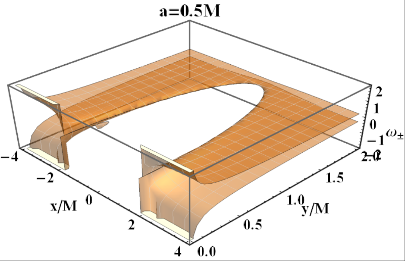
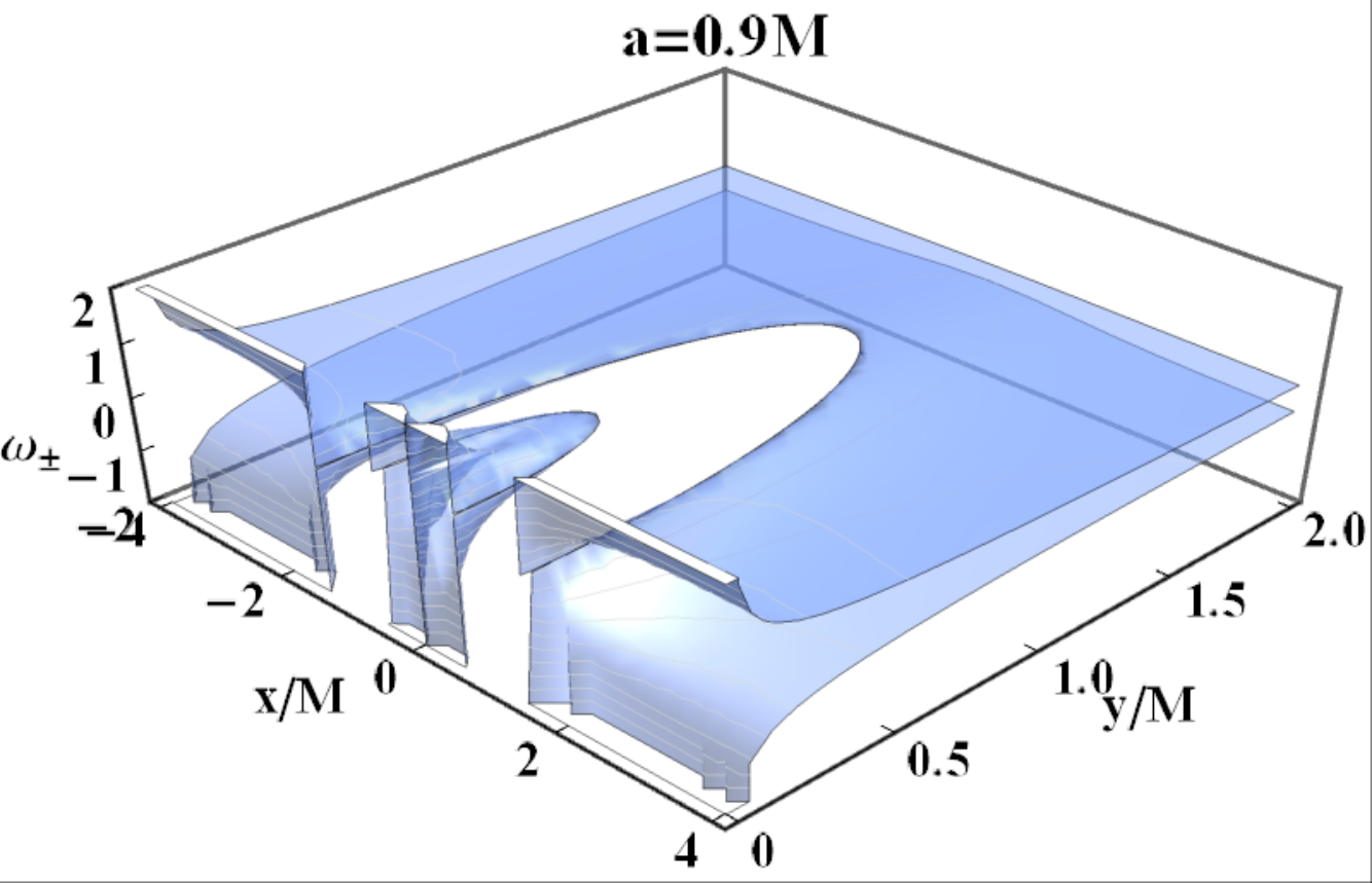
as illustrated in Figs. 1 and 2-right, where the frequencies are plotted for fixed values of and as functions of the spacetime spin and radius , respectively. In particular, the combination
| (9) |
defines null curves, , and, therefore, as we shall see in detail below, the frequencies are limiting angular velocities for physical observers, defining a family of null curves, rotating with the velocity around the axis of symmetry. The Killing vectors are also generators of Killing event horizons. The Killing vector becomes null at r = . At the horizon and, consequently, stationary observers cannot exist inside this surface.
3.1 The frequencies
We are concerned here with the orbits const and const, which are eligible for stationary observers. This analysis enlightens the differences between NS and BH spacetimes. Inside the ergoregion, the quantity in parenthesis in the r.h.s. of Eq. (7) is well defined for any source. However, it becomes null for photon-like particles and the rotational frequencies . On the equatorial plane, the frequencies are given as
| (10) | |||
Moreover, for the case of very strong naked singularities , we obtain that .
The above quantities are closely related to the main black hole characteristics, and determine also the main features that distinguish NS solutions from BH solutions. The constant plays a crucial role for the characterization of black holes, including their thermodynamic properties. It also determines the uniform (rigid) angular velocity on the horizon, representing the fact that the black hole rotates rigidly. This quantity enters directly into the definition of the BH surface gravity and, consequently, into the formulation of the rigidity theorem and into the expressions for the Killing vector (6). More precisely, the Kerr BH surface gravity is defined as , where is the Schwarzschild surface gravity, while (the effective spring constant, according to [111]) is the contribution due to the additional component of the BH intrinsic spin; is therefore the angular velocity (in units of ) on the event horizon. The (strong) rigidity theorem connects then the event horizon with a Killing horizon stating that, under suitable conditions, the event horizon of a stationary (asymptotically flat solution with matter satisfying suitable hyperbolic equations) BH is a Killing horizon99 9 Assuming the cosmic censorship validity, the gravitational collapse should lead to BH configurations. The surface area of the BH event horizon is non-decreasing with time (which is the content of the second law of black hole thermodynamics). The BH event horizon of this stationary solution is a Killing horizon with constant surface gravity (zeroth law) [112, 113, 4, 114]. .
The constant limit plays an important role because it corresponds to the asymptotic limit for very small values of and . Note that, on the equatorial plane, , where . The asymptotic behavior of these frequencies may be deeper investigated by considering the power series expansion for the spin parameter and the radius determined by the expression
| (11) |
which shows a clear decreasing as the gravitational field diminishes. For large values of the rotational parameter, we obtain
| (12) | |||
so that for extreme large values of the source rotation, the frequencies vanish and no stationary observers exist, thought differently for the limiting frequencies (see Figs. 2). It is therefore convenient to introduce the dimensionless radius , for which we obtain the limit
| (13) | |||||
| (14) | |||||
Equations (12), (13) and (14) show the particularly different behavior of with respect to the asymptote . The behavior of the frequencies for fixed values of the radial coordinate and varying values of the specific rotational parameter is illustrated in Fig. 1. We see that the region of allowed values for the frequencies is larger for naked singularities than for black holes. In fact, for certain values of the radial coordinate , stationary observers can exist only in the field of naked singularities. This is a clear indication of the observational differences between black holes and naked singularities.
 |
 
 |
The allowed values for the frequencies are bounded by the limiting value ; for a broader discussion on the role of the dimensionless spin parameter in Kerr geometries, see also [96]1010 10 For simplicity we use here dimensionless quantities. We introduce the rotational version of the Killing vectors and , i.e., the canonical vector fields and . Then, the contraction of the geodesic four-velocity with leads to the (non-conserved) quantity , which is a function of the conserved quantities , the spacetime parameter and the polar coordinate ; on the equatorial plane, it then reduces to . When we consider the principal null congruence , the angular momentum , that is, (and , in proper units), every principal null geodesic is then characterized by . On the horizon, it is [115, 96] Moreover, for a given value of , the corresponding radius is located at a certain distance from the source, depending on the value of the rotational parameter . The following configuration of frequencies, radii and spin determines the location structure of stationary observers:
| (16) | |||
| (17) | |||
Thus, we see that in the interval observers can exist with frequencies ; moreover, the frequency is allowed in , while observers with can exist in . Moreover, it is possible to show that, in BH geometries, the condition must be satisfied outside the outer horizon (). The particular value is therefore the limiting angular velocity in the case of an extreme black hole, i.e., for so that in Eq.(10). The behavior of the special frequency is depicted in Fig. 3 and in Figs. 4, 2, 5, and 6, where other relevant frequencies are also plotted.
 |
Eqs (16) enlighten some important properties of the light surfaces (frequencies ) and of stationary observers, associated with frequencies in the regime of strong singularities. Eqs(16) also enlighten the dependence of the frequencies on the dimensionless spin and radius . It is clear that when the frequency interval shrinks, depending on the singularity spin or the distance from the source , the range of possible frequencies for stationary observers reduces. This occurs in general when . According to Eqs (16), the frequencies are bounded from above by the limiting frequencies and from below by the null value . Thus, at fixed radius , for very strong naked singularities , we have that and the range of possible frequencies for stationary observers becomes smaller. This effect will be discussed more deeply in Sec. 3.2, where we shall focus specifically on the frequency . On the other hand, considering the limits (10), together with Eqs (11)– (), we find that the range of possible frequencies shrinks also in the following situations: when moving outwardly with respect to the singularity (at fixed ), very close to the source, approaching the horizon according to Eq. (10), or also for very large or very small . The last case points out again the importance of the scaled radius .
Essentially, stationary observers can be near the singularity only at a particular frequency. The greater is the NS dimensionless spin, the lower is the limiting frequency , with the extreme limit at . In other words, the frequency range, , for stationary observers vanishes as the value is approached. The singularity at in the NS regime is actually related to the characteristic constant frequency in the same way as in BH-geometries the outer horizon is related to the constant frequency (cf. Eq. (10)). Consequently, a NS solution must be characterized by the frequency and a BH solution by the frequency . Therefore, the frequency may be seen actually as the NS counterpart of the BH horizon angular frequency (see Fig. 4).
 |
 |
 |
 |
 |
For , it holds that .
Then, in general, for BHs and NSs in the static limit , we obtain that
| (18) |
Moreover, for , and inside the ergoregion , while everywhere.
In general, any frequency value should be contained within the range ; therefore, it is convenient to define the frequency interval
| (19) |
which is a function of the radial distance from the source and of the attractor spin. Figs. 7 show the frequency interval as a function of and .
 |
 |
An analysis of this quantity makes it possible to derive some key features about the eligible frequencies. For convenience, we present in Table 1 some special values of the spin-mass ratio, which we will consider in the following analysis. We summarize the obtained results in the following way:
. Black hole classes: Naked singularity classes:
Firstly, for any NS source with , the interval increases as the observer (on the equatorial plane) moves inside the ergoregion towards the static limit.
Secondly, in the case of NS geometries with , i.e., belonging partially to the class of NSI spacetimes, the situation is very articulated. There is a region of maximum and a minimum frequencies, as the observer moves from the source towards the static limit. This phenomenon involves an orbital range partially located within the interval , which is characterized by the presence of counterrotating circular orbits with negative orbital angular momentum (cf. Fig. 8, where the radii are plotted.).
 |
 |
 |
For the maximum spin, , we obtain on the radius and, therefore, the range of possible frequencies for stationary observers vanishes. The points represent the extrema of the interval , i.e., the solutions of the equation – Fig. 8. This property is present only in the case of NS geometries. In fact, there are the two critical orbits and , which are the boundaries of a closed region, whose extension reaches a maximum in the case of the extreme Kerr geometry , and is zero for . For , the separation parameter decreases with the orbital distance, then on the inner radius it reaches a maximum value, whereas on the outer radius it reaches a minimum. In the outer regions, at , the separation parameter increases with the distance from the source. This feature constitutes therefore a major difference in the the behavior of stationary observers within and outside the ergoregion of a naked singularity spacetime. However, a deeper analysis of the equatorial plane, outside the static limit, shows the existence of a second region for light surfaces in the NS case.
On the other hand, the angular velocity decreases with the orbit in the Kerr spacetime. The maximum frequency also decreases in the NS spacetimes. In the BH cases, the angular velocity is always increasing for sources of the class BHI, while for the other sources there is a maximum for the velocity at , which is the circular orbit of a photon or null-like particle corotating with the source. Such a kind of orbit, contained in , is a feature of the BHII-III spacetimes [2], this is also know as marginally or last circular orbit as no circular particle motion is possible in the region . We close this section with a brief discussion on the variation of the frequency interval , following a spin transition with . In the case of a singularity spin-transition, there are two extreme radii for the frequency interval
| (20) | |||
3.2 Light surfaces
In this section, we briefly study the conditions for the existence of light surfaces and and their morphology. The condition (8), for the definition of a stationary observer, can be restated in terms of the solutions , considering as a fixed parameter. Therefore, we now consider the solutions of the equation for the light surfaces defined in Eq. (9) in terms of the Killing null generator , as functions of the frequency . We obtain
| (21) |
where (cf. Eq. (10) and Fig. 2). For , in the limiting case of , we have that and –see Figs. 4, 6 and 21111 11 More precisely, it is for and . Also, for and . In the extreme Kerr spacetime geometry, we have that for , for , and for . For a Kerr geometry, where , it is for or (one positive and one negative value solution), while in the naked singularity case where , the condition is valid only for one negative frequency – see Figs. 5 and 6.. Thus, there are solutions for if where (for simplicity we use a dimensionless spin )
| (22) |
| (23) | |||
| (24) |
The situation is summarized in Table 2.
Black holes: Naked singularities:
We see that for , at1212 12 For a closer look at the role of this special frequency we note that at and, clearly, for . We refer then to Figs. 3, 4, 5, 6, and 9. , at and (the static solution). Moreover, we have that and for BH-sources, where for . In the NS case, there are no crossing points for the radii and (see Fig. 4). The shrinking of the frequency interval is also shown in Figs. 6, 9 and 10, where the radii are also plotted as functions of the frequencies.
 
 |
  |
 |

 |
Figures 4, 5, and 6 contain all the information about the differences between black holes with , and the case of naked singularities with . We summarize the situation in the following statements:
- Naked singularities spacetimes:
-
For , the solutions for the equation of the light surfaces in the limiting case (static observer) are located at . While for any frequency within the range there is one solution , for larger frequencies in the range there are two solutions . In the ergoregion of a naked singularity, there exists a limit for the angular frequency.
- Extreme black hole spacetime:
-
For , we obtain the following set of solutions , , and .
- Black hole spacetimes:
-
We consider first the class BHI with . In the limit , there exists a solution for the light surface with . More generally, the solutions are constrained by the following set of conditions:
(25) (26) (27) Then, we consider BH spacetimes with spin , where . These spacetimes include a part of BHII-sources and the condition applies.
For spacetimes with rotation , the conditions and apply. Then, in the special case or , there is a solution with .
Finally, for spacetimes with , which belong to the class of BHII and BHIII sources, the condition holds, whereas the condition applies for frequencies within the interval . Finally, in the special case , there is one solution at , and for we have the solution .
A summary and comparison of these two cases is proposed also in Figs. 5 and 6, where the surfaces are studied as functions of and . It is evident that the extreme solution is a limiting case of both surfaces , varying both in terms of the spin and the angular velocity . Thus, the difference between the regions where stationary observers can exist in the BH case (gray regions in Figs. 6) and in the NS case are clearly delineated. In BH spacetimes, the surfaces are confined within a restricted radial and frequency range. On the other hand, in the naked singularity case, the orbits and the frequency range is larger than in the black hole case. Moreover, the surfaces can be closed in the case of NS spacetimes, inside the ergoregion, for sufficiently low values of the spin parameter, namely . Furthermore, in any Kerr spacetime, there is a light surface at with . In Sec. 4, we complete this analysis by investigating the special case of zero angular momentum observers, and we find all the spacetime configurations in which they can exist.
4 Zero Angular Momentum Observers
This section is dedicated to the study of Zero Angular Momentum Observers (ZAMOs) which are defined by the condition
| (28) |
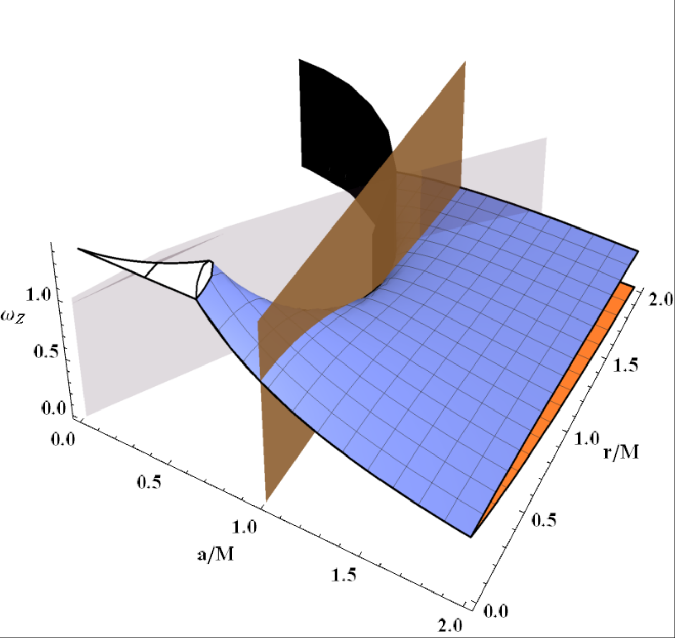
In terms of the particle’s four–velocity, the condition is equivalent to where the quantity is the ZAMOs angular velocity introduced in Eq. (8), and the frequency of arbitrary stationary observers is written in terms of [2]. The sign of is in concordance with the source rotation. The ZAMOs angular velocity is a function of the spacetime spin (see Figs. 11 and 12, where constant ZAMOs frequency profiles are shown). In the plane , we find explicitly
| (29) |
As discussed in [55, 54, 2], ZAMOs along circular orbits with radii are possible only in the case of “slowly rotating” naked singularity spacetimes of class NSI. This is a characteristic of naked singularities which is interpreted generically as a repulsive effect exerted by the singularity [53, 52, 55, 54, 76]. On the other hand, for , while in the region for BH spacetimes, and in the region for NS spacetimes (see also Fig. 12).
ZAMOs angular velocity and orbital regions
The ZAMOs angular velocity is always positive for , and vanishes only in the limiting case . This means that the ZAMOs rotate in the same direction as the source (dragging of inertial frames).
As can be seen from Eq.(29), the frequency for a fixed mass and is strictly decreasing as the radius increases.
For the NS regime it is interesting to investigate the variation of ZAMO frequency on the orbits . These special radii of the NS geometries do not remain constant under a spin-transition of the central singularity. We shall consider this aspect focusing on the curves of the plane as illustrated in Fig. 8. This will enable us to evaluate simultaneously the frequency variation on these special orbits, following a spin variation of the naked singularity in the rage of definition of , and to evaluate the combined effects of a variation in the orbital distance from the singularity and a change of spin. A similar analysis will be done, from a different point of view, also for stationary observers.
In , the velocity (in NSs) always decreases with the orbital radii , i.e. , when the spin increases, i.e. (see Figs. 8 and 12). As monotonically decreases with the spin during a NS spin-up process (see Fig. 8), the frequency decreases in the spin-range , and increases in the range ; therefore, the special value is a minimum point of the ZAMOs frequency – see Fig. 12. Viceversa, as increases after a NS spin-up, the corresponding ZAMOs frequency decreases as the observer moves along the curve . Thus, we can say that, if the NS spin increases, the frequency decreases, approaching, but never reaching, the singularity, i. e., for . Viceversa, increasing the NSs spin in spacetimes with , the frequency increases again and the orbit moves towards the central singularity. On the other hand, the frequency monotonically decreases with the naked singularity spin, i.e. ; therefore, for a fixed NS spin, the frequency interval decreases, i.e. . In fact, the velocity is strictly decreasing with the radius in the BH and NS regimes with (i.e. ). Moreover, in general increases as the observer approaches the black hole at fixed spin, and it decreases as the observer moves far away from the center of rotation.
In the static limit, we have that . In fact, the asymptotic behavior of the frequency is determined by the relations
| (30) |
Change in the intrinsic spin The angular velocity of the ZAMOs inside varies according to the source spin. This might be especially important in a possible process of spin-up or spin-down as a result of the interaction, for example, with the surrounding matter. In [2], this phenomenon and its implications were investigated, considering different regions close to the singularity. For a fixed orbital radius , the ZAMOs angular velocity strongly depends on the value of the spacetime spin-mass ratio. In particular, depending on the value of the ratio , there can exist a radius of maximum frequency given by
| (31) |
that are solutions of the equation at which the frequency is denoted by (see Figs. 11 and 12). A detailed analysis of the expression for the radius shows that in can exist in spacetimes that belong to the class BHII with spin , where , and to the classes BHIII, NSI, and NSII with the limiting value , where (see Figs. 11 and 2). Spacetimes with spin belong to the class BHII, as defined in Table 2, and have been analyzed in the context of stationary observers in Sec. 3.2 and Sec. 3.1 (Figs. 4, 11, 12 and 13 show the behavior of several quantities related to ZAMOs in relation to other frequencies.). In this particular case, we have that
| (32) |
We focus our attention on ergoregion , bounded from above by the radius and from below by and for NSs and BHs, respectively. We consider the role of the radius , as the maximum point of the ZAMO frequency, as a function of the source spin-mass ratio. Thus, for black holes with , the frequency increases with always inside the ergoregion; this holds for any orbit inside (i.e. for a fixed value , if a BH spin-up shift occurs in the range , the function increases with ). For spins , instead, the frequency grows with the spin only for ; on the contrary, for radii located close to the horizon, , decreases following a spin up in the range (i.e, and ). In the case of NS-spacetimes, the frequency is an increasing function of the dimensionless spin in the NS spin range and on the orbit . Moreover, the frequency decreases with the spin in the range of values and on . This situation is distinctly different for NS with , for which in the ergoregion an increase of the spin corresponds to a decrease of . This is an important distinction between different NS regimes.
We note that for the spin (see Fig. 11). Moreover, in naked singularity spacetimes with spin , we obtain that –Fig. 12. Remarkably, the spin is the maximum point of the frequency and also the maximum point of the frequency (see Fig. 2). In other words, in naked singularity spacetimes with , where , the ZAMOs frequency at the ergosurface reaches a maximum value which is equal to , defined through the radius in Eq. (31); moreover, the frequency reaches its maximum value at the ergosurface.
 |
 |
 |
 |
ZAMOs energy
The circular motion of test particles can be described easily by using the effective potential approach [116]. The exact form of such an effective potential in the Kerr spacetime is well known in the literature (see, for example, [55, 54]). The effective potential function represents the value of that makes into a turning point , being the particle mass; in other words, it is the value of (in the case of photons, shall depend on an affine parameter and the impact parameter is relevant for the analysis of trajectories) at which the (radial) kinetic energy of the particle vanishes. This can easily be obtained from the geodesic equations with the appropriate constraints or through the normalization conditions of the four-velocities, taking into account the constraints and the constants of motion [116]. Here we consider specifically an effective potential associated to the ZAMOs.
The orbits are critical points of the effective potential, i. e., . Here we consider for the ZAMO where is a factor related to the normalization condition of the ZAMO four-velocity ( for timelike ZAMOs, where and , according to Eq. (3); in the ergoregion , but for and ). The energy of the ZAMOs is always positive for both BH and NS spacetimes, and it grows with the source spin; in fact, solutions for are not possible because this would correspond to the case of a null angular momentum with null energy. The energy on the orbits where is always positive. In BH geometries, the potential , at , increases with the distance from the source and has no critical points as a function of . The most interesting case is then for the slow naked singularity spacetimes of the first class, NSI with , where there is a closed and connected orbital region of circular orbits with . The radii are ZAMOs orbits, and in this region the potential decreases with the orbital radius. However, in the outer region , the potential increases with the radius. This implies that the radii are possible circular ZAMOs orbits. In fact, is an unstable orbit and is a stable orbit. Thus, in any geometry of this set, there is a stable orbit for the ZAMOs with angular velocity different from zero, where (see Fig. 12).
In [2], we investigated the orbital nature of the static limit. Here, in Fig. 13, the velocity and the ratio (that is, the inverse of the specific angular momentum defined as ) are considered as functions of the source spin at the static limit. We explore the relation between the ZAMOs and the stationary observes, where , for NSI sources at the static limit. A maximum value, , is reached at . Also, a maximum value exists for the ZAMOs angular velocity at . This ratio is always greater than the angular momentum of the ZAMOs at the static limit.
In BH spacetimes, the angular velocity for stationary observers is limited by the value which occurs for the radius . We can evaluate the deviation of this velocity in a neighborhood of the radius , since the four-velocity of the observers rotating with (where ) must be timelike outside the horizon and therefore it has to be in that range (the event horizon of a Kerr black hole rotates with angular velocity [1]). This limit cannot be extended to the case of naked singularities. However, one can set similarly the threshold in the case of circular orbits, where the frequency limit is restricted to the values as .
 |
 |
5 Summary and Conclusions
In this work, we carried out a detailed analysis of the physical properties of stationary observers moving in the ergoregion along equatorial circular orbits in the gravitational field of a spinning source, described by the stationary and axisymmetric Kerr metric. We derived the explicit value of the angular velocity of stationary observers and analyzed all possible regions where circular motion is allowed, depending on the radius and the rotational Kerr parameter. We found that in general the region of allowed values for the frequencies is larger for naked singularities than for black holes. In fact, for certain values of the radius , stationary observers can exist only in the field of naked singularities. We interpret this result as a clear indication of the observational differences between black holes and naked singularities. Given the frequency and the orbit radius of a stationary observer, it is always possible to determine the value of the rotational parameter of the gravitational source. Our results show that in fact the probability of existence of a stationary observer is greater in the case of naked singularities that in the case of black holes. Moreover, it is possible to introduce a classification of rotating sources by using their rotational parameter which, in turn, determines the properties of stationary observers. Black holes and naked singularities turn out to be split each into three different classes in which stationary observers with different properties can exist. In particular, we point out the existence of weak (NSI) and strong (NSIII) naked singularities, corresponding to spin values close to or distant from the limiting case of an extreme black hole, respectively.
Light surfaces are also a common feature of rotating gravitational configurations. We derived the explicit value of the radius for light surfaces on the equatorial plane of the Kerr spacetime. In the case of black holes, light surfaces are confined within a restricted radial and frequency range. On the contrary, in the naked singularity case, the orbits and the frequency ranges are larger than for black holes. Again, we conclude that light surfaces can be found more often in naked singularities. The observation and measurement of the physical parameters of a particular light surface is sufficient to determine the main rotational properties of the spinning gravitational source. We believe that the study of light surfaces (defining the “throat” discussed in Sec. 3) has important applications regarding the possibility of directly observing a black hole in the immediate vicinity of an event horizon (within the region defined by the static limit), as this seems to be possible in the immediate future through, for example, the already active Event Horizon Telescope (EHT) projects1313 13 http://www.eventhorizontelescope.org/.
We also analyzed the conditions under which a ZAMO can exist in a Kerr spacetime. In particular, we computed the orbital regions and the energy of ZAMOs. The frequency of the ZAMOs is always positive, i.e., they rotate in the same direction of the spinning source as a consequence of the dragging of inertial frames. The energy is also always positive. The most interesting case is that of slowly rotating naked singularities (NSI) where there exists a closed and disconnected orbital region. This particular property could, in principle, be used to detect naked singularities of this class. We derived the particular radius at which the frequency of the ZAMOs is maximal, showing that the measurement of this radius could be used to determine whether the spinning source is a black hole or a naked singularity and its class, according to the classification scheme formulated here. To be more specific, from Table 2 we infer that the existence of stationary observers in black hole spacetimes is limited from above by the frequency , which is the highest frequency on the static limit, implying the frequency lower bound – see also Fig. 4. In this figure, we also show the maximum frequency, , at the static limit for a naked singularity with . This spin plays an important role for the variation of the ZAMOs frequency in NSs in terms of the singularity dimensionless spin – see Fig. 12 and Fig. 13. On the other hand, for strong BHs, with , the frequency is bounded from below by and from above by , as the radial upper bound is . A similar situation occurs for NSs, provided that is replaced with the limiting frequency . The special role of the BH spin is related to the presence of the photon circular orbit in the BH ergoregion, which is absent in NS geometries; consequently, as seen in Table 2, there is no distinction between the naked singularities classes. However, the analysis of the frequencies in Fig. 4 shows differently that there are indeed distinguishing features in the corresponding ergoregions. In the case of naked singularities, the frequency range of stationary observers has as a boundary the outer light-surface, , then it narrows as the spin increases, and finally vanishes near the static limit.
The frequency of the orbits on the static limit, in fact, converges to the limit , which is an important frequency threshold for the NS regime. The presence of a maximum for the special NS geometry with on the static limit is symptomatic for the nature of this source – see Figs. 4, 6 and 13. The study of the surfaces on the plane , for different values of the spin-mass ratio, shows a clear difference between the allowed regions in naked singularities and black holes (gray region in Fig. 6). There is an open “throat” between the spin values (strong BHs) and (very weak NSs), with an opening of the cusp (at in these special coordinates) for the frequency . We note a change in the situation for spins in ; this region is in fact extremely sensitive to a change of the source spin; the throat of has, in this special spin range, a saddle point around between , which is not present in stronger singularities. The spins in this range are related to the negative state energy and the radii , where the orbital energy is – Fig. 8. Particularly, we point out the spin , where , for which at there is a critical point of the frequency amplitude . In BH geometries, the frequencies increase with the spin and with the decrease of the radius towards the horizon. The curves continue to increase with the presence of a transition throat at that increases, stretching and widening. This throat represents a “transition region” between BH and super-spinning sources from the viewpoint of stationary observes. The regions outlined here play a distinct role in the collapse processes with possible spin oscillations and different behaviors for weak, very weak, and strong naked singularities. As the spin increases, the frequencies of NSs observes move to lower values, widening the throat. This trend, however, changes with the spin, enlightening some special thresholds.
This analysis shows firstly the importance of the limiting frequency , determining the main properties of both frequencies and the radii ; it is also relevant in relation to ZAMOs dynamics in NS geometries. In this way, we may see as an extension of the frequency at the horizon for BH solutions–Fig. 4. In the NS regime, all the curves converge to the same “focal point” , regardless of the type of naked singularity, but as is the limiting frequency at the BH horizon, each source is characterized by only one frequency. The greater is the spin, the lower is the frequency at fixed radius, and particularly in the neighborhood of the singularity ring, according to the limiting value . The frequency range at fixed narrows for higher dimensionless NS spin . This feature distinguishes between strong, weak and very weak naked singularities. From Figs. 6 it is clear also that the throat of the light-surfaces , in the plane , for different spins closes for , which is a spin transition region that includes the extreme Kerr solution. This region has been enlarged in Fig. 6-bottom. Figures 9 and 10 show from a different perspective the transition between the BH region, gray region in Figs. 6, and the NS region for different spins. Any spin oscillation in that region generates a tunnel in the light-surface1414 14 Since any simulation of stellar collapse returns to the BH regime, there must be some (retroactive) mechanism that closes the observer tunnel, as even light does not run away in the forbidden region at . Moreover, hypothetical super-luminary matter would violate the bonding of the tunnel wall.. The transition region is around , which is a special value related to the spin of strong naked singularities–see Figs. 3 and 2. In this region, as in the neighborhood of the ring singularity , the orbital range reaches relatively small values1515 15 It is worth to mention that predicted quantum effects close to the singularities could play a major role in this region. However, we recall that the extreme limit in this model is never faced, as we continue to see the spacetime for all NSs using a Boyer-Lindquist frame. It is well known that approaching the horizon at , the radial coordinate velocity appears as never penetrating the black hole, spiraling as goes to infinity. This is the consequence of a coordinate singularity which can be avoided by using Kerr coordinates or Eddington-Finkelstein coordinates.. This shows the existence of limitations for a spin transition in the parameter region of very weak naked singularities, pointed out also in [53, 52, 76, 54, 55].
On the other hand, in the strong NSs regimes, a spin threshold emerges at and (see Figs. 3, 4 and 6). In Fig. 13, we analyze the properties at the static limit . The maximum value of is then reached in the ergoregion of the NSII class1616 16 The throat depth in the region would lead to an immediate change of the observers properties and it is reasonable to ask if this may imply an activation instead of a “positive feedback” phenomenon. We recall that in this scenario, we are not considering a change of symmetries which would have an essential role. Then it is important to emphasize that in these hypothetical spin transitions, the external boundary of the ergoregion remains unchanged, but not the frequency at the static limit.. Around the throat width becomes more or less constant. The situation is different for and and then for , where the frequencies range narrows, and near becomes restricted to a small range of a few mass units in the limit of large spin . In strong and very strong NSs, the wide region is inaccessible for stationary observers, whereas it is accessible in the BH case. This significantly separates strong and weak NSs, and distinguish them from the BH case. Interestingly, the saddle point around , which narrows the throat of frequencies even in the case of NS geometries for , could perhaps be viewed as a trace of the presence of , which is absent for . For , where the saddle point disappears, the shape of the tube is different. This, on the other hand, would suggest that the existence of the flex in the case of very weak NSs would prevent a further increasing of the spin. This does not hold for a transition to stronger NSs, , where no saddle point is present–Fig. 8-bottom. Obviously, the consequences of the hypothetical transition processes should also take into account the transient phase times. Very weak naked singularities show a “rippled-structure” in the frequency profiles of with respect to and , as appears in Figs. 2, 6, 9, and 10. The significance of this structure is still to be fully investigated, but it may be seen perhaps as a fingerprint-remnant of the BH horizon. This may open an interesting perspective for the study of NS geometries.
An interesting application of our results would be related to the characterization of the optical phenomena in the Kerr naked singularity and black hole geometries, such as the BH raytracing and the determination of the BH silhouette (shadow). The light escape cones are a key element for such phenomena. Light escape cones of local observers (intended as sources) determine the portion of radiation emitted by a source that could escape to infinity and the one which is trapped. This is related to the study of the radial motion of photons because the boundary of the escape cones is given by directional angles associated to unstable spherical photon orbits. Light escape cones can be identified in locally non-rotating frames, in frames associated to circular geodesic motion and in radially free-falling observers [117, 118, 42, 119, 120]. We want to point out, however, that light escape cones do not define the properties of the light-cone causal structure, and are not directly related to stationary observers; they rather depend on the photon orbits. A thoroughout analysis of the photon circular motion in the region of the ergoregion can be found in [2]. In Figs. 1, 3, 4 and 12, we show the photon orbit and the limiting frequencies crossing this radius; this enlightens the relation with the frequency . We consider there in more detail the relation between the quantities , the constants of motion and and the effective potential, briefly addressed also in Sec. 4.
In general, we see that it is possible to detect black holes and naked singularities by analyzing the physical properties (orbital radius and frequency) of stationary observers and ZAMOs. Moreover, the main physical properties (mass and angular momentum) of the spinning gravitational source can be determined by measuring the parameters of stationary observers. This is certainly important for astrophysical purposes since the detection and analysis of compact astrophysical objects is one of the most important issues of modern relativistic astrophysics. In addition, the results presented in this work are relevant especially for investigating non-isolated singularities, the energy extraction processes, according to Penrose mechanism, and the gravitational collapse processes which lead to the formation of black holes.
Acknowledgements.
D.P. acknowledges support from the Junior GACR grant of the Czech Science Foundation No:16-03564Y. This work was partially supported by UNAM-DGAPA-PAPIIT, Grant No. 111617. D.P. thanks Dr. Jan Schee for interesting discussion on the light escape cone and stationary observers.References
- (1) R. M. Wald, General Relativity, (The University of Chicago Press, Chicago, 1984).
- (2) D. Pugliese & H. Quevedo, Eur. Phys. J. C 75, 5, 234 (2015).
- (3) J. D. Bekenstein, Phys. Rev. D 7, 2333 (1973).
- (4) R. M. Wald, Living Rev. Relativ. 4(1), 6 (2001).
- (5) T. M. Fiola, J. Preskill, A. Strominger and S. P. Trivedi, Phys. Rev. D 50, 3987 (1994).
- (6) H. Nikolic, Phys. Lett. B 678, 218 (2009).
- (7) K. Bradler & C. Adami, JHEP 1405, 095 (2014).
- (8) L. Susskind, Scientific American 276, 4, 52-57 (1997).
- (9) S.W.Hawking, Comm. Math. Phys. 43, 199 (1975) Erratum - ibidem 46, 206 (1976).
- (10) S.W.Hawing, Mon. Not. R. astr. Soc.152, 75-78 (1971).
- (11) R. Penrose, Revista del Nuovo Cimento (1969).
- (12) J.D. Bekenstein, Phys. Rev. D, 12, 3077 (1975).
- (13) R. Penrose, and R. M. Floyd, Science 229, 177179 (1971).
- (14) F. Gray, S. Schuster, A. VanBrunt and M. Visser, Class. Quant. Grav. 33, 11, 115003, (2016).
- (15) M. Bejger, T. Piran, M. Abramowicz and F. Hakanson, Phys. Rev. Lett. 109, 121101 (2012).
- (16) Z. Stuchlik, P. Slany, G. Torok and M. A. Abramowicz, Phys. Rev. D 71, 024037 (2005).
- (17) D. L. Meier, Black Hole Astrophysics The Engine Paradigm, (Springer-Verlag, Berlin Heidelberg, 2012).
- (18) V. P. Frolov, A. Zelnikov, Introduction to Black Hole Physics, (Oxford University Press, 488, 2011).
- (19) J. Gariel, G. Marcilhacy and N. O. Santos, Astrophys. J. 774, 109 (2013).
- (20) R. Znajek, Nature, 262, 270 (1976).
- (21) A. R. Prasanna and R. K. Varma, Pramana 8, 3 229 (1977).
- (22) A. R. Prasanna and C. V. Vishveshwara, Pramana 11, 359 (1978).
- (23) A. N. Aliev and N. Özdemir, Mon. Not. Roy. Astron. Soc. 336, 241 (2002).
- (24) G. Preti, Class. Quantum Grav. 21, 3433 (2004).
- (25) P. Bakala, E. Šrámková, Z. Stuchlík, and G. Török, Class. Quantum Grav. 27, 045001 (2010).
- (26) V. P. Frolov and A. A. Shoom, Phys. Rev. D 82, 084034 (2010).
- (27) T. Igata, T. Harada, M. Kimura, Phys.Rev. D 85, 104028 (2012).
- (28) R. Shiose, M. Kimura, T. Chiba, Phys. Rev. D 90, 124016 (2014).
- (29) S. Hussain, I. Hussain, M. Jamil, Eur. Phys. J. C 74 12, 3210 (2014).
- (30) G. Pei, S. Nampalliwar, C. Bambi and M. J. Middleton, Eur. Phys. J. C 76, 10, 534 (2016).
- (31) S. S. Komissarov, J. Korean Phys. Soc. 54, 2503 (2009).
- (32) J.-P. Lasota, E. Gourgoulhon, M. Abramowicz, A. Tchekhovskoy and R. Narayan, Phys. Rev. D 89, 2, 024041 (2014).
- (33) Z. Stuchlik & J. Kovar, Class. Quant. Grav. 23, 3935 (2006).
- (34) Z. Stuchlik, D. Pugliese, J. Schee and H. Kucáková, Eur. Phys. J. C 75, 9, 451 (2015).
- (35) A. Kotrlová, G. Török, E. Sramková & Z. Stuchlík, A&A 572, A79 (2014).
- (36) K. Boshkayev, E. Gasperín, A.C. Gutiérrez-Piñeres, H. Quevedo, & S. Toktarbay Phys. Rev. D 93, 024024 (2015).
- (37) M. Kolos & Z. Stuchlík, Phys. Rev. D 88 065004, (2013).
- (38) J. Schee & Z. Stuchlik, JCAP 1304, 005 (2013).
- (39) G. Torok & Z. Stuchlik, Astron. Astrophys. 437, 775 (2005).
- (40) Z. Stuchlik, Bull. Astron. Inst. Czech, 32, 2, 68-72 (1981).
- (41) Z. Stuchlík, S. Hledík, K. Truparová, Class. Quant. Grav. 28, 15 155017 (2011).
- (42) Z. Stuchlik & J. Schee, Class. Quant. Grav. 27, 215017 (2010).
- (43) M. Patil & P. S. Joshi, Class. Quant. Grav. 28, 235012 (2011).
- (44) Z. Stuchlik & J. Schee, Class. Quant. Grav. 29 065002, (2012).
- (45) Z. Stuchlik & J. Schee, Class. Quant. Grav. 30, 075012 (2013).
- (46) K. I. Nakao, P. S. Joshi, J. Q. Guo, P. Kocherlakota, H. Tagoshi, T. Harada, M. Patil and A. Krolak, arXiv:1707.07242 [gr-qc].
- (47) M. J. Lake & B. Carr, JHEP 1511, 105 (2015).
- (48) B. J. Carr, arXiv:1703.08655 [gr-qc].
- (49) B. J. Carr, J. Mureika and P. Nicolini, JHEP 1507, 052 (2015).
- (50) B. J. Carr, Springer Proc. Phys. 170, 159 (2016).
- (51) Y. Prok et al. [CLAS Collaboration], Phys. Lett. B 672 (2009) 12
- (52) D. Pugliese, H. Quevedo and R. Ruffini, Eur. Phys. J. C 77, 4, 206 (2017).
- (53) D. Pugliese, H. Quevedo and R. Ruffini, Phys. Rev. D 83, 104052 (2011).
- (54) D. Pugliese, H. Quevedo and R. Ruffini, Phys. Rev. D 88, 024042 (2013).
- (55) D. Pugliese, H. Quevedo and R. Ruffini, Phys. Rev. D 84, 044030 (2011).
- (56) R. Goswami, P. S. Joshi and P. Singh, Phys. Rev. Lett. 96, 031302 (2006).
- (57) C. Vaz & L. Witten, Phys. Lett. B 442, 90 (1998).
- (58) H. Iguchi, T. Harada and K. i. Nakao, Prog. Theor. Phys. 101, 1235 (1999).
- (59) H. Iguchi, K. i. Nakao and T. Harada, Phys. Rev. D 57, 7262 (1998).
- (60) H. Iguchi, T. Harada and K. I. Nakao, Prog. Theor. Phys. 103, 53 (2000).
- (61) S. L. Shapiro & S. A. Teukolsky, Phys. Rev. Lett. 66, 994 (1991).
- (62) T. A. Apostolatos & K. S. Thorne,Phys. Rev. D 46, 2435 (1992).
- (63) T. Jacobson& T. P. Sotiriou, Phys. Rev. Lett. 103, 141101 (2009).
- (64) T. Jacobson & T. P. Sotiriou, J. Phys. Conf. Ser. 222, 012041 (2010).
- (65) E. Barausse, V. Cardoso, and G. Khanna. Phys. Rev. Lett. 105, 261102 (2010).
- (66) B. Giacomazzo, L. Rezzolla and N. Stergioulas, Phys. Rev. D 84, 024022 (2011).
- (67) V. Cardoso, P. Pani, M. Cadoni and M. Cavaglia, Phys. Rev. D 77, 124 044 (2008).
- (68) N. Comins & B. F. Schutz, Proc. R. Soc. A 364, 1717 211-226 (1978).
- (69) A. Helou, I. Musco and J. C. Miller, arXiv:1601.05109 [gr-qc].
- (70) R. M. Wald & V. Iyer, Phys. Rev. D 44, 3719 (1991).
- (71) P. S. Joshi, Gravitational Collapse and Spacetime Singularities , Cambridge Monographs on Mathematical Physics, New York 2007.
- (72) B. P. Abbott et al. (LIGO Scientific Collaboration and Virgo Collaboration) Phys. Rev. Lett. 116, 061102 (2016).
- (73) B. P. Abbott et al. [LIGO Scientific and Virgo Collaborations], Phys. Rev. Lett. 119, 16, 161101 (2017).
- (74) B. P. Abbott et al. [LIGO Scientific and Virgo and Fermi-GBM and INTEGRAL Collaborations], Astrophys. J. 848, 2, L13 (2017).
- (75) M. Blaschke & Z. Stuchlík, Phys. Rev. D 94, 8, 086006 (2016).
- (76) D. Pugliese, H. Quevedo and R. Ruffini, Phys. Rev. D 83, 024021 (2011).
- (77) D. B. Malament, J. Math. Phys., 18, 1399 (1977).
- (78) S. W. Hawking, A. R. King, and P. J. McCarthy, J. Math. Phys., 17, 174 (1976)
- (79) R. P. Geroch, J. Math. Phys., 8, 782 (1967)
- (80) F. de Felice, A&A 34, 15 (1974).
- (81) F. de Felice, Nature 273, 429-431 (1978).
- (82) Z. Stuchlík & J. Schee, Int. J. Mod. Phys. D 24, 1550020 (2015).
- (83) J. Schee & Z. Stuchlik, JCAP 1506 048, (2015).
- (84) J. Gariel, N. O. Santos and J. Silk, Phys. Rev. D 90, 063505 (2014).
- (85) N. Pelavas, N. Neary and K. Lake, Class. Quant. Grav. 18, 1319 (2001).
- (86) C. Herdeiro & E. Radu, Phys. Rev. D 89, 124018 (2014).
- (87) Z. Stuchlik, Bull. Astron. Inst. Czech 31, 129 (1980).
- (88) S. Gao & Y. Zhang, Phys. Rev. D 87, 4 044028 (2013).
- (89) Z. Stuchlik, S. Hledik and K. Truparova, Class. Quant. Grav. 28, 155017 (2011).
- (90) M. H. P. M. van Putten, Prog. Theor. Phys. 127, 2 331-354 (2012).
- (91) C. F. Gammie, S. L. Shapiro and J. C. McKinney, Astrophys. J. 602, 312 (2004).
- (92) P. Abolmasov Mon. Not. R. Astron. Soc. 432, 761-768 (2013).
- (93) M. Kesden, Phys. Rev. D 83, 104011 (2011).
- (94) R. M. Wald, Ann. Phys. 82, 548 (1974).
- (95) P. Pradhan & P. Majumdar, Eur. Phys. J. C 73, 6 2470 (2013).
- (96) D. Pugliese & G. Montani, Phys. Rev. D 91, 8, 083011 (2015).
- (97) D. Pugliese & Z. Stuchlik, Astrophys. J. Suppl. 221, 25 (2015).
- (98) D. Pugliese & Z. Stuchlik, Astrophys. J. Suppl. 229, 2, 40 (2017).
- (99) D. Pugliese & Z. Stuchlik, Astrophys. J. Suppl. 223, 2, 27 (2016).
- (100) D. Pugliese & Z. Stuchlik, JHEAp 17, 1 (2018).
- (101) Z. Li & C. Bambi, Phys. Rev. D 87, 124022 (2013).
- (102) J. Biéak, Z. Stuchlík, and V. Balek, Bull. Astron. Inst. Czech 40, 2 65-92 (1989).
- (103) V. Balek, J.Bicak, Z. Stuchlik, Bull. Astron. Inst. Czech 40, 3 133-165 (1989).
- (104) J. Kovar, O. Kopacek, V. Karas and Z. Stuchlik, Class. Quant. Grav. 27, 135006 (2010).
- (105) S. W. Hawking & G. F. R. Ellis, The large scale structure of space-time, (Cambridge University Press, Cambridge, 1973).
- (106) C. Chakraborty, M. Patil, P. Kocherlakota, S. Bhattacharyya, P. S. Joshi and A. Krolak, Phys. Rev. D 95, 8, 084024 (2017).
- (107) A. V. Frolov & V. P. Frolov, Phys. Rev. D 90, 12, 124010 (2014).
- (108) J. B. Griffiths & J. Podolský, Exact space-times in Einstein’s General Relativity, (Cambridge University Press, Cambridge, 2009).
- (109) L.D. Landau& E.M. Lifshitz, The Classical Theory of Fields, (Oxford, Pergamon Press, 1980).
- (110) E. Poisson, A Relativist’s Toolkit: The Mathematics of Black-Hole Mechanics, 1st Edition 2004, Cambridge University Press.
- (111) M. R. R. Good & Y. C. Ong, Phys. Rev. D 91, 4, 044031 (2015).
- (112) P. T. Chrusciel, J. Lopes Costa and M. Heusler, Living Rev. Rel. 15, 7 (2012).
- (113) B. Carter, gr-qc/9712038.
- (114) R. M. Wald, Class. Quant. Grav. 16, A177 (1999).
- (115) S. Chandrasekhar, The Mathematical Theory of Black Holes, Oxford University Press (1983).
- (116) C. W. Misner, K. S. Thorne, J. A. Wheeler, Gravitation, (Freeman, San Francisco, 1973).
- (117) J. Schee, Z. Stuchlik & J. Juran, Proceedings of RAGtime 6/7: Workshops on black holes and neutron stars, Opava, 16-18/18-20 September, 2004/2005
- (118) J. Schee & Z. Stuchlik, Int. J. Mod. Phys. D 18, 983 (2009).
- (119) R. Takahashi, M. Takahashi, A&A, 513, A77, 7 (2010).
- (120) J. Schee & Z. Stuchlik, Gen. Rel. Grav. 41, 1795 (2009).