Pair-cat codes: autonomous error-correction with low-order nonlinearity
Abstract
We introduce a driven-dissipative two-mode bosonic system whose reservoir causes simultaneous loss of two photons in each mode and whose steady states are superpositions of pair-coherent/Barut-Girardello coherent states. We show how quantum information encoded in a steady-state subspace of this system is exponentially immune to phase drifts (cavity dephasing) in both modes. Additionally, it is possible to protect information from arbitrary photon loss in either (but not simultaneously both) of the modes by continuously monitoring the difference between the expected photon numbers of the logical states. Despite employing more resources, the two-mode scheme enjoys two advantages over its one-mode cat-qubit counterpart with regards to implementation using current circuit QED technology. First, monitoring the photon number difference can be done without turning off the currently implementable dissipative stabilizing process. Second, a lower average photon number per mode is required to enjoy a level of protection at least as good as that of the cat-codes. We discuss circuit QED proposals to stabilize the code states, perform gates, and protect against photon loss via either active syndrome measurement or an autonomous procedure. We introduce quasiprobability distributions allowing us to represent two-mode states of fixed photon number difference in a two-dimensional complex plane, instead of the full four-dimensional two-mode phase space. The two-mode codes are generalized to multiple modes in an extension of the stabilizer formalism to non-diagonalizable stabilizers. The -mode codes can protect against either arbitrary photon losses in up to modes or arbitrary losses and gains in any one mode.
Keywords:
continuous variable quantum information, Wigner function, cat code, error correction, stabilizer formalismI Introduction
I.1 Motivation & outline
The search for how to realize the first fault-tolerant quantum computer is currently underway. Due to the fragility of quantum information, one has to encode said information redundantly into physical degrees of freedom in order to be able to protect it from noise. In the field of continuous-variable (CV) quantum information processing [1, 2, 3, 4], one encodes information in the space corresponding to the occupation (photon) number of a harmonic oscillator. A CV quantum code is then a subspace of the oscillator Hilbert space that is used to protect quantum information against errors.
Beginning with the two-mode “dual-rail” encoding in 1995 [5], there are currently several CV codes on the market. One can characterize them by the oscillator basis states that most conveniently expresses the code: Fock/number states [6, 7, 8, 9, 10, 11, 12], position and momentum eigenstates and [13, 14, 15, 16, 17, 18], or a few coherent states (for some finite set ) [19, 20, 21, 22]. There also exist hybrid schemes which couple an oscillator to other systems [23, 24]. In addition to the continuing focus on optical cavity implementations, a few of the recent efforts [21, 11, 12] are tailoring codes for use in microwave cavities (modes) coupled to Josephson junctions [25, 26]. In particular, a class of single-mode codes known as the cat codes [19, 21] (see also [27, 28, 29, 30]) has enjoyed rapid experimental progress in the microwave paradigm [31, 32, 33] and may be applicable to protect against dephasing in phononic systems [34, 35]. It is thus natural to consider similarly-tailored generalizations of this class to multiple modes.
In this manuscript, we present both a new code family — the pair-cat codes — and a proposal for its realization using reservoir-engineered (a term coined in Ref. [36]) microwave cavities. We show that the pair-cat code offers a promising balance between protection from errors and near-term realizability. Namely, it is tailored to protect from the largest incoherent source of error of microwave cavities — photon loss — and its implementation provides several advantages over previous designs.
Let be a dissipator [37, 38, 39],
| (1) |
where is a jump operator and a density matrix. We consider two schemes with respective jump operators
| (2a) | |||||
| (2b) | |||||
Above, are the two oscillator mode operators, but we also use them to label the modes, and are complex parameters. The modes obey the standard commutation relations and and we denote photon number operators and . Storage of at least a qubit worth of information as well as suppression of error processes requires a certain degree of symmetry, which is main reason for why are high-order (quartic) processes. Scheme I has already been thoroughly studied [21, 27] and we only review it here in a context that allows for a direct analogy with the new scheme II.
Time evolution of a one- or two-mode density matrix is then governed by the Lindbladian
| (3) |
where and corresponds to jump the respective operators in Eq. (2a-b), is a non-negative rate and “” represent competing error processes. The competing error processes include loss errors, caused by dissipators of the form and , and dephasing errors, caused by dissipators of the form and . Quantum information is encoded in certain steady states of , i.e., states such that , which form a decoherence-free subspace of [40, 41, 42], represented by its projection . In the cases considered here, the code subspace satisfies , meaning that annihilates all states that are in the subspace (i.e., all states for which ).
We continue this section by discussing the advantages of scheme II and describing how to analyze errors and gates for both schemes. In Sec. II, we review code properties and gates for scheme I. In Sec. III, we do the same for scheme II. In Sec. IV, we introduce techniques to visualize two-mode states in a two-dimensional plane. In Sec. V, we comment on multimode generalizations and make contact with the stabilizer formalism. In Sec. VI, we develop the experimental realization for scheme II. We conclude in Sec. IX.
I.2 Advantages of pair-cat codes
In this work, we introduce a complete error-correction method for the two-mode scheme II. A side-by-side comparison to scheme I is in Table 1. The leading uncorrectable errors for both schemes are of the same order, for scheme I and for scheme II, so the code subspaces in both schemes are of comparable quality. However, while retaining all of the benefits of the cat codes, scheme II enjoys several advantages, including most importantly a drastic reduction of the order of the nonlinearity required for realization. Three- and higher-mode extensions of scheme II further increase the error-correcting properties of the codes, e.g., an -mode code for enjoys a leading-order uncorrectable loss error of . We summarize these advantages below.
I.2.1 Discrete QEC against photon loss
One can show that a dominant dissipative term (3) is able to continuously suppress (or, in the sense of Ref. [43], passively protect from) any dephasing error processes without the need for error syndrome measurement and recovery operations. In this work, we refer to an error-correction process that is continuous in time and that does not require active measurement and feedback operations as continuous quantum error correction (QEC) [44, 45, 46, 47, 48, 49, 50, 51, 24, 52].11 1 Continuous means “continuous in time” and autonomous means “without measurement and feedback” [53], but we use the terms interchangeably since all of our continuous QEC is also autonomous. Both schemes also admit discrete QEC (i.e., conventional protection via non-demolition measurements of error syndromes and adaptive control) against photon loss, but only scheme II can perform both QEC processes simultaneously using currently available techniques.
The scheme I syndrome is the photon number parity,
| (4) |
and parity measurements [54] and full-blown discrete QEC [32] for scheme I have been implemented using current superconducting circuit technologies. Separately, continuous QEC against dephasing has been achieved for the simplest cat-code with jump operator [31] (such a cat code cannot protect from photon loss). However, it is impossible to perform both discrete and continuous QEC for scheme I simultaneously with current technologies. The established measurement technique implements an entangling gate generated by the naturally occurring cross-Kerr interaction (where acts on an ancillary junction). The dissipator commutes with only at and not at any other intermediate time. Therefore, the protective dissipation due to has to be turned off during the measurement.
The scheme II syndrome is the photon difference,
| (5) |
Unlike the photon parity, is quadratic in the bosonic ladder operators. This mathematical fact yields a practical advantage: discrete and continuous QEC can be implemented simultaneously using the same circuit QED measurement scheme used for scheme I, namely, reading out of the syndrome using an ancillary transmon. In other words, if we were to use the now two-mode cross-Kerr interaction to generate an entangling gate, then fine-tuning the two parameters generates an interaction whose exponential commutes with for all . Thus, the the stabilization process can remain on during measurement. Since fine tuning the nonlinearities can only be done during fabrication, we introduce another scheme avoiding such fine-tuning. This new scheme implements discrete QEC by substituting the transmon with a cavity and coupling the syndrome to the amplitude of the cavity coherent state.
I.2.2 Continuous QEC against photon loss
One way to circumvent the problem of scheme I is to correct photon loss continuously using the Hamiltonian (4). Such a Hamiltonian can be synthesized using superinductances formed by arrays of Josephson junctions [55] (see also [53, Sec. 4.2.2]). Besides requiring such technology, this requires an infinite-order nonlinearity (since is an infinite expansion in powers of ) and a significantly higher number of photons to guarantee that there are no spurious logical operations. On the other hand, an analogous procedure for scheme II requires the Hamiltonian (5) that is only bilinear in . Since such a Hamiltonian is readily available, realization of the required jump operators is simpler and applicable to technologies other than circuit QED. We provide a continuous QEC proposal against loss for scheme II using Superconducting Nonlinear Asymmetric Inductive eLements (SNAILs) [56] which, other than that and the fact that the syndrome is bilinear, is similar in spirit to the superinductance-based proposal for scheme I.
I.2.3 Realizing jump operators
While the jump operators are both quartic in the lowering operators , the latter is only quadratic in the lowering operators of each mode. Qualitatively, this allows us to spread the degree of nonlinearity required to realize the scheme over two modes instead of “concentrating” it in one mode. The quantitative advantage is that the dissipative part of scheme II requires less photons per mode to enjoy a comparable protection against dephasing and a slightly lower probability of the leading uncorrectable loss error. Moreover, while our proposed experimental design suffers from an undesirable error-causing dissipator, errors due to this dissipator can in principle be measured and corrected. This is not the case for a similar design of scheme I [57], which introduces dissipation consisting of uncorrectable two-photon-loss errors.
I.2.4 Advantages of more modes
While the two-mode pair-cat code has mostly experimentally relevant advantages over single-mode cat codes, -mode pair-cat codes correct even more errors as increases. In Sec. V, we show that our three-mode code has the ability to either correct arbitrary losses in any two modes or to correct arbitrary gains or losses in any one mode. We compare this code to two other multi-mode bosonic codes, codes [12] and noon codes [10], showing that it has a larger set of correctable errors. We also provide a numerical comparison of our three-mode code to a three-mode code consisting of the simplest single-mode cat-code concatenated with a repetition code. The latter, whose codes states are GHz states consisting of coherent state components [58], has been proposed as a candidate for a future bosonic qubit [53, Sec. 4.3], assuming that the aforemenetioned superinductance technology necessary to reliably measure its syndromes is developed. While not at all complete due to the difficulty of running numerics on the large three-mode Hilbert space, our comparison suggests that the pair-cat code outperforms the concatenated cat code in the regime where photon per mode is used.
| Single-mode cat code [21, 27] | Two-mode pair-cat code | |
| Error syndrome & projections | Photon number parity | Photon number difference |
| (15); | (41a); | |
| Code state components | Cat states | Pair-coherent states |
| Code states | ||
| Correctable loss errors | ||
| Uncorrectable loss error | ||
| How errors act on codespace | ![[Uncaptioned image]](1801.05897v2/paircats.png) |
![[Uncaptioned image]](1801.05897v2/paircats2.png) |
| Stabilizing jump operator | ||
| Dephasing errors suppressed as | ||
| Realizing jump operator | Refs. [27, 57]; realized for [31] | Sec. VI |
| Realizing discrete QEC vs. loss | Ref. [27]; realized [32] | Sec. VII |
| Realizing cont. QEC vs. loss | Ref. [55] | Sec. VIII |
| Hamiltonian -gate | [27] | |
| Hamiltonian -gate | [27] | |
| Hamiltonian -gate (in RWA) | [55] | |
| Holonomic -gate | [28] | |
| Kerr -rotation | [27] | |
| Kerr control-phase gate | [59] | |
| Control engineering | Ref. [33] (experiment) | Ref. [11], Appx. G |
I.3 Error analysis and recipe for logical gates
This paper is structured such that both schemes I and II are analyzed in the framework of quantum error-correcting codes [60, 61] (see also [62], Thm. 10.1). Namely, we analyze the error-correcting properties of the codes from both schemes in terms of the quantum error-correction conditions, extending notions of weight and distance from traditional multi-qubit quantum error correction. A quantum error-correcting code is a subspace of the full (one- or two-mode) Hilbert space that is used to store a quantum state in order to prevent its quantum information from changing without notice. The subspace corresponding to code # (with ) is determined uniquely by its corresponding projection
| (6) |
where () are the logical states of the code. (One can easily check that is invariant under changes of basis.) All errors in a set are correctable if and only if, for all ,
| (7) |
where (and can be zero). In other words, products of errors must act trivially within the code space (i.e., must act independently of the code words when projected onto the code space). For generic errors not satisfying the error-correction conditions, Eq. (7) becomes
| (8) |
with the latter three matrix basis elements defined in terms of outer products of the code states:
| (9a) | ||||
| (9b) | ||||
| (9c) | ||||
Since the codes we consider consist of real vectors and the error Kraus operators (11-12) are real when written in the Fock-state basis, the matrices are defined as such in order to avoid complex numbers.
We analyze the effect of various dephasing and loss errors by checking whether in Eq. (8), i.e., the quantum error-correction conditions hold. The errors we consider can be expressed in terms of the Kraus operators of the respective processes, which we define only for the first mode since they are the same for the second mode. The error channel for an error and acting for a time can be written as
| (10) |
where is a state and the Kraus operators for loss [63, 64, 6, 65] and dephasing22 2 One can use the same techniques as from, e.g., Ref. [65]; the calculations dramatically simplify since all terms in commute. are
| (11) | ||||
| (12) |
respectively. The operators and induce exclusively dephasing errors because they do not contain a power of the loss operator that is not compensated by the same power of . The remaining operators are called loss errors since they each contain a decrease of the occupation number by . All errors are written as a superposition of a power of multiplied by a function which can be expanded in a series consisting of powers of . Therefore, we only have to consider whether the constituents and violate Eq. (7) when projected onto the code subspace.33 3 Interested readers are welcome to browse Ref. [66], which performs in-depth calculations for general cat codes. Moreover, since an expression consisting of can be normal ordered into that consisting of , we instead consider the constituents and .
Analysis of gates for our codes is also performed using the above framework. Namely, given a perturbation Hamiltonian with small parameter ,44 4 We are dealing with perturbations of unbounded operators, so an average photon number constraint or truncation of Fock space need to be imposed for perturbation theory to be meaningful. we can determine whether it achieves a rotation within the subspace by checking its effect within the code space (). In this case, it is beneficial to violate Eq. (7) since otherwise acts trivially on the code. In other words, say that (identity) and the remaining in the product fails to satisfy Eq. (7). Then, one can interpret not only as an uncorrectable error, but as a quantum gate generated by the corresponding Hamiltonian . This Hamiltonian, and more generally any Hamiltonian, can be used to generate rotations within the codespace in the following way. Let and and consider the Lindbladian
| (13) |
Then, to the lowest order in , the effect of within the code subspace is exactly [67] (see also [68, 69])
| (14) |
This should not come as a surprise since this is exactly the energy correction term to the subspace in ordinary Hamiltonian-based perturbation theory, but its extension to steady-state subspaces of open systems nevertheless required a more careful derivation. We note that first-order perturbation theory also allows for leakage to occur outside of the code space, but that effect can be suppressed by a proper rescaling of the perturbation that can be interpreted as quantum Zeno dynamics [70, 68, 71]. In other words, if we let with being the total time that is applied to our system, then at time , the leading-order term governing leakage out of the code space of order while [68]. As , the state of the system continues to evolve in the code space under and any leakage is suppressed. Unless otherwise specified, any Hamiltonian-based gates we consider below can be implemented in this manner.
II Background: single-mode cat-code
We first review the cat-code scheme I [27] using notation that allows us to generalize to scheme II in a straightforward manner.
II.1 Primer on cat states
In order to define the code subspaces for scheme I, we perform a symmetry analysis [72, 73] of the corresponding jump operator . Recall that all steady states are annihilated by and notice that commutes with the photon number parity (4), where we denote parity eigenspace projectors
| (15) |
. Parity is therefore a “good quantum number” and can be used to label the steady states of in each parity sector (similar to angular momentum variables labeling eigenstates of the Hydrogen atom). In other words, there exists a basis for the steady states which consists of elements of “fixed” parity . We can construct such a basis by applying the above projections to the coherent state , which is a steady state () but which does not have fixed parity. Projecting the coherent state obtains the single mode cat states [74]:
| (16) |
and labels the parity of the state. Taking limits of small and large yields
| (17a) | |||||
| (17b) |
For , the cat states approach Fock states , which are the steady states of for . For large , they are simply superpositions of the aforementioned coherent states. Notice that we can also project the coherent state onto subspaces of fixed parity to yield the states and , which are also annihilated by .
II.2 Cat code states
For , it is clear that so, in that limit, we can think of the two even parity states as being a basis for a two-dimensional subspace (and same for the odd-parity states ). Therefore, each pair of fixed-parity states forms a code subspace with projection (where we use the mathematician’s definition of “” [75] and with the limit being ). We only need to consider one of the code subspaces in order to store a qubit, but we will see later that loss errors transport the quantum information between these subspaces. Also, which subspace best protects from loss errors is dependent on [30, 66], so we analyze both in order to not lose generality.
In order to provide a basis for all values of (instead of just large ), we can take linear superpositions of the respective pair of fixed-parity states. This turns out to be equivalent to applying the following projections
| (18) | ||||
onto only . In other words, the code states for each subspace and for any are55 5 The presence of in the definition of is redundant for this single-mode case, but makes a nice analogy with the two-mode case, which does require two projections to define this way.
| (19) |
where the normalization factor is
| (20) |
For example, for odd parity , lies in the span of Fock states while lies in the span of . In the limit of large , these become superpositions of the even- and odd-parity cat states, respectively:
| (21a) | |||||
| (21b) |
In the small limit, the code states become even- and odd-parity Fock states, thereby preserving the parity for all . We have thus constructed the basis of code states for each of the single-mode cat codes , whose projections can now be exactly expressed as
| (22) |
We will see that a large-enough suppresses certain errors, so we consider the large limit. In this limit, each cat state and becomes an equal superposition of well-separated coherent states, so the code states become equal superpositions of the four well-separated coherent states . We now proceed to project various errors onto the code spaces using the above projections to determine which errors are protected by the codes.
II.3 Cat code error analysis
To set up the error-correction calculations, let us first calculate the effect of on a code state to show the utility of the representation (19) in terms of a projected coherent state. We know that is an eigenstate of , so all that is left is to permute through the two projections. A simple calculation using the representation (18) of in terms of shows that
| (23a) | ||||
| (23b) | ||||
where is evaluated modulo 2 and modulo 4. On the right-hand side of Eq. (23b), the parity and code state index are both evaluated modulo 2. This can be verified by explicitly plugging in , showing that losing a single photon corresponds to binary subtraction with carry. The reason for this manipulation is to separate out the effect of the error on the parity from that on the code index . For example, if and , then takes the even-parity subspace to the odd parity subspace () while at the same time performing a logical bit flip on the logical qubit (). If , then causes one to go back to the even-parity subspace, but this time without the logical bit flip. In summary, starting with the representation (19) of the code states, permuting through the projections using Eqs. (23a-b), recalling that is an eigenstate of , and renormalizing yields
| (24) |
where both and are evaluated modulo 2. We thus see that, up to the extra parity-dependent bit flip, the effect of is take the state from the even- to the odd-parity subspace (and visa versa).
Now let us examine the square root factor above in the large limit. The explicit formula for the normalizations (20) is easily calculated to be
| (25) |
where is the normalization factor of the cat states from Eq. (16). Recall that we do not want the quantum information stored in a superposition of and to become distorted, so we would prefer that the effect of the error is independent of . Luckily, we find that the -dependent piece of is suppressed exponentially with . Similarly, the -dependent part of also disappears at the same rate, yielding (as )
| (26) |
Therefore, the square-root factor in Eq. (24) quickly approaches 1 in the large limit. We now apply what we have learned to the error-correction conditions (7).
II.3.1 Dephasing errors
Let us first analyze those errors from Eqs. (11-12) which only cause dephasing. Recall from the text below those equations that the Kraus operators for such errors can be expressed as a sum of products of elements from . Therefore, we need only project onto the code subspaces to see whether the error-correction conditions (7) hold. We are interested in the effect of small error rates , so only the first few values of in the expansion of the Kraus operators are necessary.3 Calculating requires determining the matrix elements for , which we can depict using a diagonal matrix. Generalizing the calculation above and taking the limit yields
| (27a) | ||||
where is the logical -operator (9a) for the code . The -operator comes from the -dependence of the ratios of normalizations. As we saw, this -dependence is suppressed exponentially with , so the cat codes can approximately correct all dephasing errors such that since such errors satisfy Eq. (7) up to exponential corrections.
We note that the exponential suppression is not quite the whole story and that cat codes can gain extra protection if is fine tuned to certain values. Namely, given a power , the exact coefficient in front of contains an order trigonometric function of which can be exactly zero at certain values of the argument [30, 66]. In an experimental setting, where low values of are achievable more easily, such values can make a significant difference in helping suppress dephasing errors.
We have just shown that cat codes, in principle, protect well against dephasing errors in the large limit. But how does the autonomous error correction of scheme I against such errors work in practice? It turns out that the dissipator does the job of protecting against dephasing errors. To show this, assume that we have turned on , stabilized the initial state into one of the subspaces of fixed parity , and then turned on a small perturbation in the form of a dephasing error (for ). We can then calculate the effect of dephasing perturbation within the code space by projecting the dephasing superoperator onto the code. Since respects the parity symmetry of , the perturbation only causes decay of the -components of the cat-qubit Bloch sphere and leaves the (diagonal) -component unaffected. However, the calculation reveals that this leading-order decay rate is suppressed exponentially (with a power of ) for large {[27], Fig. A1(b)}. Moreover, increasing the rate such that it is no longer a perturbative process still reveals an exponential suppression of the effect within the code space, as long as is sufficiently large ([76], Ch. 8). Intuitively, the dephasing process merely diffuses the four coherent states making up the cat code around the perimeter of the circle of radius in phase space. Since the coherent states are well-separated, one has to perform significant diffusion in order to make them overlap with each other. Moreover, for any given dephasing parameter , there exists a sufficiently large such that the diffusion is insufficient to make the coherent states overlap. Analytical perturbative calculations for the open system with jump [27] and closed system with Hamiltonian [77] corroborate this reasoning, providing strong evidence that dephasing processes are not a concern in the large limit for any cat-code.
II.3.2 Loss errors
Let us return to the effect of on the code states from Eq. (24). Recall that changes the parity of the states, mapping the subspace of fixed onto modulo 2. Therefore, projecting back onto the subspace produces
| (28) |
Combined with the above protection from dephasing, the cat codes can protect from a single loss error (11). However, the application of two loss errors is uncorrectable due to the extra bit flip ( modulo 2) described in the beginning of this Subsection. Performing the calculation and taking the large limit yields
| (29) |
where (9b) and (9c) are logical operators. Therefore, acts nontrivially on the code space and is thus the first uncorrectable error of the code.
In the limit in Eq. (11), continuous (i.e., Lindbladian-based66 6 For example, a three-qubit repetition code with projection admits a Lindbladian with error-correcting jumps , where is a bit-flip on qubit [78]. Proposals exist to implement such a code for discrete-variable (i.e., multi-qubit) systems in, e.g., trapped ion [79] and superconducting qubit [80] setups.) protection from loss can in principle be done by initializing the system in and implementing the jump operator
| (30) |
alongside (2a). This jump operator acts only on the parity subspace and maps the state back to the subspace while reversing the bit flip caused by a loss event . In an alternative scenario, the recovery channel in Ref. [30] can be implemented after the state has evolved under photon loss for finite . Such a channel can be implemented continuously via the procedure in Sec. III.D of Ref. [67]. However, the jumps are more difficult to implement in both continuous QEC scenarios, so current cat-code error-correction procedures rely on discrete QEC by measuring and tracking the photon number parity (4). The extension of the superinductance-based proposal [55] to continuous QEC [53, Sec. 4.2.2] does however realize the related jump . Note that tracking allows one to avoid having to move a state back to the codespace, akin utilizing Pauli frames in the conventional stabilizer formalism [81]. The same holds for scheme II.
II.4 Cat code gates
We now provide an overview of some of the ways to perform gates on the code spaces for scheme I. For Subsecs. II.4.1 and II.4.2, we utilize Zeno dynamics caused by the perturbation within the codespace stabilized by : recall from Subsec. I.3 that the first-order (in ) effect of a Hamiltonian within the code spaces is simply (14)
| (31) |
For Subsecs. II.4.4-II.4.5, we turn off and evolve directly. Since such evolution does not cause leakage outside of the codespace for the times that we consider, the above formula remains valid.
II.4.1 Hamiltonian and gates
Here we review how to perform and rotations of arbitrary angle on the cat codes [27]. In Eq. (29), we find that is an uncorrectable error on our code since it acts nontrivially within the code. However, we can turn “trash into treasure” by utilizing this feature to perform a gate on the code. According to Eq. (29), applying a squeezing Hamiltonian yields exactly the generator of -rotations when projected onto the code space.
We can straightforwardly scale up this idea into a two-qubit -gate. Let and be projections on codes of fixed parities and code parameters in modes 1 and 2, respectively. Let the Hamiltonian now be . We can perform the same projection calculation, noting that does not have to be equal to and does not have to be identical to as long as both are sufficiently large to protect from dephasing noise:
| (32) |
with corrections exponentially suppressed in .
II.4.2 Hamiltonian -gate
Usually in superconducting circuits, expansion of the Josephson junction Hamiltonian
| (33) |
and the rotating-wave approximation are used to produce the anharmonic terms of a desired Hamiltonian. Above, is the drive frequency of the mode, is the Josephson energy, and is the drive’s amplitude and phase. However, Ref. [55] proposed a way of using the entire Hamiltonian (i.e., without expansion but still in the RWA) to generate a -rotation. Recall that the above cosine can be thought of as a sum of two displacement operators, , where . If we now write the displacement operators as matrices in Fock space, we will see that, for , the only time-independent terms will be those which are diagonal in Fock space. This means that the diagonal terms will be the dominant contributions in the RWA and we can ignore the rest, yielding , where
| (34) |
is the displacement operator after the RWA and is the Laguerre polynomial. Projecting on the code is simpler if we instead use the Fock state representation of the states,
| (35) |
Since is diagonal and the above code states are superpositions of two different sets of Fock states, projecting onto the codespace can only yield terms which are diagonal w.r.t. the code basis,
| (36) |
where . Since generically , this gate is parity-dependent, meaning that any loss events occurring during the gate will change the gate’s effect.77 7 More precisely [55], at a region around , but at that value of there are about photons in the cavity. This means that error correction has to be performed extremely quickly because there is a large probability of losing two of more photons [66]. However, one can introduce additional junctions with respective Hamiltonians of the same form as , but with independent tunable parameters. Clever calibration then allows one to make sure that the projection on the codespace generates a parity-independent -gate.
II.4.3 Holonomic -gate
Here we review an additional gate [28] which allows for the active parity measurements to occur, thereby protecting from loss errors. However, while the dissipation remains on throughout this gate, this gate utilizes the small limit of the code spaces and thus does not allow protection from dephasing.
This gate involves an adiabatic variation of the code parameter in the following sequence: (for and some angle ). In the superoperator adiabatic limit (see Ref. [67] and refs. therein), the effective holonomy due to variation of is determined by the non-Abelian [82] Berry connection (akin to for Hamiltonian perturbations ), where . However, instead of calculating the Berry connections (done in the supplement of Ref. [28]), here we offer a heuristic account of the effective operation. The only nontrivial part of the gate occurs during the step of the sequence. In this step, the new steady states of are , whose limit is . However, the initial states for this step consist of just the Fock states without the extra phase. Thus, to compensate for including the extra phase during the step , one will have . The entire sequence thus performs an effective -rotation
| (37) |
The -dependent phase is an overall phase since the qubit is entirely in a code space of fixed parity, so the effect of the gate is independent of .
II.4.4 Self-Kerr -rotation
Another gate from Ref. [27] utilizes a strong self-Kerr nonlinearity (with ) to perform a -rotation for an exact angle of . Note that this gate is parity () dependent, meaning that either (1) it has to be performed quickly enough () so that loss errors do not occur or (2) it has to be followed by a rotation where is chosen to compensate any rotations induced by the nonlinearity [27, Sec. 3.4]; the second option requires continuous monitoring of the parity). Moreover, since equation (27a) tells us that acts trivially on the codespace at large , the leading-order effect of perturbing the dissipator with is not sufficient to implement a gate. Therefore, this gate can only be performed if we turn off and freely evolve under to a time , yielding
| (38) |
Applying onto each Fock state in the representation (35) allows us to substitute for . Performing some algebra then yields the phase for each Fock state. Projecting onto the code space, this -dependent phase translates to a rotation around the axis:
| (39) |
Since is off, one may worry about errors caused by the dephasing process (12) during the gate. However, there is no need to be concerned because, at sufficiently large , the dephasing process will not have enough time to induce tunneling between the well-separated coherent states making up the code. Recall that dephasing induces diffusion of the phase of each coherent state, and this diffusion would need to occur for a time in order to cause overlap between neighboring coherent states. Therefore, such errors are still suppressed once is used to stabilize back to the codespace after the gate.
II.4.5 Cross-Kerr control-phase gate
Along similar lines as the above self-Kerr rotation, Ref. [59] has proposed a two-qubit control-phase gate for a simpler version of the cat code. (Recall that such a gate should produce while leaving the remaining two-qubit components unchanged.) Here, we extend this gate to the cat code described here. We turn off dissipation and evolve under the unitary , which is generated by a cross-Kerr nonlinearity. Just like the self-Kerr rotation, this gate is also parity dependent, so we assume that the parities of the two cat-qubits and are and , respectively. Projecting this unitary onto the two-qubit codespace yields
| (40) |
This is proven by noting that a two-qubit state is expressed using Fock states (with and ), substituting the Fock state numbers into and in , and noting that reduces to . As with the self-Kerr gate, the reasoning regarding protection from dephasing also holds here.
II.4.6 Control engineering
Another way to engineer gates for the single-mode cat code is to utilize a time-dependent drive on the oscillator and on an ancilla transmon qubit in combination with the dispersive nonlinearity coupling the two [83, 84, 33]. This is sufficient for universal control, and an optimization routine can be used to determine which values of the drives to pick at each increment of time. This particular scheme was realized experimentally in Ref. [33]. It is likely that such control needs to be performed with turned off. More generally, arbitrary quantum processes can be achieved using only an ancilla qubit with non-demolition readout and adaptive control [85] (see also [86, 87, 88]).
III Two-mode pair-cat code
In the previous Section, we have reviewed the single-mode cat code [21] and its associated reservoir engineering scheme I [27]. In this Section, we introduce the two-mode pair-cat code and its associated scheme II in completely analogous fashion. The respective code states, gates, and protected errors of both schemes are listed side-by-side in Table 1.
III.1 Primer on pair-coherent states
We now perform a symmetry analysis of the jump operator for scheme II in order to determine the components which will be used to construct this scheme’s code states. A more gentle exposition is presented in Ch. 8 of Ref. [76].
Observe that for any two-mode coherent state and . Such coherent states and their counterparts for can be used to determine a continuous basis for the subspace annihilated by . However, such a basis is not terribly illuminating. Instead, one can construct a basis which has one discrete and continuous index, just like the basis of states (with discrete parity index and continuous index ) for the subspaces of fixed parity . Instead of the single-mode parity, the “good quantum number” used to define the discrete index is the photon number difference , determined by the operator (5). This operator commutes with and therefore commutes with . Thus, the space of states annihilated by the jump can be spanned by a basis of states with fixed eigenvalues . To determine such states, first let us define projections onto sectors of fixed ,
| (41a) | ||||
| (41b) | ||||
where the SWAP operator () is
| (42) |
From now on, we assume that , remembering that an application of SWAP yields the corresponding results for . Notice that the two-mode coherent state is annihilated by . We now apply the above projections to this state with the goal of determining our basis for the code space. Projection yields the pair-coherent/Barut-Girardello [89, 90, 91] state (defined here for complex )88 8 In contrast to Ref. [91], we include the extra phase in order to express pair-coherent states as projected coherent states. We also set the eigenvalue of to instead of because that leads to more visual similarity of to in Sec. IV.
| (43a) | ||||
| (43b) | ||||
with being a modified Bessel function of the first kind and normalization
| (44) |
Since commutes with , it is simple to show that
| (45) |
Pair-coherent states resolve the identity for a given :
| (46) |
where the measure is
| (47) |
and is the modified Bessel function of the second kind. The are an overcomplete basis for the blocks in the block-diagonal form of , and similarly for and . From the point of view of group theory, form a reducible two-mode representation of the Lie algebra , and labels all of the irreducible two-mode representations. Similarly, cat states with span the two () irreducible representation spaces for , a single-mode reducible representation. As a result of this group-theoretical connection, share several features with (summarized in Table 2): both are eigenstates of lowering operators ( and , respectively), behave similarly under rotations, and have exponentially suppressed overlap. We will see in Sec. IV that are also visually similar to if the former’s -function is plotted vs. . For the remainder of this Section, we go back to assuming is real and consider only the states and .
The pair-coherent states are not to be confused with two-mode squeezed states (also called Perelomov [92] coherent states)
| (48) | ||||
which is another extension of ordinary coherent states to two-mode systems. We define them for real for simplicity, and extension to complex values can be done by applying a two-mode rotation. These states are not eigenvectors of , but (as seen above) are generated by the exponential of and its conjugate. Of course, ordinary coherent states are both eigenstates of and satisfy for a displacement .
III.2 Pair-cat code states
We see from Table 2 that, for each sector of fixed and for large , there exists a two-dimensional subspace spanned by and . The projections on these subspaces, , are thus our code spaces (for ). However, unlike the parity , which only had two distinct eigenvalues, now the number of values of (and thus the numbers of code spaces) is infinite! We proceed to determine a basis for the code spaces which is valid for all values of .
Recall that the subspace we are in consists of Fock states . As with the single mode space, we can develop a notion of parity for these states by dividing them into those with even and odd , i.e., two sets of states for . The parity index is then exactly the logical index for the pair-cat states and corresponds to the parity of the states of the first mode for . (Recall that is handled by the SWAP operator (42), so becomes the parity of the states of the second mode in that case.) The extra projection we need to apply onto to project onto these two sets is
| (49a) | ||||
| (49b) | ||||
Above, if and only if modulo 4. Letting , the code states are
| (50) |
with normalization
| (51a) | ||||
| (51b) | ||||
and with being the Bessel function of the first kind, the logical state index defined modulo 2, and integer subspace index . When applied to , is designed to map the index in the sum (43b) to . The Fock space representation of the code states is thus
| (52) |
Once again, we have only two distinct parameter regimes: small and large . The behavior of the code states is thus reminiscent of the single-mode code states,
| (53a) | |||||
| (53b) |
As a result, one should consider the code states as cat-state-like superpositions of pair-coherent states, so we refer to them as “pair-cat” states (noting that they have previously been studied in quantum optics [93, 94, 95, 96]). Note also the connection to NOON states in the limit. One slight complication in our definition is the -dependent phase between the superpositions of and , but this is a mere bookkeeping issue due to the unavoidable presence of the phase in the states’ definition.8 We once again will focus on the large limit since that is when and become approximately orthogonal and when pair-cat codes allow for protection against dephasing errors. The code projections defined for all are then
| (54) |
We will not fix the value of in order to maintain generality. In an experimental setting however, the most natural value of is likely zero, and such a state will also enjoy symmetry under exchange of the modes.
III.3 Pair-cat code error analysis
Analysis of errors on pair-cat codes follows closely that of the cat codes, but the workload is “doubled” since we have to account for two modes. We first determine the action of on our codes. Here is where a key difference develops, namely, and compensate each other by shifting in opposite directions:
| (55a) | ||||
| (55b) | ||||
In this way, losses in both modes counteract each other and help keep centered at zero. For the other projection,
| (56a) | ||||
| (56b) | ||||
where we have added 4 in the subscript of in the first line (since the entire subscript is defined modulo 4) in order to match the positive shift in with that of Eq. (23a) and in order to have a positive shift in (for convention). Note that the part of the subscript is defined modulo 2, denoting a bit flip on the qubit. We thus see that application of shifts up by one while at the same time applying a logical bit flip , while application of shifts down by one without the extra bit flip.
Armed with the above equations, we can now apply the techniques from Sec. II.3 to these codes. Let us now determine the effects of losses and exactly. Permuting through the projections in the definition (50), applying them to the two-mode coherent state, and renormalizing yields
| (57a) | ||||
| (57b) | ||||
Therefore, unlike single-mode cat codes, here losses on either mode take one to completely orthogonal subspaces. We will see later that this is what allows one to correct arbitrary losses in either mode.
Let us now examine the ratios of the normalizations in the above equation in the large limit. As with the cat codes, we would like the -dependent factors to be suppressed. It turns out they in fact are suppressed due to the differing asymptotic behaviors of the two Bessel functions making up (51b). As , grows as order while falls off as . Therefore, just like the cat codes, the -dependence (and, consequently, dephasing errors within the code space) falls off exponentially with :
| (58) |
However, unlike the -dependence of (25) falling off exponentially in the case of the cat codes, the -dependence of (44) falls off only algebraically as (due to the canceling the exponential growth of ), so does not become asymptotically constant very quickly. Nevertheless, this will not present a problem since is independent of the qubit index and so does not violate the error-correction conditions (7). We now proceed to determine the matrix elements of the matrix for various components of loss and dephasing errors for both modes.
III.3.1 Dephasing errors
As with cat codes, we will see that dephasing is suppressed as . Projecting and onto our code spaces using (54) yields
| (59a) | ||||
| (59b) | ||||
In the large limit, we expand to obtain
| (60a) | ||||
| (60b) | ||||
where (9a) is the logical -operator of the code. As with the analogous Eq. (27a) for cat codes, logical -errors on the code spaces due to dephasing are suppressed exponentially with . The main difference is the presence of the ratio of normalization factors . However, these only affect the coefficient in front of and thus do not violate the error-correction conditions.
We note here that, as with cat codes [11, 30, 66], fine tuning of can also help suppress logical errors due to dephasing even at small . We consider the code space, which is special because it is invariant under the exchange operator from Eq. (42). This means that the effects of errors for both modes, Eqs. (59a) and (59b), should be identical for this code space. The identity required to show this, (where is evaluated modulo two), comes from the properties of the two Bessel functions under changes of sign of : and . Using this identity and letting , we thus have
| (61) |
where . For simplicity, let us consider and numerically minimize the undesired effect . It turns out that at an optimal value of , so lowest-order dephasing errors in both modes are suppressed at that value! This yields an average occupation number of
| (62) |
for both modes one and two. By comparison, the occupation number for the cat code which minimizes the error is , corresponding to [11, 30, 66].
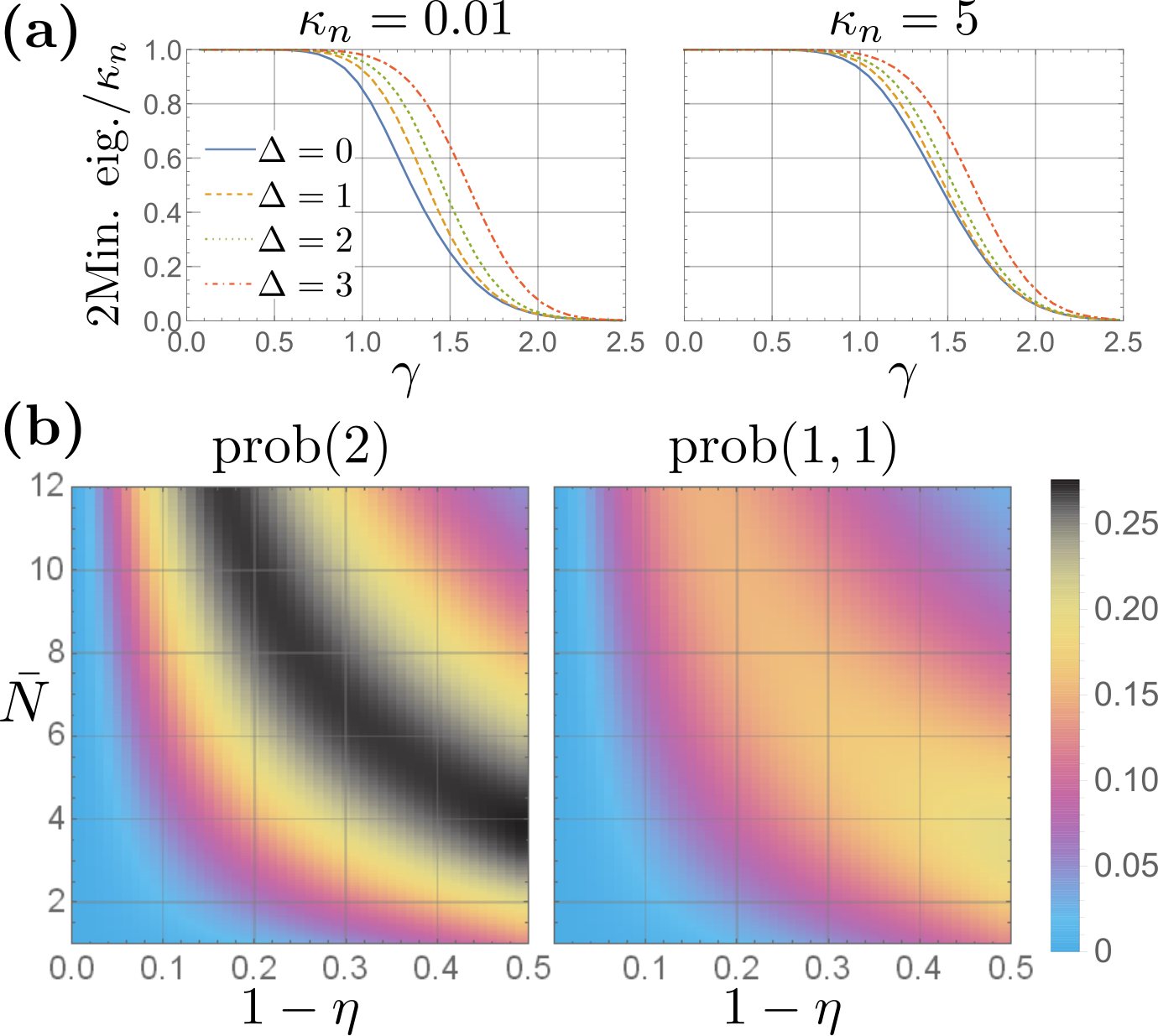
As with the cat codes, it turns out that the dissipator does the job of protecting against dephasing errors for both modes. Since and both commute with , dephasing does not connect code spaces for different values of . (We could have also inferred this much from the above error-correction conditions.) Therefore, we only need to see how dephasing acts within each subspace of fixed . The rates of dephasing-induced logical errors are determined by the eigenvalues of the superoperator , and one can numerically plot those eigenvalues and observe that they are suppressed exponentially as , where is a constant. It is easy to show that the effect of and within a fixed- subspace is identical, so we consider only and plot the dephasing error rates vs. for two values of and four values of in Fig. 1(a).
III.3.2 Loss errors
Now let us turn to loss errors and show that arbitrary instances of and (for ) are correctable. Equations (57a-b) readily tell us that the value of is shifted in different directions upon the respective loss events. Therefore, projecting back onto the original code space yields
| (63) |
The code thus corrects all individual loss errors in both modes. However, the leading uncorrectable error is a simultaneous loss in both modes. Due to the extra bit flip induced by a loss in mode one, induces a bit flip within the code:99 9 If we change the error channel in a way that allows us to know how many total photons were lost (“channel monitoring” [12]), we can track even this error: if the measured but two photons were lost in total, then had to have occurred.
| (64) |
Note that there is no ratio of normalizations this time because the value of is unchanged.
Strictly speaking, the leading uncorrectable cat code error is of the same order as the leading uncorrectable pair-cat code error . So what is the advantage of scheme II over scheme I? While there is no qualitative information-theoretic advantage, the probability of the leading uncorrectable error is slightly lower for scheme II than for scheme I when evaluated for the maximally mixed state for both codes. (We use the maximally mixed state so as to not give preference to any particular superposition of code states. The probabilities below should thus be interpreted as averaged over the code space.) For code I, the probability of losing photons is
| (65) |
where (11) are the Kraus operators for the loss channel. The distribution becomes approximately Poissonian in the large limit [66], but we keep things exact to consider experimentally relevant . Similarly, the probability of loss events in mode and in mode for the maximally mixed code II state is
| (66) |
The leading uncorrectable error probabilities for schemes I and II are thus to , respectively. We plot them in Fig. 1(b) versus the dimensionless loss rate , with transmissivity
| (67) |
and assuming equally lossy cavities (), and the total occupation number,
| (68) |
for scheme I code and scheme II code . One can calculate these analytically, yielding
| (69a) | ||||
| (69b) | ||||
where is the cat normalization factor (25) with and is the pair-cat normalization factor (51b) with . The respective total photon numbers are (for and codes)
| (70) |
Let us compare the uncorrectable error probabilities. At a loss rate and at the optimal (for dephasing) values of the two codes introduced in the previous subsection, we have at the optimal for scheme I and at the optimal for scheme II. While the difference is not large, it shows that the protection from loss of scheme II is no worse than that of scheme I. At and , the difference is more pronounced: for scheme I and for scheme II. A low loss probability allows one to take more time during syndrome measurement, resulting in improved measurement accuracy [32, Supplementary Information Sec. 4.1].
Protection from loss events can be implemented in a continuous manner using additional jump operators
| (71) |
for , provided that and the state is initialized in the codespace [cf. Eq. (30)]. The positive odd case corrects the bit-flip induced by . The alternative cat-code correction scenario from Sec. II.3.2 can also be extended to scheme II by in the bras of Eq. (71). We propose to realize related jumps of the form (131) and , adding photons conditional on a nonzero . These jumps are analogous to those stemming from the continuous QEC proposal of scheme I [53, Sec. 4.2.2].
III.4 Pair-cat code gates
Let us introduce the gates for the setup of scheme II, which are all in complete analogy to those of scheme I.
III.4.1 Hamiltonian and gates
We can once again leverage the fact that is an uncorrectable error and create a gate. Via the same techniques described for the cat codes, the Hamiltonian generates rotations around the -axis:
| (72) |
with corrections exponential in . A two-qubit gate can similarly be created using the Hamiltonian for qubit systems and with respective parameters and :
| (73) |
III.4.2 Hamiltonian -gate
We sketch an extension of the scheme [55] from cat to pair-cat codes. The Josephson junction Hamiltonian now couples to both modes,
| (74) |
where is the Josephson energy, are drive frequencies, and () is the amplitude and phase of the drive of mode one (two). Following Sec. II.4.2, we apply the RWA to the above Hamiltonian, yielding an operator that is diagonal in Fock space, , where is defined in Eq. (34). Once again, since the two basis states (52) we use to represent the code are superpositions of different sets of Fock states, there will be no or terms when under the RWA is projected into the codespace in this basis,
| (75) |
where . Just like the analogous single mode gate is -dependent, this gate is -dependent. However, following Ref. [55], we can in principle combine multiple junctions, each with a Hamiltonian like , but with their own tunable parameters. While making a completely -independent gate is outside the scope of this work, we anticipate that there are sufficient degrees of freedom in such a combination to allow for to be -independent for at least .
III.4.3 Holonomic -gate
Alternatively to the above -gate, we can maintain protection from loss events but suppress protection from dephasing events by adiabatically changing in the sequence . Using the decoherence Hamiltonian and following [67, Sec. IV C], one can verify that the Lindbladian remains gapped throughout the entire adiabatic path. Thus, the leading-order effect is the holonomy induced on the states after the path, which comes from the part . In this step, the new steady states of are , whose limit is . However, the initial states for this step consist of just the Fock states without the extra phase. Thus, to compensate for including the extra phase during the step , one will have . The entire sequence thus performs an effective -rotation
| (76) |
The -dependent phase is an overall phase since the qubit is entirely in a code space of fixed occupation number difference, so the effect of the gate is independent of .
III.4.4 Kerr -rotation
As with cat codes, we can utilize Kerr nonlinearities to form a Hamiltonian and create a -rotation around the -axis of the pair-cat qubit. However, this is less practical than the cat-code gate since it requires coupling several fine-tuned junctions to each mode. Running this evolution for a time yields the operation
| (77) |
This can be proven by substituting the labels for sets of Fock states and for and , respectively, in . Unfortunately, as with cat codes, this does require a relatively large so that no loss events occur during the running of this gate. Alternatively, one can track loss events during the gate by measuring and compensate by applying rotations afterwards.
III.4.5 Kerr control-phase gate
Rounding out Table 1, we can evolve under another combination of Kerr nonlinearities for four modes,
| (78) |
where () is the occupation number difference and () are the occupation number operators for pair-cat qubit 1 (2). Substituting the Fock state components of the two-qubit basis elements into the four occupation number operators yields an effect gate
| (79) |
III.4.6 Control engineering
It turns out that one can use drives and on cavity one and two respectively, an ancilla transmon drive , and the two-cavity dispersive Hamiltonian to implement a universal set of gates for both cavities ([11], Appx. G). Similar schemes have already been implemented experimentally [97], and one could consider using such schemes for pair-cat manipulation. However, as with cat-codes, it is likely that these procedures will have to be performed without the engineered dissipation .

IV Quasiprobability distributions for fixed- subspaces
A generic two-mode state can be represented using two-mode analogues of the -, -, or igner quasiprobability distributions [98]. However, the phase space of the full two-mode system is four-dimensional, so one has to judiciously pick the right two-dimensional cross-sections to study the state. We show here that, if one is restricted to a fixed- sector, a two-dimensional space is sufficient to represent the state. Given pair-coherent states , this space is the complex plane represented by . One should think of this as the fixed- two-mode analogue of the complex plane for a single mode. We suggest not to call this a phase space [99] since the lowest-order physically motivated operators — and — do not commute to a constant; we instead refer to it as the -plane. The derivations below can be repeated for the two fixed-parity subspaces of a single mode using the cat states .
The eigenvalue equation (45) and overcompleteness of (46) are sufficient to define informationally complete analogues of - and -distribution functions in the -plane [100, 101]. Along similar lines and following standard procedures [98], here we also define a generalized -representation. In order to help simplify these distributions, we define
| (80) |
and employ the more conventional set of pair-coherent states
| (81) |
This convention allows us to avoid dealing with whenever we act on these states with . These states also resolve the identity:
| (82) |
where [this measure differs from (47) by the Jacobian ]. Below, we define our distributions (with ) using , but convert back to our convention by examining instead. The reason we do this is because we have found more visually similar to their corresponding single-mode quasiprobability distributions.
Given a state and a fixed occupation number difference , the respective distributions are
| (83a) | ||||
| (83b) | ||||
| (83c) | ||||
where . The three traces are called the characteristic functions of the state, and the distributions are simply their Fourier transforms. These are normalized, , which is easily seen using the identity
| (84) |
Applying Eqs. (81-82) and the above identity to Eq. (83a) yields
| (85) |
This two-mode -distribution provides us with plots that are visually similar to the conventional single-mode -distribution for the various states we have tried (see Fig. 2). Note that, due to the squaring of the argument, all phase space plots are invariant under . This way, pair-coherent states look like cat states (as opposed to coherent states). We argue this is more natural due to the close group-theoretical connection between and .
The -distribution provides a diagonal representation for in terms of ,
| (86) |
We can plug in the above equation into Eq. (83b) and simplify using Eqs. (81-82) to show that is indeed equal to Eq. (83b).
The above distributions can also be used for state tomography, in which the expectation value of an observable is evaluated using only the distribution of the state and the corresponding dual distribution of the observable:
| (87) |
where is a suitable measure. We define to be informationally complete — equivalent to the state itself — if the above equality is satisfied for some . Plugging in Eq. (86) into the left-hand side of Eq. (87) easily yields with . The dual for the characteristic function of the -distribution, , was determined in Ref. [102] (see also [103]). This means that itself is also informationally complete, but it is no longer self-dual as it is in the single-mode case (so it is technically not a proper Wigner distribution [104]). There is currently no analogue of the dramatic simplification that can be done for the conventional Wigner function (see, e.g., [105], Appx. A.2), resulting in time-consuming numerics. We leave its simplification, study, and interpretation to future work, but sketch our code states (52) in Fig. 3 to reveal fringes characteristic of the conventional Wigner distribution.

V Stabilizers & generalizations
We comment on higher-mode generalizations of scheme II, making contact with concepts from stabilizer-based error-correction [106, 62] and its extensions [107, 108, 109, 110, 111, 112, 113].
V.1 Pair-cat code stabilizers
Recall that traditional stabilizer codes, denoted by projection , are defined as unique eigenspaces of eigenvalue one of a set of commuting operators (called stabilizers):
| (88) |
These commuting operators are part of a larger group of operators. We introduce stabilizers for the two-mode case, but by picking stabilizers out of the algebra of two-mode operators instead of a group. In addition, we relax the usual assumptions that are all Hermitian and involutive (square to the identity). While our stabilizers commute, a consequence of this algebraic framework is that some of them are not diagonalizable.
Recall that the logical state set is defined by two parameters: real and integer . The logical subspace is the eigenspace of eigenvalue one of the stabilizers
| (89a) | ||||
| (89b) | ||||
(Similar stabilizers exist for cat codes, and , with the latter an infinite sum of elements of the algebra .) These stabilizers obviously commute and give
| (90) |
when applied to the code subspace projection (54). Since is not Hermitian, (but we do have ) and we cannot straightforwardly construct Hermitian projections out of . The projection constructed out of exponentials of is of course onto a subspace of fixed [see Eq. (41a)]. The stabilizer picks the subspace of fixed occupation number difference while selects the two pair-cat states with the proper value of within that subspace. There are only two pair-coherent states having that value of because of the relations and .
Recall from Sec. III.3 that the code can detect any number of single-mode losses. Consider only operators of the form and let the weight of an operator be the number of modes on which acts nontrivially. Then, we find that detects all weight one errors of this type. However, due to the approximate satisfaction of the diagonal error-correction conditions, this code can exactly correct against such errors only in the limit; for any finite , this is an exact error-detecting and an approximate error-correcting code [114, 115]. The lowest-weight undetectable error is — a sort of square-root of the stabilizer .
V.2 Multimode generalization
The above framework can easily be generalized to multiple modes and qudit codes. Given modes and logical qudit dimension , let
| (91) |
where is the lowering operator for mode . Consider also the occupation number differences
| (92) |
for and a vector of differences
| (93) |
with the corresponding operators . One can then construct eigenstates of all ,
| (94) |
where is the projection on the multimode subspace whose nearest-neighbor occupation value differences are fixed by . The qudit code
| (95) |
can detect any loss errors of weight or less. Superposition of such projected coherent states yields the conjugate “cat” basis,
| (96) |
The form of such “cat” states is especially concise for ,
| (97) |
The lowest-weight undetectable error is . For even , instead of utilizing the entire -dimensional space for each to store information, one can define the two-dimensional subspace as the new logical qubit and use the complementary subspace to protect said qubit from higher-weight errors. (In the single mode case, a more judicious choice of qubit suppresses errors even more [30]; the same is likely true here, but this is outside the scope of this paper.) For example, the generalized states for , obtained by taking (52) and substituting
| (98) |
can detect with . In combination with being able to detect arbitrary single-mode loss events, this means that generalized pair-cat codes can detect up to loss errors in each mode — . The spacing is the same as the spacing discussed in Ref. [30] for “multi-legged” single-mode cat codes and binomial codes. Details as to how pair-cat codes detect are given in Ref. [76].
We have so far considered only photon losses in our error analysis. However, we can equivalently consider two-mode gains and losses and their generalization for multiple modes. In other words, multimode cat codes can protect either against a set of losses or against a different set of losses and gains. For example, the two-mode scheme II can protect against either or or . The latter two sets include only one of the two modes, so this analysis is not particularly useful for . However, higher codes can in fact protect against all single-mode losses and gains. For , a loss (gain) event of photons in mode shifts down (up) by and up (down) by . The edge cases and are handled by positive and negative shifts in and , respectively. Thus, all single-photon losses and gains correspond to a unique syndrome.
V.3 Three-mode example
Consider , , . The range of depends on the values of ,
The three-mode generalized “cat” states (96) — superpositions of the three-mode projected coherent states (94) — have been studied before for this case [116].
The integer differences form the two-dimensional lattice shown in Fig. 4 and each weight-two loss operator shifts to a unique point on the lattice. To prove this, observe that losing one photon in mode 1 [2, 3] shifts you from the origin to the point [, ] on the lattice. Drawing three lines from the origin to these three points and onward to infinity divides the lattice into three regions [Fig. 4(a)], which correspond to the three possible types of at most weight-two operators,
| (99) |
Given a syndrome , one first determines which region it belongs to. Depending on region, the syndrome then corresponds to an error of , , or . The leading undetectable error is .
Alternatively, let us consider protecting against one-photon losses and gains for all three modes,
| (100) |
Considering once more the lattice formed by , events in mode , , or bring about the shifts , , and , respectively, with the sign signaling whether the events were losses or gains. Such errors cover three non-parallel lines in the lattice [Fig. 4(b)], so each error in the above set corresponds to a unique syndrome. Note that in this case, the full lattice of possible syndromes is not utilized; the unused error spaces are colored gray in Fig. 4(b).
V.4 Comparison to other codes
V.4.1 Noon and codes
It is useful to compare this family to the codes [12] and noon codes [10] — two-mode binomial codes [66] concatenated with a repetition code. A fundamental difference is that pair-cat codes consist of infinite superpositions of Fock states while and noon codes are finite-dimensional. In group theory jargon, cat and pair-cat codes live in irreducible subspaces of the non-compact group generated by two-photon loss and occupation number operators (see Sec. III.1), while and noon codes are similarly related to compact groups such as associated with a Hamiltonian [117] and beam-splitter transformations [10], respectively. As a result, only a finite number of photons can be lost for and noon codes while pair-cat codes have a nonzero (albeit exponentially vanishing) probability of losing an arbitrary number of photons. None of the codes correct against more than one individual loss event in each mode, but the two- and three-mode -BC codes can correct more than one loss if one also knows the total number of photons lost.9 Due to concatenation, noon codes require at least four modes to correct single loss events. Generalized two- or higher-mode pair-cat codes with [see Eq. (98)] can detect (and, in the limit, correct) up to loss errors in each mode using only knowledge given from error syndromes. Most importantly, higher-mode pair-cat codes can detect all single-mode losses and gains, something that none of the other codes can do. However, the two mode -BC code can correct dephasing errors exactly up to , while pair-cat codes correct dephasing approximately (see. Sec. III.3). It would be interesting to extend the analysis of Ref. [66] to two modes to determine the theoretically possible performance of these codes against photon loss.
V.4.2 Concatenated cat code
One can consider taking single-mode codes and concatenating with multi-qubit codes. The simplest cat-code cannot correct against photon loss events, so scheme I uses a different set of code states (see Table 1). However, given that all cat-codes suppress dephasing errors for sufficiently large , one can concatenate the simplest cat code with another code that corrects against loss. Loss errors cause a bit-flip within the logical subspace , so concatenating that code with a repetition code yields a code [58] with logical states ()
| (101) |
that can correct both leading-order loss and (for sufficiently large ) dephasing errors in all three modes. This concatenated cat-code (con-cat) is a candidate for a future bosonic logical qubit [53, Sec. 4.3]. Although a full comparison between con-cat and our three-mode code [Eq. (97) for ] is outside the scope of this work, we have reason to believe that pair-cat outperforms con-cat in one-photon-per-mode regime.
Recall that both single- and multi-mode cat codes suppress dephasing errors as and increase, respectively. However, both codes I and II also have the ability to suppress dephasing at optimally configured “sweet spots” , . In Sec. III.3.1, we showed that the two-mode pair-cat code can protect against lowest-order dephasing at the optimal value of photons per mode (). Our three-mode code allows for the same protection at photons per mode (). While the single-mode cat code I also allows for such beneficial fine-tuning, the con-cat code does not because it consists of coherent states whose overlap does not oscillate with increasing . Therefore, con-cat does not have a sweet spot and requires a larger , and thus a larger number of photons, to protect against dephasing.
To corroborate this observation, we calculated a lower bound on the ultimate performance of con-cat and pair-cat, both set at photons. We calculated the entanglement fidelity of both codes, assuming photon loss and the transpose recovery operation. The procedure consists of starting with an initial maximally entangled state of two qubits, encoding one of the qubits in either the con-cat or pair-cat encoding via the isometry , applying the photon loss channel with Kraus operators (11) and equal decay rates to that encoded qubit, recovering via the transpose recovery , and then decoding via the reverse isometry. The entanglement fidelity is the overlap between the state after recovery with the initial state,
| (102) |
where is the identity channel. This is identical to a single-mode code comparison [66, Sec. I.B], with the exception that the recovery used now is not optimal and is fixed to 1.08.1010 10 The three-mode Hilbert space we use has at most photons per mode, yielding dimension . The transpose-recovery calculation took several days on an above-average desktop computer, and calculating the optimal recovery for such a space is intractable. Comparing the transpose recovery fidelity to the optimal one [66, Fig. 1] is unfortunately not fair. However, the transpose recovery is guaranteed to yield a fidelity at most a factor of two from the fidelity of the optimal recovery procedure [118].
The result is shown in Fig. 5; one can see that pair-cat outperforms con-cat for all visible values. In a circuit QED experimental setting, kHz, and we would prefer to correct ten times more often, i.e., at kHz. This yields a , and we observe that pair-cat outperforms con-cat in that regime. While this is only a bound whose infidelity is guaranteed to be within a factor of 1/2 from the optimal result, the improvement of pair-cat over con-cat is more than that, e.g., while at . In fact, pair-cat even reaches a fidelity of 99% at the large loss rate of , which is in the regime of applicability to quantum repeater architectures. This is evidence that pair-cat has a substantial advantage in this low photon regime. However, this does not suggest that pair-cat always outperforms con-cat since increasing for both codes leads to further suppression of dephasing errors in con-cat. Unfortunately, we cannot compare the codes at larger values of because the Hilbert space required to house the states becomes too large to be computationally tractable.
VI Realizing continuous QEC against dephasing
In this section, we propose a realization of a driven-dissipative process corresponding to the left side of Fig. 6 by cascading a pair of two-photon exchange processes using a Raman transition [57]. The sub-system under consideration consists of two high-Q cavity modes coupled to a Josephson junction mode denoted by whose first three states are , , and . The junction mode is in turn coupled to a low-Q resonator for the purpose of entropy extraction. One can engineer an exchange of either of the cavities coupled to the or transitions of the junction mode. Figure 7(a) shows the schematic of cascading two such two-photon exchange processes to get a simultaneous exchange of two photons of each of the cavities with the transition of the junction mode. Subsequent decay of the junction mode translates to the loss of two-photons on both cavities. The reverse process of exciting both cavities simultaneously with two photons each is also possible by exciting the junction mode to the state and then swapping the junction excitation into the cavities.
VI.0.1 Setting up the Hamiltonian
Consider a Hamiltonian consisting of the two high-Q cavities (with lowering operators and frequencies ) and a Josephson junction mode (with lowering operator , frequency , and Josephson energy ) driven by a time-dependent drive . Let
| (103) |
consist of the harmonic portion of the full Hamiltonian. The anharmonic portion of the junction is then , where the phase difference across the junction is
| (104) |
Here, denote the amplitude participation ratios of the respective modes in the junction, with corresponding to the zero point fluctuations of the respective modes as seen by the junction and being the reduced superconducting flux quantum [25]. Combining the harmonic and anharmonic portions with the drive term and assuming that (for all ) and that all mode frequencies are non-commensurate, we expand the cosine to fourth order [25] and obtain our the Hamiltonian
| (105) |
We consider a three-tone drive,
| (106) |
and apply a sequence of transformations which absorbs, one tone at a time, the entire drive into , the anharmonic part of the junction (see Ref. [31], Supplementary Materials). Let us consider tone 1 and go into the rotating frame defined by . The drive term corresponding to tone 1 is now time-independent, so let us displace in order to move that term into . Finally, we move out of the interaction picture using . Due to the displacement, the other two tones produce time-dependent offset terms which are proportional to the identity; we ignore such terms from now on. This procedure is then performed sequentially for tones 2 and 3, yielding
| (107) |
where the new time-dependent phase difference is
| (108) |
and is the displacement of the junction mode due to the th drive.
We now expand the term in order to eventually tune the drives such that our desired terms are selected in a particular rotating frame. Normal-ordering the -term (Lamb- and Stark-)shifts the cavity frequencies to new frequencies (which are here very different from ), so the rotating frame we pick is with respect to the new frequencies. Regarding the junction, we consider only its first three states , defining transition frequencies () between and ( and ). We can absorb the cavity shifts as well as any self-energy terms describing the junction’s first three levels into a noninteracting part
| (109) |
where and are junction states.
Let us consider going into the rotating frame with respect to in order to select the desired terms
| (110) |
in the anharmonic term . The drive () is used to introduce an exchange of two photons of cavity () with the excitation of the junction mode from the () to the () state. The drive frequencies are thus
| (111a) | ||||
| (111b) | ||||
| (111c) | ||||
The frequencies are detuned by [dotted line in Fig. 7(a)] such that together they produce an exchange of two photons in each cavity with the excitation of the junction. The third drive selects the term that, in presence of dissipation, will translate into a simultaneous two-photon drive on both cavities and produce with a nonzero . The rest of the junction levels are ignored under the assumption that the anharmonicity of the junction mode is much greater than the detuning,
| (112) |
A sketch of all this is shown in Fig. 7(b).
Assuming the above approximations and the values of the drive tones, we keep only the diagonal terms and our desired two-photon exchange terms (110) in from Eq. (107). In the rotating frame of , this yields our time-independent system Hamiltonian
| (113) |
where the matrix acts on the junction basis . The remaining piece contains all the non-rotating anharmonic terms of ,
| (114) |
where cavity self- and cross-Kerr terms are and for , respectively. (The difference between comes from the differing strengths of the and transitions.) The new drive strengths are
| (115a) | ||||
| (115b) | ||||
| (115c) | ||||
VI.0.2 Eliminating the junction
Here we show that an effective transition through the detuned state comes at the price of the four photon loss , as desired. This is already hinted in Eq. (113). We first eliminate the state and then, with the help of dissipation, the entire junction. We use second-order perturbation theory for the first part and adiabatic elimination for the second, but note that both parts can also be done either entirely using adiabatic elimination or using a generalization of the RWA [119] (similar to the analogous realization of scheme I [57]). Since the two parts are sequential and not simultaneous, we have to perform the second part — adiabatic elimination — on the timescales during which the perturbation theory is valid.
For the first part, we perform degenerate perturbation theory on the subspace. Let be the unperturbed part of (113), with the remaining parts constituting the perturbation. Letting and adding the first-order () and second-order () corrections to the subspace yields
| (116) |
where is a pseudoinverse and the matrix acts on the subspace. The term gives the expected simultaneous two-photon exchange coupled to the transition of the junction mode.
The second part uses the junction’s intrinsic dissipation, which we assume is of Lindblad form. Within the subspace, we have
| (117) |
We proceed to adiabatically eliminate the -state by the standard procedure {e.g., Ref. [31], Supplementary Materials; see also [120, 121]}. In other words, we turn the Hamiltonian , where here is an operator on the two cavities, into a dissipator with jump operator . We assume the junction is lossy, i.e., is much greater than all of the other parameters in , and derive the effective dynamics of the two cavities under the assumption that the junction is perturbed away from by a small parameter. This yields the two-cavity Lindbladian
| (118) |
with Hamiltonian
| (119) |
and dissipator parameters
| (120) |
VI.0.3 Leading-order error processes
While we have obtained our dissipator above, the Hamiltonian (119) unfortunately carries undesirable anharmonic terms. However, we have the ability to cancel the anharmonicity of the mode by adjusting the parameters to achieve . Note that the anharmonicity of the mode remains unchanged.
The above procedure eliminating the junction unfortunately carries with it one more leading-order error, which we have omitted previously for simplicity. Physically, this corresponds to the ability of the junction state to decay from back to instead of following through the virtual transition to [see Fig. 7(a)]. After elimination of , this induces a two-photon loss in the -mode. This process was not accounted for in our previous derivations because we had not introduced dissipation until after we eliminated . If we include the dissipation and perform adiabatic elimination of , we find that (118) gains the term
| (121) |
However, this two-photon dissipation can be corrected if we engineer a device that can measure at least five distinct values of (see Fig. 8 and the next Subsection). This is a key difference between the analogous experimental realization of scheme I [57] and the design here. While the analogous leading-order dissipative error leads to uncorrectable logical errors for cat codes, here such an error can in principle be corrected.
In terms of the additional -mode anharmonicity in (119) and the inherited -mode two-photon dissipation (121), the and modes are not on equal footing. This asymmetry has been built into the dynamics owing to the fact that couples to the transition and couples to the transition of the junction mode. However, by carefully canceling one of the anharmonicities and discrete error-correction, we have shown that the undesirable effect of this asymmetry can be minimized.
VII Realizing discrete QEC against photon loss

In this section, we propose a way to realize discrete QEC against photon loss. The proposal involves using the four-wave mixing capabilities of two Josephson junction modes to link the displacement of a low-Q resonator mode to the photon number difference between the two high-Q modes.
As shown in Fig. 8, we have two junction modes coupling the two cavities to a low-Q readout cavity . It is assumed that cavity couples only to junction and cavity couples only to junction . Both junctions couple to cavity . It is assumed that the two junction modes are isolated from each other and can be driven independently. The two junctions and cavity are driven with drives parameterized by , respectively. Assuming and expanding the anharmonic parts of the two junctions yields
| (122) | ||||
where is the harmonic part, the phase differences across the junctions are
| (123a) | ||||
| (123b) | ||||
and are the amplitude participation ratios. The two junctions are both independently driven at the frequency of the low-Q cavity, which we set to be the shifted frequency of mode after normal ordering. We also apply a direct resonant drive on the low-Q cavity of strength ; the importance of this drive will be clear in the next couple of steps.
We absorb the -drives on the junction modes in the respective anharmonicities [similar to Eq. (107)], but leave the -cavity drive untouched. This yields
| (124) | ||||
where the time-dependent phase differences are
| (125a) | ||||
| (125b) | ||||
and are the displacements of the junction modes due to the respective drives. Finally, we normal-order the anharmonicities, go into a rotating frame with respect to the Lamb- and Stark-shifted shifted harmonic part,
| (126) |
and keep only the non-rotating terms. Since the only drive frequency is , the only off-diagonal time-independent terms are those for which the number of terms is equal to the number of terms plus the number of terms (and their Hermitian conjugates). We also assume that the junction modes are never resonantly driven and hence are never populated. Therefore, for the sake of compactness, we drop all the diagonal terms involving the operator. The system Hamiltonian becomes
| (127) |
where the couplings are
| (128a) | ||||
| (128b) | ||||
| (128c) | ||||
| (128d) | ||||
| (128e) | ||||
The remaining step now is to tune the second line of Eq. (127) such that we obtain the term . We can adjust the amplitude and the phase of such that
| (129) |
For , , , and , the magnitude of the terms in Eqs. (128a) and (128e) becomes minimal. The remaining can be canceled by setting , yielding
| (130) |
Hence we can engineer the displacement term of the low-Q cavity mode to be proportional to the error syndrome measurement operator (5).
In an idealized scenario (with the -, -, and -dependent terms ignored) and in presence of dissipation with rate , the steady state of the low-Q cavity is a coherent state , where is the complex amplitude of the coherent state. We sketch a simplified IQ phase diagram in Fig. 8, showing this state for different values of . If , the average photon number occupation of the steady state is given by . This should enable us to perform single-shot measurements of the error syndrome using typical heterodyne detection of the signal coming out of the low-Q cavity by employing a quantum limited amplifier, e.g., the Josephson Parametric Converter [122]. After measurement, we can continue tracking the shifts (in the spirit of Pauli frames) and take it into account when decoding.
We conclude by commenting on the -, -, and -dependent terms in Eq. (130). Such terms will necessarily distort the idealized signal, as the full linear part of the cavity Hamiltonian corresponds to an oscillator displaced by and squeezed by and there are several nonlinearities in the system. While these corrections will make the states corresponding to different values of harder to resolve, it will nevertheless be possible since the states manifestly occupy different portions of phase space. We thus leave further optimization of this scheme to future work.

VIII Realizing continuous QEC against photon loss
In this section, we propose a way to continuously correct against photon loss. Since we only need one form of QEC against loss, this proposal is meant to substitute the discrete QEC proposal of the previous section. Instead of coupling the cavities storing the pair-cat qubit to an ancillary cavity, we couple them to an ancillary junction mode through two three-wave mixers dubbed Superconducting Nonlinear Asymmetric Inductive eLements (SNAILs) [56]. Schematically, we substitute the circuit to the right of the two cavities in Fig. 6(a) with the circuit in Fig. 9(a). The main idea is to compensate single photon losses in either cavity by adding photon gain jump operators that are conditional on . For mode , the jump operator is
| (131) |
and similarly for mode . A difference between these jumps and the ideal continuous QEC jumps (71) with is the extra raising operator. Even though this recovery implements first-order dephasing errors or when combined with the preceding loss event, these have negligible effect on the code states for sufficiently large (see Subsec. III.3). We now sketch this proposal, focusing on correction for (mode loss) only [sketched in Fig. 6(b)]. Note that this proposal is similar in spirit to a continuous QEC proposal for scheme I [53, Sec. 4.2.2] and is extendable to higher in natural fashion [see Fig. 9(b)]. In the exposition below, we apply perturbation theory sequentially. However, all terms can be introduced simultaneously in a more involved calculation that yields the same low-order result with higher order corrections.
The SNAIL three-wave mixer provides Jaynes-Cummings type couplings between the junction and the cavities without any additional Kerr nonlinearities. We thus begin with a two-mode driven Jaynes-Cummings Hamiltonian
| (132) | ||||
with cavity frequencies , Josephson junction frequency , real pump drive , and pump frequencies . Setting and and going into the rotating frame with respect to for . The pump strengths are then set so we are in the dispersive regime: with being the average occupation number in cavity [123, Sec. 19.3]. In the dispersive limit, the Hamiltonian becomes . This -dependent junction frequency is responsible for the telescope of levels in Fig. 9(b). For each pair of levels, the two cavities are in the subspace of fixed while the junction is either in for the bottom level or in for the top. Note that we can use this Hamiltonian to perform error syndrome readout, but this scheme is slower than the one from Sec. VII since the readout here would have to be performed bit by bit. Instead of utilizing this for discrete readout, we now describe how to continuously perform the correction operation.
Since the junction frequency depends on the error syndrome, we can add photons to the cavity selectively depending on . In particular, for , we utilize the SNAILs to couple the junction to cavity via the (counter-rotating) term with frequency in the rotating frame with respect to . We set , the frequency of the effective two-level system at from Fig. 9(b). The Hamiltonian is then
| (133) |
with . Going into the rotating frame with respect to yields the desired transition
| (134) |
Furthermore, assuming the junction decays with jump operator and adiabatically eliminating the junction yields a dissipator with jump operator (131). Thus, we have our desired result to first-order in the RWA.
IX Conclusion
In a non-trivial extension of cat-codes to multiple modes, we introduce a family of two-mode continuous-variable codes based on pair-coherent states (also known as Barut-Girardello states). We analyze which errors the code can correct and extend single-mode cat-code gates to this paradigm. We provide several experimental realizations of the full error-correction scheme associated with this code, including continuous error-correction based on reservoir engineering and discrete (i.e., measurement-based) error-correction based on measurements of the occupation number difference between the two modes. We introduce ways to completely visualize certain two-mode states in a two-dimensional complex plane, avoiding the need to take cross-sections of the states’ four-dimensional Wigner functions. An extension of the codes to multiple modes makes contact with the stabilizer formalism from multi-qubit error correction and yields codes which can simultaneously correct against single-mode losses and gains.
Acknowledgements.
The authors thank Mazyar Mirrahimi and Kyungjoo Noh for fruitful discussions. We acknowledge support from the ARL-CDQI, ARO (Grants No. W911NF-14-1-0011 and No. W911NF-14-1-0563), ARO MURI (W911NF-16-1-0349), NSF (EFMA-1640959), AFOSR MURI (FA9550-14-1-0052 and No. FA9550-15-1-0015), the Alfred P. Sloan Foundation (BR2013-049), the Packard Foundation (2013-39273), and the Walter Burke Institute for Theoretical Physics at Caltech.References
- [1] S. L. Braunstein and P. van Loock, Quantum information with continuous variables, Rev. Mod. Phys. 77 (2005).
- [2] C. Weedbrook, S. Pirandola, R. García-Patrón, N. J. Cerf, T. C. Ralph, J. H. Shapiro, and S. Lloyd, Gaussian quantum information, Rev. Mod. Phys. 84, 621 (2012).
- [3] N. J. Cerf, G. Leuchs, and E. S. Polzik, Quantum Information with Continuous Variables of Atoms and Light (World Scientific, London, 2007).
- [4] A. Serafini, Quantum Continuous Variables: A Primer of Theoretical Methods (CRC Press, Boca Raton FL, 2017).
- [5] I. L. Chuang and Y. Yamamoto, Simple quantum computer, Phys. Rev. A 52, 3489 (1995).
- [6] I. L. Chuang, D. W. Leung, and Y. Yamamoto, Bosonic quantum codes for amplitude damping, Phys. Rev. A 56, 1114 (1997).
- [7] E. Knill, R. Laflamme, and G. J. Milburn, A scheme for efficient quantum computation with linear optics, Nature 409, 46 (2001).
- [8] T. C. Ralph, A. J. F. Hayes, and A. Gilchrist, Loss-Tolerant Optical Qubits, Phys. Rev. Lett. 95, 100501 (2005).
- [9] W. Wasilewski and K. Banaszek, Protecting an optical qubit against photon loss, Phys. Rev. A 75, 042316 (2007).
- [10] M. Bergmann and P. van Loock, Quantum error correction against photon loss using NOON states, Phys. Rev. A 94, 012311 (2016a).
- [11] M. H. Michael, M. Silveri, R. T. Brierley, V. V. Albert, J. Salmilehto, L. Jiang, and S. M. Girvin, New Class of Quantum Error-Correcting Codes for a Bosonic Mode, Phys. Rev. X 6, 031006 (2016).
- [12] M. Y. Niu, I. L. Chuang, and J. H. Shapiro, Hardware-efficient bosonic quantum error-correcting codes based on symmetry operators, Phys. Rev. A 97, 032323 (2018a).
- [13] S. Lloyd and J.-J. E. Slotine, Analog Quantum Error Correction, Phys. Rev. Lett. 80, 4088 (1998).
- [14] S. L. Braunstein, Error Correction for Continuous Quantum Variables, Phys. Rev. Lett. 80, 4084 (1998).
- [15] D. Gottesman, A. Yu. Kitaev, and J. Preskill, Encoding a qubit in an oscillator, Phys. Rev. A 64, 012310 (2001).
- [16] N. C. Menicucci, Fault-Tolerant Measurement-Based Quantum Computing with Continuous-Variable Cluster States, Phys. Rev. Lett. 112, 120504 (2014).
- [17] P. Hayden, S. Nezami, G. Salton, and B. C. Sanders, Spacetime replication of continuous variable quantum information, New J. Phys. 18, 083043 (2016).
- [18] A. Ketterer, A. Keller, S. P. Walborn, T. Coudreau, and P. Milman, Quantum information processing in phase space: A modular variables approach, Phys. Rev. A 94, 022325 (2016).
- [19] P. T. Cochrane, G. J. Milburn, and W. J. Munro, Macroscopically distinct quantum-superposition states as a bosonic code for amplitude damping, Phys. Rev. A 59, 2631 (1999).
- [20] J. Niset, U. L. Andersen, and N. J. Cerf, Experimentally Feasible Quantum Erasure-Correcting Code for Continuous Variables, Phys. Rev. Lett. 101, 130503 (2008).
- [21] Z. Leghtas, G. Kirchmair, B. Vlastakis, R. J. Schoelkopf, M. H. Devoret, and M. Mirrahimi, Hardware-Efficient Autonomous Quantum Memory Protection, Phys. Rev. Lett. 111, 120501 (2013).
- [22] F. Lacerda, J. M. Renes, and V. B. Scholz, Coherent state constellations for Bosonic Gaussian channels, 2016 IEEE Int. Symp. Inf. Theory , 2499 (2016).
- [23] S.-W. Lee and H. Jeong, Near-deterministic quantum teleportation and resource-efficient quantum computation using linear optics and hybrid qubits, Phys. Rev. A 87, 022326 (2013).
- [24] E. Kapit, Hardware-Efficient and Fully Autonomous Quantum Error Correction in Superconducting Circuits, Phys. Rev. Lett. 116, 150501 (2016).
- [25] S. M. Girvin, in Quantum Mach. Meas. Control Eng. quantum Syst., edited by M. H. Devoret, B. Huard, R. J. Schoelkopf, and L. F. Cugliandolo (Oxford University Press, Oxford, 2015) Chap. 3.
- [26] X. Gu, A. F. Kockum, A. Miranowicz, Y.-x. Liu, and F. Nori, Microwave photonics with superconducting quantum circuits, Phys. Rep. 718-719, 1 (2017).
- [27] M. Mirrahimi, Z. Leghtas, V. V. Albert, S. Touzard, R. J. Schoelkopf, L. Jiang, and M. H. Devoret, Dynamically protected cat-qubits: a new paradigm for universal quantum computation, New J. Phys. 16, 045014 (2014).
- [28] V. V. Albert, C. Shu, S. Krastanov, C. Shen, R.-B. Liu, Z.-B. Yang, R. J. Schoelkopf, M. Mirrahimi, M. H. Devoret, and L. Jiang, Holonomic Quantum Control with Continuous Variable Systems, Phys. Rev. Lett. 116, 140502 (2016a).
- [29] M. Bergmann and P. van Loock, Quantum error correction against photon loss using multicomponent cat states, Phys. Rev. A 94, 042332 (2016b).
- [30] L. Li, C.-l. Zou, V. V. Albert, S. Muralidharan, S. M. Girvin, and L. Jiang, Cat Codes with Optimal Decoherence Suppression for a Lossy Bosonic Channel, Phys. Rev. Lett. 119, 030502 (2017).
- [31] Z. Leghtas, S. Touzard, I. M. Pop, A. Kou, B. Vlastakis, A. Petrenko, K. M. Sliwa, A. Narla, S. Shankar, M. J. Hatridge, M. Reagor, L. Frunzio, R. J. Schoelkopf, M. Mirrahimi, and M. H. Devoret, Confining the state of light to a quantum manifold by engineered two-photon loss, Science (80-. ). 347, 853 (2015).
- [32] N. Ofek, A. Petrenko, R. Heeres, P. Reinhold, Z. Leghtas, B. Vlastakis, Y. Liu, L. Frunzio, S. M. Girvin, L. Jiang, M. Mirrahimi, M. H. Devoret, and R. J. Schoelkopf, Extending the lifetime of a quantum bit with error correction in superconducting circuits, Nature 536, 441 (2016).
- [33] R. W. Heeres, P. Reinhold, N. Ofek, L. Frunzio, L. Jiang, M. H. Devoret, and R. J. Schoelkopf, Implementing a universal gate set on a logical qubit encoded in an oscillator, Nat. Commun. 8, 94 (2017).
- [34] P. Arrangoiz-Arriola, E. A. Wollack, M. Pechal, J. D. Witmer, J. T. Hill, and A. H. Safavi-Naeini, Coupling a Superconducting Quantum Circuit to a Phononic Crystal Defect Cavity, Phys. Rev. X 8, 031007 (2018).
- [35] Y. Chu, P. Kharel, W. H. Renninger, L. D. Burkhart, L. Frunzio, P. T. Rakich, and R. J. Schoelkopf, Quantum acoustics with superconducting qubits, Science (80-. ). 358, 199 (2017).
- [36] J. F. Poyatos, J. I. Cirac, and P. Zoller, Quantum Reservoir Engineering with Laser Cooled Trapped Ions, Phys. Rev. Lett. 77, 4728 (1996).
- [37] A. A. Belavin, B. Ya. Zel’dovich, A. M. Perelomov, and V. S. Popov, Relaxation of Quantum Systems with Equidistant Spectra, Sov. Phys. JETP-USSR 29, 145 (1969).
- [38] G. Lindblad, On the generators of quantum dynamical semigroups, Commun. Math. Phys. 48, 119 (1976).
- [39] V. Gorini, A. Kossakowski, and E. C. G. Sudarshan, Completely positive dynamical semigroups of N-level systems, J. Math. Phys. 17, 821 (1976).
- [40] L.-M. Duan and G.-C. Guo, Preserving Coherence in Quantum Computation by Pairing Quantum Bits, Phys. Rev. Lett. 79, 1953 (1997).
- [41] P. Zanardi and M. Rasetti, Noiseless Quantum Codes, Phys. Rev. Lett. 79, 3306 (1997).
- [42] D. A. Lidar, I. L. Chuang, and K. B. Whaley, Decoherence-Free Subspaces for Quantum Computation, Phys. Rev. Lett. 81, 2594 (1998).
- [43] B. M. Terhal, Quantum error correction for quantum memories, Rev. Mod. Phys. 87, 307 (2015).
- [44] J. P. Paz and W. H. Zurek, Continuous error correction, Proc. R. Soc. A 454 (1998).
- [45] J. P. Barnes and W. S. Warren, Automatic Quantum Error Correction, Phys. Rev. Lett. 85, 856 (2000).
- [46] C. Ahn, A. C. Doherty, and A. J. Landahl, Continuous quantum error correction via quantum feedback control, Phys. Rev. A 65, 042301 (2002).
- [47] M. Sarovar and G. J. Milburn, Continuous quantum error correction by cooling, Phys. Rev. A 72, 012306 (2005).
- [48] O. Oreshkov and T. A. Brun, Continuous quantum error correction for non-Markovian decoherence, Phys. Rev. A 76, 022318 (2007).
- [49] J. Kerckhoff, H. I. Nurdin, D. S. Pavlichin, and H. Mabuchi, Designing Quantum Memories with Embedded Control: Photonic Circuits for Autonomous Quantum Error Correction, Phys. Rev. Lett. 105, 040502 (2010).
- [50] J. Kerckhoff, D. S. Pavlichin, H. Chalabi, and H. Mabuchi, Design of nanophotonic circuits for autonomous subsystem quantum error correction, New J. Phys. 13, 055022 (2011).
- [51] G. Sarma and H. Mabuchi, Gauge subsystems, separability and robustness in autonomous quantum memories, New J. Phys. 15, 035014 (2013).
- [52] J.-M. Lihm, K. Noh, and U. R. Fischer, Implementation-independent sufficient condition of the Knill-Laflamme type for the autonomous protection of logical qudits by strong engineered dissipation, Phys. Rev. A 98, 012317 (2018).
- [53] J. Cohen, Autonomous quantum error correction with superconducting qubits, Ph.D. thesis, Ecole Normale Superieure (2017).
- [54] L. Sun, A. Petrenko, Z. Leghtas, B. Vlastakis, G. Kirchmair, K. M. Sliwa, A. Narla, M. Hatridge, S. Shankar, J. Blumoff, L. Frunzio, M. Mirrahimi, M. H. Devoret, and R. J. Schoelkopf, Tracking photon jumps with repeated quantum non-demolition parity measurements. Nature 511, 444 (2014).
- [55] J. Cohen, W. C. Smith, M. H. Devoret, and M. Mirrahimi, Degeneracy-Preserving Quantum Nondemolition Measurement of Parity-Type Observables for Cat Qubits, Phys. Rev. Lett. 119, 060503 (2017).
- [56] N. E. Frattini, U. Vool, S. Shankar, A. Narla, K. M. Sliwa, and M. H. Devoret, 3-wave mixing Josephson dipole element, Appl. Phys. Lett. 110, 222603 (2017).
- [57] S. O. Mundadha, A. Grimm, S. Touzard, U. Vool, S. Shankar, M. H. Devoret, and M. Mirrahimi, Generating higher-order quantum dissipation from lower-order parametric processes, Quantum Sci. Technol. 2, 24005 (2017).
- [58] W. J. Munro, K. Nemoto, G. J. Milburn, and S. L. Braunstein, Weak-force detection with superposed coherent states, Phys. Rev. A 66, 023819 (2002).
- [59] Y. Zhang, X. Zhao, Z.-F. Zheng, L. Yu, Q.-P. Su, and C.-P. Yang, Universal controlled-phase gate with cat-state qubits in circuit QED, Phys. Rev. A 96, 052317 (2017).
- [60] C. H. Bennett, D. P. DiVincenzo, J. A. Smolin, and W. K. Wootters, Mixed-state entanglement and quantum error correction, Phys. Rev. A 54, 3824 (1996).
- [61] E. Knill and R. Laflamme, Theory of quantum error-correcting codes, Phys. Rev. A 55, 900 (1997).
- [62] M. A. Nielsen and I. L. Chuang, Quantum Computation and Quantum Information (Cambridge University Press, Cambridge, 2011).
- [63] M. Ueda, Probability-density-functional description of quantum photodetection processes, Quantum Opt. 1, 131 (1989).
- [64] C. T. Lee, Superoperators and their implications in the hybrid model for photodetection, Phys. Rev. A 49, 4888 (1994).
- [65] A. B. Klimov and S. M. Chumakov, A Group-Theoretical Approach to Quantum Optics (Wiley, Weinheim, 2009).
- [66] V. V. Albert, K. Noh, K. Duivenvoorden, D. J. Young, R. T. Brierley, P. Reinhold, C. Vuillot, L. Li, C. Shen, S. M. Girvin, B. M. Terhal, and L. Jiang, Performance and structure of single-mode bosonic codes, Phys. Rev. A 97, 032346 (2018).
- [67] V. V. Albert, B. Bradlyn, M. Fraas, and L. Jiang, Geometry and Response of Lindbladians, Phys. Rev. X 6, 041031 (2016b).
- [68] P. Zanardi and L. Campos Venuti, Coherent Quantum Dynamics in Steady-State Manifolds of Strongly Dissipative Systems, Phys. Rev. Lett. 113, 240406 (2014).
- [69] R. Azouit, A. Sarlette, and P. Rouchon, in 2016 IEEE 55th Conf. Decis. Control (IEEE, 2016) pp. 4559–4565.
- [70] P. Facchi and S. Pascazio, Quantum Zeno Subspaces, Phys. Rev. Lett. 89, 080401 (2002).
- [71] C. Arenz, D. Burgarth, P. Facchi, V. Giovannetti, H. Nakazato, S. Pascazio, and K. Yuasa, Universal Control Induced by Noise, Phys. Rev. A 93, 062308 (2016).
- [72] B. Buča and T. Prosen, A note on symmetry reductions of the Lindblad equation: transport in constrained open spin chains, New J. Phys. 14, 073007 (2012).
- [73] V. V. Albert and L. Jiang, Symmetries and conserved quantities in Lindblad master equations, Phys. Rev. A 89, 022118 (2014).
- [74] V. V. Dodonov, I. Malkin, and V. Man’ko, Even and odd coherent states and excitations of a singular oscillator, Physica 72, 597 (1974).
- [75] M. T. Vaughn, Introduction to Mathematical Physics (Wiley, Weinheim, 2007).
- [76] V. V. Albert, Lindbladians with multiple steady states: theory and applications, Ph.D. thesis, Yale University (2017).
- [77] S. Puri, S. Boutin, and A. Blais, Engineering the quantum states of light in a Kerr-nonlinear resonator by two-photon driving, npj Quantum Inf. 3, 18 (2017).
- [78] M. Ippoliti, L. Mazza, M. Rizzi, and V. Giovannetti, Perturbative approach to continuous-time quantum error correction, Phys. Rev. A 91, 042322 (2015).
- [79] F. Reiter, A. S. Sørensen, P. Zoller, and C. A. Muschik, Dissipative quantum error correction and application to quantum sensing with trapped ions, Nat. Commun. 8, 1822 (2017).
- [80] J. Cohen and M. Mirrahimi, Dissipation-induced continuous quantum error correction for superconducting circuits, Phys. Rev. A 90, 062344 (2014).
- [81] E. Knill, Quantum computing with realistically noisy devices, Nature 434, 39 (2005).
- [82] F. Wilczek and A. Zee, Appearance of Gauge Structure in Simple Dynamical Systems, Phys. Rev. Lett. 52, 2111 (1984).
- [83] S. Krastanov, V. V. Albert, C. Shen, C.-L. Zou, R. Heeres, B. Vlastakis, R. Schoelkopf, and L. Jiang, Universal control of an oscillator with dispersive coupling to a qubit, Phys. Rev. A 92, 040303(R) (2015).
- [84] R. W. Heeres, B. Vlastakis, E. Holland, S. Krastanov, V. V. Albert, L. Frunzio, L. Jiang, and R. J. Schoelkopf, Cavity State Manipulation Using Photon-Number Selective Phase Gates, Phys. Rev. Lett. 115, 137002 (2015).
- [85] C. Shen, K. Noh, V. V. Albert, S. Krastanov, M. H. Devoret, R. J. Schoelkopf, S. M. Girvin, and L. Jiang, Quantum channel construction with circuit quantum electrodynamics, Phys. Rev. B 95, 134501 (2017).
- [86] S. Lloyd and L. Viola, Engineering quantum dynamics, Phys. Rev. A 65, 010101 (2001).
- [87] E. Andersson and D. K. L. Oi, Binary search trees for generalized measurements, Phys. Rev. A 77, 052104 (2008).
- [88] R. Iten, R. Colbeck, and M. Christandl, Quantum circuits for quantum channels, Phys. Rev. A 95, 052316 (2017).
- [89] A. O. Barut and L. Girardello, New “coherent” states associated with non-compact groups, Commun. Math. Phys. 21, 41 (1971).
- [90] G. S. Agarwal, Generation of Pair Coherent States and Squeezing via the Competition of Four-Wave Mixing and Amplified Spontaneous Emission, Phys. Rev. Lett. 57, 827 (1986).
- [91] G. S. Agarwal, Nonclassical statistics of fields in pair coherent states, J. Opt. Soc. Am. B 5, 1940 (1988).
- [92] A. M. Perelomov, Generalized Coherent States and Their Applications (Springer, Berlin, 1986).
- [93] C. C. Gerry and R. Grobe, Nonclassical properties of correlated two-mode Schrodinger cat states, Phys. Rev. A 51, 1698 (1995).
- [94] S.-C. Gou, J. Steinbach, and P. L. Knight, Vibrational pair cat states, Phys. Rev. A 54, 4315 (1996).
- [95] X.-M. Liu, Even and odd charge coherent states and their non-classical properties, Phys. Lett. A 279, 123 (2001).
- [96] J. R. Choi and K. H. Yeon, SU(1,1) Coherent States for the Generalized Two-Mode Time-Dependent Quadratic Hamiltonian System, Int. J. Theor. Phys. 47, 1891 (2008).
- [97] C. Wang, Y. Y. Gao, P. Reinhold, R. W. Heeres, N. Ofek, K. Chou, C. Axline, M. Reagor, J. Blumoff, K. M. Sliwa, L. Frunzio, S. M. Girvin, L. Jiang, M. Mirrahimi, M. H. Devoret, and R. J. Schoelkopf, A Schrodinger cat living in two boxes, Science (80-. ). 352, 1087 (2016).
- [98] M. Hillery, R. O’Connell, M. Scully, and E. Wigner, Distribution functions in physics: Fundamentals, Phys. Rep. 106, 121 (1984).
- [99] R. F. Werner, Uncertainty relations for general phase spaces, Front. Phys. 11, 110305 (2016).
- [100] C. Brif and Y. Ben-Aryeh, Subcoherent p-representation for non-classical photon states, Quantum Opt. 6, 391 (1994).
- [101] D. Popov, Barut-Girardello coherent states of the pseudoharmonic oscillator, J. Phys. A Math. Gen. 34, 5283 (2001).
- [102] G. M. D’Ariano, E. De Vito, and L. Maccone, SU(1,1) tomography, Phys. Rev. A 64, 033805 (2001).
- [103] C. Carmeli, G. Cassinelli, and F. Zizzi, Generalized Orthogonality Relations and SU(1,1)-Quantum Tomography, Found. Phys. 39, 521 (2009).
- [104] C. Ferrie, Quasi-probability representations of quantum theory with applications to quantum information science, Rep. Prog. Phys. 74, 116001 (2011).
- [105] S. Haroche and J.-M. Raimond, Exploring the quantum: atoms, cavities, and photons (Oxford University Press, Oxford, 2006).
- [106] D. Gottesman, Stabilizer codes and quantum error correction, Ph.D. thesis, California Institute of Technology (1997).
- [107] E. Knill, Group Representations, Error Bases and Quantum Codes, (1996), arXiv:9608049 [quant-ph] .
- [108] H. Pollatsek and M. B. Ruskai, Permutationally invariant codes for quantum error correction, Linear Algebr. Appl. 392, 255 (2004).
- [109] S. Y. Looi, L. Yu, V. Gheorghiu, and R. B. Griffiths, Quantum-error-correcting codes using qudit graph states, Phys. Rev. A 78, 042303 (2008).
- [110] A. Cross, G. Smith, J. A. Smolin, and B. Zeng, Codeword Stabilized Quantum Codes, IEEE Trans. Inf. Theory 55, 433 (2009).
- [111] C. Kruszynska and B. Kraus, Local entanglability and multipartite entanglement, Phys. Rev. A 79, 052304 (2009).
- [112] M. Rossi, M. Huber, D. Bruß, and C. Macchiavello, Quantum hypergraph states, New J. Phys. 15, 113022 (2013).
- [113] X. Ni, O. Buerschaper, and M. Van den Nest, A non-commuting stabilizer formalism, J. Math. Phys. 56, 052201 (2015).
- [114] D. W. Leung, M. A. Nielsen, I. L. Chuang, and Y. Yamamoto, Approximate quantum error correction can lead to better codes, Phys. Rev. A 56, 2567 (1997).
- [115] C. Crépeau, D. Gottesman, and A. Smith, in Adv. Cryptol. - EUROCRYPT 2005. Lect. Notes Comput. Sci. vol. 3494, edited by R. Cramer (Springer, Berlin, Heidelberg, 2005) pp. 285–301.
- [116] N. B. An, Even and odd trio coherent states: number distribution, squeezing and realization scheme, Phys. Lett. A 312, 268 (2003).
- [117] M. Y. Niu, I. L. Chuang, and J. H. Shapiro, Qudit-Basis Universal Quantum Computation Using chi-squared Interactions, Phys. Rev. Lett. 120, 160502 (2018b).
- [118] H. K. Ng and P. Mandayam, Simple approach to approximate quantum error correction based on the transpose channel, Phys. Rev. A 81, 062342 (2010).
- [119] M. Mirrahimi and P. Rouchon, Modeling and Control of Quantum Systems, (2015).
- [120] H. J. Carmichael, Statistical Methods in Quantum Optics 2: Non-classical fields (Springer-Verlag, Berlin/Heidelberg, 2008).
- [121] F. Verstraete, M. M. Wolf, and J. I. Cirac, Quantum computation and quantum-state engineering driven by dissipation, Nat. Phys. 5, 633 (2009).
- [122] M. Hatridge, S. Shankar, M. Mirrahimi, F. Schackert, K. Geerlings, T. Brecht, K. M. Sliwa, B. Abdo, L. Frunzio, S. M. Girvin, R. J. Schoelkopf, and M. H. Devoret, Quantum Back-Action of an Individual Variable-Strength Measurement, Science (80-. ). 339, 178 (2013).
- [123] M. O. Scully and M. S. Zubairy, Quantum Optics (Cambridge University Press, Cambridge, 1997).