跳到论文正文
W Papers独立论文阅读器 arXiv:1801.05794 论文正文 计算阅读时间 · 0%
引用这篇论文根据当前论文元数据生成,正式投稿前建议核对。


License: arXiv.org perpetual non-exclusive license
arXiv:1801.05794v2 [math.NA] 30 Apr 2019
\setbibdata

1xx462017 AN UNCONDITIONALLY STABLE SEMI-IMPLICIT CUTFEM

An unconditionally stable semi-implicit CutFEM for an interaction problem between an elastic membrane and an incompressible fluidThanks: Received… Accepted… Published online on… Recommended by…. This research was supported by the National Science Foundation Division of Mathematical Sciences Grant No. 1522663 Higher-Order Methods for Interface Problems with Non-Aligned Meshes.

Kyle Dunn22 2 Now at Cold Regions Research and Engineering Laboratory - U.S. Army ERDC, Hanover, NH 03755, (Kyle.G.Dunn@usace.army.mil) 33 3 Mathematical Sciences Department, Worcester Polytechnic Institute, Worcester, MA 01609, ({rlui, msarkis}@wpi.edu)    Roger Lui 33 3 Mathematical Sciences Department, Worcester Polytechnic Institute, Worcester, MA 01609, ({rlui, msarkis}@wpi.edu)    Marcus Sarkis55footnotemark: 5
Abstract

In this paper we introduce a finite element method for the Stokes equations with a massless immersed membrane. This membrane applies normal and tangential forces affecting the velocity and pressure of the fluid. Additionally, the points representing this membrane move with the local fluid velocity. We design and implement a high-accuracy cut finite element method (CutFEM) which enables the use of a structured mesh that is not aligned with the immersed membrane and then we formulate a time discretization that yields an unconditionally energy stable scheme. We prove that the stability is not restricted by the parameter choices that constrained previous finite element immersed boundary methods and illustrate the theoretical results with numerical simulations.

keywords
immersed boundary method, finite element method, numerical stability, CutFEM, unfitted methods
{AMS}

65N12, 65N30, 74F10

1 Introduction

Fluid dynamics problems with immersed boundaries have arisen in many real world scenarios such as cardiac blood flow [38, 40] and cell mechanics [2]. Two prevalent ideas are the immersed boundary method introduced by Peskin [39] and the immersed interface method by LeVeque and Li [29, 30]. These are both finite difference methods developed for very involved problems. We note that the immersed interface method was also extended to the finite element method by imposing flux conservation and continuity of the solution strongly at certain points of Γ\Gamma; see [1, 11, 15, 16, 19, 20, 24, 25, 31, 32]. In the immersed boundary method, the interface applies a local force when computing the fluid velocity and pressure globally at each time step. The right-hand side function is defined only on the interface and contains a Dirac delta function whose main purpose is to pass information between Eulerian and Lagrangian coordinates. Peskin’s use of a finite difference method requires smoothing of the effects of the force applied by the membrane. Boffi and Gastaldi extended these ideas to the finite element method in [5]. In their work, a variational formulation in weak form is introduced and the action of the forcing function, due to bending and stretching, is now written as an integral over the immersed membrane. One can also show that when the problem is written in the strong form, the force applied by the membrane to the fluid is equal to the jump in the normal stress [27] of the fluid across the membrane. The conditional energy stability of the method proposed in [5] was proved later in [6].

The framework of our finite element method begins with Nitsche’s formulation [37] in order to weakly impose Dirichlet boundary conditions on fitted meshes. In [21], the Nitsche’s formulation was extended to the case where the domain boundary does not align with the underlying finite element mesh. In our work, we employ one particular fictitious domain finite element method known as CutFEM [9, 10, 12, 13] which allows us to divide the global domain into two non-overlapping subdomains. This technique not only separates the stress on each side, but also allows us to weakly impose a condition on the jump of the normal derivative in lieu of the prescribed forcing function in the earlier work. Our numerical experiments show that optimal spatial convergence can be obtained using CutFEM when the interface is described by a static, smooth parameterization.

CutFEM was implemented for Stokes with an immersed boundary and a P1-iso-P2 element in [22] where Hansbo et al. use a known a priori level set method to track the interface. In that article it is noted that the optimality of their approach is independent of the interface representation, which moves with a prescribed velocity. Some additional work has been done on problems with a known interface velocity [23]. Our approach focuses on the movement of the interface not known a priori, that is, we let the interface move with the velocity of the fluid which is not known prior to solving the system at each time step. Here, we implement a Q2-P1 time-depedent Stokes element [26, 28, 33, 34, 42] and track the immersed boundary by updating the position of a fixed number of points sampled from the initial curve. We show that our method using techniques similar to those presented in [3, 17, 36, 41] on the finite difference immersed boundary method is energy stable. We note that the method presented in this paper can be extended to two-phase flows. Work on static interface problems with unfitted meshes for two-phase flows has been done by many groups, see e.g. [4, 10, 14].

This paper is organized as follows. Section 2 will derive the model and introduce the strong formulation of the spatially continuous problem. Then in Section 3 we look into the time discretization of the problem and prove stability results, building to the fully discretized problem. In Section 4 we introduce the necessary notation and spaces of functions en route to defining our finite element methods. We proceed to prove energy stability of the proposed finite element problem, which is unconditional for our semi-implicit method and yields a CFL-like condition for the explicit method. The results of some numerical tests are shown and discussed in Section 5 and we draw conclusions in Section 6.

2 Model formulation

Consider a domain Ω\Omega in ℝd\mathbb{R}^{d}, d=2,3d=2,3, that can be any Lipschitz domain. For simplicity, we will define Ω:=(0,1)2\Omega:=(0,1)^{2}. The following equations model an incompressible elastic material inside Ω\Omega using Stokes equations. The stress tensor is defined by 𝐓:=−μ​𝜺​(𝒖)+𝐈​p{\bf T}:=-\mu{{\bm{\varepsilon}}}(\bm{u})+{\bf I}p where 𝜺⁡(𝒖)=12​(∇𝒖+(∇𝒖)T){{\bm{\varepsilon}}}(\bm{u})=\frac{1}{2}(\nabla\bm{u}+(\nabla\bm{u})^{T}) and pp is the pressure. To reduce notational clutter, define μ\mu to be twice the traditional dynamic viscosity. Inside Ω\Omega there will be a closed curve Γ\Gamma representing a massless, elastic interface between two non-overlapping subdomains Ω1\Omega_{1} and Ω2\Omega_{2}. Throughout this paper, we let Ω1\Omega_{1} denote the region exterior to the curve Γ\Gamma such that ∂Ω1=∂Ω∪Γ\partial\Omega_{1}=\partial\Omega\cup\Gamma and Ω2\Omega_{2} denote the interior region encapsulated by Γ\Gamma. Throughout this work μ\mu is assumed to be constant. We note that our results, with minor modifications, hold also for the case where μ\mu jumps across Γ\Gamma and varies mildly inside each Ωi\Omega_{i}.

The description of the interface Γ\Gamma and the model for the jump of the stress across Γ\Gamma are based on the immersed boundary method; see Peskin [39] and Boffi et al. [6]. As we will see in Remark 2.2, it is advantageous to describe Γ\Gamma, and therefore the jump of the stress, at time tt in parametric form Γ⁡(s,t)\Gamma(s,t) for s∈[0,L]s\in[0,L] and fixed LL independent of time. In general, ss is not an arc-length parameterizaton of Γ\Gamma at any time tt. We use 𝐗⁡(s,t){\bf X}(s,t) to denote the Cartesian coordinates of Γ⁡(s,t)\Gamma(s,t) corresponding to a point ss for any given time tt. Since this is a closed curve, 𝐗⁡(0,t)=𝐗⁡(L,t){\bf X}(0,t)={\bf X}(L,t) for all time. To construct Γ⁡(s,t)\Gamma(s,t), we first define Γ⁡(s,0)\Gamma(s,0) given by parametrization s∈[0,L]s\in[0,L]. The fact that Γ\Gamma is not necessarily parameterized by arc-length allows us to define an initial elastic membrane not only with bending, but also with stretching; that is, |∂𝐗/∂s|{\left|\partial{\bf X}/\partial s\right|} is not necessarily equal to one. For time t>0t>0, we let 𝐗⁡(s,t){\bf X}(s,t) be the material point on the elastic membrane that moves from an initial position 𝐗⁡(s,0){\bf X}(s,0) and also we assume that the movement of a point 𝐗⁡(s,t){\bf X}(s,t) on the interface is given by the fluid velocity at that point. Hence, we impose continuity of velocity

[[𝒖]]=0[\![\bm{u}]\!]=0

on the interface. For a quantity ϕ\phi defined over Ω\Omega we denote ϕ1=ϕ|Ω1\phi_{1}=\phi|_{\Omega_{1}} and ϕ2=ϕ|Ω2\phi_{2}=\phi|_{\Omega_{2}}. Then [[ϕ]]=(ϕ1−ϕ2)|Γ[\![\phi]\!]=(\phi_{1}-\phi_{2})|_{\Gamma} denotes the jump of ϕ\phi across Γ\Gamma at a given point. We also impose a no-slip condition on the interface, that is,

∂𝐗⁡(s,t)∂t=𝒖⁡(𝐗⁡(s,t),t).\frac{\partial{\bf X}(s,t)}{\partial t}=\bm{u}({\bf X}(s,t),t).

The unit tangent vector, chosen to be in the direction of the parameterization, is defined in terms of ss by

τ=1|∂𝐗/∂s|​∂𝐗∂s.{\bf\tau}=\frac{1}{\left|\partial{\bf X}/\partial s\right|}\frac{\partial{\bf X}}{\partial s}.

The boundary tension T⁡(s,t)T(s,t) of the elastic membrane is modeled using a generalized Hooke’s law, where

T⁡(s,t)=σ⁡(|∂𝐗/∂s|,s,t)T(s,t)=\sigma\left(\left|\partial{\bf X}/\partial s\right|;s,t\right)

and the function σ\sigma is defined below. By computing the elastic force on an arbitrary segment between two points aa and bb, we find that

(T​τ)​(b,t)−(T​τ)​(a,t)=∫ab∂∂s​(T​τ)​(s,t)​𝑑s.(T{\bf\tau})(b,t)-(T{\bf\tau})(a,t)=\int_{a}^{b}\frac{\partial}{\partial s}(T{\bf\tau})(s,t)\,ds.

Since this equality holds for any choice of aa and bb, we know the force on Γ\Gamma is defined in terms of ss by

(1) 𝐅=∂∂s​(T​τ).{\bf F}=\frac{\partial}{\partial s}(T{\bf\tau}).

A slight modification of the proof of Theorem 1 in [27] shows that for a force 𝐅{\bf F} defined in terms of s∈[0,L]s\in[0,L],

[[p​𝐧]]=−(𝐅⋅𝐧)​𝐧|∂𝐗/∂s|μ⁡[[𝜺⁡(𝒖)​𝐧]]=𝐅−(𝐅⋅𝐧)​𝐧|∂𝐗/∂s|.\begin{array}[]{l}\displaystyle[\![p{\bf n}]\!]=-\frac{({\bf F}\cdot{\bf n}){\bf n}}{\left|\partial{\bf X}/\partial s\right|}\\ \displaystyle\mu[\![{{\bm{\varepsilon}}}(\bm{u}){\bf n}]\!]=\frac{{\bf F}-({\bf F}\cdot{\bf n}){\bf n}}{\left|\partial{\bf X}/\partial s\right|}.\end{array}

It follows from (1) that if we choose σ⁡(|∂𝐗/∂s|,s,t)\sigma(\left|\partial{\bf X}/\partial s\right|;s,t) to be proportional to |∂𝐗/∂s|\left|\partial{\bf X}/\partial s\right|, i.e., σ⁡(|∂𝐗/∂s|,s,t)=κ​|∂𝐗/∂s|\sigma(\left|\partial{\bf X}/\partial s\right|;s,t)=\kappa\left|\partial{\bf X}/\partial s\right|, then the jump condition is defined by

(2) [[(μ​𝜺​(𝒖)−p)​𝐧]]=𝐅⁡(s,t)|∂𝐗∂s​(s,t)|=κ|∂𝐗∂s​(s,t)|​∂2𝐗∂s2​(s,t).[\![(\mu{{\bm{\varepsilon}}}(\bm{u})-p){\bf n}]\!]=\frac{{\bf F}(s,t)}{\left|\frac{\partial{\bf X}}{\partial s}(s,t)\right|}=\frac{\kappa}{\left|\frac{\partial{\bf X}}{\partial s}(s,t)\right|}\frac{\partial^{2}{\bf X}}{\partial s^{2}}(s,t).

Physically, (2) means that the elastic interface will apply a force as it is stretched or bent at a given point. Here, the jump condition is defined in terms of the respective quantities restricted to Γ⁡(t)\Gamma(t). For example,

[[(μ​𝜺​(𝒖)−p)​𝐧]]\displaystyle[\![(\mu{{\bm{\varepsilon}}}(\bm{u})-p){\bf n}]\!] =((μ​𝜺​(𝒖1​(𝐗⁡(s,t),t))−p1​(𝐗⁡(s,t),t))CLOSE\displaystyle=\big((\mu{{\bm{\varepsilon}}}(\bm{u}_{1}({\bf X}(s,t),t))-p_{1}({\bf X}(s,t),t))
OPEN−(μ​𝜺​(𝒖2​(𝐗⁡(s,t),t))−p2​(𝐗⁡(s,t),t)))​𝐧​(𝐗⁡(s,t),t)\displaystyle\qquad\quad-(\mu{{\bm{\varepsilon}}}(\bm{u}_{2}({\bf X}(s,t),t))-p_{2}({\bf X}(s,t),t))\big){\bf n}({\bf X}(s,t),t)

for any s∈[0,L]s\in[0,L]. To ease the notation, we denote 𝐧=𝐧1{\bf n}={\bf n}_{1}, i.e., the unit normal pointing outward from the exterior Ω1\Omega_{1}.

We further impose a homogeneous Dirichlet condition on ∂Ω\partial\Omega. Combining Stokes equations with the continuity of velocity and (2), the strong form of the equations to be solved is given in Problem 3.

Problem 1: Strong formulation

Find 𝐗⁡(s,t){\bf X}(s,t), 𝒖i​(𝐱,t)\bm{u}_{i}({\bf x},t), and pi​(𝐱,t)p_{i}({\bf x},t) for i=1,2i=1,2 such that for all t∈(0,T)t\in(0,T)

(3a) ∂𝒖i∂t−μ∇⋅𝜺(𝒖i)+∇pi\displaystyle\frac{\partial\bm{u}_{i}}{\partial t}-\mu\nabla\cdot{{\bm{\varepsilon}}}(\bm{u}_{i})+\nabla p_{i} =0\displaystyle=0\qquad in ​Ωi​(t),i=1,2,\displaystyle\text{ in }\Omega_{i}(t),\,i=1,2,
(3b) ∇⋅𝒖i\displaystyle\nabla\cdot\bm{u}_{i} =0\displaystyle=0\qquad in ​Ωi​(t),i=1,2,\displaystyle\text{ in }\Omega_{i}(t),\,i=1,2,
(3c) [[(μ​𝜺​(𝒖)−p)​𝐧]]\displaystyle[\![(\mu{{\bm{\varepsilon}}}(\bm{u})-p){\bf n}]\!] =κ|∂𝐗∂s|​∂2𝐗⁡(s,t)∂s2\displaystyle=\frac{\kappa}{\left|\frac{\partial{\bf X}}{\partial s}\right|}\frac{\partial^{2}{\bf X}(s,t)}{\partial s^{2}}\qquad for ​s∈[0,L],\displaystyle\text{ for }s\in[0,L],
(3d) [[𝒖]]\displaystyle[\![\bm{u}]\!] =0\displaystyle=0\qquad for ​s∈[0,L],\displaystyle\text{ for }s\in[0,L],
(3e) 𝒖1\displaystyle\bm{u}_{1} =0\displaystyle=0\qquad on ​∂Ω,\displaystyle\text{ on }\partial\Omega,
(3f) ∂𝐗⁡(s,t)∂t\displaystyle\frac{\partial{\bf X}(s,t)}{\partial t} =𝒖⁡(𝐗⁡(s,t),t)\displaystyle=\bm{u}({\bf X}(s,t),t)\qquad for ​s∈[0,L].\displaystyle\text{ for }s\in[0,L].
Remark 2.1.

Note the time dependence of each subdomain and the location of the interface. When deriving the weak formulation, our spaces of test functions depend on time as well.

Remark 2.2.

In Nitsche’s formulation of the interface problem, we must substitute (3c) into an integral over Γ⁡(t)\Gamma(t). We note that in its original form, we are integrating with respect to a time-dependent arc length parameterization of the interface. Since (3c) is defined in terms of ss, we will transform this integral over Γ⁡(t)\Gamma(t) to an integral over [0,L][0,L]. We have the following equalities:

([[(μ​𝜺​(𝒖)−p)​𝐧]],{𝒗})Γ⁡(t)\displaystyle\big([\![(\mu{{\bm{\varepsilon}}}(\bm{u})-p){\bf n}]\!],\{\bm{v}\}\big)_{\Gamma(t)} =∫Ω[[(μ​𝜺​(𝒖)−p)​𝐧]]⋅{𝒗⁡(𝐱)}​δ​(𝐱−𝐗⁡(s,t))​𝑑𝐱\displaystyle=\int_{\Omega}[\![(\mu{{\bm{\varepsilon}}}(\bm{u})-p){\bf n}]\!]\cdot\left\{\bm{v}\left({\bf x}\right)\right\}\delta({\bf x}-{\bf X}(s,t))\,d{\bf x}
=∫0L[[(μ​𝜺​(𝒖)−p)​𝐧]]⋅{𝒗⁡(𝐗⁡(s,t))}​|∂𝐗∂s|​𝑑s\displaystyle=\int_{0}^{L}[\![(\mu{{\bm{\varepsilon}}}(\bm{u})-p){\bf n}]\!]\cdot\left\{\bm{v}\left({\bf X}(s,t)\right)\right\}\left|\frac{\partial{\bf X}}{\partial s}\right|\,ds
=−∫0Lκ∂𝐗∂s(s,t)⋅∂∂s{𝒗(𝐗(s,t))}ds,\displaystyle=-\int_{0}^{L}\kappa\frac{\partial{\bf X}}{\partial s}(s,t)\cdot\frac{\partial}{\partial s}\left\{\bm{v}\left({\bf X}(s,t)\right)\right\}\,ds,

where we have denoted the average of a function ϕ\phi by {ϕ}=12​(ϕ|Ω1+ϕ|Ω2)\left\{\phi\right\}=\frac{1}{2}(\phi|_{\Omega_{1}}+\phi|_{\Omega_{2}}).

The weak formulation can be obtained by the usual integration by parts on (3a)-(3b) after multiplication by a test function. To symmetrize the problem for increased accuracy and computational efficiency, we add consistent terms to the weak formulation, seen in [8, 21, 22] . A nonsymmetric interior penalty method may also be used, see e.g. [8, 22].

3 Discrete-Time Approximation

Given Δ​t\Delta t, we consider equally-spaced time steps tn=n​Δ​tt_{n}=n\Delta t, for 0≤n≤Nt0\leq n\leq N_{t}. For each nn, let Γn=Γ⁡(tn)\Gamma^{n}=\Gamma(t_{n}) be the interface separating the two subdomains Ωin=Ωi​(tn)\Omega_{i}^{n}=\Omega_{i}(t_{n}). We also let 𝒖n=𝒖⁡(𝐱,tn)\bm{u}^{n}=\bm{u}({\bf x},t_{n}) and pn=p⁡(x,tn)p^{n}=p(x,t_{n}) to simplify notation. Below in the temporally discrete variations of (3a)-(3f), we use a backward-difference approximation for ∂t𝒖i\partial_{t}\bm{u}_{i}. In other words, the derivative with respect to time at tn+1t_{n+1} is approximated by ∂t𝒖in+1=(𝒖in+1−𝒖in)/Δ​t\partial_{t}\bm{u}_{i}^{n+1}=(\bm{u}_{i}^{n+1}-\bm{u}_{i}^{n})/\Delta t. Because 𝒖in\bm{u}_{i}^{n} is defined on Ωin−1\Omega_{i}^{n-1} but must be integrated over Ωin\Omega_{i}^{n}, we define

𝒖~n:={𝒖1n​(𝐱), for ​𝐱∈Ω1n−1,b​u2n​(𝐱), for ​𝐱∈Ω2n−1.\tilde{\bm{u}}^{n}:=\left\{\begin{array}[]{ll}\bm{u}_{1}^{n}({\bf x}),&\quad\text{ for }{\bf x}\in\Omega_{1}^{n-1},\\ bu_{2}^{n}({\bf x}),&\quad\text{ for }{\bf x}\in\Omega_{2}^{n-1}.\end{array}\right.

Recall that each integral over Γn\Gamma^{n} will be expressed in terms of ss. We also write 𝐗n​(s)=𝐗⁡(s,tn){\bf X}^{n}(s)={\bf X}(s,t_{n}) to simplify the notation. In the spatially continuous case, we simplify the inner products involving the jump condition on the interface as follows:

  • •

    Explicit method:

    (4) ([[(μ𝜺(𝒖)−p)𝐧]],{𝒗})Γn=−κ∫0L∂𝐗n​(s)∂s∂∂s{𝒗(𝐗n(s))}ds.\big([\![(\mu{{\bm{\varepsilon}}}(\bm{u})-p){\bf n}]\!],\{\bm{v}\}\big)_{\Gamma^{n}}=-\kappa\int_{0}^{L}\frac{\partial{\bf X}^{n}(s)}{\partial s}\frac{\partial}{\partial s}\left\{\bm{v}({\bf X}^{n}(s))\right\}\,ds.
  • •

    Semi-implicit method:

    (\displaystyle\big( [[(μ𝜺(𝒖)−p)𝐧]],{𝒗})Γn=−κ∫0L∂𝐗n+1∂s∂∂s{𝒗(𝐗n(s))}ds\displaystyle[\![(\mu{{\bm{\varepsilon}}}(\bm{u})-p){\bf n}]\!],\{\bm{v}\}\big)_{\Gamma^{n}}=-\kappa\int_{0}^{L}\frac{\partial{\bf X}^{n+1}}{\partial s}\frac{\partial}{\partial s}\left\{\bm{v}({\bf X}^{n}(s))\right\}\,ds
    (5) =−κ∫0L(∂𝐗n∂s+Δt∂∂s{𝒖n+1(𝐗n(s))})∂∂s{𝒗(𝐗n(s))}ds.\displaystyle\,\quad=-\kappa\int_{0}^{L}\left(\frac{\partial{\bf X}^{n}}{\partial s}+\Delta t\frac{\partial}{\partial s}\left\{\bm{u}^{n+1}({\bf X}^{n}(s))\right\}\right)\frac{\partial}{\partial s}\left\{\bm{v}({\bf X}^{n}(s))\right\}\,ds.

See that the difference between (4) and (5) is the extrapolation used in the semi-implicit method, where we solve for 𝐗n+1{\bf X}^{n+1} in (3f). Note that 𝒖n+1​(𝐗n)={𝒖n+1​(𝐗n)}\bm{u}^{n+1}({\bf X}^{n})=\left\{\bm{u}^{n+1}({\bf X}^{n})\right\} in the spatially continuous problem and the average is included for comparison to the discrete case. The expression for the forcing function (5) incorporates the unknown velocity of the interface at the current time step.

We formulate the continuous-space, discrete-time Problem 6 letting 𝐘=𝐗n+1{\bf Y}={\bf X}^{n+1} for the semi-implicit method and 𝐘=𝐗n{\bf Y}={\bf X}^{n} for the explicit method. For completeness, we note that the implicit method sets 𝐘=𝐗n+1{\bf Y}={\bf X}^{n+1} and integrates over Ωn+1\Omega^{n+1} and Γn+1\Gamma^{n+1} in Problem 6 instead of Ωn\Omega^{n} and Γn\Gamma^{n}, respectively. Additional challenges arise with the implicit method because Γn+1\Gamma^{n+1} and Ωn+1\Omega^{n+1} are not known prior to integration, so we omit this discretization. We included the terms involving [[𝒖n+1]][\![\bm{u}^{n+1}]\!] in Problem 6 to compare to the one further discretized in space, Problem 4.1, although [[𝒖n+1]]=0[\![\bm{u}^{n+1}]\!]=0 in the current continuous setting. For the same reason, we include {∂∂s​𝒖n+1​(𝐗n​(s))}=∂∂s​𝒖n+1​(𝐗n​(s))\left\{\frac{\partial}{\partial s}\bm{u}^{n+1}({\bf X}^{n}(s))\right\}=\frac{\partial}{\partial s}\bm{u}^{n+1}({\bf X}^{n}(s)).

Problem 3.1: Discrete-time weak formulation
Given (𝒖10,𝒖20)∈[H1​(Ω10)]2×[H1​(Ω20)]2(\bm{u}_{1}^{0},\bm{u}_{2}^{0})\in[H^{1}(\Omega_{1}^{0})]^{2}\times[H^{1}(\Omega_{2}^{0})]^{2} where 𝒖10|∂Ω=0\bm{u}_{1}^{0}|_{\partial\Omega}=0, (p10,p20)∈(L2​(Ω10)×L2​(Ω20))/ℝ(p_{1}^{0},p_{2}^{0})\in(L^{2}(\Omega_{1}^{0})\times L^{2}(\Omega_{2}^{0}))/\mathbb{R}, and 𝐗0:[0,L]→Ω{\bf X}^{0}:[0,L]\to\Omega, find for all 1≤n≤Nt−11\leq n\leq N_{t}-1 solutions (𝒖1n+1,𝒖2n+1)∈[H1​(Ω1n)]2×[H1​(Ω2n)]2(\bm{u}_{1}^{n+1},\bm{u}_{2}^{n+1})\in[H^{1}(\Omega_{1}^{n})]^{2}\times[H^{1}(\Omega_{2}^{n})]^{2}, (p1n+1,p2n+1)∈(L2​(Ω1n)×L2​(Ω2n))/ℝ(p_{1}^{n+1},p_{2}^{n+1})\in\big(L^{2}(\Omega_{1}^{n})\times L^{2}(\Omega_{2}^{n})\big)/\mathbb{R}, and 𝐗n+1:[0,L]→Ω{\bf X}^{n+1}:[0,L]\to\Omega such that 𝒖1n+1=0\bm{u}_{1}^{n+1}=0 on ∂Ω\partial\Omega, [[𝒖n+1]]=0[\![\bm{u}^{n+1}]\!]=0 on Γn\Gamma^{n}, and


(6a) ∑i=121Δ​t​(CLOSEOPEN𝒖in+1−𝒖~n,𝒗i)Ωin+μ​(𝜺⁡(𝒖in+1),𝜺⁡(𝒗i))Ωin−(pin+1,∇⋅𝒗i)Ωin−({(μ​𝜺​(𝒖n+1)−pn+1)​𝐧},[[𝒗]])Γn−([[𝒖n+1]],{μ​𝜺​(𝒗)​𝐧})Γn−((μ​𝜺​(𝒖1n+1)−p1n+1)​𝐧,𝒗1)∂Ω−(𝒖1n+1,μ​𝜺​(𝒗1)​𝐧)∂Ω=∫0Lκ​∂2𝐘∂s2​(s)​{𝒗⁡(𝐗n​(s))}​𝑑s\displaystyle\begin{split}\sum_{i=1}^{2}\frac{1}{\Delta t}(&\bm{u}_{i}^{n+1}-\tilde{\bm{u}}^{n},\bm{v}_{i})_{\Omega_{i}^{n}}+\mu({{\bm{\varepsilon}}}(\bm{u}_{i}^{n+1}),{{\bm{\varepsilon}}}(\bm{v}_{i}))_{\Omega_{i}^{n}}-(p_{i}^{n+1},\nabla\cdot\bm{v}_{i})_{\Omega_{i}^{n}}\\ &-\big(\{(\mu{{\bm{\varepsilon}}}(\bm{u}^{n+1})-p^{n+1}){\bf n}\},[\![\bm{v}]\!]\big)_{\Gamma^{n}}-\big([\![\bm{u}^{n+1}]\!],\{\mu{{\bm{\varepsilon}}}(\bm{v}){\bf n}\}\big)_{\Gamma^{n}}\\ &-\big((\mu{{\bm{\varepsilon}}}(\bm{u}_{1}^{n+1})-p_{1}^{n+1}){\bf n},\bm{v}_{1}\big)_{\partial\Omega}-\big(\bm{u}_{1}^{n+1},\mu{{\bm{\varepsilon}}}(\bm{v}_{1}){\bf n}\big)_{\partial\Omega}\\ &=\int_{0}^{L}\kappa\frac{\partial^{2}{\bf Y}}{\partial s^{2}}(s)\left\{\bm{v}\left({\bf X}^{n}(s)\right)\right\}\,ds\end{split}
(6b) ∑i=12−(∇\displaystyle\sum_{i=1}^{2}-(\nabla ⋅𝒖in+1,qi)Ωin+([[𝒖n+1]],{q𝐧})Γn+(𝒖1n+1,q1𝐧)∂Ω=0\displaystyle\cdot\bm{u}_{i}^{n+1},q_{i})_{\Omega_{i}^{n}}+\big([\![\bm{u}^{n+1}]\!],\{q{\bf n}\}\big)_{\Gamma^{n}}+(\bm{u}_{1}^{n+1},q_{1}{\bf n})_{\partial\Omega}=0
for all (𝒗1,𝒗2)∈[H1​(Ω1n)]2×[H1​(Ω2n)]2(\bm{v}_{1},\bm{v}_{2})\in[H^{1}(\Omega_{1}^{n})]^{2}\times[H^{1}(\Omega_{2}^{n})]^{2} and (q1,q2)∈L2​(Ω1n)×L2​(Ω2n)(q_{1},q_{2})\in L^{2}(\Omega_{1}^{n})\times L^{2}(\Omega_{2}^{n}), and
(6c) 𝐗n+1​(s)−𝐗n​(s)Δ​t\displaystyle\frac{{\bf X}^{n+1}(s)-{\bf X}^{n}(s)}{\Delta t} ={𝒖n+1​(𝐗n​(s))}\displaystyle=\{\bm{u}^{n+1}({\bf X}^{n}(s))\}  for ​s∈[0,L].\displaystyle\qquad\text{ for }s\in[0,L].

3.1 Energy Estimates

The proposed semi-implicit method combines the analytical simplicity and stability of the implicit method in [6] with the computational convenience of the explicit method. For a quantity ϕ⁡(s)\phi(s) defined on Γ\Gamma, we define the norm over the reference configuration R=[0,L]R=[0,L] to be

(7) ‖ϕ‖L2​(R)2:=∫0L(ϕ⁡(s))2​𝑑s.\left\|\phi\right\|_{L^{2}(R)}^{2}:=\int_{0}^{L}\big(\phi(s)\big)^{2}\,ds.

If we define total energy to be the sum of the kinetic and elastic energies

(8) En:=12​‖𝒖n‖L2​(Ω)2+12​κ​‖∂𝐗n∂s‖L2​(R)2,E^{n}:=\frac{1}{2}\left\|\bm{u}^{n}\right\|^{2}_{L^{2}(\Omega)}+\frac{1}{2}\kappa\left\|\frac{\partial{\bf X}^{n}}{\partial s}\right\|_{L^{2}(R)}^{2},

then the following lemma shows that the energy of the system computed using 𝐘=𝐗n+1{\bf Y}={\bf X}^{n+1} is monotonically decreasing.

Lemma 3.2.

Let 𝐮n+1\bm{u}^{n+1}, pn+1p^{n+1}, and 𝐗n+1{\bf X}^{n+1} be solutions to (6a)-(6c) at time tn+1t^{n+1} with 𝐘=𝐗n+1{\bf Y}={\bf X}^{n+1}. Then the following equality holds:

(9) En+1=En−12​‖𝒖n+1−𝒖n‖L2​(Ω)2−Δ​t​∑i=12μ​‖𝜺⁡(𝒖in+1)‖L2​(Ω)2−12​κ​‖∂𝐗n+1∂s−∂𝐗n∂s‖L2​(R)2.\displaystyle\begin{split}E^{n+1}&=E^{n}-\frac{1}{2}\left\|\bm{u}^{n+1}-\bm{u}^{n}\right\|^{2}_{L^{2}(\Omega)}-\Delta t\sum_{i=1}^{2}\mu\left\|{{\bm{\varepsilon}}}(\bm{u}_{i}^{n+1})\right\|^{2}_{L^{2}(\Omega)}\\ &\quad-\frac{1}{2}\kappa\left\|\frac{\partial{\bf X}^{n+1}}{\partial s}-\frac{\partial{\bf X}^{n}}{\partial s}\right\|_{L^{2}(R)}^{2}.\end{split}
Proof 3.3.

Begin by letting 𝐯=𝐮n+1\bm{v}=\bm{u}^{n+1} and q=pn+1q=p^{n+1} in (6a)-(6b) and subtract (6b) from (6a), where 𝐮n+1\bm{u}^{n+1} stands for 𝐮n+1=𝐮in+1\bm{u}^{n+1}=\bm{u}^{n+1}_{i} on Ωin\Omega_{i}^{n} for i=1,2i=1,2. We note that for each time step we have [[𝐮n+1]]=0[\![\bm{u}^{n+1}]\!]=0 on Γn\Gamma^{n} and 𝐮1n+1=0\bm{u}_{1}^{n+1}=0 on ∂Ω\partial\Omega. Thus, these boundary terms disappear in (6a)-(6b). Using the symmetry of the bilinear form we are able to simplify the difference of (6a) and (6b) to

(10) 1Δ​t​(𝒖n+1−𝒖n,𝒖n+1)Ω+μ​(𝜺⁡(𝒖n+1),𝜺⁡(𝒖n+1))Ω+κ∫0L∂𝐗n+1∂s(s)∂∂s{𝒖n+1(𝐗n(s))}ds=0.\displaystyle\begin{split}&\frac{1}{\Delta t}(\bm{u}^{n+1}-\bm{u}^{n},\bm{u}^{n+1})_{\Omega}+\mu({{\bm{\varepsilon}}}(\bm{u}^{n+1}),{{\bm{\varepsilon}}}(\bm{u}^{n+1}))_{\Omega}\\ &\qquad+\kappa\int_{0}^{L}\frac{\partial{\bf X}^{n+1}}{\partial s}(s)\frac{\partial}{\partial s}\left\{\bm{u}^{n+1}\left({\bf X}^{n}(s)\right)\right\}\,ds=0.\end{split}

First, we can rewrite

∑i=12μ​(𝜺⁡(𝒖in+1),𝜺⁡(𝒖in+1))Ωin\displaystyle\sum_{i=1}^{2}\mu({{\bm{\varepsilon}}}(\bm{u}_{i}^{n+1}),{{\bm{\varepsilon}}}(\bm{u}_{i}^{n+1}))_{\Omega_{i}^{n}} =∑i=12μ​‖𝜺⁡(𝒖in+1)‖L2​(Ωin)2\displaystyle=\sum_{i=1}^{2}\mu\left\|{{\bm{\varepsilon}}}(\bm{u}_{i}^{n+1})\right\|^{2}_{L^{2}(\Omega_{i}^{n})}
=μ​‖𝜺⁡(𝒖n+1)‖L2​(Ω)2.\displaystyle=\mu\left\|{{\bm{\varepsilon}}}(\bm{u}^{n+1})\right\|^{2}_{L^{2}(\Omega)}.

Now simplifying the forcing term in (10), we have

κ\displaystyle\kappa ∫0L∂𝐗n+1∂s​(s)​∂∂s​{𝒖n+1​(𝐗n​(s))}​𝑑s\displaystyle\int_{0}^{L}\frac{\partial{\bf X}^{n+1}}{\partial s}(s)\frac{\partial}{\partial s}\left\{\bm{u}^{n+1}\left({\bf X}^{n}(s)\right)\right\}\,ds
=κΔ​t​∫0L∂𝐗n+1∂s​(∂𝐗n+1∂s−∂𝐗n∂s)​𝑑s\displaystyle=\frac{\kappa}{\Delta t}\int_{0}^{L}\frac{\partial{\bf X}^{n+1}}{\partial s}\left(\frac{\partial{\bf X}^{n+1}}{\partial s}-\frac{\partial{\bf X}^{n}}{\partial s}\right)\,ds
=κ2​Δ​t​∫0L(∂𝐗n+1∂s+∂𝐗n+1∂s−∂𝐗n∂s+∂𝐗n∂s)​(∂𝐗n+1∂s−∂𝐗n∂s)​𝑑s\displaystyle=\frac{\kappa}{2\Delta t}\int_{0}^{L}\left(\frac{\partial{\bf X}^{n+1}}{\partial s}+\frac{\partial{\bf X}^{n+1}}{\partial s}-\frac{\partial{\bf X}^{n}}{\partial s}+\frac{\partial{\bf X}^{n}}{\partial s}\right)\left(\frac{\partial{\bf X}^{n+1}}{\partial s}-\frac{\partial{\bf X}^{n}}{\partial s}\right)\,ds
=κ2​Δ​t​∫0L[(∂𝐗n+1∂s)2+(∂𝐗n+1∂s−∂𝐗n∂s)2−(∂𝐗n∂s)2]​𝑑s\displaystyle=\frac{\kappa}{2\Delta t}\int_{0}^{L}\left[\left(\frac{\partial{\bf X}^{n+1}}{\partial s}\right)^{2}+\left(\frac{\partial{\bf X}^{n+1}}{\partial s}-\frac{\partial{\bf X}^{n}}{\partial s}\right)^{2}-\left(\frac{\partial{\bf X}^{n}}{\partial s}\right)^{2}\,\right]ds
=κ2​Δ​t​(‖∂𝐗n+1∂s‖L2​(R)2+‖∂𝐗n+1∂s−∂𝐗n∂s‖L2​(R)2−‖∂𝐗n∂s‖L2​(R)2).\displaystyle=\frac{\kappa}{2\Delta t}\left(\left\|\frac{\partial{\bf X}^{n+1}}{\partial s}\right\|_{L^{2}(R)}^{2}+\left\|\frac{\partial{\bf X}^{n+1}}{\partial s}-\frac{\partial{\bf X}^{n}}{\partial s}\right\|_{L^{2}(R)}^{2}-\left\|\frac{\partial{\bf X}^{n}}{\partial s}\right\|_{L^{2}(R)}^{2}\right).

Using a similar manipulation for the first term on the left-hand side of (10), we obtain by a simple calculation that

(𝒖n+1−𝒖n,𝒖n+1)Ω=12​(‖𝒖n+1‖L2​(Ω)2+‖𝒖n+1−𝒖n‖L2​(Ω)2−‖𝒖n‖L2​(Ω)2).\displaystyle(\bm{u}^{n+1}-\bm{u}^{n},\bm{u}^{n+1})_{\Omega}=\frac{1}{2}\left(\left\|\bm{u}^{n+1}\right\|^{2}_{L^{2}(\Omega)}+\left\|\bm{u}^{n+1}-\bm{u}^{n}\right\|^{2}_{L^{2}(\Omega)}-\left\|\bm{u}^{n}\right\|^{2}_{L^{2}(\Omega)}\right).

Applying the above simplifications to each term in (10) and multiplying by 2​Δ​t2\Delta t we have (9).

We now turn to the explicit method, whose solution must satisfy equations (6a)-(6c) with 𝐘=𝐗n{\bf Y}={\bf X}^{n}. The velocity 𝒖n+1\bm{u}^{n+1} and pressure pn+1p^{n+1} are computed by explicitly using the interface location Γn\Gamma^{n} and subdomains Ωin\Omega_{i}^{n} determined in the previous time step. The energy estimate for the explicit method is similar to that of the semi-implicit method, but lacks the stabilizing contribution of the extrapolation used to compute the force of the membrane in (5). We have the following lemma.

Lemma 3.4.

Let 𝐮n+1\bm{u}^{n+1}, pn+1p^{n+1}, and 𝐗n+1{\bf X}^{n+1} be solutions to (6a)-(6c) at time tn+1t^{n+1} with 𝐘=𝐗n{\bf Y}={\bf X}^{n}. Then the following equality holds:

(11) En+1=En−12​‖𝒖n+1−𝒖n‖L2​(Ω)2−Δ​t​∑i=12μ​‖𝜺⁡(𝒖n+1)‖L2​(Ω)2+κ2​(Δ​t)2​‖∇Γ𝒖n+1‖L2​(Γn)2.\displaystyle\begin{split}E^{n+1}&=E^{n}-\frac{1}{2}\left\|\bm{u}^{n+1}-\bm{u}^{n}\right\|^{2}_{L^{2}(\Omega)}-\Delta t\sum_{i=1}^{2}\mu\left\|{{\bm{\varepsilon}}}(\bm{u}^{n+1})\right\|^{2}_{L^{2}(\Omega)}\\ &\qquad+\frac{\kappa}{2}(\Delta t)^{2}\left\|\nabla_{\Gamma}\bm{u}^{n+1}\right\|_{L^{2}(\Gamma^{n})}^{2}.\end{split}
Proof 3.5.

We begin with the simplification made in the previous proof:

(12) 1Δ​t(𝒖n+1−𝒖n,𝒖n+1)Ω+μ​(𝜺⁡(𝒖n+1),𝜺⁡(𝒖n+1))Ω+κ∫0L∂𝐗n∂s(s)∂∂s{𝒖n+1(𝐗n(s))}=0.\displaystyle\begin{split}\frac{1}{\Delta t}&(\bm{u}^{n+1}-\bm{u}^{n},\bm{u}^{n+1})_{\Omega}+\mu({{\bm{\varepsilon}}}(\bm{u}^{n+1}),{{\bm{\varepsilon}}}(\bm{u}^{n+1}))_{\Omega}\\ &+\kappa\int_{0}^{L}\frac{\partial{\bf X}^{n}}{\partial s}(s)\frac{\partial}{\partial s}\left\{\bm{u}^{n+1}\left({\bf X}^{n}(s)\right)\right\}=0.\end{split}

The proof for the explicit case is identical to the proof in the semi-implicit case with one important difference in the treatment of the final term in (12). We have

κ∫0L\displaystyle\kappa\int_{0}^{L} ∂𝐗n∂s​(s)​∂∂s​{𝒖n+1​(𝐗n​(s))}\displaystyle\frac{\partial{\bf X}^{n}}{\partial s}(s)\frac{\partial}{\partial s}\left\{\bm{u}^{n+1}\left({\bf X}^{n}(s)\right)\right\}
=κΔ​t​∫0L∂𝐗n∂s​(∂𝐗n+1∂s−∂𝐗n∂s)​𝑑s\displaystyle=\frac{\kappa}{\Delta t}\int_{0}^{L}\frac{\partial{\bf X}^{n}}{\partial s}\left(\frac{\partial{\bf X}^{n+1}}{\partial s}-\frac{\partial{\bf X}^{n}}{\partial s}\right)\,ds
=κ2​Δ​t​∫0L(∂𝐗n+1∂s−∂𝐗n+1∂s+∂𝐗n∂s+∂𝐗n∂s)​(∂𝐗n+1∂s−∂𝐗n∂s)​𝑑s\displaystyle=\frac{\kappa}{2\Delta t}\int_{0}^{L}\left(\frac{\partial{\bf X}^{n+1}}{\partial s}-\frac{\partial{\bf X}^{n+1}}{\partial s}+\frac{\partial{\bf X}^{n}}{\partial s}+\frac{\partial{\bf X}^{n}}{\partial s}\right)\left(\frac{\partial{\bf X}^{n+1}}{\partial s}-\frac{\partial{\bf X}^{n}}{\partial s}\right)\,ds
=κ2​Δ​t​∫0L[(∂𝐗n+1∂s)2−(∂𝐗n+1∂s−∂𝐗n∂s)2−(∂𝐗n∂s)2]​𝑑s\displaystyle=\frac{\kappa}{2\Delta t}\int_{0}^{L}\left[\left(\frac{\partial{\bf X}^{n+1}}{\partial s}\right)^{2}-\left(\frac{\partial{\bf X}^{n+1}}{\partial s}-\frac{\partial{\bf X}^{n}}{\partial s}\right)^{2}-\left(\frac{\partial{\bf X}^{n}}{\partial s}\right)^{2}\,\right]ds
=κ2​Δ​t​(‖∂𝐗n+1∂s‖L2​(R)2−‖∂𝐗n+1∂s−∂𝐗n∂s‖L2​(R)2−‖∂𝐗n∂s‖L2​(R)2).\displaystyle=\frac{\kappa}{2\Delta t}\left(\left\|\frac{\partial{\bf X}^{n+1}}{\partial s}\right\|_{L^{2}(R)}^{2}-\left\|\frac{\partial{\bf X}^{n+1}}{\partial s}-\frac{\partial{\bf X}^{n}}{\partial s}\right\|_{L^{2}(R)}^{2}-\left\|\frac{\partial{\bf X}^{n}}{\partial s}\right\|_{L^{2}(R)}^{2}\right).

The simplification of the last term in (12) shown above is almost identical to Lemma 3.2, but the important difference is that the middle term in the final line above is negative. Now the energy may not be decreasing.

To make more sense of the norm involving both 𝐗n+1{\bf X}^{n+1} and 𝐗n{\bf X}^{n}, we can write it in terms of the surface gradient of the velocity on Γ\Gamma as follows:

κ2​Δ​t​‖∂𝐗n+1∂s−∂𝐗n∂s‖L2​(R)2\displaystyle\frac{\kappa}{2\Delta t}\left\|\frac{\partial{\bf X}^{n+1}}{\partial s}-\frac{\partial{\bf X}^{n}}{\partial s}\right\|_{L^{2}(R)}^{2} =κ2​Δ​t​‖Δ​t​∂∂s​𝒖n+1​(𝐗n)‖L2​(R)2\displaystyle=\frac{\kappa}{2\Delta t}\left\|\Delta t\frac{\partial}{\partial s}\bm{u}^{n+1}({\bf X}^{n})\right\|_{L^{2}(R)}^{2}
=κ​Δ​t2​‖∇Γ𝒖n+1‖L2​(Γn)2.\displaystyle=\frac{\kappa\Delta t}{2}\left\|\nabla_{\Gamma}\bm{u}^{n+1}\right\|_{L^{2}(\Gamma^{n})}^{2}.

We substitute the final expression into (12) along with the simplification of the time-derivative term in the proof of Lemma 3.2 to get (11).

We note that for the discrete case, a trace theorem and an inverse inequality can be used on ‖∇Γ𝒖n+1‖L2​(Γn)\left\|\nabla_{\Gamma}\bm{u}^{n+1}\right\|_{L^{2}(\Gamma^{n})} to establish conditional stability; see [6]. From now on, we focus only on the unconditionally stable semi-implicit method since the explicit case can be treated similarly.

4 Discrete-Space Finite Element Approximation

The spatial discretization of the problem requires two steps. First, the interface Γ\Gamma is discretized. Recall that we create a mapping from the interval [0,L][0,L] to Γ⁡(s,t)\Gamma(s,t) with 𝐗⁡(0,t)=𝐗⁡(L,t){\bf X}(0,t)={\bf X}(L,t) that is not necessarily an arc-length parameterization. We choose equally-spaced points 0=s0<s1<⋯<sm=L0=s_{0}<s_{1}<\cdots<s_{m}=L by letting h~=L/m{\tilde{h}}=L/m and sj=j​h~s_{j}=j{\tilde{h}}. We note that the set of points {sj}j=0m\{s_{j}\}_{j=0}^{m} need not be evenly spaced, but is chosen so for computational convenience. Then the initial immersed boundary Γ0\Gamma^{0} is approximated by a polygon Γh~0\Gamma_{\tilde{h}}^{0} with mm vertices, where the jjth vertex is obtained by evaluating 𝐗j0=𝐗⁡(sj,0){\bf X}^{0}_{j}={\bf X}(s_{j},0). While {sj}j=0m\{s_{j}\}_{j=0}^{m} may be equally-spaced for computational convenience, dist​(𝐗n​(sj),𝐗n​(sj+1)){\text{dist}}({\bf X}^{n}(s_{j}),{\bf X}^{n}(s_{j+1})) may not be uniform.

Second, we discretize the bulk fluid. The polygonal approximation Γh~0\Gamma_{\tilde{h}}^{0} divides Ω\Omega into the two approximate subdomains. As the discrete interface moves, these subdomains will change and are denoted by Ωi,h~n\Omega_{i,{\tilde{h}}}^{n} at time tnt_{n}. Let 𝒯h\mathcal{T}_{h} partition Ω\Omega into squares with side length hh. Then the subset of 𝒯h\mathcal{T}_{h} that overlaps each Ωi,h~n\Omega_{i,{\tilde{h}}}^{n} is denoted by

𝒯i,hn:={K∈𝒯h:meas2​(K∩Ωi,h~n)>0},\mathcal{T}_{i,h}^{n}:=\{K\in\mathcal{T}_{h}:\text{meas}_{2}(K\cap\Omega_{i,{\tilde{h}}}^{n})>0\},

where measd\text{meas}_{d} denotes the Lebesgue measure in dd dimensions. These sets of elements are further decomposed into two disjoint sets, 𝒯i,hn,I\mathcal{T}_{i,h}^{n,I} and 𝒯hn,Γ\mathcal{T}_{h}^{n,\Gamma}. We define the set of elements of 𝒯i,hn\mathcal{T}_{i,h}^{n} strictly interior to Ωi,h~\Omega_{i,{\tilde{h}}} by

𝒯i,hn,I:={K∈𝒯i,hn:K⊂Ωi,h~n}.\mathcal{T}_{i,h}^{n,I}:=\{K\in\mathcal{T}_{i,h}^{n}:K\subset\Omega_{i,{\tilde{h}}}^{n}\}.

Similarly, the set of elements of 𝒯i,hn\mathcal{T}_{i,h}^{n} whose interior is intersected by the interface Γh~n\Gamma_{\tilde{h}}^{n} is defined by

𝒯hn,Γ:={K∈𝒯h:meas1​(K∩Γh~n)>0}.\mathcal{T}_{h}^{n,\Gamma}:=\{K\in\mathcal{T}_{h}:\text{meas}_{1}(K\cap\Gamma_{\tilde{h}}^{n})>0\}.

Thus, for each ii and nn the relationship 𝒯i,hn=𝒯i,hn,I∪𝒯hn,Γ\mathcal{T}_{i,h}^{n}=\mathcal{T}_{i,h}^{n,I}\cup\mathcal{T}_{h}^{n,\Gamma} holds. Consider the union of all elements in 𝒯i,hn\mathcal{T}_{i,h}^{n}; we define the interior of each union to be the extended subdomain Ωi,hn,e\Omega_{i,h}^{n,e}. These subdomains Ωi,hn,e\Omega_{i,h}^{n,e} depend on both Γh~n\Gamma_{\tilde{h}}^{n} and hh and can be formally defined by

Ωi,hn,e:=Int​(⋃K∈𝒯i,hnK).\Omega_{i,h}^{n,e}:=\text{Int}\left(\bigcup_{K\in\mathcal{T}_{i,h}^{n}}K\right).

Many approximate quantities depend on hh and h~{\tilde{h}}, although only one is used as a subscript. For example, 𝒖i,hn\bm{u}_{i,h}^{n}, pi,hnp_{i,h}^{n}, 𝒯hn,Γ\mathcal{T}_{h}^{n,\Gamma}, and others depend on both hh and h~{\tilde{h}}. The set of points {𝐗jn}j=0m\{{\bf X}_{j}^{n}\}_{j=0}^{m} depends only on h~{\tilde{h}} and the polygon will be refined as h~{\tilde{h}} decreases for fixed LL.

4.1 Finite element problem

For each set of elements 𝒯i,hn\mathcal{T}_{i,h}^{n} we define the finite element spaces

𝑽i,hn:={𝒗∈[C0(Ωi,hn,e)]2:𝒗|K∈[𝒬2(K)]2,∀K∈𝒯i,hn}\bm{V}_{i,h}^{n}:=\big\{\bm{v}\in[C^{0}(\Omega_{i,h}^{n,e})]^{2}:\bm{v}|_{K}\in[\mathcal{Q}^{2}(K)]^{2},\,\forall K\in\mathcal{T}_{i,h}^{n}\big\}

and

Mi,hn:={q∈L2(Ωi,hn,e):q|K∈𝒫1(K),∀K∈𝒯i,hn}.M_{i,h}^{n}:=\{q\in L^{2}(\Omega_{i,h}^{n,e}):q|_{K}\in\mathcal{P}^{1}(K),\,\forall K\in\mathcal{T}_{i,h}^{n}\}.

Recall 𝒫1​(K)\mathcal{P}^{1}(K) is the space of linear functions defined on an element KK. A general q∈Mi,hq\in M_{i,h} is discontinuous across each edge of the elements since a linear function in two variables is defined by its value at three points. The space 𝒬2​(K)\mathcal{Q}^{2}(K) consists of biquadratic functions defined on the element KK. These functions have nine local degrees of freedom and are continuous across the edges of each element.

Additional “ghost" penalty terms are included to mitigate the jumps of the flux and pressure across the faces of elements, particularly to minimize spiking at the ghost nodes and spurious oscillations. To add these to the minimizing functional, we first need to define the sets of edges over which these jumps will be minimized, denoted ℱi,hn,Γ\mathcal{F}_{i,h}^{n,\Gamma}. Informally, we describe each ℱi,hn,Γ\mathcal{F}_{i,h}^{n,\Gamma} as the union of all edges shared by two elements, where at least one of the elements is in 𝒯hn,Γ\mathcal{T}_{h}^{n,\Gamma}. Formally, these sets are defined by

ℱi,hn,Γ={K∩K′:K≠K′, and K∈𝒯hn,Γ,K′∈𝒯i,hn}.\mathcal{F}_{i,h}^{n,\Gamma}=\{K\cap K^{\prime}:K\neq K^{\prime},\,\text{ and }\,K\in\mathcal{T}_{h}^{n,\Gamma},\,K^{\prime}\in\mathcal{T}_{i,h}^{n}\}.

Figure 1 shows ℱi,hn,Γ\mathcal{F}_{i,h}^{n,\Gamma} for each subdomain.

Let KK and K′K^{\prime} be adjacent square elements with F=K∩K′F=K\cap K^{\prime} and define ϕ\phi on KK and ϕ′\phi^{\prime} on K′K^{\prime}. Below, [ϕ]=ϕ|F−ϕ′|F[\phi]=\phi|_{F}-\phi^{\prime}|_{F} denotes the jump of a function over the face FF. Then the stabilizing ghost penalty terms are defined by

ji,h​(𝒖i,h,𝒗i,h)\displaystyle{j}_{i,h}(\bm{u}_{i,h},\bm{v}_{i,h}) =∑ℓ=01∑F∈ℱi,hn,Γ∫Fh2​ℓ+1​[∂𝐧F(ℓ)(𝜺⁡(𝒖i,h)​𝐧F)]⋅[∂𝐧F(ℓ)(𝜺⁡(𝒗i,h)​𝐧F)],\displaystyle=\sum_{\ell=0}^{1}\sum_{F\in\mathcal{F}_{i,h}^{n,\Gamma}}\int_{F}h^{2\ell+1}\left[\partial_{{\bf n}_{F}}^{(\ell)}({{\bm{\varepsilon}}}(\bm{u}_{i,h}){\bf n}_{F})\right]\cdot\left[\partial_{{\bf n}_{F}}^{(\ell)}({{\bm{\varepsilon}}}(\bm{v}_{i,h}){\bf n}_{F})\right],
Ji,h​(pi,h,qi,h)\displaystyle J_{i,h}(p_{i,h},q_{i,h}) =∑ℓ=01∑F∈ℱi,hn,Γ∫Fh2​ℓ+1​[∂𝐧F(ℓ)pi,h]​[∂𝐧F(ℓ)qi,h].\displaystyle=\sum_{\ell=0}^{1}\sum_{F\in\mathcal{F}_{i,h}^{n,\Gamma}}\int_{F}h^{2\ell+1}\left[\partial_{{\bf n}_{F}}^{(\ell)}p_{i,h}\right]\left[\partial_{{\bf n}_{F}}^{(\ell)}q_{i,h}\right].

Refer to caption

Figure 1: Plot of example meshes with ℱi,hn,Γ\mathcal{F}_{i,h}^{n,\Gamma} highlighted with a red dotted line for each subdomain.

Since the interface cuts through elements, we must weakly impose interface conditions across Γh~n\Gamma_{\tilde{h}}^{n}. The jump of the stress is incorporated naturally by substitution into the integral resulting from integration by parts. To impose the weak interface continuity condition and also the weak flux continuity condition, we must add mathematically consistent penalty terms

(13) γ1​μh​∫Γh~n[[𝒖h]]⋅[[𝒗h]]andγ2​hΔ​t​∫Γh~n[[𝒖h⋅𝐧]]​[[𝒗h⋅𝐧]]\gamma_{1}\frac{\mu}{h}\int_{\Gamma_{\tilde{h}}^{n}}[\![\bm{u}_{h}]\!]\cdot[\![\bm{v}_{h}]\!]\quad\mbox{and}\quad\gamma_{2}\frac{h}{\Delta t}\int_{\Gamma_{\tilde{h}}^{n}}[\![\bm{u}_{h}\cdot{\bf n}]\!][\![\bm{v}_{h}\cdot{\bf n}]\!]

for some γ1>0\gamma_{1}>0 and γ2>0\gamma_{2}>0. We note that the second penalty term above is required to establish the inf-sup condition when h/Δ​th/{\Delta t} dominates μ/h\mu/h. If 𝒖\bm{u} is the exact solution, the jump of 𝒖\bm{u} is equal to zero and (13) will vanish for the velocity satisfying the system of equations (3a)-(3f). Thus, addition of (13) will keep the variational formulation consistent with the original problem. We similarly enforce the weak Dirichlet boundary condition and zero-flux on ∂Ω\partial\Omega by adding the penalty terms

(14) γ1​μh​∫∂Ω(𝒖1,h−𝟎)⋅𝒗1,handγ2​hΔ​t​∫∂Ω(𝒖1,h−𝟎)⋅𝐧​𝒗1,h⋅𝐧.\gamma_{1}\frac{\mu}{h}\int_{\partial\Omega}(\bm{u}_{1,h}-{\bf 0})\cdot\bm{v}_{1,h}\quad\mbox{and}\quad\gamma_{2}\frac{h}{\Delta t}\int_{\partial\Omega}(\bm{u}_{1,h}-{\bf 0})\cdot{\bf n}\,\bm{v}_{1,h}\cdot{\bf n}.

The parameterization coordinate of the jjth vertex of Γh~n\Gamma_{\tilde{h}}^{n} is denoted sjs_{j}, where 0≤j≤m0\leq j\leq m, and the corresponding Cartesian coordinate pairs are 𝐗h~,jn=𝐗h~​(sj,n​Δ​t){\bf X}_{{\tilde{h}},j}^{n}={\bf X}_{\tilde{h}}(s_{j},n\Delta t). Additionally s0=0s_{0}=0 and sm=Ls_{m}=L so that 𝐗h~,0n=𝐗h~,mn{\bf X}_{{\tilde{h}},0}^{n}={\bf X}_{{\tilde{h}},m}^{n} for all nn. To ease the notation, we will let 𝐗jn{\bf X}_{j}^{n} denote the coordinate pair 𝐗h~,jn{\bf X}_{{\tilde{h}},j}^{n} on the discrete interface.

For both explicit and semi-implicit temporal discretizations, we will find the following simplification of (6a) with 𝐘=𝐗n{\bf Y}={\bf X}^{n} useful. After integration by parts on Γh~n\Gamma_{\tilde{h}}^{n}, we simplify the right-hand side of (6a) using the fact that ∂𝐗n∂s\frac{\partial{\bf X}^{n}}{\partial s} is constant on each edge of the polygon Γh~n\Gamma_{\tilde{h}}^{n}. If we define

∂𝐗jn∂s=𝐗j+1n−𝐗jnsj+1−sj,\frac{\partial{\bf X}^{n}_{j}}{\partial s}=\frac{{\bf X}^{n}_{j+1}-{\bf X}^{n}_{j}}{s_{j+1}-s_{j}},

then the resulting simplification is written

−κ∫0L∂𝐗n∂s∂∂s{𝒗(𝐗h~n(s))}ds\displaystyle-\kappa\int_{0}^{L}\frac{\partial{\bf X}^{n}}{\partial s}\frac{\partial}{\partial s}\left\{\bm{v}({\bf X}_{\tilde{h}}^{n}(s))\right\}\,ds =−κ∑j=0m−1∂𝐗jn∂s∫sjsj+1∂∂s{𝒗(𝐗h~n(s))}ds\displaystyle=-\kappa\sum_{j=0}^{m-1}\frac{\partial{\bf X}^{n}_{j}}{\partial s}\int_{s_{j}}^{s_{j+1}}\frac{\partial}{\partial s}\left\{\bm{v}({\bf X}_{\tilde{h}}^{n}(s))\right\}\,ds
=−κ∑j=0m−1∂𝐗jn∂s({𝒗(𝐗j+1n)}−{𝒗(𝐗jn)})\displaystyle=-\kappa\sum_{j=0}^{m-1}\frac{\partial{\bf X}^{n}_{j}}{\partial s}\left(\left\{\bm{v}({\bf X}^{n}_{j+1})\right\}-\left\{\bm{v}({\bf X}^{n}_{j})\right\}\right)
(15) =κ​∑j=0m−1(∂𝐗j+1n∂s−∂𝐗jn∂s)​{𝒗⁡(𝐗j+1n)}.\displaystyle=\kappa\sum_{j=0}^{m-1}\left(\frac{\partial{\bf X}^{n}_{j+1}}{\partial s}-\frac{\partial{\bf X}^{n}_{j}}{\partial s}\right)\left\{\bm{v}({\bf X}^{n}_{j+1})\right\}.

To simplify notation in Problem 4.1 we drop the “hh" or “h~{\tilde{h}}" subscript from the discrete approximation of the subdomains Ωh,in\Omega_{h,i}^{n}, and the quantities 𝒖hn\bm{u}_{h}^{n}, 𝒗hn\bm{v}_{h}^{n}, phnp_{h}^{n}, qhnq_{h}^{n}, and 𝐗h~n{\bf X}_{\tilde{h}}^{n}. The definition of γ1,γ2,γ𝒖\gamma_{1},\gamma_{2},\gamma_{\bm{u}} and γp\gamma_{p} are given later in the paper; see (22).

Problem 4.1: Discrete-time finite element formulation

  1. 1.

    Solve for 𝒖in+1\bm{u}^{n+1}_{i} and pin+1p^{n+1}_{i} in

    (16a) ⟨𝐅n+1,𝒗⟩=κ∑j=0m−1(∂𝐗j+1n∂s−∂𝐗jn∂s){𝒗n+1(𝐗j+1n)}\displaystyle\big<{\bf F}^{n+1},\bm{v}\big>=\kappa\sum_{j=0}^{m-1}\left(\frac{\partial{\bf X}_{j+1}^{n}}{\partial s}-\frac{\partial{\bf X}_{j}^{n}}{\partial s}\right)\left\{\bm{v}^{n+1}({\bf X}^{n}_{j+1})\right\}
    (16b) ∑i=121Δ​t​(𝒖in+1−𝒖~in,𝒗i)Ωin+μ​(𝜺⁡(𝒖in+1),𝜺⁡(𝒗i))Ωin−(pin+1,∇⋅𝒗i)Ωin−({(μ​𝜺​(𝒖n+1)−pn+1)​𝐧},[[𝒗]])Γh~n−([[𝒖n+1]],{μ​𝜺​(𝒗)​𝐧})Γh~n−((μ​𝜺​(𝒖1n+1)−p1n+1)​𝐧,𝒗1)∂Ω−(𝒖1n+1,μ​𝜺​(𝒗1)​𝐧)∂Ω+γ𝒖​ji,hn​(𝒖in+1,𝒗i)+γ1​μh​([[𝒖n+1]],[[𝒗]])Γh~n+γ1​μh​(𝒖1n+1,𝒗1)∂Ω+γ2​hΔ​t​([[𝒖n+1⋅𝐧]],[[𝒗⋅𝐧]])Γh~n+γ2​hΔ​t​(𝒖1n+1⋅𝐧,𝒗1⋅𝐧)∂Ω+νκΔt∫Γh~n∂𝒖n+1​(𝐗n)∂s∂∂s{𝒗(𝐗n(s))}ds=⟨𝐅n+1,𝒗⟩\displaystyle\begin{split}&\sum_{i=1}^{2}\frac{1}{\Delta t}(\bm{u}_{i}^{n+1}-\tilde{\bm{u}}_{i}^{n},\bm{v}_{i})_{\Omega_{i}^{n}}+\mu({{\bm{\varepsilon}}}(\bm{u}_{i}^{n+1}),{{\bm{\varepsilon}}}(\bm{v}_{i}))_{\Omega_{i}^{n}}-(p_{i}^{n+1},\nabla\cdot\bm{v}_{i})_{\Omega_{i}^{n}}\\ &\quad-\big(\{(\mu{{\bm{\varepsilon}}}(\bm{u}^{n+1})-p^{n+1}){\bf n}\},[\![\bm{v}]\!]\big)_{\Gamma_{\tilde{h}}^{n}}-\big([\![\bm{u}^{n+1}]\!],\{\mu{{\bm{\varepsilon}}}(\bm{v}){\bf n}\}\big)_{\Gamma_{\tilde{h}}^{n}}\\ &\quad-\big((\mu{{\bm{\varepsilon}}}(\bm{u}_{1}^{n+1})-p_{1}^{n+1}){\bf n},\bm{v}_{1}\big)_{\partial\Omega}-\big(\bm{u}_{1}^{n+1},\mu{{\bm{\varepsilon}}}(\bm{v}_{1}){\bf n}\big)_{\partial\Omega}\\ &\quad+\gamma_{\bm{u}}{j}_{i,h}^{n}(\bm{u}_{i}^{n+1},\bm{v}_{i})+\gamma_{1}\frac{\mu}{h}([\![\bm{u}^{n+1}]\!],[\![\bm{v}]\!])_{\Gamma_{\tilde{h}}^{n}}+\gamma_{1}\frac{\mu}{h}(\bm{u}_{1}^{n+1},\bm{v}_{1})_{\partial\Omega}\\ &\quad+\gamma_{2}\frac{h}{\Delta t}([\![\bm{u}^{n+1}\cdot{\bf n}]\!],[\![\bm{v}\cdot{\bf n}]\!])_{\Gamma_{\tilde{h}}^{n}}+\gamma_{2}\frac{h}{\Delta t}(\bm{u}_{1}^{n+1}\cdot{\bf n},\bm{v}_{1}\cdot{\bf n})_{\partial\Omega}\\ &\quad+\nu\kappa\Delta t\int_{\Gamma_{{\tilde{h}}}}^{n}\frac{\partial\bm{u}^{n+1}({\bf X}^{n})}{\partial s}\frac{\partial}{\partial s}\left\{\bm{v}({\bf X}^{n}(s))\right\}\,ds=\left<{\bf F}^{n+1},\bm{v}\right>\end{split}
    (16c) ∑i=12−(∇⋅𝒖in+1,qi)Ωin+([[𝒖n+1]],{q𝐧})Γh~n+(𝒖1n+1,q1𝐧)∂Ω−γp​Ji,hn​(pin+1,qi)=0\displaystyle\begin{split}&\sum_{i=1}^{2}-(\nabla\cdot\bm{u}_{i}^{n+1},q_{i})_{\Omega_{i}^{n}}+\big([\![\bm{u}^{n+1}]\!],\{q{\bf n}\}\big)_{\Gamma_{\tilde{h}}^{n}}+(\bm{u}_{1}^{n+1},q_{1}{\bf n})_{\partial\Omega}\\ &\qquad-\gamma_{p}J_{i,h}^{n}(p_{i}^{n+1},q_{i})=0\end{split}

    for all 𝒗in+1∈𝑽i,hn\bm{v}_{i}^{n+1}\in\bm{V}_{i,h}^{n} and qin+1∈Mi,hnq_{i}^{n+1}\in M_{i,h}^{n}, i=1,2i=1,2.

  2. 2.

    Solve for 𝐗jn+1{\bf X}_{j}^{n+1} using

    (16d) 𝐗jn+1=𝐗jn+Δ​t​{𝒖n+1​(𝐗jn)} for ​j=0,…,m.\displaystyle{\bf X}^{n+1}_{j}={\bf X}^{n}_{j}+\Delta t\{\bm{u}^{n+1}({\bf X}^{n}_{j})\}\qquad\text{ for }j=0,\dots,m.
Remark 4.2.

To distinguish between the explicit and semi-implicit methods in Problem 4.1, we define a parameter ν\nu which can be set to either 0 or 1. Setting ν=1\nu=1 yields the semi-implicit method, while ν=0\nu=0 leaves us with the explicit method.

4.2 Energy stability of the FEM

We are able to prove the unconditional stability of the semi-implicit method in Problem 4.1 under the assumption below, similar to that seen in [35].

Assumption 1. Given K∈𝒯hn,ΓK\in\mathcal{T}_{h}^{n,\Gamma}, there exists K′∈𝒯i,hn,IK^{\prime}\in\mathcal{T}_{i,h}^{n,I}, an integer N>0N>0, and NN elements {Kk}k=1N\{K_{k}\}_{k=1}^{N} such that K1=KK_{1}=K, KN=K′K_{N}=K^{\prime} and Kk∩Kk+1⊂Ω1,hn,e∩Ω2,hn,e¯K_{k}\cap K_{k+1}\subset\overline{\Omega_{1,h}^{n,e}\cap\Omega_{2,h}^{n,e}}.

The next lemma is necessary to bound the strain on the extended subdomain Ωi,hn,e\Omega_{i,h}^{n,e} by the strain on the original subdomain Ωi,h~n\Omega_{i,{\tilde{h}}}^{n}. The result shows why it is necessary to include ji,h​(𝒖,𝒗)j_{i,h}(\bm{u},\bm{v}) for stability.

Lemma 4.3.

Suppose 𝐯∈𝐕i,hn\bm{v}\in\bm{V}_{i,h}^{n} is continuous on Ωi,hn,e\Omega_{i,h}^{n,e} and Assumption 1 holds for 𝒯i,hn\mathcal{T}_{i,h}^{n}. Then we have the following estimate:

‖𝜺⁡(𝒗)‖L2​(Ωi,hn,e)2≤C𝜺​(‖𝜺⁡(𝒗)‖L2​(Ωi,h~n)2+ji,h​(𝒗,𝒗)),\left\|{{\bm{\varepsilon}}}(\bm{v})\right\|_{L^{2}(\Omega^{n,e}_{i,h})}^{2}\leq C_{{{\bm{\varepsilon}}}}\left(\left\|{{\bm{\varepsilon}}}(\bm{v})\right\|_{L^{2}(\Omega_{i,{\tilde{h}}}^{n})}^{2}+{j}_{i,h}(\bm{v},\bm{v})\right),

where C𝛆C_{{{\bm{\varepsilon}}}} depends on neither 𝐯\bm{v} nor hh.

Proof 4.4.

Let K1K_{1} and K2K_{2} be neighboring square elements with a shared edge F=K1∩K2F=K_{1}\cap K_{2}. We make use of the following result from Lemma 5.1 in [35]:

(17) ‖v‖L2​(K1)2≤Cm​(‖v‖L2​(K2)2+∑0≤ℓ≤ph2​ℓ+1​∫F[∂𝐧Fℓv]2),\left\|v\right\|_{L^{2}(K_{1})}^{2}\leq C_{m}\left(\left\|v\right\|_{L^{2}(K_{2})}^{2}+\sum_{0\leq\ell\leq p}h^{2\ell+1}\int_{F}[\partial_{{\bf n}_{F}}^{\ell}v]^{2}\right),

where v|K1v|_{K_{1}}, v|K2v|_{K_{2}} are polynomial functions of degree less than or equal to pp. With 𝐕i,hn\bm{V}_{i,h}^{n} defined as above, the summation in (17) simplifies to p=1p=1. Denoting 𝐯=(u,v)\bm{v}=(u,v), we apply the inequality (17) directly to each term of 𝛆⁡(𝐯):𝛆⁡(𝐯)=(∂xu)2+12​(∂xv+∂yu)2+(∂yv)2{{\bm{\varepsilon}}}(\bm{v}):{{\bm{\varepsilon}}}(\bm{v})=(\partial_{x}u)^{2}+\frac{1}{2}(\partial_{x}v+\partial_{y}u)^{2}+(\partial_{y}v)^{2} and add the inequalities. Note that on any vertical edge the jump of all yy derivatives will be zero because 𝐯\bm{v} is continuous across FF and 𝐯|F\bm{v}|_{F} is simply a polynomial in each component. Also on a vertical edge the unit normal vector is 𝐧F=(1,0){\bf n}_{F}=(1,0) and it follows that

[∂𝐧Fℓ(𝜺⁡(𝒗)​𝐧F)]⋅[∂𝐧Fℓ(𝜺⁡(𝒗)​𝐧F)]=([∂xℓ∂xu])2+14​([∂xℓ(∂xv+∂yu)])2.[\partial_{{\bf n}_{F}}^{\ell}({{\bm{\varepsilon}}}(\bm{v}){\bf n}_{F})]\cdot[\partial_{{\bf n}_{F}}^{\ell}({{\bm{\varepsilon}}}(\bm{v}){\bf n}_{F})]=([\partial_{x}^{\ell}\partial_{x}u])^{2}+\frac{1}{4}([\partial_{x}^{\ell}(\partial_{x}v+\partial_{y}u)])^{2}.

The resulting inequality is

‖𝜺⁡(𝒗)‖L2​(K1)2=∫K1(∂xu)2+12​(∂xv+∂yu)2+(∂yv)2\displaystyle\left\|{{\bm{\varepsilon}}}(\bm{v})\right\|_{L^{2}(K_{1})}^{2}=\int_{K_{1}}(\partial_{x}u)^{2}+\frac{1}{2}(\partial_{x}v+\partial_{y}u)^{2}+(\partial_{y}v)^{2}
≤Cm​(∫K2(∂xu)2+12​(∂xv+∂yu)2+(∂yv)2CLOSE\displaystyle\qquad\quad\leq C_{m}\bigg(\int_{K_{2}}(\partial_{x}u)^{2}+\frac{1}{2}(\partial_{x}v+\partial_{y}u)^{2}+(\partial_{y}v)^{2}
+∑ℓ=01h2​ℓ+1∫F[∂𝐧Fℓ∂xu]2+12[∂𝐧Fℓ(∂xv+∂yu)]2)\displaystyle\qquad\quad\qquad\qquad+\sum_{\ell=0}^{1}h^{2\ell+1}\int_{F}[\partial_{{\bf n}_{F}}^{\ell}\partial_{x}u]^{2}+\frac{1}{2}[\partial_{{\bf n}_{F}}^{\ell}(\partial_{x}v+\partial_{y}u)]^{2}\bigg)
≤2​Cm​(‖𝜺⁡(𝒗)‖L2​(K2)2+∑ℓ=01h2​ℓ+1​∫F[∂𝐧Fℓ(𝜺⁡(𝒗)​𝐧F)]2).\displaystyle\qquad\quad\leq 2C_{m}\left(\left\|{{\bm{\varepsilon}}}(\bm{v})\right\|_{L^{2}(K_{2})}^{2}+\sum_{\ell=0}^{1}h^{2\ell+1}\int_{F}[\partial_{{\bf n}_{F}}^{\ell}({{\bm{\varepsilon}}}(\bm{v}){\bf n}_{F})]^{2}\right).

Similarly for any horizontal edge, we let 𝐧F=(0,1){\bf n}_{F}=(0,1) and use the fact that [∂xu]=0[\partial_{x}u]=0 to get the same inequality.

Using Assumption 1, we are able to find a sequence of at most NN adjacent elements leading from an element K1∈𝒯hn,ΓK_{1}\in\mathcal{T}_{h}^{n,\Gamma} to an element KN∈𝒯i,hn,IK_{N}\in\mathcal{T}_{i,h}^{n,I}. Applying the above inequality across each of the edges Fk=Kk∩Kk+1F_{k}=K_{k}\cap K_{k+1}, for 1≤k≤N−11\leq k\leq N-1, we have

(18) ‖𝜺⁡(𝒗)‖L2​(K1)2≤(2​Cm)N​(‖𝜺⁡(𝒗)‖L2​(KN)2+∑k=1N∑ℓ=01∫Fk[∂𝐧Fkℓ𝜺⁡(𝒗)​𝐧Fk]2).\left\|{{\bm{\varepsilon}}}(\bm{v})\right\|_{L^{2}(K_{1})}^{2}\leq(2C_{m})^{N}\left(\left\|{{\bm{\varepsilon}}}(\bm{v})\right\|_{L^{2}(K_{N})}^{2}+\sum_{k=1}^{N}\sum_{\ell=0}^{1}\int_{F_{k}}[\partial_{{\bf n}_{F_{k}}}^{\ell}{{\bm{\varepsilon}}}(\bm{v}){\bf n}_{F_{k}}]^{2}\right).

Repeating (18) for all K∈𝒯hn,ΓK\in\mathcal{T}_{h}^{n,\Gamma} and denoting C𝛆=(2​Cm)NC_{{{\bm{\varepsilon}}}}=(2C_{m})^{N} completes the proof.

Recall the definition of the norm over the reference configuration R=[0,L]R=[0,L]. For a quantity ϕ⁡(s)\phi(s) that is constant on each linear segment of the polygonal Γh~n\Gamma_{\tilde{h}}^{n}, we can simplify (7) to

‖ϕ‖L2​(R)2=∑j=0m−1(ϕ⁡(sj))2​(sj+1−sj).\left\|\phi\right\|_{L^{2}(R)}^{2}=\sum_{j=0}^{m-1}\left(\phi(s_{j})\right)^{2}\,(s_{j+1}-s_{j}).

Above ϕ⁡(sj)\phi(s_{j}) denotes the value of ϕ⁡(s)\phi(s) on the interval (sj,sj+1)(s_{j},s_{j+1}). Using the definition of the energy (8) we are able to prove the following theorem.

Theorem 4.5.

Let 𝐮i,hn+1\bm{u}_{i,h}^{n+1}, pi,hn+1p_{i,h}^{n+1}, and 𝐗h~n+1{\bf X}_{\tilde{h}}^{n+1} be solutions to (16a)-(16d) at time tn+1t^{n+1} with ν=1\nu=1 and assume Assumption 1 holds. Then the following inequality holds:

(19) En+1≤En−12​‖𝒖hn+1−𝒖hn‖L2​(Ω)2+12​κ​‖∂𝐗h~n+1∂s−∂𝐗h~n∂s‖L2​(R)2+Δ​t​(γ1​μh​∫Γh~n[[𝒖hn+1]]2​𝑑s+γ1​μh​∫∂Ω(𝒖1,hn+1)2​𝑑sCLOSE+γ2hΔ​t∫Γh~n[[𝒖hn+1⋅𝐧]]2ds+γ2hΔ​t∫∂Ω(𝒖1,hn+1⋅𝐧)2ds+∑i=12(γ𝒖ji,h(𝒖i,hn+1,𝒖i,hn+1)+γpJi,h(pi,hn+1,pi,hn+1))).\displaystyle\begin{split}E^{n+1}\leq&E^{n}-\frac{1}{2}\left\|\bm{u}_{h}^{n+1}-\bm{u}_{h}^{n}\right\|^{2}_{L^{2}(\Omega)}+\frac{1}{2}{\kappa}\left\|\frac{\partial{\bf X}_{\tilde{h}}^{n+1}}{\partial s}-\frac{\partial{\bf X}_{\tilde{h}}^{n}}{\partial s}\right\|_{L^{2}(R)}^{2}\\ &+\Delta t\bigg(\gamma_{1}\frac{\mu}{h}\int_{\Gamma_{\tilde{h}}^{n}}[\![\bm{u}_{h}^{n+1}]\!]^{2}\,ds+\gamma_{1}\frac{\mu}{h}\int_{\partial\Omega}(\bm{u}_{1,h}^{n+1})^{2}\,ds\\ &+\gamma_{2}\frac{h}{\Delta t}\int_{\Gamma_{\tilde{h}}^{n}}[\![\bm{u}_{h}^{n+1}\cdot{\bf n}]\!]^{2}\,ds+\gamma_{2}\frac{h}{\Delta t}\int_{\partial\Omega}(\bm{u}_{1,h}^{n+1}\cdot{\bf n})^{2}\,ds\\ &+\sum_{i=1}^{2}\left(\gamma_{\bm{u}}{j}_{i,h}(\bm{u}_{i,h}^{n+1},\bm{u}_{i,h}^{n+1})+\gamma_{p}J_{i,h}(p_{i,h}^{n+1},p_{i,h}^{n+1})\right)\bigg).\end{split}
Proof 4.6.

We first let 𝐯h=𝐮hn+1\bm{v}_{h}=\bm{u}_{h}^{n+1} and qh=phn+1q_{h}=p_{h}^{n+1} in (16a)-(16c) and subtract (16c) from (16b). After cancellation due to the symmetry of the L2L^{2} inner product and some simplification we have

(20) ∑i=121Δ​t​(𝒖i,hn+1−𝒖i,hn,𝒖i,hn+1)Ωi,h~n+∑i=12μ​‖𝜺⁡(𝒖i,hn+1)‖L2​(Ωi,h~n)−2​([[𝒖hn+1]],{μ​𝜺​(𝒖hn+1)​𝐧})Γh~n−2​(𝒖1,hn+1,μ​𝜺​(𝒖1,hn+1)​𝐧1)∂Ω+γ𝒖​jh​(𝒖i,hn+1,𝒖i,hn+1)+γp​Jh​(pi,hn+1,pi,hn+1)+γ1μh∫Γh~n[[𝒖hn+1]]2+γ1μh∫∂Ω(𝒖1,hn+1)2+γ2hΔ​t∫Γh~n[[𝒖hn+1]]2+γ2hΔ​t∫∂Ω(𝒖1,hn+1)2=κ​∑j=0m−1(∂𝐗j+1n+1∂s−∂𝐗jn+1∂s)​{𝒖hn+1​(𝐗j+1n)}.\displaystyle\begin{split}\sum_{i=1}^{2}&\frac{1}{\Delta t}\left(\bm{u}^{n+1}_{i,h}-\bm{u}^{n}_{i,h},\bm{u}^{n+1}_{i,h}\right)_{\Omega_{i,{\tilde{h}}}^{n}}+\sum_{i=1}^{2}\mu\left\|{{\bm{\varepsilon}}}(\bm{u}_{i,h}^{n+1})\right\|_{L^{2}(\Omega_{i,{\tilde{h}}}^{n})}\\ &-2\left([\![\bm{u}_{h}^{n+1}]\!],\{\mu{{\bm{\varepsilon}}}(\bm{u}_{h}^{n+1}){\bf n}\}\right)_{\Gamma_{\tilde{h}}^{n}}-2\left(\bm{u}_{1,h}^{n+1},\mu{{\bm{\varepsilon}}}(\bm{u}_{1,h}^{n+1}){\bf n}_{1}\right)_{\partial\Omega}\\ &\quad+\gamma_{\bm{u}}{j}_{h}(\bm{u}_{i,h}^{n+1},\bm{u}_{i,h}^{n+1})+\gamma_{p}J_{h}(p_{i,h}^{n+1},p_{i,h}^{n+1})\\ &+\gamma_{1}\frac{\mu}{h}\int_{\Gamma_{\tilde{h}}^{n}}[\![\bm{u}_{h}^{n+1}]\!]^{2}+\gamma_{1}\frac{\mu}{h}\int_{\partial\Omega}(\bm{u}_{1,h}^{n+1})^{2}\\ &+\gamma_{2}\frac{h}{\Delta t}\int_{\Gamma_{\tilde{h}}^{n}}[\![\bm{u}_{h}^{n+1}]\!]^{2}+\gamma_{2}\frac{h}{\Delta t}\int_{\partial\Omega}(\bm{u}_{1,h}^{n+1})^{2}\\ &=\kappa\sum_{j=0}^{m-1}\left(\frac{\partial{\bf X}^{n+1}_{j+1}}{\partial s}-\frac{\partial{\bf X}^{n+1}_{j}}{\partial s}\right)\left\{\bm{u}_{h}^{n+1}({\bf X}^{n}_{j+1})\right\}.\end{split}

The term on the right-hand side of (20) is obtained using (15) and (16d) as follows:

κ∑j=0m−1\displaystyle\kappa\sum_{j=0}^{m-1} (∂𝐗j+1n+1∂s−∂𝐗jn+1∂s)​{𝒖hn+1​(𝐗j+1n)}\displaystyle\left(\frac{\partial{\bf X}^{n+1}_{j+1}}{\partial s}-\frac{\partial{\bf X}^{n+1}_{j}}{\partial s}\right)\left\{\bm{u}_{h}^{n+1}({\bf X}^{n}_{j+1})\right\}
=−κ∫0L∂𝐗n+1∂s∂∂s{𝒖hn+1(𝐗h~n(s))}ds\displaystyle=-\kappa\int_{0}^{L}\frac{\partial{\bf X}^{n+1}}{\partial s}\frac{\partial}{\partial s}\left\{\bm{u}_{h}^{n+1}({\bf X}_{\tilde{h}}^{n}(s))\right\}\,ds
=−κ∫0L∂𝐗n∂s∂∂s{𝒖hn+1(𝐗h~n(s))}ds\displaystyle=-\kappa\int_{0}^{L}\frac{\partial{\bf X}^{n}}{\partial s}\frac{\partial}{\partial s}\left\{\bm{u}_{h}^{n+1}({\bf X}_{\tilde{h}}^{n}(s))\right\}\,ds
−κΔt∫0L{∂𝒖hn+1​(𝐗n)∂s}⋅{∂𝒖hn+1​(𝐗n)∂s}ds\displaystyle\qquad\qquad-\kappa\Delta t\int_{0}^{L}\left\{\frac{\partial\bm{u}_{h}^{n+1}({\bf X}^{n})}{\partial s}\right\}\cdot\left\{\frac{\partial\bm{u}_{h}^{n+1}({\bf X}^{n})}{\partial s}\right\}\,ds
=κ​∑j=0m−1(∂𝐗j+1n∂s−∂𝐗jn∂s)​{𝒖hn+1​(𝐗j+1n)}\displaystyle=\kappa\sum_{j=0}^{m-1}\left(\frac{\partial{\bf X}^{n}_{j+1}}{\partial s}-\frac{\partial{\bf X}^{n}_{j}}{\partial s}\right)\left\{\bm{u}_{h}^{n+1}({\bf X}^{n}_{j+1})\right\}
−κ​Δ​t2∫0L{∂𝒖hn+1​(𝐗n)∂s}⋅{∂𝒖hn+1​(𝐗n)∂s}ds.\displaystyle\qquad\qquad-\frac{\kappa\Delta t}{2}\int_{0}^{L}\left\{\frac{\partial\bm{u}_{h}^{n+1}({\bf X}^{n})}{\partial s}\right\}\cdot\left\{\frac{\partial\bm{u}_{h}^{n+1}({\bf X}^{n})}{\partial s}\right\}\,ds.

Following the same simplification as in Lemma 3.2 we have

∑i=12(𝒖i,hn+1−𝒖i,hn,𝒖i,hn+1)Ωi,h~n=12​(‖𝒖hn+1‖L2​(Ω)2+‖𝒖hn+1−𝒖hn‖L2​(Ω)2−‖𝒖hn‖L2​(Ω)2)\sum_{i=1}^{2}\left(\bm{u}^{n+1}_{i,h}-\bm{u}^{n}_{i,h},\bm{u}^{n+1}_{i,h}\right)_{\Omega_{i,{\tilde{h}}}^{n}}=\frac{1}{2}\left(\left\|\bm{u}_{h}^{n+1}\right\|_{L^{2}(\Omega)}^{2}+\left\|\bm{u}_{h}^{n+1}-\bm{u}_{h}^{n}\right\|_{L^{2}(\Omega)}^{2}-\left\|\bm{u}_{h}^{n}\right\|_{L^{2}(\Omega)}^{2}\right)

and

κ∑j=0m−1\displaystyle\kappa\sum_{j=0}^{m-1} (∂𝐗j+1n+1∂s−∂𝐗jn+1∂s)​{𝒖hn+1​(𝐗j+1n)}\displaystyle\left(\frac{\partial{\bf X}^{n+1}_{j+1}}{\partial s}-\frac{\partial{\bf X}^{n+1}_{j}}{\partial s}\right)\left\{\bm{u}_{h}^{n+1}({\bf X}^{n}_{j+1})\right\}
=κ2​Δ​t​(‖∂𝐗h~n+1∂s‖L2​(R)2+‖∂𝐗h~n+1∂s−∂𝐗h~n∂s‖L2​(R)2−‖∂𝐗h~n∂s‖L2​(R)2).\displaystyle\qquad=\frac{\kappa}{2\Delta t}\left(\left\|\frac{\partial{\bf X}_{\tilde{h}}^{n+1}}{\partial s}\right\|_{L^{2}(R)}^{2}+\left\|\frac{\partial{\bf X}_{\tilde{h}}^{n+1}}{\partial s}-\frac{\partial{\bf X}_{\tilde{h}}^{n}}{\partial s}\right\|_{L^{2}(R)}^{2}-\left\|\frac{\partial{\bf X}_{\tilde{h}}^{n}}{\partial s}\right\|_{L^{2}(R)}^{2}\right).

Now we look to control the integrals over the boundaries. First, using the Cauchy-Schwarz inequality and a generalized inequality of arithmetic-geometric means we have for any γ1>0\gamma_{1}>0

2​([[𝒖hn+1]],{μ​𝜺​(𝒖hn+1)​𝐧})Γh~n≤γ1​μh​‖[[𝒖hn+1]]‖L2​(Γh~n)2+h​μγ1​‖{𝜺⁡(𝒖hn+1)}‖L2​(K∩Γh~n)2\displaystyle 2\left([\![\bm{u}_{h}^{n+1}]\!],\{\mu{{\bm{\varepsilon}}}(\bm{u}_{h}^{n+1}){\bf n}\}\right)_{\Gamma_{\tilde{h}}^{n}}\leq\frac{\gamma_{1}\mu}{h}\left\|[\![\bm{u}_{h}^{n+1}]\!]\right\|_{L^{2}(\Gamma_{\tilde{h}}^{n})}^{2}+\frac{h\mu}{\gamma_{1}}\left\|\left\{{{\bm{\varepsilon}}}(\bm{u}_{h}^{n+1})\right\}\right\|_{L^{2}(K\cap\Gamma_{\tilde{h}}^{n})}^{2}
=γ1​μh​‖[[𝒖hn+1]]‖L2​(Γh~n)2+∑i=12∑K∈𝒯i,hnh​μγ1​‖𝜺⁡(𝒖i,hn+1)‖L2​(K∩Γh~n)2.\displaystyle\qquad\qquad\qquad\qquad=\frac{\gamma_{1}\mu}{h}\left\|[\![\bm{u}_{h}^{n+1}]\!]\right\|_{L^{2}(\Gamma_{\tilde{h}}^{n})}^{2}+\sum_{i=1}^{2}\sum_{K\in\mathcal{T}_{i,h}^{n}}\frac{h\mu}{\gamma_{1}}\left\|{{\bm{\varepsilon}}}(\bm{u}_{i,h}^{n+1})\right\|_{L^{2}(K\cap\Gamma_{\tilde{h}}^{n})}^{2}.

Now we look to bound the norm of the average of the symmetric gradient over the interface, which has been separated into an interior and exterior component using the triangle inequality. For some function v∈H1​(K)v\in H^{1}(K), with the help of Lemma 1 in [18] noting that the polygonal interface Γh~n\Gamma_{\tilde{h}}^{n} is Lipschitz,

‖v‖L2​(K∩Γh~n)2\displaystyle\left\|v\right\|_{L^{2}(K\cap\Gamma_{\tilde{h}}^{n})}^{2} ≤C1​(h−1​‖v‖L2​(K)2+h​‖∇v‖L2​(K)2)\displaystyle\leq C_{1}\left(h^{-1}\left\|v\right\|_{L^{2}(K)}^{2}+h\left\|\nabla v\right\|_{L^{2}(K)}^{2}\right)
(21) ≤C1​h−1​‖v‖L2​(K)2+C1⋅C~I​h−1​‖v‖L2​(K)2.\displaystyle\leq C_{1}h^{-1}\left\|v\right\|_{L^{2}(K)}^{2}+C_{1}\cdot\tilde{C}_{I}h^{-1}\left\|v\right\|_{L^{2}(K)}^{2}.

Here, C1C_{1} is the constant from [18] and C~I\tilde{C}_{I} is the constant from the well-known finite element inverse inequality

‖∇v‖L2​(K)2≤C~I​h−2​‖v‖L2​(K)2.\left\|\nabla v\right\|_{L^{2}(K)}^{2}\leq\tilde{C}_{I}h^{-2}\left\|v\right\|_{L^{2}(K)}^{2}.

Letting vv be each component of the symmetric part of the gradient in (21) and adding the resulting inequalities and denote CI=C~I+1{C}_{I}=\tilde{C}_{I}+1 yields

‖𝜺⁡(𝒖i,hn+1)‖L2​(K∩Γh~n)2≤C1​CI​h−1​‖𝜺⁡(𝒖i,hn+1)‖L2​(K)2\left\|{{\bm{\varepsilon}}}(\bm{u}^{n+1}_{i,h})\right\|_{L^{2}(K\cap\Gamma_{\tilde{h}}^{n})}^{2}\leq C_{1}{C}_{I}h^{-1}\left\|{{\bm{\varepsilon}}}(\bm{u}^{n+1}_{i,h})\right\|_{L^{2}(K)}^{2}

and we can control the inner product over Γh~n\Gamma_{\tilde{h}}^{n} by

([[𝒖hn+1]],{μ​𝜺​(𝒖hn+1)})Γh~n\displaystyle\left([\![\bm{u}_{h}^{n+1}]\!],\{\mu{{\bm{\varepsilon}}}(\bm{u}_{h}^{n+1})\}\right)_{\Gamma_{\tilde{h}}^{n}} ≤γ1​μh​‖[[𝒖hn+1]]‖L2​(Γh~n)2+C1​CIγ1​∑i=12∑K∈𝒯hμ​‖𝜺⁡(𝒖i,hn+1)‖L2​(K)2\displaystyle\leq\frac{\gamma_{1}\mu}{h}\left\|[\![\bm{u}_{h}^{n+1}]\!]\right\|_{L^{2}(\Gamma_{\tilde{h}}^{n})}^{2}+\frac{C_{1}C_{I}}{\gamma_{1}}\sum_{i=1}^{2}\sum_{K\in\mathcal{T}_{h}}\mu\left\|{{\bm{\varepsilon}}}(\bm{u}_{i,h}^{n+1})\right\|_{L^{2}(K)}^{2}
=γ1​μh​‖[[𝒖hn+1]]‖L2​(Γh~n)2+C1​CIγ1​∑i=12μ​‖𝜺⁡(𝒖i,hn+1)‖L2​(Ωi,h~n,e)2\displaystyle=\frac{\gamma_{1}\mu}{h}\left\|[\![\bm{u}_{h}^{n+1}]\!]\right\|_{L^{2}(\Gamma_{\tilde{h}}^{n})}^{2}+\frac{C_{1}C_{I}}{\gamma_{1}}\sum_{i=1}^{2}\mu\left\|{{\bm{\varepsilon}}}(\bm{u}_{i,h}^{n+1})\right\|_{L^{2}(\Omega_{i,{\tilde{h}}}^{n,e})}^{2}
≤γ1​μh​‖[[𝒖hn+1]]‖L2​(Γh~n)2+C1​CI​C𝜺γ1​(μ​‖𝜺⁡(𝒖hn+1)‖L2​(Ω)2CLOSE\displaystyle\leq\frac{\gamma_{1}\mu}{h}\left\|[\![\bm{u}_{h}^{n+1}]\!]\right\|_{L^{2}(\Gamma_{\tilde{h}}^{n})}^{2}+\frac{C_{1}C_{I}C_{{{\bm{\varepsilon}}}}}{\gamma_{1}}\bigg(\mu\left\|{{\bm{\varepsilon}}}(\bm{u}_{h}^{n+1})\right\|_{L^{2}(\Omega)}^{2}
+∑i=12μji,h(𝒖i,hn+1,𝒖i,hn+1)),\displaystyle\quad\qquad+\sum_{i=1}^{2}\mu j_{i,h}(\bm{u}_{i,h}^{n+1},\bm{u}_{i,h}^{n+1})\bigg),

where the final inequality is the result of Lemma 4.3. Similarly, we have

2​(𝒖1,hn+1,μ​𝜺​(𝒖1,hn+1))∂Ω≤γ1​μh​‖𝒖1,hn+1‖L2​(∂Ω)2+C1​CI​C𝜺γ1​μ​‖𝜺⁡(𝒖hn+1)‖L2​(Ω)2.2\left(\bm{u}_{1,h}^{n+1},\mu{{\bm{\varepsilon}}}(\bm{u}_{1,h}^{n+1})\right)_{\partial\Omega}\leq\frac{\gamma_{1}\mu}{h}\left\|\bm{u}_{1,h}^{n+1}\right\|_{L^{2}(\partial\Omega)}^{2}+\frac{C_{1}C_{I}C_{{{\bm{\varepsilon}}}}}{\gamma_{1}}\mu\left\|{{\bm{\varepsilon}}}(\bm{u}_{h}^{n+1})\right\|_{L^{2}(\Omega)}^{2}.

Now we combine all of these inequalities and choose γ1\gamma_{1} so that 2​C1​CI​C𝛆γ1≤1\frac{2C_{1}C_{I}C_{{{\bm{\varepsilon}}}}}{\gamma_{1}}\leq 1 and multiply both sides by Δ​t\Delta t to get (19).

To establish the discrete inf-sup condition for Q2-P1 time-depedent Stokes elements for CutFEM, see [22, 26, 28, 33, 34, 42]. This will be published elsewhere in the context of the CutFEM shown in this work. We note however that to establish energy stability we only need to control ([[𝒖n+1]],{qn+1}​𝐧)Γh~n=([[𝒖n+1]]⋅𝐧,{qn+1})Γh~n([\![\bm{u}^{n+1}]\!],\{q^{n+1}\}{\bf n})_{\Gamma_{\tilde{h}}^{n}}=([\![\bm{u}^{n+1}]\!]\cdot{\bf n},\{q^{n+1}\})_{\Gamma_{\tilde{h}}^{n}}. Using similar arguments as in the sources above we have:

  1. 1.

    If μ/h\mu/h dominates h/Δ​th/{\Delta t} we control via

    ([[𝒖n+1]]⋅𝐧,{qn+1})Γh~n≤γ1​μh​‖[[𝒖hn+1]]‖L2​(Γh~n)2+h4​γ1​μ​‖{qn+1}‖L2​(Γh~n)2,([\![\bm{u}^{n+1}]\!]\cdot{\bf n},\{q^{n+1}\})_{\Gamma_{\tilde{h}}^{n}}\leq\frac{\gamma_{1}\mu}{h}\left\|[\![\bm{u}_{h}^{n+1}]\!]\right\|_{L^{2}(\Gamma_{\tilde{h}}^{n})}^{2}+\frac{h}{4\gamma_{1}\mu}\left\|\{q^{n+1}\}\right\|_{L^{2}(\Gamma_{\tilde{h}}^{n})}^{2},
  2. 2.

    If h/Δ​th/{\Delta t} dominates μ/h\mu/h we do

    ([[𝒖n+1]]⋅𝐧,{qn+1})Γh~n≤γ2​hΔ​t​‖[[𝒖hn+1⋅𝐧]]‖L2​(Γh~n)2+Δ​t4​γ2​h​‖{qn+1}‖L2​(Γh~n)2.([\![\bm{u}^{n+1}]\!]\cdot{\bf n},\{q^{n+1}\})_{\Gamma_{\tilde{h}}^{n}}\leq\frac{\gamma_{2}h}{{\Delta t}}\left\|[\![\bm{u}_{h}^{n+1}\cdot{\bf n}]\!]\right\|_{L^{2}(\Gamma_{\tilde{h}}^{n})}^{2}+\frac{\Delta t}{4\gamma_{2}h}\left\|\{q^{n+1}\}\right\|_{L^{2}(\Gamma_{\tilde{h}}^{n})}^{2}.

Hence, let us define

(22) γp=min⁡{14​γ1​μ,Δ​t4​γ2​h2} and γ𝒖=γ1​μ+γ2​h2Δ​t.\gamma_{p}=\min\left\{\frac{1}{4\gamma_{1}\mu},\frac{\Delta t}{4\gamma_{2}h^{2}}\right\}\quad\text{ and }\quad\gamma_{\bm{u}}=\gamma_{1}\mu+\gamma_{2}\frac{h^{2}}{\Delta t}.

5 Numerical results

Below we illustrate the theoretical findings and some approximation results with numerical simulations. The numerical test cases confirm the unconditionally energy stability of the semi-implicit method and conditionally stability of the explicit method.

In each example we choose the computational domain to be the square Ω=(0,1)2\Omega=(0,1)^{2} with the fluid initially at rest. Let the reference configuration for Γ\Gamma be the unit interval, i.e., L=1L=1. We subdivide the interval [0,1][0,1] into m+1m+1 equally-spaced points sjs_{j} such that the 𝐗j0:=Γ⁡(sj,0){\bf X}_{j}^{0}:=\Gamma(s_{j},0) satisfies maxj⁡|𝐗j+10−𝐗j0|<h/2\max_{j}|{\bf X}_{j+1}^{0}-{\bf X}_{j}^{0}|<h/2. Thus, the step size in [0,1][0,1] is h~=1/m{\tilde{h}}=1/m. We choose the penalty parameters from (13) and (14) to be γ1=γ2=10\gamma_{1}=\gamma_{2}=10. With our choice of uniform h~{\tilde{h}} we further expect Γh~n\Gamma_{\tilde{h}}^{n} to approach a regular polygon with the sampled points equally spaced along the interface.

In each example, since the coupled problem can be reduced to a second-order in time partial differential equation, the immersed boundary should oscillate and due to the viscosity it should converge to a circular steady state. Due to the incompressibility of the fluid, the interior area enclosed by the membrane should not change in time. Another goal of the numerical tests is to show good approximation for such properties.

5.1 Example 1: Spatial convergence

The results in Table 1 illustrate the convergence of our method in the steady-state problem

(23) −μ∇⋅𝜺(𝒖i)+∇pi=𝐟 in Ωi,i=1,2,∇⋅𝒖i=0 in Ωi,i=1,2.\displaystyle\begin{split}-\mu\nabla\cdot{{\bm{\varepsilon}}}(\bm{u}_{i})+\nabla p_{i}&={\bf f}\qquad\text{ in }\Omega_{i},\,i=1,2,\\ \nabla\cdot\bm{u}_{i}&=0\qquad\text{ in }\Omega_{i},\,i=1,2.\end{split}

The boundary condition for 𝒖1\bm{u}_{1} on ∂Ω\partial\Omega and jump conditions [[(μ​𝜺​(𝒖)−p)​𝐧]][\![(\mu{{\bm{\varepsilon}}}(\bm{u})-p){\bf n}]\!], [[𝒖⋅𝐧]][\![\bm{u}\cdot{\bf n}]\!], and [[𝒖]][\![\bm{u}]\!] on Γ\Gamma are chosen to match the exact test solutions

(24) 𝒖1=[sin⁡(x)​cos⁡(y)−cos⁡(x)​sin⁡(y)],p1=sin(2πx)cos(2πy),𝒖2=[x​e−x​y−y​e−x​y],p2=x2y2.\displaystyle\begin{split}\bm{u}_{1}=\begin{bmatrix}\sin(x)\cos(y)\\ -\cos(x)\sin(y)\end{bmatrix}&,\quad p_{1}=\sin(2\pi x)\cos(2\pi y),\\ \bm{u}_{2}=\begin{bmatrix}xe^{-xy}\\ -ye^{-xy}\end{bmatrix}&,\quad p_{2}=x^{2}y^{2}.\end{split}
Table 1: Error tables for the (a) velocity and (b) pressure solving (23) in Example 1. The numbers shown are the values of the difference between the approximate solution and the exact solution given by (24) in the specified norm with spatial grid size hh. Each rate kk corresponds to the convergence rate O⁡(hk)O(h^{k}).
(a) Error of the velocity.
1/h1/h L2L^{2} kk H1H^{1} kk L∞L^{\infty} kk W1,∞W^{1,\infty} kk
8 6.0751e-4 1.2079e-2 2.9443e-3 1.5822e-1
16 5.7992e-5 3.4 2.8194e-3 2.1 4.0194e-4 2.9 5.0981e-2 1.6
32 4.0155e-6 3.9 4.7479e-4 2.6 4.6180e-5 3.1 1.3094e-2 2.0
64 3.8898e-7 3.4 8.4839e-5 2.5 7.5565e-6 2.6 3.7782e-3 1.8
128 3.0663e-8 3.7 1.5375e-5 2.5 9.9287e-7 3.0 1.0938e-3 1.8
(b) Error of the pressure.
1/h1/h L2L^{2} kk H1H^{1} kk L∞L^{\infty} kk W1,∞W^{1,\infty} kk
8 3.7455e-2 1.3695 2.3560e-1 6.5007
16 7.1874e-3 2.4 6.1616e-1 1.2 5.2798e-2 2.2 2.9639 1.1
32 1.7328e-3 2.1 3.0661e-1 1.0 1.6484e-2 1.7 2.0968 0.5
64 4.1940e-4 2.0 1.5074e-1 1.0 5.4817e-3 1.6 1.3588 0.6
128 1.0151e-4 2.0 7.4491e-2 1.0 1.4711e-3 1.9 7.4067e-1 0.9

The exact solution in (24) exhibits nonzero jumps in the velocity and stress across the interface, independent of our choice of Γ\Gamma. Table 1 was generated using a circular interface of radius r=0.3r=0.3 centered at (0.5,0.5)(0.5,0.5). The discrete interface Γh~\Gamma_{\tilde{h}} was constructed by choosing the reference configuration to be the unit interval, i.e., L=1L=1, with h~=1/400{\tilde{h}}=1/400. The H1H^{1} error observed in these tables is optimal since we are using Q2-P1 elements. Note that the rates kk seen in Table 1 correspond to the convergence rate O⁡(hk)O(h^{k}). We also see superconvergence in the L2L^{2} and H1H^{1} norms of the velocity and near-optimal convergence in the other norms.

To compute the L2L^{2} and H1H^{1} error, we extend 𝒖\bm{u} to Ωi,h~\Omega_{i,{\tilde{h}}} when necessary using (24) and compute the norms of the difference 𝒖i−𝒖i,h\bm{u}_{i}-\bm{u}_{i,h} on each subdomain. The L∞L^{\infty} and W1,∞W^{1,\infty} norms are computed using the difference 𝒖i−𝒖i,h\bm{u}_{i}-\bm{u}_{i,h} at all the nodes where the degrees of freedom of 𝒖h\bm{u}_{h} is imposed, and also include the points on Γh~\Gamma_{\tilde{h}}, including each sjs_{j} and all points where Γh~\Gamma_{\tilde{h}} intersects edges of elements in 𝒯i,h\mathcal{T}_{i,h} by interpolating 𝒖h\bm{u}_{h}.

5.2 Example 2: Ellipse

The second example is a common scenario found in related literature [7, 30]. The interface Γ\Gamma will begin as an ellipse where the initial points chosen are sampled from

(25) 𝐗0​(s)=[0.3​cos⁡(2​π​s)+0.50.4​sin⁡(2​π​s)+0.5],s∈[0,1].{\bf X}^{0}(s)=\begin{bmatrix}0.3\cos(2\pi s)+0.5\\ 0.4\sin(2\pi s)+0.5\end{bmatrix},\quad s\in[0,1].

The discrete interface Γh~0\Gamma_{\tilde{h}}^{0} is approximated by mapping m+1m+1 equally-spaced points from [0,1][0,1]. It is worth noting that the lengths of two adjacent segments on Γh~0\Gamma_{\tilde{h}}^{0} may be different. Since h~{\tilde{h}} is chosen to be constant across each reference segment throughout all simulations, in addition to bending, the result is also a “tension" force, or a stretching in the direction tangent to Γh~0\Gamma_{\tilde{h}}^{0}. The effects of such a force will be emphasized in Example 4.

Refer to caption

Figure 2: Plot of the energy of the system in Example 2 comparing the explicit and semi-implicit methods with μ=1\mu=1, κ=6\kappa=6, h=1/32h=1/32, and Δ​t=0.05\Delta t=0.05 (□\square for explicit, ∘\circ for semi-implicit) or Δ​t=0.01\Delta t=0.01 (∗* for explicit, ×\times for semi-implicit). The lines connecting data points are included when plotting the results of the explicit method to highlight the steep increase in energy.
Refer to caption
Figure 3: Plot of the position of the interface shown at t=0t=0, t=0.05t=0.05, and t=1t=1. Simulation run with μ=0.01\mu=0.01, κ=50\kappa=50, N=32N=32, Δ​t=0.01\Delta t=0.01, and the initial configuration given in Example 2.
Table 2: Normalized deviation of interior area at t=0.5t=0.5 from initial interior area in Example 2. Results obtained using μ=1\mu=1 and κ=10\kappa=10 with Δ​t\Delta t and hh as shown.

Δ​t\Delta t

2.5e-3 1.25e-3 6.25e-4 3.125e-4
16 -4.3376e-04 -2.1349e-04 -1.0216e-04 -4.7446e-05
1/h1/h 32 -5.1587e-04 -2.6936e-04 -1.4444e-04 -7.8798e-05
64 -5.0128e-04 -2.5730e-04 -1.3752e-04 -7.6356e-05

As seen in Figure 2, the solution computed using the explicit method, with parameters chosen such that an instability occurs, blows up very quickly as the energy fails to dissipate. With a smaller time step, we see a more gradual increase in energy as the method does not fail so quickly. The semi-implicit method exhibits the theoretical energy stability over the explicit method and remains stable with each set of parameters tested. Figure 3 shows the position of the interface at three time steps capturing one intermediate step before steady state is achieved prior to t=1t=1.

Table 2 shows the normalized deviation at time t=0.5t=0.5 from the original interior area. Due to the incompressibility of the fluid, the optimal result is a constant interior area as the interface moves. Recall that mm is the number of points sampled from Γ0\Gamma^{0} to form the polygon Γh~0\Gamma_{\tilde{h}}^{0}. As the mesh size hh decreases, we increase mm. In addition to improving the initial approximation of each subdomain, the conservation of the interior becomes more accurate as the mesh is refined. We also see significant improvement in the conservation of interior area as Δ​t\Delta t is refined. In Table 2 we see that the deviation from interior area is no larger than 0.05% with the chosen parameters, and can be reduced to less than 0.008% by refining hh and Δ​t\Delta t. It is worth noting that in this example a greater improvement is seen by reducing Δ​t\Delta t compared to reducing hh.

We now turn to some observations of the temporal convergence of the semi-implicit method. In Table 3 the convergence of fluid velocity in the L2L^{2} norm over the domain Ω\Omega is estimated using Richardson extrapolation. The value of the ratio shown in the table corresponds to

(26) rΔ​t=log2⁡(‖𝒖Δ​t−𝒖Δ​t/2‖L2​(Ω)‖𝒖Δ​t/2−𝒖Δ​t/4‖L2​(Ω)),r_{\Delta t}=\log_{2}\left(\frac{\left\|\bm{u}_{\Delta t}-\bm{u}_{\Delta t/2}\right\|_{L^{2}(\Omega)}}{\left\|\bm{u}_{\Delta t/2}-\bm{u}_{\Delta t/4}\right\|_{L^{2}(\Omega)}}\right),

where 𝒖Δ​t\bm{u}_{\Delta t} is the approximation of 𝒖\bm{u} at t=0.1t=0.1 computed using time step Δ​t\Delta t. The convergence of the method can be seen as O⁡(Δ​tr)O({\Delta t}^{r}). Since the method is high-order in hh, the error is dominated by time discretization errors and Table 3 shows that the error of the fluid velocity in L2L^{2} norm is asymptotically linear in Δ​t\Delta t.

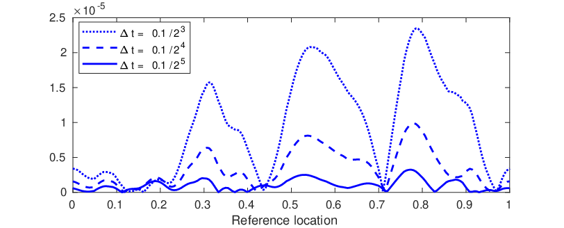
Figure 4 shows the point-wise linear convergence of the interior and exterior traction to Γh~\Gamma_{\tilde{h}}. The traction is computed at the midpoint of each segment of Γh~\Gamma_{\tilde{h}}, corresponding to sj+12s_{j+\frac{1}{2}} in the reference configuration because the normal vector is not well-defined at each vertex of the polygon Γh~\Gamma_{\tilde{h}}. In each plot the traction at t=0.1t=0.1 computed using Δ​t=0.1/26\Delta t=0.1/2^{6} is compared to the traction computed using Δ​t=0.1/23\Delta t=0.1/2^{3}, Δ​t=0.1/24\Delta t=0.1/2^{4}, and Δ​t=0.1/25\Delta t=0.1/2^{5}. Each line shows the sum of the absolute value of the difference in each component of the traction vector at each point sj+12s_{j+\frac{1}{2}} in the reference configuration. Similarly, Figure 5 shows the linear convergence in interface location. The interface location at t=0.1t=0.1 computed using Δ​t=0.1/26\Delta t=0.1/2^{6} is compared to the traction computed using Δ​t=0.1/23\Delta t=0.1/2^{3}, Δ​t=0.1/24\Delta t=0.1/2^{4}, and Δ​t=0.1/25\Delta t=0.1/2^{5}. The sum of the absolute value of the difference in each coordinate 𝐗⁡(sj,0.1){\bf X}(s_{j},0.1) is plotted.

Refer to caption
(a) Interior traction.
Refer to caption
(b) Exterior traction.
Figure 4: The above figure shows the convergence of the traction at t=0.1t=0.1 to the true solution computed using Δ​t=0.1/26\Delta t=0.1/2^{6}, μ=0.1\mu=0.1, and κ=1\kappa=1. The initial interface configuration is that described in Example 2. The quantity plotted is the sum of the absolute value of the difference at each midpoint on Γh~\Gamma_{\tilde{h}}. Point-wise convergence of the interior and exterior traction is observed.
Refer to caption
Figure 5: Plot of the difference between the interface location at t=0.1t=0.1 computed using Δ​t=0.1/26\Delta t=0.1/2^{6} and the time steps indicated in the plot with μ=0.1\mu=0.1 and κ=1\kappa=1. The initial interface configuration is that described in Example 2. The quantity plotted is the sum of the absolute value of the difference at each midpoint on Γh~\Gamma_{\tilde{h}}.
Table 3: Temporal convergence rates rΔ​tr_{\Delta t} using Richardson extrapolation for Example 2 (ellipse) and Example 3 (heart) with μ=1\mu=1 and κ=10\kappa=10. The results in from this test indicate linear convergence of velocity 𝒖\bm{u} in the L2L^{2} norm when using the semi-implicit method.

Δ​t\Delta t

0.1 0.1/2 0.1/220.1/2^{2} 0.1/230.1/2^{3} 0.1/240.1/2^{4}
Ellipse 1.5094 1.7405 1.9461 1.5505 -
Heart 3.7075 2.3262 - 4.7735 1.2742

5.3 Example 3: Heart

The third example is used to ensure that energy stability still holds regardless of the convexity of the interface and displacement of the centroid of the interior subdomain. The original curve is constructed as the sum of two translated cardioids and is parameterized by s∈[0,1]s\in[0,1] as follows:

𝐗0​(s)=120​[cos⁡(2​π​s)​(7​(1−sin⁡(2​π​s))+3​(1−cos⁡(2​π​s)))+24sin⁡(2​π​s)​(3​(1−sin⁡(2​π​s))+7​(1−cos⁡(2​π​s)))+24].{\bf X}^{0}(s)=\frac{1}{20}\begin{bmatrix}\cos(2\pi s)\left(7(1-\sin(2\pi s))+3(1-\cos(2\pi s))\right)+24\\ \sin(2\pi s)\left(3(1-\sin(2\pi s))+7(1-\cos(2\pi s))\right)+24\end{bmatrix}.

The energy plots in Figure 6 show that the energy in the explicit method becomes unstable slower than in the previous example. However, the semi-implicit method remains stable. Figure 7 shows the position of the interface as it deforms and moves toward the top-right corner of Ω\Omega, approaching a circular steady state. In this figure we observe a quick deformation to a convex interior at t=0.05t=0.05 and a translation of this region in the subsequent time steps. Table 4 shows the normalized deviation from the original interior area at time t=0.5t=0.5. Contrary to the previous example, we see more improvement from reduction of Δ​t\Delta t than from refinement of hh. Here, the area loss is reduced almost linearly with the reduction in Δ​t\Delta t and very little corresponding to a smaller mesh size hh.

Refer to caption

Figure 6: Plot of the energy of the system in Example 3, comparing the explicit and semi-implicit methods with μ=1\mu=1, κ=6\kappa=6, N=32N=32, and Δ​t=0.05\Delta t=0.05 (□\square for explicit, ∘\circ for semi-implicit) or Δ​t=0.01\Delta t=0.01 (∗* for explicit, ×\times for semi-implicit). The lines connecting data points are included when plotting the results of the explicit method to highlight the steep increase in energy.
Refer to caption
Figure 7: Plot of the position of the interface shown at t=0t=0, t=0.05t=0.05, and t=1t=1. Simulation run with μ=0.01\mu=0.01, κ=50\kappa=50, N=32N=32, Δ​t=0.01\Delta t=0.01, and initial configuration from Example 3.
Table 4: Normalized deviation of interior area at t=0.5t=0.5 from initial interior area in Example 3. Results obtained using μ=1\mu=1 and κ=10\kappa=10 with Δ​t\Delta t and hh as shown.

Δ​t\Delta t

2.5e-3 1.25e-3 6.25e-4 3.125e-4
16 4.3740e-03 2.3318e-03 1.2818e-03 7.7174e-04
1/h1/h 32 5.1529e-03 2.8014e-03 1.4961e-03 8.0600e-04
64 5.0489e-03 2.7171e-03 1.4206e-03 7.3541e-04

In Table 3 the temporal convergence of the velocity in the L2L^{2} norm is estimated using Richardson extrapolation alongside the rate of convergence estimates for the previous example. One can see that the rate of convergence is super-linear both examples.

Figure 8 shows the point-wise convergence of the interior and exterior traction. The traction is evaluated at the midpoint of each segment of Γh~\Gamma_{\tilde{h}} and the quantity plotted is analogous to that described in the previous example. Figure 5 shows the convergence of the interface at t=0.1t=0.1 using refined values of Δ​t\Delta t compared to the interface location at t=0.1t=0.1 using Δ​t=0.1/26\Delta t=0.1/2^{6}.

Refer to caption
(a) Interior traction.
Refer to caption
(b) Exterior traction.
Figure 8: The above figure shows the convergence of the traction at t=0.1t=0.1 to the true solution computed using Δ​t=0.1/26\Delta t=0.1/2^{6}, μ=10\mu=10, and κ=1\kappa=1. The initial interface configuration is that described in Example 3. The quantity plotted is the sum of the absolute value of the difference at each point midpoint on Γh~\Gamma_{\tilde{h}}. Point-wise convergence of the interior and exterior traction is observed.
Refer to caption
Figure 9: Plot of the difference between the interface location at t=0.1t=0.1 computed using Δ​t=0.1/26\Delta t=0.1/2^{6} and the time steps indicated in the plot with μ=10\mu=10 and κ=1\kappa=1. The initial interface configuration is that described in Example 3. The quantity plotted is the sum of the absolute value of the difference at each point midpoint on Γh~\Gamma_{\tilde{h}}.

5.4 Example 4: Stretched circle

The fourth example is chosen to emphasize the effects of a nonuniform tension around the perimeter of Γh~0\Gamma_{\tilde{h}}^{0}. The initial configuration is a circle of radius 14\frac{1}{4} centered at (12,12)\left(\frac{1}{2},\frac{1}{2}\right) with its parameterization given by

(27) 𝐗0​(s)=14​[cos⁡(2​π​s)+2sin⁡(2​π​s)+2],s∈[0,1].{\bf X}^{0}(s)=\frac{1}{4}\begin{bmatrix}\cos(2\pi s)+2\\ \sin(2\pi s)+2\end{bmatrix},\quad s\in[0,1].

Previously we chose equally-spaced points from the interval [0,L][0,L] when the tension of each segment was arbitrary. Since Γh~0\Gamma_{\tilde{h}}^{0} is a circle, we must sample at nonuniform sjs_{j} to prescribe a nonuniform tension on the edges of the polygon Γh~0\Gamma_{\tilde{h}}^{0}. The parameter values s~j\tilde{s}_{j} used to compute 𝐗j0=𝐗0​(s~j){\bf X}_{j}^{0}={\bf X}^{0}(\tilde{s}_{j}) are the m+1m+1 evenly spaced points sj∈[0,1]s_{j}\in[0,1] mapped by the cubic function

s~j=15​(16​sj3−24​sj2+13​sj).\tilde{s}_{j}=\frac{1}{5}\left(16s_{j}^{3}-24s_{j}^{2}+13s_{j}\right).

The result of this simulation, computed using the semi-implicit method, will be a leftward moving circle as a force tangent to the interface is applied to the fluid. Equilibrium is obtained when the points on the circle are equally spaced and the total force applied to the fluid is zero. Figure 10 shows the position of the points on the interface at three time steps. These plots highlight the leftward motion and the even distribution of the points on Γh~n\Gamma_{\tilde{h}}^{n} near steady state, at t=1t=1. In this example, the semi-implicit method is unconditionally stable.

Refer to caption

Figure 10: Position of the interface at t=0t=0, t=0.05t=0.05, and t=1t=1. We let μ=1\mu=1, κ=10\kappa=10, Δ​t=0.01\Delta t=0.01, and N=32N=32 and use the initial configuration from Example 4. An encircled red ×\times is used to denote 𝐗⁡(s0,t){\bf X}(s_{0},t) for reference. We display every 6th point on the interface to reduce clutter.

6 Conclusions

In this work we presented a new finite element method for solving unsteady Stokes equations with an immersed membrane that moves with the velocity of the fluid, not known a priori. We successfully combined the classical immersed boundary method with Nitsche’s formulation and CutFEM to solve this problem in two dimensions. The proposed method maintains the use of the Dirac delta function to pass the force applied by the immersed structure in the Lagrangian frame to the fluid in the Eulerian frame. more accurately incorporating the force applied by the interface on the fluid with conditional energy stability. We developed a semi-implicit discretization and added the necessary consistent penalty terms to maintain energy stability. The stability of our method is proved and verified in each example of our numerical results. This semi-implicit method was tested alongside the explicit CutFEM method, which is the algorithm directly analogous to the original finite element immersed boundary method [5]. Using CutFEM we improved the error in computing the velocity and pressure of the fluid near the interface; however, we continued the use of a polygonal approximation to the interface for its simplicity in computing the location of Γh~n+1\Gamma^{n+1}_{\tilde{h}}.

The numerical results demonstrate that if the polygonal approximation to the interface is refined as the mesh is refined, we obtain optimal spatial convergence in Example 1, as shown in Table 1. We also observe in Examples 2-4 the theoretical unconditional energy stability proved in this work. The conservation of area in each subdomain is desired and obtained for sufficiently small values of hh and Δ​t\Delta t. The trends observed in Table 2 and Table 4 are seen for sufficiently small values of Δ​t\Delta t. For larger values of Δ​t\Delta t we see an improvement in area conservation as Δ​t\Delta t is refined, however we may not observe such trends as hh is reduced.

References

  • [1] Slimane Adjerid, Mohamed Ben-Romdhane, and Tao Lin. Higher degree immersed finite element methods for second-order elliptic interface problems. Int. J. Numer. Anal. Model., 11(3):541–566, 2014.
  • [2] G. Agresar, J.J. Linderman, G. Tryggvason, and K.G. Powell. An adaptive, Cartesian, front-tracking method for the motion, deformation and adhesion of circulating cells. J. Comput. Phys., 143:346–380, 1998.
  • [3] Eberhard Bänsch. Finite element discretization of the Navier-Stokes equations with a free capillary surface. Numer. Math., 88(2):203–235, 2001.
  • [4] R. Becker, E. Burman, and P. Hansbo. A Nitsche extended finite element method for incompressible elasticity with discontinuous modulus of elasticity. Comput. Methods Appl. Mech. Engrg., 198:3352–3360, 2009.
  • [5] Daniele Boffi and Lucia Gastaldi. A finite element approach to the immersed boundary method. Comput. Struct., (81):491–501, 2003.
  • [6] Daniele Boffi, Lucia Gastaldi, and Luca Heltai. Numerical stability of the finite element immersed boundary method. Math. Models Methods Appl. Sci., 17(10):1479–1505, 2006.
  • [7] Daniele Boffi, Lucia Gastaldi, Luca Heltai, and Charles Peskin. On the hyper-elastic formulation of the immersed boundary method. Comput. Methods Appl. Mech. Engrg., 197:2210–2231, 2008.
  • [8] E. Burman and M. Fernández. Stabilization of explicit coupling in fluid-structure interaction involving fluid incompressibility. Comput. Methods Appl. Mech. Engrg., 198(5-8):766–784, 2009.
  • [9] Erik Burman. Ghost penalty. C.R. Math. Acad. Sci. Paris, 348(21-22):1217–1220, 2010.
  • [10] Erik Burman, Susanne Claus, Peter Hansbo, Mats G. Larson, and André Massing. CutFEM: Discretizing geometry and partial differential equations. Int. J. Numer. Meth. Engrg., 104(7):472–501, 2014.
  • [11] Erik Burman, Johnny Guzmán, Manuel A. Sánchez, and Marcus Sarkis. Robust flux error estimation of Nitsche’s method for high contrast interface problems, 2016.
  • [12] Erik Burman and Peter Hansbo. Fictitious domain finite element methods using cut elements: I. A stabilized Lagrange multiplier method. Comput. Methods Appl. Mech. Engrg., 199(41-44):2680–2686, 2010.
  • [13] Erik Burman and Peter Hansbo. Fictitious domain finite element methods using cut elements: II. A stabilized Nitsche method. Applied Numerical Mathematics, 62:328–341, 2012.
  • [14] J. Chessa and T. Belytschko. An extended finite element method for two-phase fluids. J. Appl. Mech., 70:10–17, 2003.
  • [15] Yan Gong, Bo Li, and Zhilin Li. Immersed-interface finite-element methods for elliptic interface problems with nonhomogeneous jump conditions. SIAM J. Numer. Anal., 46(1):472–495, 2007/2008.
  • [16] Yan Gong and Zhilin Li. Immersed interface finite element methods for elasticity interface problems with non-homogeneous jump conditions. Numer. Math. Theory Methods Appl., 3(1):23–39, 2010.
  • [17] Sven Gross and Arnold Reusken. Numerical methods for two-phase incompressible flows, volume 40 of Springer Series in Computational Mathematics. Springer-Verlag, Berlin, 2011.
  • [18] Johnny Guzmán and Maxim Olshanskii. Inf-sup stability of geometrically unfitted Stokes finite elements, 2016.
  • [19] Johnny Guzmán, Manuel A. Sánchez, and Marcus Sarkis. On the accuracy of finite element approximations to a class of interface problems. Math. Comp., 85:2071–2098, 2016.
  • [20] Johnny Guzmán, Manuel A. Sánchez, and Marcus Sarkis. A finite element method for high-contrast interface problems with error estimates independent of contrast. J. Sci. Comput., 73(1):330–365, 2017.
  • [21] Peter Hansbo. Nitsche’s method for interface problems in computational mechanics. GAMM-Mitteilungen, 28(2):183–206, 2005.
  • [22] Peter Hansbo, Mats G. Larson, and Sara Zahedi. A cut finite element method for a Stokes interface problem. Appl. Numer. Math., 85:90–114, 2014.
  • [23] Peter Hansbo, Mats G. Larson, and Sara Zahedi. A cut finite element method for coupled bulk-surface problems on time-dependent domains. Comput. Methods Appl. Mech. Engrg., 307:96–116, 2016.
  • [24] Xiaoming He, Tao Lin, and Yanping Lin. Immersed finite element methods for elliptic interface problems with non-homogeneous jump conditions. Int. J. Numer. Anal. Model., 8(2):284–301, 2011.
  • [25] Xiaoming He, Tao Lin, and Yanping Lin. The convergence of the bilinear and linear immersed finite element solutions to interface problems. Numer. Methods Partial Differential Equations, 28(1):312–330, 2012.
  • [26] Qingguo Hong and Johannes Kraus. Uniformly stable discontinuous Galerkin discretization and robust iterative solution methods for the Brinkman problem. SIAM J. Numer. Anal., 54(5):2750–2774, 2016.
  • [27] Ming Chih Lai and Zhilin Li. A remark on jump conditions for the three-dimensional Navier-Stokes equations involving an immersed moving membrane. Applied Math. Letters, 14:149–154, 2001.
  • [28] Raytcho Lazarov and Aziz Takhirov. A note on the uniform inf-sup condition for the Brinkman problem in highly heterogeneous media. J. Comput. Appl. Math., 340:537–545, 2018.
  • [29] R. J. Leveque and Zhilin Li. The immersed interface method for elliptic equations with discontinuous coefficients and singular sources. SIAM J. Numer. Anal., 31(4):1019–1044, 1994.
  • [30] R. J. Leveque and Zhilin Li. Immersed interface methods for Stokes flow with elastic boundaries or surface tension. SIAM J. Sci. Comput., 18(3):709–735, 1997.
  • [31] Zhilin Li, Tao Lin, and Xiaohui Wu. New Cartesian grid methods for interface problems using the finite element formulation. Numer. Math., 96(1):61–98, 2003.
  • [32] Tao Lin, Yanping Lin, and Xu Zhang. Partially penalized immersed finite element methods for elliptic interface problems. SIAM J. Numer. Anal., 53(2):1121–1144, 2015.
  • [33] Kent Andre Mardal, Xue-Cheng Tai, and Ragnar Winther. A robust finite element method for Darcy-Stokes flow. SIAM J. Numer. Anal., 40(5):1605–1631, 2002.
  • [34] Kent-Andre Mardal and Ragnar Winther. Uniform preconditioners for the time dependent Stokes problem. Numer. Math., 98(2):305–327, 2004.
  • [35] André Massing, Mats G. Larson, Anders Logg, and Marie E. Rognes. A stabilized Nitsche fictitious domain method for the Stokes problem. Journal of Scientific Computing, 61:604–628, 2014.
  • [36] Elijah P. Newren, Aaron L. Fogelson, Robert D. Guy, and Robert M. Kirby. Unconditionally stable discretizations of the immersed boundary equations. J. Comput. Phys., 222:702–719, 2007.
  • [37] J. Nitsche. Über ein variationsprinzip zur lösung von dirichlet-problemen bei verwendung von teilräumen, die keinen randbedingungen unterworfen sind. Abh. Math. Sem. Univ. Hamburg, 36:9–15, 1970/71.
  • [38] Charles S. Peskin. Numerical analysis of blood flow in the heart. J. Comput. Phys., 25(3):220–252, 1977.
  • [39] Charles S. Peskin. The immersed boundary method. Acta Numerica, pages 479–517, 2002.
  • [40] Charles S. Peskin and D.M. McQueen. A three-dimensional computational method for blood flow in the heart. I. immersed elastic fibers in a viscous incompressible fluid. J. Comput. Phys., 105(1):372–405, 1989.
  • [41] C. Tu and C.S. Peskin. Stabiity and instability in the computation of flows with moving immersed boundaries: a comparison of three methods. SIAM J. Sci. Statist. Comput., 13:1361–1376, 1992.
  • [42] Xiaoping Xie, Jinchao Xu, and Guangri Xue. Uniformly-stable finite element methods for Darcy-Stokes-Brinkman models. J. Comput. Math., 26(3):437–455, 2008.