Metastable transitions in inertial Langevin systems: what can be different from the overdamped case?
Abstract
Metastable transitions in Langevin dynamics can exhibit rich behaviors that are markedly different from its overdamped limit. In addition to local alterations of the transition path geometry, more fundamental global changes may exist. For instance, when the dissipation is weak, heteroclinic connections that exist in the overdamped limit do not necessarily have a counterpart in the Langevin system, potentially leading to different transition rates. Furthermore, when the friction coefficient depends on the velocity, the overdamped limit no longer exists, but it is still possible to efficiently find instantons. The approach we employed for these discoveries was based on (i) a simple rewriting of the Freidlin-Wentzell action in terms of time-reversed dynamics, and (ii) an adaptation of the string method, which was originally designed for gradient systems, to this specific non-gradient system.
Keywords:
Freidlin-Wentzell large deviation theory, instanton, inertial Langevin equation, underdamped dynamics, matrix-valued variable friction coefficient.1 Introduction
The Langevin equation
can exhibit richer behaviors than its overdamped limit
| (3) |
where is a positive definite mass matrix, is a positive definite friction coefficient matrix, the variables , , and is an -dimensional Wiener process. When the equations are deterministic and play a special role in the limit. We also refer to the case by the same names, but when ambiguity arises we will add the term “noiseless" to distinguish the two cases.
Let denote a weighted norm,
| (4) |
where and is a positive definite matrix. Freidlin-Wentzell theory shows the transition from one point in the state space to another of 1 or 3 is characterized by the minimizer of the following actions
| (5) |
and
| (6) |
The minimizers of these functionals are often called instantons. They give a higher order correction to the leading order approximation of noiseless dynamics, taking into account the long-term effects of small noise.
Of particular interest is when is the gradient of a potential, i.e. for a function . Suppose one is interested in the transition from a local minimum of to a saddle point . If there exists a heteroclinic connection from to in the noiseless overdamped system as well as a heteroclinic connection in a modification of the noiseless Langevin system, then the values of the functionals 5 and 6 coincide; see §2. Furthermore, the existence of a heteroclinic connection in the former system does not guarantee the existence for a counterpart in the latter. As we will see in §4.2, if the friction coefficient is sufficiently low, the correspondence between these two heteroclinic connections can be broken. This implies that the minimal values of the two functionals no longer need to coincide. More generally, if the friction coefficient matrix has at least one sufficiently low eigenvalue, this possibility exists.
Consequently, the minimizing paths themselves can also be markedly different between the overdamped limit and the Langevin equation. This is no surprise given that the overdamped limit of the Langevin equation is a reversible diffusion process governed by a gradient system whereas the inertial Langevin system is irreversible, non-gradient, and non-uniformly-elliptic. We will describe how to compute the Langevin instantons in §3, based on structures of the functionals 5 and 6 illustrated in §2. It is oftentimes possible to leverage computations from the overdamped equation to obtain instantons for the Langevin functional, and the string method [3, 4] originally designed for overdamped Langevin only needs to undergo a slight change to adapt to a matrix-valued friction coefficient that depends on position and velocity. However, for reasons just mentioned, it is still possible to miss local minimizers of the action 5, and when this happens, we resort to the first-order optimality condition, which is only utilized in §4.2 for understanding the differences between underdamped and overdamped Langevin equations.
§4 discusses the details of the Langevin transition problem in cases, with increasing complexity based on different kinds of positive definite friction coefficient matrices:
- 1.
- 2.
Constant Underdamped. When the eigenvalues of the friction coefficient matrix are sufficiently low, new phenomena distinctive from the overdamped limit can arise in the Langevin system. Physically this case may be motivated by considering situations where inertial effects are important. Fundamental differences appear when heteroclinic connections in the overdamped limit have no analog in the corresponding Langevin equation. Additionally, it is no longer the case that the global minimizer of the Freidlin-Wentzell action is a “time-reversed" trajectory. We first illustrate this using a standard 4-dimensional test problem and then provide an explanation based on semi-analytical understanding of a 2-dimensional example in §4.2. Note that there have been great work on friction approaching zero asymptotics (e.g., [8, 9]), and the scope of this article is complementary as we focus on finite friction coefficients and masses.
- 3.
Position Dependent. In addition we analyze position dependent friction coefficient matrices. See [10] and references therein for why such frictions are worth studying. Another motivation for position-dependent friction is to model certain biological systems – when interactions with a solvent are modeled by noise and friction, the hydrophobic and hydrophilic regions of lipid bilayer, for instance, correspond to different friction coefficients [11].
To illustrate what difference can be induced by the position dependence, we give an example in §4.3, where we see that a localized change in the friction coefficient at a critical location can lead to a global change in the instanton. Two different definitions of an overdamped ‘limit’ will also be discussed — one preserves the invariant distribution of Boltzmann-Gibbs, and the other is consistent in terms of rare events.
- 4.
Velocity Dependent: The structure of the Langevin functional also allows for the consideration of (both position and) velocity dependent friction coefficients, even though there is no more overdamped limit and Boltzmann-Gibbs is in general no longer an invariant distribution either. Velocity dependent friction coefficient can be viewed as a more flexible model of friction allowing for deviations from linear models [12, 13]. The long term goal is to be able to address more complicated frictions such as those used to model swarming (e.g., [14, 15]) and astrophysical dissipation (e.g., [16, 17]), but investigations in this article are restricted to cases when zero velocity corresponds to stable fixed points or saddles.
To correctly compute instantons in the presence of velocity dependent friction coefficient (i.e., friction nonlinear in velocity), modifications need to be made. In particular, if the friction is not symmetric with respect to sign change in velocity, one has to consider two Langevin-type systems. See §3.1 and §4.4.
There are many great surveys of how to find minimizing trajectories in dynamical systems with noise, and here we provide an incomplete list of two most recent ones, [18] and [19]. The Langevin system considered here may be understood formally via a transverse decomposition of a first-order system (see [20] and additionally [21]), however the noise is degenerate (i.e., non-uniformly-elliptic diffusion). Versatile numerical methods based on action minimization such as [22, 23, 24, 25, 26, 27, 28, 29, 18] work for nongradient systems and infinite dimensional systems too, but their applications to our system require adaptations, also due to the degenerate noise. Powerful theories based on hypoellipticity [30, 31] and hypocoercivity [32] do provide tools for analyzing the degenerate and irreversible (but not too irreversible) system of Langevin, but our simple theoretical derivation will not require them.
2 Problem Formulation
In order to simplify analysis of the Langevin equation, we first change to mass coordinates, as in [33], , , , , so that
| (7) |
becomes
The correlation matrix is , thus we may effectively replace this system by
without changing relevant statistics. In these coordinates we have a system of identity mass with effective friction coefficient . In this regard low mass and high friction are similar. Thus, with this rescaling in mind, we take mass to be the identity matrix from now on.
Although the global minimizers of functionals 5 and 6 are the only ones relevant for the most likely transitions, we relax this requirement and compute local minimizers. The rationale is that local minimizers are often associated to dynamical structures such as saddle points (see (12) and (13) and discussions that follow), and if one can exhaust these structures (this is often easier), all local minimizers and hence the global one, can be found. We are interested in the case where the position boundary conditions coincide for the minimization of the overdamped and Langevin functionals, , , and the Langevin functional minimization is augmented with additional velocity boundary conditions, , . We typically choose homogeneous velocity boundary conditions, .
Utilizing the identity we rewrite the functionals 5 and 6 as follows,
| (12) |
and
| (13) |
These calculations show that the functionals are bounded below, i.e.
| (14) | ||||
| (15) |
and in particular the lower bounds coincide if .
The two main cases that we focus on here are
- 1.
The transition from a saddle point to a local minimum of , with velocity boundary conditions , abbreviated .
- 2.
The transition from a local minimum to a saddle point of , with velocity boundary conditions , abbreviated .
The velocity and position boundary conditions guarantee that we are considering transitions between fixed points in both the Langevin and overdamped case. From this point on we consider the limit.
In the former case, if there exists a heteroclinic connection in the deterministic dynamics (for both systems) from to then the minimum action is , since the minimizer is exactly given by deterministic dynamics (in the infinite time limit), i.e.
| (16) | ||||
| (17) |
However, it is possible for heteroclinic connections that exist in 17 to not exist in 16 and vice versa as we show in §4.2.
For it is also possible to find the minimizing trajectory which achieves equality in 14 and 15. We first focus on the case where depends only on position and assume that there exists a heteroclinic connection from to in the following systems:
| (18) | ||||
| (19) |
In this case, these connections are the action minimizing trajectories. Reversing time , and denoting derivatives with respective to the new variable with ′, i.e. , we see
| (20) | ||||
| (21) |
which are exactly the same as 16 and 17 with respect to the new variables. The minimizing trajectory becomes the same as the noiseless trajectory from after a sign change of the velocity variable in the Langevin case.
If the friction coefficient matrix depends on velocity then the minimizing trajectory must satisfy
| (22) |
which only coincides with 16 if . We call 22 the time-reversed Langevin equation. Heteroclinic connections that exist in 18 do not necessarily exist in 22.
If there is no heteroclinic connection between points of phase space, the time-reversed dynamics do not correspond to minimizers. To understand this case better, we directly use the Euler-Lagrange equation of the variational principle (note: the appearance of normally would require the introduction of a jet bundle instead of the standard tangent bundle, but there is no need to concern this technicality because we work with flat position space ):
| (23) | ||||
| (24) |
If the friction coefficient matrix is isotropic then simplifications occur for the Langevin functional 5 and the Euler-Lagrange equation becomes
| (25) |
We solve this boundary value problem numerically: §3.3 uses gradient descent, a finite time-horizon approximation, and pseudospectral discretization.
3 Numerical Methods
To compute minimizers to the Freidlin-Wentzell action 5, we utilize three different methods: the string method, the numerical integration of dynamics, and directly solving the boundary value problem. We review each method and show how to implement them in the following subsections. Their use in practice is illustrated in §4.
3.1 String method
The string method is both a way of locating saddles between local minima as well as a way to approximate local minimizers of the overdamped Freidlin-Wentzell action [3], [4]. To utilize this method one proceeds as follows:
- 1.
First define an initial “string", i.e, a sequence of points from one local minimum to another, or simply a sequence of points that lie across a separatrix. For example, in many cases one can choose a straight line between one local minimum and another.
- 2.
Evolve each point on the string according to the deterministic dynamics for a single time-step.
- 3.
Calculate the total length of the string and then evenly redistribute the set of points on the string.
- 4.
Repeat 2-3 until convergence.
The path interpolated by the sequence of points (also called images) is the “string".
The string method can also be applied to the Langevin system by writing the equation as a first order system. Furthermore it can approximate a local minimizer of the corresponding Langevin Freidlin-Wentzell action by making a few adaptations. As stated in the previous section, once a saddle is located, the minimizer of the Freidlin-Wentzell action from a local minimum to a saddle obeys time-reversed dynamics, i.e.
as long as a heteroclinic connection exists from the minimum to the saddle. Reversing time, and making the change of variables , yields the following system
where . This is the noiseless Langevin equation, but with friction coefficient matrix as opposed to . If the friction coefficient matrix is an even function of the velocity then one can run the string method without modification to compute the correct positions of the string. Once the string has converged, the velocity terms need to undergo a sign flip in the “uphill" part of the string.
We illustrate what we mean by the sign flip in Figure 1. Here we are computing the transition path in the double well potential
| (30) |
from to for . There is a saddle at the point and it serves as the partition from “uphill" to “downhill". The true action minimizing path may be viewed as going “uphill" from to and then proceeding “downhill" along dynamics from to . The left most figure is obtained by evolving a string; however, this is not the action minimizing path. Along the uphill part, from to , the velocity variable needs to be multiplied by a negative sign to produce the true action minimizing path. Doing so the middle figure is obtained. The rightmost figure is the action minimizing path obtained as a solution to the Euler-Lagrange equations 25, via the methods of §3.3.

If , the procedure needs to be modified. We illustrate this with the following (noiseless) system:
Here the nonlinear friction coefficient is . The easiest solution is to evolve two strings. The first obeys the noiseless Langevin dynamics (as in 3.1) and the latter obeys 3.1. With regards to 3.1 the corresponding time-reversed system is
where the the nonlinear friction coefficient is . We call this system the time-reversed (noiseless) Langevin equation. The instanton is then a concatenation of different halves (separated by the saddle point) of these two different strings. For the uphill part one takes the string for the time-reversed Langevin equation with a sign flip on velocity and for the downhill part one takes the Langevin string. For example, in Figure 2 the two systems, 3.1 and 3.1, are simulated via the string method in the top two panels. The instanton for the system for two different transitions– to and to –are shown in the bottom two panels. The to transition is constructed by taking the to half of the string corresponding to 3.1 (downhill dynamics), and concatenating it with the to half of the time-reversed system with velocity multiplied by a negative sign (uphill trajectory). An analogous procedure is used to construct the to transition.

It is important to keep in mind that the string method can only compute a local minimizer of the Freidlin-Wentzell action, and different initializations of the string could give rise to different local minimizers. On a practical level, one can try different string initializations and choose the final string that best minimizes the Freidlin-Wentzell action.
3.2 Saddle points and dynamics
The Langevin instantons are generally more costly to compute than the overdamped case as they can be more oscillatory. For instance, the method described in §3.1 often under-resolves the instanton unless it is discretized by a large number of points. To reduce the computational cost, knowledge of the overdamped dynamics (when they exist) can be exploited. Such knowledge includes, in particular, the saddle point and the perturbation directions off that saddle to the local minima. A sufficiently resolved string produces the minimizing path for the overdamped system, which includes the approximate location of a saddle between two minima as well as the perturbation directions. We mention that if one is purely interested in just the saddle, the computation of the string can be avoided, see for example [34, 35].
When both heteroclinic connections exist (see §2), we utilize these approximate perturbation directions of the overdamped system to obtain approximate perturbation directions of the Langevin system and run dynamics to compute the instanton.
This algorithm proceeds as follows:
- 1.
Calculate the overdamped string.
- 2.
Locate the saddle(s), and then utilize perturbations away from the saddle (as calculated by the string) to obtain perturbation directions for the inertial Langevin system.
- 3.
Simulate the dynamics of the corresponding noiseless Langevin equations. Concatenate to construct the instanton.
One way to locate a saddle point on a string is to evaluate the norm of the force at each point on the string and choose the one with . If heteroclinic connections exist, it is possible to explicitly calculate the correct perturbation direction off the saddle for the Langevin system based on the overdamped result, see §A. Another possibility is to compute underresolved Langevin strings (i.e. those in §3.1) for approximating the perturbation directions.
3.3 Euler-Lagrange equation
It is sometimes necessary to compute instantons directly by numerically solving the Euler-Lagrange equation. This is based on an iterative minimization of the Freidlin-Wentzell action analogous to existing results. In fact, great methods have been developed to compute local minima of 6 which can be nongradient. Among them include the minimum action method [22], adaptive minimum action method [23] and its higher-order version [24], the geometric minimum action method [25, 26, 27], and methods based off of dynamic programing [36]. It is also possible to utilize the Hamiltonian formulation, see [25, 18, 28]. Note, though, with regards to the Langevin problem considered here, there is no need to use these more generic and more costly approaches, unless the or heteroclinic connection does not exist (whether they exist is verifiable by methods in §3.1 and §3.2).
Action minimization methods have a natural extension to the Langevin setting 5. For example, one can use gradient-descent and a finite approximation to compute minimizers, similar to what was originally done with the minimum action method [22]. Due to the second derivatives arising in the functional, however, the resulting boundary value problem will be fourth-order. Specifically the Euler-Lagrange equations for the Langevin functional are
| (35) |
under the assumption that the friction coefficient matrix is isotropic, and identity mass.
As per usual with gradient-descent, we introduce pseudo-time and evolve
| (36) |
forward in pseudo-time until is sufficiently small. When discretizing pseudo-time we treat the linear terms implicitly in order to mitigate stiffness due to hyper-diffusion and diffusion, as is commonly done in numerical partial differential equations. Explicitly, the following linear update is solved at every time step
| (37) |
where is the pseudo-time step size. This is a linear boundary value problem for at every time-step.
Amongst the many methods to discretize time we utilize a modern form of spectral integration as in [37] and [38] . The main idea behind the method is to rewrite 37 in integral form and represent the solution utilizing Chebyshev polynomials. Although derivative operators are dense with respect to Chebyshev collocation points, integral operators in spectral space are banded. This leads to efficient and numerically robust evaluation of solutions. Products and convolutions are computed utilizing the pseudo-spectral method [39].
It is worth noting that one can also compute minimizers to the action
| (38) |
where is a large parameter. The advantange of utilizing this functional is that one can use the same methods that are applied to systems with non-degenerate noise; however, solving 38 leads to a stiff system of equations, resulting in expensive computations. When heteroclinic connections exist, the action minimizer coincides with that of a non-stiff version,
| (39) |
as can be made zero pointwise. However, this relaxation may not work if one of the two heteroclinic connections doesn’t exist (although when they both exist there is less need to iteratively minimize the action).
4 The Differences
In what follows we examine local minimizers of the Langevin action 5 with matrix-valued and possibly position and velocity dependent friction coefficient to highlight generic differences and similarities with its overdamped limit 6 and isotropic friction coefficients. At the end of each section we give generic recommendations on numerical methods.
4.1 Large friction coefficient
The overdamped case has been studied extensively as previously mentioned, (e.g. [5], [6], [7], [8]). We also note that the closely related problem of the small mass limit — which we saw in §2 is related to high friction via a rescaling of coordinates — has been analyzed, see e.g., [40, 10, 41, 42]. To recall the phenomenology concretely, we use an illustration based on the Mueller potential
| (40) |
where the parameters for are chosen the same as [4]. The minimizer here can be computed via the string method or utilizing dynamics.
Figure 3 shows the trajectories of two local minimizers of the Freidlen-Wentzell action with an isotropic (i.e. scalar) friction coefficient . We see that, after projecting to position space in the case of Langevin system, there is little difference in the trajectory of the Langevin equation and its overamped limit, except for a small amount of overshoot in the Langevin dynamics.
In the high friction scenario this agreement is generic. If is much larger than the spectral radius of the Hessian of in the domain of interest, the friction is high enough to justify the overdamped limit.
Recommendation
The general recommendation for this case is to focus on the overdamped limit, and the string method in its original form is a good choice for computing the instanton.

4.2 Small constant scalar friction coefficient
As we lower the friction coefficient, new situations may arise since inertial effects can now compete with the potential. We first illustrate this in the Mueller system and then provide a detailed analysis of a system with a sixth-order polynomial potential. The features mentioned here are generic and we have observed similar behavior in other systems.
We apply the method of §3.2 and §3.3 to various dissipation regimes of the Mueller system. When the friction becomes small but not too small, for instance in this case, oscillatory behaviors near minima are seen in the instanton (left panel of Figure 4). These oscillations can be intuitively understood as an inertial effect due to the fact that the particle cannot stop or take sharp turns instantaneously, unless a lot of noise is used. However, the topology of the transition remains the same as the overdamped instanton.
Further lowering the friction coefficient, for instance to , leads to a difference in the instanton and a dynamical trajectory. A generic dynamical trajectory settles to a different minimum, see the right panel of Figure 4. In this case, the particle has enough momentum to overcome intermediary minimum and ends up in another minimum of the potential. One may think that this means a better perturbation direction needs to be chosen for a correct departure from the saddle point; however, in this case we posit that there no longer exists a heteroclinic connection between the saddle and the original target minimum.

To understand this possibility of losing heteroclinic connection, let us consider a simpler, one degree-of-freedom example (the governing SDE is therefore 2D ), where the potential is given by a sixth-order polynomial
| (41) |
for are such that there are three local minima at positions and saddles . Furthermore . See Figure 5 for an example.
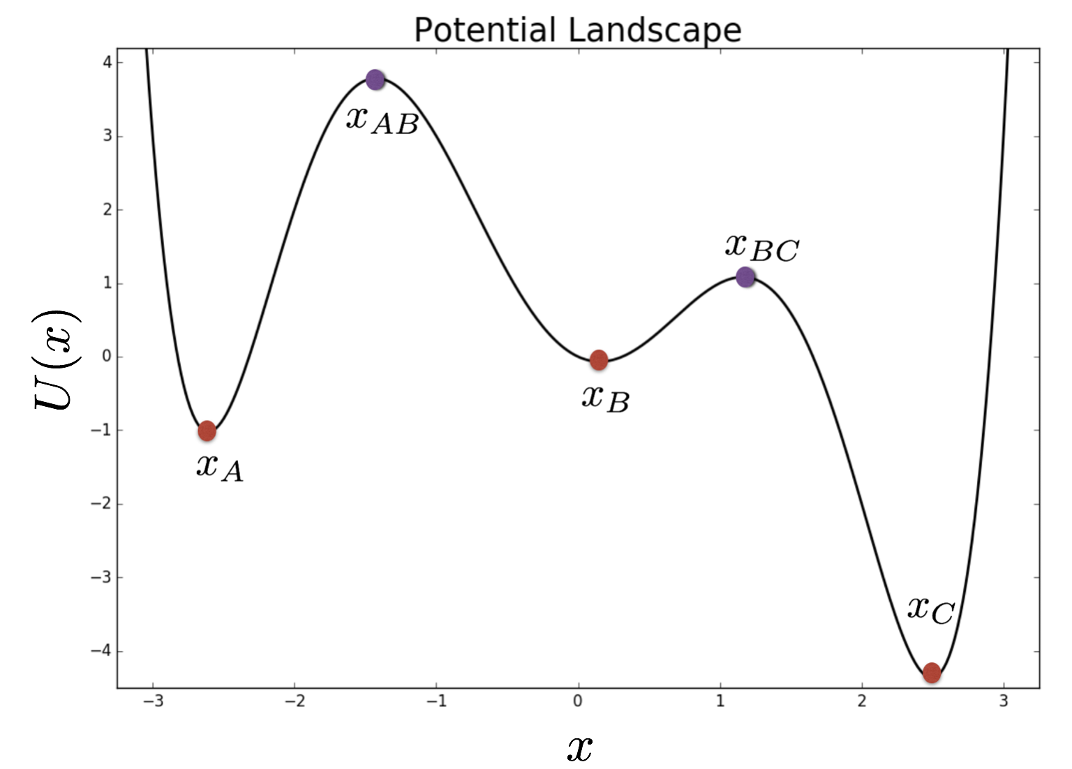
In the overdamped limit, the state space is 1-dimensional, and the transitions between different minima can only go through one path, i.e. the transition from has to first pass through the minima at . Furthermore the transitions must also pass through the saddles at and .
In the Langevin system, however, this is not necessarily the case since the state space is 2-dimensional. More precisely, the transition path of changes with the amount of friction in the system. With a large amount of friction, the transition simply passes through the saddle and slides into as a solution to 16; however with less friction 16 may no longer have an infinite time solution with boundary conditions and . Physically, this corresponds to the situation where the particle starts at the saddle with infinitesimal velocity to the right, builds up enough momentum due to insufficient friction, so that after passing it overcomes the small barrier given by and eventually settles at . In this case there is no dynamical path from , but there is a dynamical path from . Note with even less friction it is still possible for the heteroclinic connection from to to exist again (the particle can bounce back), but we focus on the case where this connection doesn’t exist. Naturally, this phenomenon of potential-well-skipping will be pronounced if .
There are three reasonable possibilities for the global action minimizer, when the boundary conditions are and (equipped with zero velocity) and yet there is no heteroclinic connection from to . The first corresponds to the dynamical paths / time-reversed paths , each equipped with zero velocity. In this case, the local minimal action value of the Freidlin-Wentzell action is
| (42) |
The second possibility corresponds to , but the instanton from to is no longer given by a simple deterministic dynamics. A more efficient minimizer of the action is obtained by deviating away from the deterministic path. The third possibility is that the minimizing path no longer transitions through the saddle and instead transitions from to directly, without passing through any other critical points.
Let us first compare the first two possibilities: in this example, it is more efficient to use noise to slow down the particle so that it settles at . Naturally, this is the case if the difference is sufficiently large, corresponding to a deep well at location . The first possibility is not optimal as the particle needs a lot of noise to crawl back into the well of , and it would rather spend a small amount of noise to slow down in the well of before getting trapped in the well of .
To be more specific, parameters used for producing Figure 5 are
so that
| (43) | ||||
| (44) |
and
In this case, when there exists a heteroclinic connection between and , whereas when there no longer exists a heteroclinic connection** * The gamma for which this bifurcation first occurs appears is between and .. Figure 7 shows the basins of attraction for the system, approximated by numerical simulations of a large amount of initial conditions. Zooming in close to one sees that the basin of attraction for had been eroded away, cutting off any noiseless transition from to .
The deterministic path, streamlines, and a minimizer of the Freidlin-Wentzell action (computed by the method in §3.3) for and are shown in Figure 6. One can see that the deterministic path corresponding to (going downhill from the point ) settles to the point , and the minimizer and the deterministic path coincide.

When the deterministic path ends up in the well corresponding to location whereas the local minimizer of the Freidlin-Wentzell action ends directly at . The action value for the minimizing path for the to transition is less than , meaning that the most likely transition from to does not go through , since this would correspond to an addition of to the action. The minimizer was found by solving the Euler-Lagrange equations via gradient descent (see §3.3). For this case all of our attempts to utilize the string method failed to produce the correct global minimizer. All sufficiently well resolved strings that we tried had at least one of its points in the basin of attraction of the well corresponding to . This seemed to be enough to sweep the rest of the string into a path that approximates the transition, a suboptimal local minimizer of the Friedlin-Wentzell action.

The third possibility, however, has not been theoretically ruled out. Nevertheless, our numerical computations of the transition were insufficient to show significant advantage of crossing the separatrix away from the saddle.
Recommendation
The first recommendation is to compute the overdamped string and then simulate deterministic dynamics §3.2. If the trajectories of the noiseless Langevin system end up in the same potential minima as was computed in the overdamped limit, then a good local minimizer of the action is found. If the trajectories end up in a potential minimum different from and , then plan B is to apply the adapted string method §3.1. If that again results in an insertion of an unwanted minimum in the middle of the transition (e.g., discussed above), the string method may have skipped a better action minimizer too. The last recourse then is to attempt to directly minimize the Freidlin-Wentzell action (see §3.3). This, of course, presents additional difficulties since it may be computationally expensive (depending on the structure of the problem).
4.3 Position dependent, matrix-valued friction coefficient
As the different effects of large and small scalar friction coefficients were described above, it is not difficult to see if the friction coefficient is a constant matrix with both small and (relatively) large eigenvalues, then a mixed effect can be induced by this anisotropy, which further complicates the transition. Details of the case of a constant but anisotropic friction coefficient will no longer be individually discussed for conciseness; instead, in this section we show that the anisotropy only needs to be a local effect in order to result in a global change in minimizing trajectories.
More precisely, consider an example with the potential
| (45) |
where . The friction coefficient matrix is
| (46) |
where , , and . The anistropy is local with respect to the friction coefficient, but notably occurs at a saddle point of the system — there the matrix is
| (47) |
whose eigenpairs are and . There is a large disparity between the two eigenvalues.

We consider the transition from to (again with zero velocities). If the friction coefficient is isotropic (i.e., a constant scalar), the minimizing trajectories of both the overdamped and the Langevin system stay on the line connecting and . The anisotropic position-dependent case is different. Utilizing the string method both adapted for the Langevin equation and for the overdamped equation leads to the scenarios in Figure 8. The computed local action minimizer for the overdamped string ends up going through additional potential minimum (e.g., ) and saddle points. On the other hand the Langevin string still goes directly from to without passing through additional minima.
Given that we cannot guarantee that the local minimizer for the overdamped functional is the global one, it is possible that a transition path that is more “direct" exists for this system, but the simple heteroclinic dynamics §3.2 do not exist. An approximation to the basin of attraction for the Langevin and overdamped system is shown in Figure 9. There we see that there is no heteroclinic connection from to in the noiseless overdamped system whereas it still exists Langevin system. At least two points are clear: (i) The straight line transition path, present when friction is isotropic, is no longer optimal due to the new friction, and (ii) overdamped transition and Langevin transition projected to position space may not coincide when friction coefficient is not uniformly large everywhere.

Recommendation
To numerically compute the instanton, here we give the same recommendation as in §4.2; however, caution should be used when one tries to compute a transition involving more than two minima by the string method: a large number of points might be needed to represent the string to avoid degraded accuracy due to under-resolution; one fix is to compute pairwise transitions between minima, and then concatenate. In addition, if one utilizes the Euler-Lagrange equation, 25 needs to be modified because it was for the scalar constant coefficient case, but now we have position-dependence.
Two overdamped limits
It is also important to clarify, in the position-dependent friction case, what is an overdamped limit of
| (48) |
We utilized the formal limit,
| (49) |
Repeating the derivation in §2, it is not difficult to see that, under the condition of existences of needed heteroclinic orbits, the formal limit 49 provides minimum action values consistent with those of the full system 48. Because of this, we used this formal limit to investigate the rare event of metastable transition.
Note, however, that this formal limit does not conserve the marginal of the Boltzmann-Gibbs distribution, , which however remains as an invariant distribution of the Langevin equation 48 despite the no-longer-constant friction coefficient. One can show, by solving the stationary Fokker-Planck equation, that the following corrected overdamped limit preserves the marginal Boltzmann-Gibbs,
| (50) |
where . This equation is in fact consistent with the variable friction small mass limit in the literature, and we refer to [10] for more discussions (including convergence of the dynamics, not just long term statistics) and references.
We chose not to further investigate rare events in this correction (49) though, because its large deviation structure is in fact unclear (one cannot simply remove the term via , since the noise also scales). An investigation could be interesting but it is out of the scope of this article. After all, our approach directly provided a solution to the full problem 48.
4.4 Velocity dependent, matrix-valued friction coefficient
Although complications previously investigated in 4.2 and 4.3 can all add up to this case, to avoid redundancy we concentrate on the differences that a velocity dependence can induce. We do so by revisiting the Mueller potential with an anisotropic velocity dependent friction coefficient matrix in a mildly underdamped situation. When the friction coefficient depends on velocity, generally there is no analogous overdamped limit any more, and the system
| (51) |
may not admit Boltzmann-Gibbs as an invariant distribution. In terms of nonequilibrium statistics, we show the velocity dependence modifies instantons.
More specifically, consider an example where only depends on , in the form of
| (52) |
Note ; thus we need to pay special attention to the time-reversed Langevin equation as well, see §2.
In Figure 10 we compute the same transition from §4.1, but with 52. Here there is a difference between time-reversed dynamics and regular Langevin dynamics since the friction coefficient matrix is not symmetric with respect to sign reversal of velocity. The true minimizing path, is a concatenation of the solid curves and the dashed curves. The string method or dynamics can still be utilized to compute the minimizing trajectory, but twice the computation is necessary.
The difference between time-reversed dynamics and regular dynamics can lead to significant complications. Given the phenomena in §4.2, heteroclinic connections that exist in
| (53) |
do not necessarily have an analog in
| (54) |

Recommendation
Even though there is no analogous overdamped limit, one can still utilize knowledge of the string in the overdamped limit to compute instantons for this system. To make use of the overdamped limit, use the friction coefficient matrix and compute the overdamped string. This is, in a general setup, a position-dependent-friction string calculation as in §4.3. Then one can use the method of dynamics §3.2 to compute trajectories for the Langevin equation and time-reversed Langevin equation. If the resulting noiseless (modified) Langevin trajectories do not end up at the target minimum, then one can also evolve two strings, one corresponding to Langevin dynamics and the other to the time-reversed dynamics, to compute a local action minimizer or obtain a better perturbation direction off the saddle. (Note that the method of obtaining an improved perturbation direction from the appendix is not always applicable to non-isotropic and non-constant friction coefficients.) If the previous methods fail and if it is feasible to do so, one can try to compute minimizers utilizing the Euler-Lagrange equations.
5 Conclusion
We analyzed minimizers of the Freidlin-Wentzell action for the inertial Langevin equation with respect to various types of friction coefficients, for illustrating features in inertial Langevin metastable transitions that differ from the familiar overdamped picture. We calculated local minimizers of the action functional utilizing three approaches, (i) an adaptation of string method, (ii) dynamics, and (iii) gradient descent minimization of the action, which not only depends on but also . We exploited the structure of the functional, which allows for a simple modification of the string method as well as an dynamics-based approach for improved resolution, provided heteroclinic connections exist. This structure also allows the calculation of instantons when the friction coefficient is position and/or velocity-dependent. When heteroclinic connections that exist for the overdamped system no longer correspond to that of the inertial system, we minimized the action directly, from whence we saw that instantons no longer need to obey dynamics or time-reversed dynamics. This implied that the minimum action values of the Langevin and overdamped functionals are different, leading to different transition rates.
6 Acknowledgment
MT is partially supported by NSF grant DMS-1521667 and ECCS-1829821 and AS is partially supported by DMS-1344199. MT is grateful for valuable discussions with Tony Lelièvre and encouragements from Jianfeng Lu to continue exploring this interesting problem. We also appreciate comments from two anonymous reviewers, which greatly improved the manuscript.
Appendix A Perturbation Direction
Suppose that is an eigenvector of the matrices with eigenvalues respectively. Then
| (55) |
is an eigenvector of the matrix
| (56) |
with eigenvalues
| (57) |
and
| (58) |
with appropriate modifications for the case. The derivation is as follows: Starting with the ansatz for the eigenvector we compute
| (59) |
and we choose the parameters and such that the diagonals of the matrix are equal.
With respect to the Langevin equation with a constant friction coefficient matrix , and Hessian of the potential , the Hessian of the Langevin system is the following block matrix
| (60) |
Assume that and the share an eigenvector , as for example would be the case for an isotropic friction coefficient. Based off of the previous calculations the eigenvector and values are
| (61) |
where
| (62) | ||||
| (63) |
and is an eigenvalue. Along an unstable direction and in the limit we have .
References
References
- [1] M. Freidlin, A. Wentzell, Random Perturbations of Dynamical Systems, 3rd Edition, Springer, 2012.
- [2] A. Dembo, O. Zeitouni, Large Deviations Techniques and Applications, 2nd Edition, Springer, 2010.
- [3]
W. E, W. Ren, E. Vanden-Eijnden,
String method for
the study of rare events, Phys. Rev. B 66 (2002) 052301.
doi:10.1103/PhysRevB.66.052301.
URL https://link.aps.org/doi/10.1103/PhysRevB.66.052301 - [4]
W. E, W. Ren, E. Vanden-Eijnden,
Simplified and improved string
method for computing the minimum energy paths in barrier-crossing events,
The Journal of Chemical Physics 126 (16) (2007) 164103.
arXiv:https://doi.org/10.1063/1.2720838, doi:10.1063/1.2720838.
URL https://doi.org/10.1063/1.2720838 - [5]
U. Titulaer,
A
systematic solution procedure for the fokker-planck equation of a brownian
particle in the high-friction case, Physica A: Statistical Mechanics and its
Applications 91 (3) (1978) 321 – 344.
doi:https://doi.org/10.1016/0378-4371(78)90182-6.
URL http://www.sciencedirect.com/science/article/pii/0378437178901826 - [6] E. Nelson, Dynamical Theories of Brownian Motion, 2nd Edition, Princeton University Press, 2001.
- [7] C. W. Gardiner, Handbook of Stochastic Methods, 2nd Edition, Springer, 1985.
- [8] G. A. Pavliotis, Stochastic Processes and Applications: Diffusion Processes, the Fokker-Planck and Langevin Equations, 1st Edition, Springer-Verlag New York, 2014.
- [9]
K. A. Newhall, E. Vanden-Eijnden,
Averaged equation for energy
diffusion on a graph reveals bifurcation diagram and thermally assisted
reversal times in spin-torque driven nanomagnets, Journal of Applied Physics
113 (18) (2013) 184105.
arXiv:https://doi.org/10.1063/1.4804070, doi:10.1063/1.4804070.
URL https://doi.org/10.1063/1.4804070 - [10] S. Hottovy, A. McDaniel, G. Volpe, J. Wehr, The smoluchowski-kramers limit of stochastic differential equations with arbitrary state-dependent friction, Communications in Mathematical Physics 336 (3) (2015) 1259–1283.
- [11] H. L. Tepper, G. A. Voth, Mechanisms of passive ion permeation through lipid bilayers: Insights from simulations, J Phys Chem B 110 (42) (2006) 21327–21337. doi:10.1021/jp064192h.
- [12]
M. Urbakh, J. Klafter, D. Gourdon, J. Israelachvili,
The nonlinear nature of
friction, Nature 430 (2004) 525 EP –.
URL http://dx.doi.org/10.1038/nature02750 - [13]
H. Olsson, K. Åström, C. C. de Wit, M. Gäfvert, P. Lischinsky,
Friction
models and friction compensation, European Journal of Control 4 (3) (1998)
176 – 195.
doi:https://doi.org/10.1016/S0947-3580(98)70113-X.
URL http://www.sciencedirect.com/science/article/pii/S094735809870113X - [14] H. Levine, W.-J. Rappel, I. Cohen, Self-organization in systems of self-propelled particles, Physical Review E 63 (1) (2000) 017101.
- [15] M. R. D’Orsogna, Y.-L. Chuang, A. L. Bertozzi, L. S. Chayes, Self-propelled particles with soft-core interactions: patterns, stability, and collapse, Physical review letters 96 (10) (2006) 104302.
- [16] P. P. Eggleton, L. G. Kiseleva, P. Hut, The equilibrium tide model for tidal friction, The Astrophysical Journal 499 (2) (1998) 853.
- [17] R. A. Mardling, D. Lin, Calculating the tidal, spin, and dynamical evolution of extrasolar planetary systems, The Astrophysical Journal 573 (2) (2002) 829.
- [18]
T. Grafke, T. Schäfer, E. Vanden-Eijnden,
Long Term Effects of Small
Random Perturbations on Dynamical Systems: Theoretical and Computational
Tools, Springer New York, New York, NY, 2017, pp. 17–55.
doi:10.1007/978-1-4939-6969-2_2.
URL https://doi.org/10.1007/978-1-4939-6969-2_2 - [19] E. Forgoston, R. O. Moore, A primer on noise-induced transitions in applied dynamical systems, SIAM Review (2017) accepted.
- [20]
F. Bouchet, J. Reygner,
Generalisation of the
eyring–kramers transition rate formula to irreversible diffusion processes,
Annales Henri Poincaré 17 (12) (2016) 3499–3532.
doi:10.1007/s00023-016-0507-4.
URL https://doi.org/10.1007/s00023-016-0507-4 - [21] M. Tao, Hyperbolic periodic orbits in nongradient systems and small-noise-induced metastable transitions, Physica D 363 (15) (2018) 1–17.
- [22]
W. E, W. Ren, E. Vanden-Eijnden,
Minimum action method for the
study of rare events, Communications on Pure and Applied Mathematics 57 (5)
(2004) 637–656.
doi:10.1002/cpa.20005.
URL http://dx.doi.org/10.1002/cpa.20005 - [23]
X. Zhou, W. Ren, W. E, Adaptive
minimum action method for the study of rare events, The Journal of Chemical
Physics 128 (10) (2008) 104111.
arXiv:https://doi.org/10.1063/1.2830717, doi:10.1063/1.2830717.
URL https://doi.org/10.1063/1.2830717 - [24]
X. Wan,
An
adaptive high-order minimum action method, Journal of Computational Physics
230 (24) (2011) 8669 – 8682.
doi:https://doi.org/10.1016/j.jcp.2011.08.006.
URL http://www.sciencedirect.com/science/article/pii/S0021999111004785 - [25]
M. Heymann, E. Vanden-Eijnden, The
geometric minimum action method: A least action principle on the space of
curves, Communications on Pure and Applied Mathematics 61 (8) (2008)
1052–1117.
doi:10.1002/cpa.20238.
URL http://dx.doi.org/10.1002/cpa.20238 - [26] E. Vanden-Eijnden, M. Heymann, The geometric minimum action method for computing minimum energy paths, The Journal of Chemical Physics 128 (2008) 061103.
- [27] M. Heymann, E. Vanden-Eijnden, Pathways of maximum likelihood for rare events in nonequilibrium systems: application to nucleation in the presence of shear, Physical Review Letters 100 (14) (2008) 140601.
- [28] B. S. Lindley, I. B. Schwartz, An iterative action minimizing method for computing optimal paths in stochastic dynamical systems, Physica D: Nonlinear Phenomena 255 (2013) 22–30.
- [29]
T. Grafke, R. Grauer, T. Schäfer,
The instanton method
and its numerical implementation in fluid mechanics, Journal of Physics A:
Mathematical and Theoretical 48 (33) (2015) 333001.
URL http://stacks.iop.org/1751-8121/48/i=33/a=333001 - [30] L. C. G. Rogers, D. Williams, Diffusions, Markov processes and martingales: Volume 2, Itô calculus, Vol. 2, Cambridge university press, 1994.
- [31] D. Nualart, The Malliavin calculus and related topics, Vol. 1995, Springer, 2006.
- [32] C. Villani, Hypocoercivity, no. 949-951, American Mathematical Soc., 2009.
- [33]
L. Maragliano, A. Fischer, E. Vanden-Eijnden, G. Ciccotti,
String method in collective
variables: Minimum free energy paths and isocommittor surfaces, The Journal
of Chemical Physics 125 (2) (2006) 024106.
arXiv:https://doi.org/10.1063/1.2212942, doi:10.1063/1.2212942.
URL https://doi.org/10.1063/1.2212942 - [34]
W. E, X. Zhou, The gentlest
ascent dynamics, Nonlinearity 24 (6) (2011) 1831.
URL http://stacks.iop.org/0951-7715/24/i=6/a=008 - [35] W. Ren, E. Vanden-Eijnden, A climbing string method for saddle point search, The Journal of chemical physics 138 (2013) 134105.
- [36]
D. Dahiya, M. Cameron, Ordered
line integral methods for computing the quasi-potential, Journal of
Scientific Computing 75 (3) (2018) 1351–1384.
doi:10.1007/s10915-017-0590-9.
URL https://doi.org/10.1007/s10915-017-0590-9 - [37]
L. Greengard, Spectral integration and
two-point boundary value problems, SIAM Journal on Numerical Analysis 28 (4)
(1991) 1071–1080.
arXiv:https://doi.org/10.1137/0728057, doi:10.1137/0728057.
URL https://doi.org/10.1137/0728057 - [38]
D. Viswanath,
Spectral
integration of linear boundary value problems, Journal of Computational and
Applied Mathematics 290 (2015) 159 – 173.
doi:http://dx.doi.org/10.1016/j.cam.2015.04.043.
URL http://www.sciencedirect.com/science/article/pii/S0377042715002691 - [39] J. Boyd, Chebyshev and Fourier Spectral Methods, 2nd Edition, Dover, 2001.
- [40] D. P. Herzog, S. Hottovy, G. Volpe, The small-mass limit for langevin dynamics with unbounded coefficients and positive friction, J Stat Phys 163 (2016) 659–673. doi:https://doi.org/10.1007/s10955-016-1498-8.
- [41] M. Freidlin, W. Hu, Smoluchowski-kramers approximation in the case of variable friction 179.
- [42]
M. Freidlin, W. Hu, A. Wentzell,
Small
mass asymptotic for the motion with vanishing friction, Stochastic Processes
and their Applications 123 (1) (2013) 45 – 75.
doi:https://doi.org/10.1016/j.spa.2012.08.013.
URL http://www.sciencedirect.com/science/article/pii/S0304414912001901