跳到论文正文
W Papers独立论文阅读器 arXiv:1801.05669 论文正文 计算阅读时间 · 0%
引用这篇论文根据当前论文元数据生成,正式投稿前建议核对。


License: arXiv.org perpetual non-exclusive license
arXiv:1801.05669v2 [math.NA] 19 Aug 2018

Solving the triharmonic equation over multi-patch domains
using isogeometric analysis

Mario Kapl Email: mario.kapl@ricam.oeaw.ac.at Address: Johann Radon Institute for Computational and Applied Mathematics,
Austrian Academy of Sciences, Linz, Austria
Corresponding author: Corresponding author
   Vito Vitrih Email: vito.vitrih@upr.si Address: IAM and FAMNIT, University of Primorska, Koper, Slovenia Address: Institute of Mathematics, Physics and Mechanics, Ljubljana, Slovenia
Abstract

We present a framework for solving the triharmonic equation over bilinearly parameterized planar multi-patch domains by means of isogeometric analysis. Our approach is based on the construction of a globally C2C^{2}-smooth isogeometric spline space which is used as discretization space. The generated C2C^{2}-smooth space consists of three different types of isogeometric functions called patch, edge and vertex functions. All functions are entirely local with a small support, and numerical examples indicate that they are well-conditioned. The construction of the functions is simple and works uniformly for all multi-patch configurations. While the patch and edge functions are given by a closed form representation, the vertex functions are obtained by computing the null space of a small system of linear equations. Several examples demonstrate the potential of our approach for solving the triharmonic equation.

Keywords: 
isogeometric analysis, triharmonic equation, geometric continuity, C2C^{2}-continuity, multi-patch domain
MSC
65D17 , 65N30 , 68U07

1 Introduction

In isogeometric analysis (IGA), which was introduced by Hughes et al. [18], standard CAD functions for describing the geometry, such as polynomial splines or NURBS, are also used for the numerical simulation of partial differential equations (PDEs), cf. [2, 9, 18]. IGA provides the possibility to solve high order PDEs by using standard Galerkin discretization, see e.g. [1, 44], but which requires isogeometric spline spaces of high smoothness. In case of 44-th order PDEs, such as the biharmonic equation [1, 8, 19, 25, 44], the Kirchhoff-Love shell problem [4, 28, 29, 30, 36], or the Cahn-Hilliard equation [13, 32], C1C^{1}-smooth isogeometric functions are needed. Furthermore, C1C^{1}-smooth isogeometric functions are also needed for plane problems of first strain gradient elasticity [11, 37] and for a locking-free reformulation of Reissner-Mindlin plates [3]. In order to solve 66-th order PDEs, such as the triharmonic equation [1, 22, 23, 44], the phase-field crystal equation [1, 14], the Kirchhoff plate model based on the Mindlin’s gradient elasticity theory [27, 38], or the gradient-enhanced continuum damage model [48], even C2C^{2}-smooth functions are required. In particular for the case of 66-th order PDEs, these problems have been mainly considered so far for single-patch domains or simple closed surfaces, where the required smoothness of an isogeometric functions is directly obtained by the smoothness of the underlying spline space. In case of multi-patch domains, the construction of CsC^{s}-smooth (s≥1s\geq 1) isogeometric spline spaces defined on multi-patch domains is linked to the concept of geometric continuity of multi-patch surfaces (cf. [17, 39]). More precisely, an isogeometric function is CsC^{s}-smooth on a multi-patch domain if and only if its graph surface over the multi-patch domain is GsG^{s}-smooth (cf. [15, 25]). The design of CsC^{s}-smooth isogeometric spline spaces over multi-patch domains is the task of recent research, see e.g. [5, 6, 8, 19, 21, 20, 25, 26, 34, 35, 46, 47] for s=1s=1 and e.g. [23, 22, 24, 45] for s=2s=2.

This work focuses on solving the triharmonic equation over bilinearly parameterized planar multi-patch domains by using IGA. To our knowledge this problem was handled for the first time in [22, 23]. There, a basis of the entire space of C2C^{2}-smooth isogeometric functions is generated. The construction is based on the concept of minimal determining sets (cf. [31]) for the involved spline coefficients and requires the symbolic computation of the null space of a large (global) system of linear equations. Further disadvantages of this approach are the following: The resulting functions which are defined across the common interfaces possess in general large supports along one or more interfaces. The method is restricted to isogeometric spline functions of bidegree (p,p)(p,p) with p=5,6p=5,6 and regularity r=2r=2 within the single patches. Moreover, the presented examples of solving the triharmonic equation were restricted to one particular level of hh-refinement.

Two further constructions of C2C^{2}-smooth spline functions over multi-patch domains are [24, 45], but both methods have not been applied so far to solve 66th order PDEs. In [24], C2C^{2}-smooth spline spaces over the class of so-called bilinear-like two-patch parameterizations, which contains the subclass of bilinear two-patch geometries, were considered. There, the dimension of this space was analyzed and an explicit basis construction was presented, which will serve as a basis for our construction in the multi-patch case. In [45], a polar spline framework is developed to construct C2C^{2}-smooth isogeometric spaces which is based on a special construction in the vicinity of the polar point to ensure C2C^{2}-smoothness also there.

Beside multi-patch quadrangular domains, triangulations have been used to generate C2C^{2}-smooth (or even smoother) spline spaces over complex domains. The book [31] gives an overview of different techniques to model such smooth spline spaces, and provides a detailed bibliography on this topic. There, also the concept of minimal determining sets is recalled, which is a common strategy to generate a basis of a smooth spline space over a given triangulation. The minimal determining set implicitly describes a basis of the null space of the homogeneous linear system obtained by the corresponding smoothness conditions. We will use this concept for the construction of those basis functions which will be defined in the neighborhood of a vertex of the multi-patch domain. Some more recent constructions of C2C^{2}-smooth spline spaces on triangulations are e.g. [10, 16, 33, 42, 43].

The present paper improves and extends the approach [22, 23] in several directions. Instead of constructing the entire space of C2C^{2}-smooth isogeometric functions, which has a complex structure, a simpler subspace 𝒲0​h\mathcal{W}_{0h} is generated. The subspace 𝒲0​h\mathcal{W}_{0h} maintains the full approximation properties of the entire space and is defined as the direct sum of spaces corresponding to the single patches, edges and vertices. For each of these spaces the construction of the basis functions is simple and leads to basis functions which possess small supports and can be described by explicit formulae or by computing the null space of a small system of linear equations. Furthermore, the numerical examples indicate that the generated basis functions are well-conditioned. The basis construction of the single spaces is based on and extends the explicit construction in [24], and can be applied for any degree p≥5p\geq 5 and any regularity 2≤r≤p−32\leq r\leq p-3 at the inner knots within the single patches. Moreover, the construction of the space 𝒲0​h\mathcal{W}_{0h} works uniformly for all possible multi-patch configurations. In contrast to [22, 23], the triharmonic equation is solved on several bilinearly parameterized multi-patch domains for different levels of hh-refinement, where the numerical results show the potential of our approach.

The remainder of the paper is organized as follows. Section 2 introduces the model problem which is studied in this work, i.e., solving the triharmonic equation over bilinear multi-patch domains by means of IGA. This requires the use of a discretization space consisting of globally C2C^{2}-smooth isogeometric functions. Section 3 recalls the concept of C2C^{2}-smooth isogeometric spline spaces and summarizes the explicit construction [24] for the case of two patches which serves as a basis for the multi-patch case. In Section 4, we describe the construction of the discretization space for solving the triharmonic equation. This space is a subspace of the entire space of globally C2C^{2}-smooth isogeometric spline spaces and is defined as the direct sum of subspaces of three different types called patch, edge and vertex subspaces. The potential of our method for solving the triharmonic equation is demonstrated on the basis of several examples in Section 5, where amongst others the convergence rates and condition numbers obtained under hh-refinement are numerically studied. Finally, we conclude the paper.

2 The model problem

We introduce the model problem which will be considered throughout the paper. The goal is to solve a particular sixth-order partial differential equation, namely the triharmonic equation with homogeneous boundary conditions of order 2.

2.1 The triharmonic equation

Let Ω=∪ℓ=1PΩ(ℓ)\Omega=\cup_{\ell=1}^{P}\Omega^{(\ell)} be a planar multi-patch domain. We have to find the function u:Ω→ℝu:\Omega\rightarrow\mathbb{R} which solves for f∈H0​(Ω)f\in H^{0}(\Omega) the equation

△3​u​(𝒙)=−f⁡(𝒙),𝒙∈Ω,\triangle^{3}u(\boldsymbol{x})=-f(\boldsymbol{x}),\quad\boldsymbol{x}\in\Omega, (1)

with the boundary conditions

u⁡(𝒙)=∂u∂𝒏​(𝒙)=△​u​(𝒙)=0,𝒙∈∂Ω.u(\boldsymbol{x})=\frac{\partial u}{\partial\boldsymbol{n}}(\boldsymbol{x})=\triangle u(\boldsymbol{x})=0,\quad\boldsymbol{x}\in\partial\Omega. (2)

Using the weak formulation of (1) and (2) we have to find u∈𝒱0u\in\mathcal{V}_{0}, with

𝒱0={v∈H2​(Ω):△​v∈H1​(Ω)​ and ​v​(𝒙)=∂v∂𝒏​(𝒙)=△​v​(𝒙)=0​ for ​𝒙∈∂Ω},\mathcal{V}_{0}=\{v\in H^{2}(\Omega):\triangle v\in H^{1}(\Omega)\mbox{ and }v(\boldsymbol{x})=\frac{\partial v}{\partial\boldsymbol{n}}(\boldsymbol{x})=\triangle v(\boldsymbol{x})=0\mbox{ for }\boldsymbol{x}\in\partial\Omega\},

such that

∫Ω∇(△​u​(𝒙))⋅∇(△​v​(𝒙))​𝑑𝒙=∫Ωf⁡(𝒙)​v​(𝒙)​𝑑𝒙,\int_{\Omega}\nabla\left(\triangle u(\boldsymbol{x})\right)\cdot\nabla\left(\triangle v(\boldsymbol{x})\right)\mathrm{d}\boldsymbol{x}=\int_{\Omega}f(\boldsymbol{x})v(\boldsymbol{x})\mathrm{d}\boldsymbol{x}, (3)

where ⋅\cdot denotes the standard inner product, is satisfied for all v∈𝒱0v\in\mathcal{V}_{0}, cf. [1, 44]. In order to discretize problem (3) by applying Galerkin projection, a finite dimensional function space 𝒲0​h⊆𝒱0\mathcal{W}_{0h}\subseteq\mathcal{V}_{0} is required. Assume that we have such a space 𝒲0​h\mathcal{W}_{0h} with a basis {wi}i∈Ih\{w_{i}\}_{i\in I_{h}}, where Ih={1,2,…,dim𝒲0​h}I_{h}=\{1,2,\ldots,\dim\mathcal{W}_{0h}\}. Then, we have to find

uh​(𝒙)=∑i∈Ihci​wi​(𝒙),ci∈ℝ,u_{h}(\boldsymbol{x})=\sum_{i\in I_{h}}c_{i}w_{i}(\boldsymbol{x}),\quad c_{i}\in\mathbb{R},

which solves the system of equations

∫Ω∇(△​uh​(𝒙))⋅∇(△​vh​(𝒙))​𝑑𝒙=∫Ωf⁡(𝒙)​vh​(𝒙)​𝑑𝒙\int_{\Omega}\nabla\left(\triangle u_{h}(\boldsymbol{x})\right)\cdot\nabla\left(\triangle v_{h}(\boldsymbol{x})\right)\mathrm{d}\boldsymbol{x}=\int_{\Omega}f(\boldsymbol{x})v_{h}(\boldsymbol{x})\mathrm{d}\boldsymbol{x}

for all vh∈𝒲0​hv_{h}\in\mathcal{W}_{0h}. This results in a system of linear equations

S​𝒄=𝒇S\boldsymbol{c}=\boldsymbol{f}

for the unknown coefficients 𝒄=(ci)i∈Ih\boldsymbol{c}=(c_{i})_{i\in I_{h}}, where the elements of the matrix S=(si,j)i,j∈IhS=(s_{i,j})_{i,j\in I_{h}} and the elements of the right-hand side vector 𝒇=(fi)i∈Ih\boldsymbol{f}=(f_{i})_{i\in I_{h}} are given by

si,j=∫Ω∇(△​wi​(𝒙))⋅∇(△​wj​(𝒙))​𝑑𝒙andfi=∫Ωf⁡(𝒙)​wi​(𝒙)​𝑑𝒙.s_{i,j}=\int_{\Omega}\nabla\left(\triangle w_{i}(\boldsymbol{x})\right)\cdot\nabla\left(\triangle w_{j}(\boldsymbol{x})\right)\mathrm{d}\boldsymbol{x}\quad{\rm and}\quad f_{i}=\int_{\Omega}f(\boldsymbol{x})w_{i}(\boldsymbol{x})\;\mathrm{d}\boldsymbol{x}. (4)

In this work, we will follow the isogeometric approach to solve the triharmonic equation. For this purpose, we will construct an isogeometric space 𝒲0​h⊆𝒱0\mathcal{W}_{0h}\subseteq\mathcal{V}_{0} and an associated basis {wi}i∈Ih\{w_{i}\}_{i\in I_{h}}, see Section 4. Beside the fulfillment of the homogeneous boundary conditions (2), the generated basis functions wiw_{i} will be C2C^{2}-smooth, since C1C^{1}-smoothness is not enough to ensure that wi∈𝒱0w_{i}\in\mathcal{V}_{0}.

2.2 Using the isogeometric approach

We describe the isogeometric approach to compute the elements in (4). We assume that the planar multi-patch domain Ω\Omega consists of

  • 1.

    PP patches Ω(ℓ)\Omega^{(\ell)}, ℓ=1,2,…,P\ell=1,2,\ldots,P, with P∈ℕP\in\mathbb{N} and P≥2P\geq 2,

  • 2.

    EE non-boundary common edges Γ(s)\Gamma^{(s)}, s=1,2,…,Es=1,2,\ldots,E, and

  • 3.

    VV inner and boundary vertices 𝒗(ρ)\boldsymbol{v}^{(\rho)} of valency ν¯ρ≥3\bar{\nu}_{\rho}\geq 3, ρ=1,2,…,V\rho=1,2,\ldots,V. 11 1 In this work, a boundary vertex of valency two is not considered as a vertex 𝒗(ρ)\boldsymbol{v}^{(\rho)}.

In addition, we assume that

  • 1.

    the deletion of any vertex does not split Ω\Omega into subdomains, whose union would be unconnected,

  • 2.

    all subdomains Ω(ℓ)\Omega^{(\ell)} are strictly convex quadrangular patches, whose interiors are mutually disjoint,

  • 3.

    any two patches Ω(ℓ)\Omega^{(\ell)} and Ω(ℓ′)\Omega^{(\ell^{\prime})} have either an empty intersection, possess exactly one common vertex or share the whole common edge, and

  • 4.

    each patch Ω(ℓ)\Omega^{(\ell)} is parameterized by a bilinear, bijective and regular geometry mapping 𝑭(ℓ)\boldsymbol{F}^{(\ell)},

    𝑭(ℓ):[0,1]2→ℝ2,𝝃(ℓ)=(ξ1(ℓ),ξ2(ℓ))↦(F1(ℓ),F2(ℓ))=𝑭(ℓ)​(𝝃(ℓ)),ℓ∈{1,2,…,P},\displaystyle\boldsymbol{F}^{(\ell)}:[0,1]^{2}\rightarrow\mathbb{R}^{2},\quad\boldsymbol{\xi}^{(\ell)}=(\xi^{(\ell)}_{1},\xi^{(\ell)}_{2})\mapsto(F^{(\ell)}_{1},F^{(\ell)}_{2})=\boldsymbol{F}^{(\ell)}(\boldsymbol{\xi}^{(\ell)}),\quad\ell\in\{1,2,\ldots,P\},

    such that Ω(ℓ)=𝑭(ℓ)​([0,1]2)\Omega^{(\ell)}=\boldsymbol{F}^{(\ell)}([0,1]^{2}), see Fig. 1.

Refer to caption
Figure 1: The multi-patch domain Ω=∪ℓ=1PΩ(ℓ)\Omega=\cup_{\ell=1}^{P}\Omega^{(\ell)} with the corresponding geometry mappings 𝑭(ℓ)\boldsymbol{F}^{(\ell)}, ℓ=1,2,…,P\ell=1,2,\ldots,P.

Let J(ℓ)J^{(\ell)} be the Jacobian of 𝑭(ℓ)\boldsymbol{F}^{(\ell)} and let

K(ℓ)​(𝝃(ℓ))=(J(ℓ)​(𝝃(ℓ)))−T​(J(ℓ)​(𝝃(ℓ)))−1​|detJ(ℓ)​(𝝃(ℓ))|.{\color[rgb]{0,0,0}K^{(\ell)}(\boldsymbol{\xi}^{(\ell)})}=\left(J^{(\ell)}(\boldsymbol{\xi}^{(\ell)})\right)^{-T}\left(J^{(\ell)}(\boldsymbol{\xi}^{(\ell)})\right)^{-1}|\det J^{(\ell)}(\boldsymbol{\xi}^{(\ell)})|.

Furthermore, let Wi(ℓ)=wiW^{(\ell)}_{i}=w_{i} ∘𝑭(ℓ)\circ\boldsymbol{F}^{(\ell)}, i∈Ihi\in I_{h}. Then, we compute the elements in (4) patch-wise by

si,j=∑ℓ=1Psi,j(ℓ)​ and fi=∑ℓ=1Pfi(ℓ),s_{i,j}=\sum_{\ell=1}^{P}s^{(\ell)}_{i,j}\;\mbox{ and }\quad f_{i}=\sum_{\ell=1}^{P}f^{(\ell)}_{i},

where

si,j(ℓ)=\displaystyle s^{(\ell)}_{i,j}= ∫[0,1]2∇(1|detJ(ℓ)​(𝝃(ℓ))|∇⋅(K(ℓ)(𝝃(ℓ))∇Wi(ℓ)(𝝃(ℓ))))⋅\displaystyle\int_{[0,1]^{2}}\nabla\left(\frac{1}{|\det J^{(\ell)}(\boldsymbol{\xi}^{(\ell)})|}\,\nabla\cdot\left({\color[rgb]{0,0,0}K^{(\ell)}(\boldsymbol{\xi}^{(\ell)})}\,\nabla W^{(\ell)}_{i}(\boldsymbol{\xi}^{(\ell)})\right)\right)\cdot
(K(ℓ)(𝝃(ℓ))∇(1|detJ(ℓ)​(𝝃(ℓ))|∇⋅(K(ℓ)(𝝃(ℓ))∇Wj(ℓ)(𝝃(ℓ)))))d𝝃(ℓ),\displaystyle\left({\color[rgb]{0,0,0}K^{(\ell)}(\boldsymbol{\xi}^{(\ell)})}\,\nabla\left(\frac{1}{|\det J^{(\ell)}(\boldsymbol{\xi}^{(\ell)})|}\,\nabla\cdot\left({\color[rgb]{0,0,0}K^{(\ell)}(\boldsymbol{\xi}^{(\ell)})}\,\nabla W^{(\ell)}_{j}(\boldsymbol{\xi}^{(\ell)})\right)\right)\right)\,\mathrm{d}\boldsymbol{\xi}^{(\ell)},

and

fi(ℓ)=∫[0,1]2f⁡(𝑭(ℓ)​(𝝃(ℓ)))​Wi(ℓ)​(𝝃(ℓ))​|detJ(ℓ)​(𝝃(ℓ))|​d​𝝃(ℓ),f^{(\ell)}_{i}=\int_{[0,1]^{2}}f(\boldsymbol{F}^{(\ell)}(\boldsymbol{\xi}^{(\ell)}))W^{(\ell)}_{i}(\boldsymbol{\xi}^{(\ell)})|\det J^{(\ell)}(\boldsymbol{\xi}^{(\ell)})|\;\mathrm{d}\boldsymbol{\xi}^{(\ell)},

cf. [1, 23].

3 C2C^{2}-smooth isogeometric spline spaces

In Section 4, the isogeometric discretization space 𝒲0​h\mathcal{W}_{0h} will be generated as a subspace of the space of C2C^{2}-smooth isogeometric spline functions on Ω\Omega. Before, we recall the concept of C2C^{2}-smooth isogeometric spline spaces, cf. [22, 24], and adapt the notations appropriately.

3.1 The space of C2C^{2}-smooth isogeometric spline functions

In order to define the space of C2C^{2}-smooth isogeometric spline functions on Ω\Omega, we need some additional definitions and notations. Let p≥5p\geq 5, k∈ℕ0k\in\mathbb{N}_{0} and for k≥1k\geq 1 let 2≤r≤p−32\leq r\leq p-3. Moreover let h=1k+1h=\frac{1}{k+1}. We denote by 𝒮hp,r​([0,1])\mathcal{S}_{h}^{p,r}([0,1]) the univariate spline space on the interval [0,1][0,1] of degree pp and regularity CrC^{r} possessing the open knot vector

(0,0,…,0⏟(p+1)−times,τ1,τ1,…,τ1⏟(p−r)−times,τ2,τ2,…,τ2⏟(p−r)−times,…,τk,τk,…,τk⏟(p−r)−times,1,1,…,1⏟(p+1)−times),(\underbrace{0,0,\ldots,0}_{(p+1)-\mbox{\scriptsize times}},\underbrace{\textstyle\tau_{1},\tau_{1},\ldots,\tau_{1}}_{(p-r)-\mbox{\scriptsize times}},\underbrace{\textstyle\tau_{2},\tau_{2},\ldots,\tau_{2}}_{(p-r)-\mbox{\scriptsize times}},\ldots,\underbrace{\textstyle\tau_{k},\tau_{k},\ldots,\tau_{k}}_{(p-r)-\mbox{\scriptsize times}},\underbrace{1,1,\ldots,1}_{(p+1)-\mbox{\scriptsize times}}),

where the kk different inner knots τj\tau_{j}, j∈{1,2,…,k}j\in\{1,2,\ldots,k\}, are equally distributed, i.e., τj=jk+1=j​h\tau_{j}=\frac{j}{k+1}=jh. Let Nip,rN_{i}^{p,r}, i=0,1,…,p+k⁡(p−r)i=0,1,\ldots,p+k(p-r), be the B-splines of the spline space 𝒮hp,r​([0,1])\mathcal{S}^{p,r}_{h}([0,1]), and let 𝒮hp,r​([0,1]2)\mathcal{S}^{p,r}_{h}([0,1]^{2}) be the bivariate tensor-product spline space on the unit-square [0,1]2[0,1]^{2} spanned by the B-splines Ni,jp,r=Nip,r​Njp,rN^{p,r}_{i,j}=N^{p,r}_{i}N^{p,r}_{j}, i,j=0,1,…,p+k⁡(p−r)i,j=0,1,\ldots,p+k(p-r). Note that hh is the mesh-size of the spline spaces 𝒮hp,r​([0,1])\mathcal{S}^{p,r}_{h}([0,1]) and 𝒮hp,r​([0,1]2)\mathcal{S}^{p,r}_{h}([0,1]^{2}). In addition, in case of k=0k=0 (i.e. h=1h=1), the spaces 𝒮1p,r​([0,1])\mathcal{S}^{p,r}_{1}([0,1]) and 𝒮1p,r​([0,1]2)\mathcal{S}^{p,r}_{1}([0,1]^{2}) are for any rr just the corresponding spaces of polynomials of degree pp and bidegree (p,p)(p,p), respectively. Below, we assume that the number of inner knots satisfies k≥9−pp−r−2k\geq\frac{9-p}{p-r-2}, which implies h≤p−r−27−rh\leq\frac{p-r-2}{7-r}.

Recall that the geometry mappings 𝑭(ℓ)\boldsymbol{F}^{(\ell)}, ℓ=1,2,…,P\ell=1,2,\ldots,P, are bilinear parameterizations, which also implies that 𝑭(ℓ)∈𝒮hp,r​([0,1]2)×𝒮hp,r​([0,1]2)\boldsymbol{F}^{(\ell)}\in\mathcal{S}_{h}^{p,r}([0,1]^{2})\times\mathcal{S}^{p,r}_{h}([0,1]^{2}). Then, the space of globally C2C^{2}-smooth isogeometric spline functions on Ω\Omega (with respect to the spline space 𝒮hp,r​([0,1]2)\mathcal{S}_{h}^{p,r}([0,1]^{2})) is defined as

𝒱h={ϕ∈C2(Ω):ϕ|Ω(ℓ)∈𝒮hp,r([0,1]2)∘(𝑭(ℓ))−1,ℓ∈{1,2,…,P}}.\mathcal{V}_{h}=\left\{\phi\in C^{2}(\Omega):\;\phi|_{\Omega^{(\ell)}}\in{\mathcal{S}_{h}^{p,r}([0,1]^{2})}\circ(\boldsymbol{F}^{(\ell)})^{-1},\;\ell\in\{1,2,\ldots,P\}\right\}.

The graph surface 𝚺:[0,1]2→Ω×ℝ\boldsymbol{\Sigma}:[0,1]^{2}\to\Omega\times\mathbb{R} of an isogeometric function ϕ∈𝒱h\phi\in\mathcal{V}_{h} is given patch-wise by the graph surface patches

𝚺(ℓ)(𝝃(ℓ))=(𝑭(ℓ)(𝝃(ℓ)),g(ℓ)(𝝃(ℓ)))T,g(ℓ)∈𝒮hp,r([0,1]2),ℓ=1,2,…,P,\boldsymbol{\Sigma}^{(\ell)}(\boldsymbol{\xi}^{(\ell)})=\left(\boldsymbol{F}^{(\ell)}(\boldsymbol{\xi}^{(\ell)}),g^{(\ell)}(\boldsymbol{\xi}^{(\ell)})\right)^{T},\quad g^{(\ell)}\in{\mathcal{S}_{h}^{p,r}([0,1]^{2})},\quad\ell=1,2,\ldots,P,

with

g(ℓ)​(𝝃(ℓ))=ϕ∘𝑭(ℓ)​(𝝃(ℓ))=∑i=0p+k⁡(p−r)∑j=0p+k⁡(p−r)di,j(ℓ)​Ni,jp,r​(𝝃(ℓ)),di,j(ℓ)∈ℝ.g^{(\ell)}(\boldsymbol{\xi}^{(\ell)})=\phi\circ\boldsymbol{F}^{(\ell)}(\boldsymbol{\xi}^{(\ell)})=\sum_{i=0}^{p+k(p-r)}\sum_{j=0}^{p+k(p-r)}d^{(\ell)}_{i,j}N_{i,j}^{p,r}(\boldsymbol{\xi}^{(\ell)}),\quad d^{(\ell)}_{i,j}\in\mathbb{R}. (5)
Refer to caption
Figure 2: Considering two neighboring patches Ω(ℓ)\Omega^{(\ell)} and Ω(ℓ)\Omega^{(\ell)}, we can always assume (without loss of generality) that the two corresponding geometry mappings 𝑭(ℓ)\boldsymbol{F}^{(\ell)} and 𝑭(ℓ′)\boldsymbol{F}^{(\ell^{\prime})} are parameterized as shown.

The functions in 𝒱h\mathcal{V}_{h} can be characterized by using the concept of geometric continuity (cf. [15, 25]): An isogeometric function ϕ\phi belongs to the space 𝒱h\mathcal{V}_{h} if and only if for all neighboring patches Ω(ℓ)\Omega^{(\ell)} and Ω(ℓ′)\Omega^{(\ell^{\prime})} sharing an interface Γ(s)=Ω(ℓ)∩Ω(ℓ′)\Gamma^{(s)}=\Omega^{(\ell)}\cap\Omega^{(\ell^{\prime})} (where s∈{1,2,…,E}s\in\{1,2,\ldots,E\}), the two graph surface patches 𝚺(ℓ)\boldsymbol{\Sigma}^{(\ell)} and 𝚺(ℓ′)\boldsymbol{\Sigma}^{(\ell^{\prime})} meet at the common interface Γ(s)\Gamma^{(s)} with G2G^{2} continuity. Since the geometry mappings 𝑭(ℓ)\boldsymbol{F}^{(\ell)} and 𝑭(ℓ′)\boldsymbol{F}^{(\ell^{\prime})} are given in advance, the G2G^{2} continuity conditions for the graph surface patches 𝚺(ℓ)\boldsymbol{\Sigma}^{(\ell)} and 𝚺(ℓ′)\boldsymbol{\Sigma}^{(\ell^{\prime})} lead to conditions for the spline functions g(ℓ)g^{(\ell)} and g(ℓ′)g^{(\ell^{\prime})}, which determine again linear constraints on the spline coefficients di,j(ℓ)d_{i,j}^{(\ell)} and di,j(ℓ′)d_{i,j}^{(\ell^{\prime})}. These conditions were studied in [24] for the class of so-called bilinear-like G2G^{2} geometries, which includes the class of bilinearly parameterized geometries. Let us shortly recall the conditions for the two neighboring patches Ω(ℓ)\Omega^{(\ell)} and Ω(ℓ′)\Omega^{(\ell^{\prime})}. For the sake of simplicity, we can always reparameterize (if needed) the two geometry mappings 𝑭(ℓ)\boldsymbol{F}^{(\ell)} and 𝑭(ℓ′)\boldsymbol{F}^{(\ell^{\prime})} to have the situation as given in Fig. 2, i.e.,

𝑭(ℓ)​(0,ξ2)=𝑭(ℓ′)​(0,ξ2),ξ2=ξ2(ℓ)=ξ2(ℓ′)∈[0,1].\color[rgb]{0,0,0}\boldsymbol{F}^{(\ell)}(0,{\xi_{2}})=\boldsymbol{F}^{(\ell^{\prime})}(0,{\xi_{2}}),\quad\xi_{2}=\xi_{2}^{(\ell)}=\xi_{2}^{(\ell^{\prime})}\in[0,1].

To simplify the notation, let us denote the common interface Γ(s)\Gamma^{(s)} in this section by Γ\Gamma and let

α¯Γ(τ)​(ξ)=det[Dξ1(τ)​𝑭(τ)​(0,ξ),Dξ​𝑭(τ)​(0,ξ)],αΓ(τ)​(ξ)=γ1​(ξ)​α¯Γ(τ)​(ξ),α^Γ(τ)​(ξ)=γ2​(ξ)​α¯Γ(τ)​(ξ),\bar{\alpha}_{\Gamma}^{(\tau)}(\xi)=\det[D_{\xi_{1}^{(\tau)}}\boldsymbol{F}^{(\tau)}(0,\xi),D_{\xi}\boldsymbol{F}^{(\tau)}(0,\xi)],\;\alpha^{(\tau)}_{\Gamma}(\xi)=\gamma_{1}(\xi)\bar{\alpha}^{(\tau)}_{\Gamma}(\xi),\;\widehat{\alpha}^{(\tau)}_{\Gamma}(\xi)=\gamma_{2}(\xi)\bar{\alpha}_{\Gamma}^{(\tau)}(\xi),

for τ∈{ℓ,ℓ′}\tau\in\{\ell,\ell^{\prime}\} and

β¯Γ​(ξ)=det[Dξ1(ℓ)​𝑭(ℓ)​(0,ξ),Dξ1(ℓ′)​𝑭(ℓ′)​(0,ξ)],βΓ​(ξ)=γ1​(ξ)​β¯Γ​(ξ)\bar{\beta}_{\Gamma}(\xi)=\det[D_{\xi_{1}^{(\ell)}}\boldsymbol{F}^{(\ell)}(0,\xi),D_{\xi_{1}^{(\ell^{\prime})}}\boldsymbol{F}^{(\ell^{\prime})}(0,\xi)],\quad\beta_{\Gamma}(\xi)=\gamma_{1}(\xi)\bar{\beta}_{\Gamma}(\xi)

for γi:[0,1]→ℝ,i=1,2.\gamma_{i}:[0,1]\to\mathbb{R},\;i=1,2. Note that α¯Γ(ℓ)\bar{\alpha}^{(\ell)}_{\Gamma} and α¯Γ(ℓ′)\bar{\alpha}^{(\ell^{\prime})}_{\Gamma} are linear polynomials with α¯Γ(ℓ)<0\bar{\alpha}^{(\ell)}_{\Gamma}<0 and α¯Γ(ℓ′)>0\bar{\alpha}^{(\ell^{\prime})}_{\Gamma}>0, respectively, and β¯Γ\bar{\beta}_{\Gamma} is a quadratic polynomial. We can write the function βΓ\beta_{\Gamma} also as

βΓ​(ξ)=αΓ(ℓ)​(ξ)​βΓ(ℓ′)​(ξ)−αΓ(ℓ′)​(ξ)​βΓ(ℓ)​(ξ),\beta_{\Gamma}(\xi)=\alpha_{\Gamma}^{(\ell)}(\xi)\beta_{\Gamma}^{(\ell^{\prime})}(\xi)-\alpha_{\Gamma}^{(\ell^{\prime})}(\xi)\beta_{\Gamma}^{(\ell)}(\xi),

where βΓ(ℓ)\beta_{\Gamma}^{(\ell)}, βΓ(ℓ′):[0,1]→ℝ\beta_{\Gamma}^{(\ell^{\prime})}:[0,1]\rightarrow\mathbb{R} are given as

βΓ(τ)​(ξ)=Dξ1(τ)​𝑭(τ)​(0,ξ)⋅Dξ​𝑭(τ)​(0,ξ)‖Dξ​𝑭(τ)​(0,ξ)‖2,τ∈{ℓ,ℓ′}.\beta_{\Gamma}^{(\tau)}(\xi)=\frac{D_{\xi_{1}^{(\tau)}}\boldsymbol{F}^{(\tau)}(0,\xi)\cdot D_{\xi}\boldsymbol{F}^{(\tau)}(0,\xi)}{||D_{\xi}\boldsymbol{F}^{(\tau)}(0,\xi)||^{2}},\quad\tau\in\{\ell,\ell^{\prime}\}.

Moreover let

ηΓ​(ξ)=2​γ2​(ξ)​(αΓ(ℓ))′​(ξ)​αΓ(ℓ′)​(ξ)​βΓ​(ξ),\eta_{\Gamma}(\xi)=2\gamma_{2}(\xi)(\alpha_{\Gamma}^{(\ell)})^{\prime}(\xi)\alpha_{\Gamma}^{(\ell^{\prime})}(\xi)\beta_{\Gamma}(\xi),
θΓ​(ξ)=2​γ2​(ξ)​(αΓ(ℓ)​(ξ)​(βΓ(ℓ))′​(ξ)−(αΓ(ℓ))′​(ξ)​βΓ(ℓ)​(ξ))​αΓ(ℓ′)​(ξ)​βΓ​(ξ).\theta_{\Gamma}(\xi)=2\gamma_{2}(\xi)\left(\alpha_{\Gamma}^{(\ell)}(\xi)(\beta_{\Gamma}^{(\ell)})^{\prime}(\xi)-(\alpha_{\Gamma}^{(\ell)})^{\prime}(\xi)\beta_{\Gamma}^{(\ell)}(\xi)\right)\alpha_{\Gamma}^{(\ell^{\prime})}(\xi)\beta_{\Gamma}(\xi).

Then, we have: ϕ∈𝒱h\phi\in\mathcal{V}_{h} if and only if

g(ℓ)​(0,ξ)=g(ℓ′)​(0,ξ),g^{(\ell)}(0,\xi)=g^{(\ell^{\prime})}(0,\xi), (6)
αΓ(ℓ′)​(ξ)​Dξ1(ℓ)​g(ℓ)​(0,ξ)−αΓ(ℓ)​(ξ)​Dξ1(ℓ′)​g(ℓ′)​(0,ξ)+βΓ​(ξ)​Dξ​g(ℓ)​(0,ξ)=0,\alpha_{\Gamma}^{(\ell^{\prime})}(\xi)D_{\xi_{1}^{(\ell)}}g^{(\ell)}(0,\xi)-\alpha_{\Gamma}^{(\ell)}(\xi)D_{\xi_{1}^{(\ell^{\prime})}}g^{(\ell^{\prime})}(0,\xi)+\beta_{\Gamma}(\xi)D_{\xi}g^{(\ell)}(0,\xi)=0, (7)

and

α^Γ(ℓ)​(ξ)​wΓ​(ξ)+ηΓ​(ξ)​Dξ1(ℓ)​g(ℓ)​(0,ξ)+θΓ​(ξ)​Dξ​g(ℓ)​(0,ξ)=0,\widehat{\alpha}_{\Gamma}^{(\ell)}(\xi)w_{\Gamma}(\xi)+\eta_{\Gamma}(\xi)D_{\xi_{1}^{(\ell)}}g^{(\ell)}(0,\xi)+\theta_{\Gamma}(\xi)D_{\xi}g^{(\ell)}(0,\xi)=0, (8)

where

wΓ​(ξ)=\displaystyle w_{\Gamma}(\xi)= (αΓ(ℓ)​(ξ))2​Dξ1(ℓ′)​ξ1(ℓ′)​g(ℓ′)​(0,ξ)−((αΓ(ℓ′)​(ξ))2​Dξ1(ℓ)​ξ1(ℓ)​g(ℓ)​(0,ξ)CLOSE\displaystyle\;(\alpha_{\Gamma}^{(\ell)}(\xi))^{2}D_{\xi_{1}^{(\ell^{\prime})}\xi_{1}^{(\ell^{\prime})}}g^{(\ell^{\prime})}(0,\xi)-((\alpha_{\Gamma}^{(\ell^{\prime})}(\xi))^{2}D_{\xi_{1}^{(\ell)}\xi_{1}^{(\ell)}}g^{(\ell)}(0,\xi)
OPEN+2​αΓ(ℓ′)​(ξ)​βΓ​(ξ)​Dξ1(ℓ)​ξ​g(ℓ)​(0,ξ)+(βΓ​(ξ))2​Dξ​ξ​g(ℓ)​(0,ξ)).\displaystyle+2\alpha_{\Gamma}^{(\ell^{\prime})}(\xi)\beta_{\Gamma}(\xi)D_{\xi_{1}^{(\ell)}\xi}g^{(\ell)}(0,\xi)+(\beta_{\Gamma}(\xi))^{2}D_{\xi\xi}g^{(\ell)}(0,\xi)).

Note that condition (6) guarantees that ϕ\phi is C0C^{0}-smooth, condition (7) additionally ensures that ϕ\phi is C1C^{1}-smooth, and condition (8) finally implies that ϕ\phi is C2C^{2}-smooth.

Remark 1.

Below, we choose γ2​(ξ)=1\gamma_{2}(\xi)=1, implying α^(τ)=α¯(τ)\widehat{\alpha}^{(\tau)}=\bar{\alpha}^{(\tau)}, τ∈{ℓ,ℓ′}\tau\in\{\ell,\ell^{\prime}\}. In addition, we select γ1​(ξ)=c1∈ℝ\gamma_{1}(\xi)=c_{1}\in\mathbb{R} such that

‖αΓ(ℓ)+1‖L22+‖αΓ(ℓ′)−1‖L22||\alpha_{\Gamma}^{(\ell)}+1||^{2}_{L^{2}}+||\alpha_{\Gamma}^{(\ell^{\prime})}-1||^{2}_{L^{2}}

is minimized, cf. [20].

3.2 The two-patch case

In this subsection we restrict ourselves to the two-patch case Ω=Ω(ℓ)∪Ω(ℓ′)\Omega=\Omega^{(\ell)}\cup\Omega^{(\ell^{\prime})} for two neighboring patches Ω(ℓ)\Omega^{(\ell)} and Ω(ℓ′)\Omega^{(\ell^{\prime})} having the common interface Γ(s)=Ω(ℓ)∩Ω(ℓ′)\Gamma^{(s)}=\Omega^{(\ell)}\cap\Omega^{(\ell^{\prime})}. Without loss of generality, we can assume that the two geometry mappings 𝑭(ℓ)\boldsymbol{F}^{(\ell)} and 𝑭(ℓ′)\boldsymbol{F}^{(\ell^{\prime})} are parameterized as in Fig. 2. We recall now the construction of a C2C^{2}-smooth isogeometric spline space 𝒲~h⊆𝒱h\widetilde{\mathcal{W}}_{h}\subseteq\mathcal{V}_{h}, which was described in [24], by using now adapted notations. The subspace 𝒲~h\widetilde{\mathcal{W}}_{h} is advantageous compared to the entire space 𝒱h\mathcal{V}_{h}, since its basis construction is simpler and works uniformly for all possible configurations. In addition, it was numerically demonstrated in [24] that already the subspace 𝒲~h\widetilde{\mathcal{W}}_{h} possesses optimal approximation properties. For a detailed investigation of the spaces 𝒲~h\widetilde{\mathcal{W}}_{h} and 𝒱h\mathcal{V}_{h} we refer to [24].

The space 𝒲h~\widetilde{\mathcal{W}_{h}} is the direct sum of three subspaces, i.e.,

𝒲~h=𝒲~h;Ω(ℓ)⊕𝒲~h;Ω(ℓ′)⊕𝒲~h;Γ(s).\widetilde{\mathcal{W}}_{h}=\mathcal{\widetilde{W}}_{h;\Omega^{(\ell)}}\oplus\mathcal{\widetilde{W}}_{h;\Omega^{(\ell^{\prime})}}\oplus\mathcal{\widetilde{W}}_{h;\Gamma^{(s)}}.

The subspaces 𝒲~h;Ω(ℓ)\mathcal{\widetilde{W}}_{h;\Omega^{(\ell)}} and 𝒲~h;Ω(ℓ′)\mathcal{\widetilde{W}}_{h;\Omega^{(\ell^{\prime})}} are given by

𝒲~h;Ω(τ)\displaystyle\mathcal{\widetilde{W}}_{h;\Omega^{(\tau)}} =span{ϕ~Ω(τ);i,j|i=3,4,…,p+k(p−r),j=0,1,…,p+k(p−r)},τ∈{ℓ,ℓ′},\displaystyle=\Span\{\widetilde{\phi}_{\Omega^{(\tau)};i,j}|\;i=3,4,\ldots,p+k(p-r),\;j=0,1,\ldots,p+k(p-r)\},\quad\tau\in\{\ell,\ell^{\prime}\},

with the functions

ϕ~Ω(τ);i,j​(𝒙)={(Ni,jp,r∘(𝑭(τ))−1)​(𝒙)​ if ​𝒙∈Ω(τ),0 if ​𝒙∈Ω\Ω(τ).\widetilde{\phi}_{\Omega^{(\tau)};i,j}(\boldsymbol{x})=\begin{cases}(N_{i,j}^{p,r}\circ(\boldsymbol{F}^{(\tau)})^{-1})(\boldsymbol{x})\;\mbox{ if }\mathbf{\,}\boldsymbol{x}\in\Omega^{(\tau)},\\ 0\quad\mbox{ if }\mathbf{\,}\boldsymbol{x}\in\Omega\backslash\Omega^{(\tau)}.\end{cases} (9)

In order to define the subspace 𝒲~h;Γ(s)\mathcal{\widetilde{W}}_{h;\Gamma^{(s)}}, we need some additional definitions. Let

M0​(ξ)=∑i=02Nip,r​(ξ),M1​(ξ)=hp​(N1p,r​(ξ)+2​N2p,r​(ξ)),M2​(ξ)=h2p⁡(p−1)​N2p,r​(ξ),M_{0}(\xi)=\sum_{i=0}^{2}N_{i}^{p,r}(\xi),\;M_{1}(\xi)=\frac{h}{p}\left(N_{1}^{p,r}(\xi)+2N_{2}^{p,r}(\xi)\right),\;M_{2}(\xi)=\frac{h^{2}}{p(p-1)}N_{2}^{p,r}(\xi), (10)

and let

n0=dim(𝒮hp,r+2​([0,1])),n1=dim(𝒮hp−dα,r+1​([0,1])),n2=dim(𝒮hp−2​dα,r​([0,1])),n_{0}=\dim\left(\mathcal{S}_{h}^{p,r+2}([0,1])\right),\;n_{1}=\dim\left(\mathcal{S}_{h}^{p-d_{\alpha},r+1}([0,1])\right),\;n_{2}=\dim\left(\mathcal{S}_{h}^{p-2d_{\alpha},r}([0,1])\right),

where dα=max⁡(deg⁡(αΓ(s)(ℓ)),deg⁡(αΓ(s)(ℓ′)))∈{0,1}d_{\alpha}=\max\left(\deg(\alpha_{\Gamma^{(s)}}^{(\ell)}),\deg(\alpha_{\Gamma^{(s)}}^{(\ell^{\prime})})\right)\in\{0,1\}. The space 𝒲~h;Γ(s)\widetilde{\mathcal{W}}_{h;\Gamma^{(s)}} is given by

𝒲~h;Γ(s)=span{ϕ~Γ(s);i,j|i=0,1,2,j=0,1,…,ni−1},\widetilde{\mathcal{W}}_{h;\Gamma^{(s)}}=\Span\{\widetilde{\phi}_{\Gamma^{(s)};i,j}|\;i=0,1,2,\;j=0,1,\ldots,n_{i}-1\},

with the functions

ϕ~Γ(s);i,j​(𝒙)={(gΓ(s);i,j(ℓ)∘(𝑭(ℓ))−1)​(𝒙)​ if ​𝒙∈Ω(ℓ),(gΓ(s);i,j(ℓ′)∘(𝑭(ℓ′))−1)​(𝒙)​ if ​𝒙∈Ω(ℓ′),\widetilde{\phi}_{\Gamma^{(s)};i,j}(\boldsymbol{x})=\begin{cases}(g_{\Gamma^{(s)};i,j}^{(\ell)}\circ(\boldsymbol{F}^{(\ell)})^{-1})(\boldsymbol{x})\;\mbox{ if }\mathbf{\,}\boldsymbol{x}\in\Omega^{(\ell)},\\[4.26773pt] (g_{\Gamma^{(s)};i,j}^{(\ell^{\prime})}\circ(\boldsymbol{F}^{(\ell^{\prime})})^{-1})(\boldsymbol{x})\;\mbox{ if }\mathbf{\,}\boldsymbol{x}\in\Omega^{(\ell^{\prime})},\end{cases} (11)

where

gΓ(s);0,j(τ)​(𝝃(τ))g_{\Gamma^{(s)};0,j}^{(\tau)}(\boldsymbol{\xi}^{(\tau)})

=Njp,r+2​(ξ2(τ))​M0​(ξ1(τ))+βΓ(s)(τ)​(ξ2(τ))​(Njp,r+2)′​(ξ2(τ))​M1​(ξ1(τ))=N_{j}^{p,r+2}(\xi_{2}^{(\tau)})M_{0}(\xi_{1}^{(\tau)})+\beta_{\Gamma^{(s)}}^{(\tau)}(\xi_{2}^{(\tau)})(N_{j}^{p,r+2})^{\prime}(\xi_{2}^{(\tau)})M_{1}(\xi_{1}^{(\tau)})

+(βΓ(s)(τ)​(ξ2(τ)))2​(Njp,r+2)′′​(ξ2(τ))​M2​(ξ1(τ)),\displaystyle\;+\left(\beta^{(\tau)}_{\Gamma^{(s)}}(\xi_{2}^{(\tau)})\right)^{2}(N_{j}^{p,r+2})^{\prime\prime}(\xi_{2}^{(\tau)})M_{2}(\xi_{1}^{(\tau)}),

gΓ(s);1,j(τ)​(𝝃(τ))g_{\Gamma^{(s)};1,j}^{(\tau)}(\boldsymbol{\xi}^{(\tau)})

=ph​(αΓ(s)(τ)​(ξ2(τ))​Njp−dα,r+1​(ξ2(τ))​M1​(ξ1(τ))CLOSE=\displaystyle\frac{p}{h}\left({\alpha}^{(\tau)}_{\Gamma^{(s)}}(\xi_{2}^{(\tau)}){N}_{j}^{p-d_{{\alpha}},r+1}(\xi_{2}^{(\tau)})M_{1}(\xi_{1}^{(\tau)})\right.

(12)
OPEN+2​αΓ(s)(τ)​(ξ2(τ))​βΓ(s)(τ)​(ξ2(τ))​(Njp−dα,r+1)′​(ξ2(τ))​M2​(ξ1(τ))),\displaystyle\left.\;+2\,{\alpha}^{(\tau)}_{\Gamma^{(s)}}(\xi_{2}^{(\tau)})\beta^{(\tau)}_{\Gamma^{(s)}}(\xi_{2}^{(\tau)})({N}_{j}^{p-d_{{\alpha}},r+1})^{\prime}(\xi_{2}^{(\tau)})M_{2}(\xi_{1}^{(\tau)})\right),

gΓ(s);2,j(τ)​(𝝃(τ))g_{\Gamma^{(s)};2,j}^{(\tau)}(\boldsymbol{\xi}^{(\tau)})

=p⁡(p−1)h2​(αΓ(s)(τ)​(ξ2(τ)))2​Njp−2​dα,r​(ξ2(τ))​M2​(ξ1(τ)),\displaystyle\scalebox{0.93}{$=\displaystyle\frac{p(p-1)}{h^{2}}\left({\alpha}^{(\tau)}_{\Gamma^{(s)}}(\xi_{2}^{(\tau)})\right)^{2}{N}_{j}^{p-2d_{{\alpha}},r}(\xi_{2}^{(\tau)})M_{2}(\xi_{1}^{(\tau)})$},

for τ∈{ℓ,ℓ′}\tau\in\{\ell,\ell^{\prime}\}.

Remark 2.

The functions in (12) are scaled in comparison to the ones in [24].

The following proposition gives an estimate for the support of the function gΓ(s);i,j(τ)g_{\Gamma^{(s)};i,j}^{(\tau)}, and will be needed later.

Proposition 1.

Let d=dim(𝒮hp,r​([0,1]))=p+k⁡(p−r)+1d=\dim\left(\mathcal{S}_{h}^{p,r}([0,1])\right)=p+k(p-r)+1. The functions gΓ(s);i,j(τ)g_{\Gamma^{(s)};i,j}^{(\tau)}, j=0,1,…,ni−1,i=0,1,2,τ∈{ℓ,ℓ′},j=0,1,\ldots,n_{i}-1,\,i=0,1,2,\,\tau\in\{\ell,\ell^{\prime}\}, can be represented as

gΓ(s);i,j(τ)​(𝝃(τ))=∑m=02∑n=max⁡(0,i+j−m)min⁡(d−1,d−ni+j−i+m)dΓ(s);m,n(τ)​Nm,np,r​(𝝃(τ)),dΓ(s);m,n(τ)∈ℝ.g_{\Gamma^{(s)};i,j}^{(\tau)}(\boldsymbol{\xi}^{(\tau)})=\sum_{m=0}^{2}\;\sum_{n=\max(0,i+j-m)}^{\min(d-1,d-n_{i}+j-i+m)}d^{(\tau)}_{\Gamma^{(s)};m,n}N_{m,n}^{p,r}(\boldsymbol{\xi}^{(\tau)}),\qquad d^{(\tau)}_{\Gamma^{(s)};m,n}\in\mathbb{R}. (13)
Proof.

See A. ∎

In the next section we will use the C2C^{2}-smooth isogeometric functions for the two-patch case to construct a C2C^{2}-smooth isogeometric spline space 𝒲0​h\mathcal{W}_{0h} for the multi-patch case.

4 C2C^{2}-smooth discretization space 𝒲0​h\mathcal{W}_{0h}

A C2C^{2}-smooth discretization space 𝒲0​h\mathcal{W}_{0h} will be constructed which can be used for solving the triharmonic equation (1) with homogeneous boundary conditions (2), see Section 5. This space will be a subspace of 𝒱h\mathcal{V}_{h} or more precisely of the space 𝒱0​h\mathcal{V}_{0h} given by

𝒱0​h={ϕ∈𝒱h:ϕ(𝒙)=∂ϕ∂𝒏(𝒙)=△ϕ(𝒙)=0,𝒙∈∂Ω},\mathcal{V}_{0h}=\{\phi\in\mathcal{V}_{h}:\;\phi(\boldsymbol{x})=\frac{\partial\phi}{\partial\boldsymbol{n}}(\boldsymbol{x})=\triangle\phi(\boldsymbol{x})=0,\quad\boldsymbol{x}\in\partial\Omega\},

which contains all C2C^{2}-smooth functions on Ω\Omega fulfilling the homogeneous boundary conditions (2).

4.1 Structure of the space 𝒲0​h\mathcal{W}_{0h}

The discretization space 𝒲0​h\mathcal{W}_{0h} is the direct sum of smaller subspaces corresponding to the single patches Ω(ℓ)\Omega^{(\ell)}, edges Γ(s)\Gamma^{(s)} and vertices 𝒗(ρ)\boldsymbol{v}^{(\rho)}, i.e.,

𝒲0​h=(⨁ℓ=1P𝒲0​h;Ω(ℓ))⊕(⨁s=1E𝒲0​h;Γ(s))⊕(⨁ρ=1V𝒲0​h;𝒗(ρ)).\mathcal{W}_{0h}=\left(\bigoplus_{\ell=1}^{P}\mathcal{W}_{0h;\Omega^{(\ell)}}\right)\oplus\left(\bigoplus_{s=1}^{E}\mathcal{W}_{0h;\Gamma^{(s)}}\right)\oplus\left(\bigoplus_{\rho=1}^{V}\mathcal{W}_{0h;\boldsymbol{v}^{(\rho)}}\right). (14)

This decomposition is a common strategy to generate smooth spline spaces, e.g. [20, 22]. The construction of the single subspaces will be presented in the following subsections and will be based on functions from the subspaces 𝒲~h;Ω(ℓ)\mathcal{\widetilde{W}}_{h;\Omega^{(\ell)}} and 𝒲~h;Γ(s)\mathcal{\widetilde{W}}_{h;\Gamma^{(s)}} for the two-patch case in Section 3.2.

4.2 The patch subspace 𝒲0​h;Ω(ℓ)\mathcal{W}_{0h;\Omega^{(\ell)}}

Let ℓ∈{1,2,…,P}\ell\in\{1,2,\ldots,P\}. We denote by ϕΩ(ℓ);i,j:Ω→ℝ\phi_{\Omega^{(\ell)};i,j}:\Omega\to\mathbb{R}, i,j=0,1,…,p+k⁡(p−r){\color[rgb]{0,0,0}i,j=0,1,\ldots,p+k(p-r)}, the functions

ϕΩ(ℓ);i,j​(𝒙)={ϕ~Ω(ℓ);i,j​(𝒙)​ if ​𝒙∈Ω(ℓ),0otherwise,\phi_{\Omega^{(\ell)};i,j}(\boldsymbol{x})=\begin{cases}\widetilde{\phi}_{\Omega^{(\ell)};i,j}(\boldsymbol{x})\;\mbox{ if }\mathbf{\,}\boldsymbol{x}\in\Omega^{(\ell)},\\[4.26773pt] 0\quad\mbox{otherwise},\end{cases} (15)

with ϕ~Ω(ℓ);i,j\widetilde{\phi}_{\Omega^{(\ell)};i,j} given in (9), and define the patch subspace 𝒲0​h;Ω(ℓ)\mathcal{W}_{0h;\Omega^{(\ell)}} as

𝒲0​h;Ω(ℓ)=span{ϕΩ(ℓ);i,j|i,j=3,4,…,p+k(p−r)−3}.\mathcal{W}_{0h;\Omega^{(\ell)}}=\Span\{\phi_{\Omega^{(\ell)};i,j}|\;i,j=3,4,\ldots,p+k(p-r)-3\}.
Lemma 1.

We have

𝒲0​h;Ω(ℓ)⊆𝒱0​h.\mathcal{W}_{0h;\Omega^{(\ell)}}\subseteq\mathcal{V}_{0h}.
proof 1.

By (15), the functions ϕΩ(ℓ);i,j\phi_{\Omega^{(\ell)};i,j}, i,j=3,4,…,p+k⁡(p−r)−3i,j=3,4,\ldots,p+k(p-r)-3, possess a support

supp​(ϕΩ(ℓ);i,j)⊆Ω(ℓ),\mbox{supp}(\phi_{\Omega^{(\ell)};i,j})\subseteq\Omega^{(\ell)},

they are clearly C2C^{2}-smooth on Ω(ℓ)\Omega^{(\ell)}, and have vanishing values, gradients and Hessians on ∂Ω(ℓ)\partial\Omega^{(\ell)}. This implies that ϕΩ(ℓ);i,j∈𝒱0​h\phi_{\Omega^{(\ell)};i,j}\in\mathcal{V}_{0h}. ∎

4.3 The edge subspace 𝒲0​h;Γ(s)\mathcal{W}_{0h;\Gamma^{(s)}}

Let s∈{1,2,…,E}s\in\{1,2,\ldots,E\} and let ℓ,ℓ′∈{1,2,…,P}\ell,\ell^{\prime}\in\{1,2,\ldots,P\}, ℓ≠ℓ′\ell\neq\ell^{\prime}, be the corresponding indices of the two patches such that Γ(s)=Ω(ℓ)∩Ω(ℓ′)\Gamma^{(s)}=\Omega^{(\ell)}\cap\Omega^{(\ell^{\prime})}. Without loss of generality, we can assume that the two geometry mappings 𝑭(ℓ)\boldsymbol{F}^{(\ell)} and 𝑭(ℓ′)\boldsymbol{F}^{(\ell^{\prime})} are parameterized as in Fig. 2. Otherwise, suitable linear reparameterizations of the two patches can be applied to fulfill this situation.

We denote by ϕΓ(s);i,j:Ω→ℝ,i=0,1,2,j=0,1,…,ni−1\phi_{\Gamma^{(s)};i,j}:\Omega\to\mathbb{R},\;i=0,1,2,\;j=0,1,\ldots,n_{i}-1, the functions

ϕΓ(s);i,j​(𝒙)={ϕ~Γ(s);i,j​(𝒙)​ if ​𝒙∈Ω(ℓ)∪Ω(ℓ′),0o​t​h​e​r​w​i​s​e,\phi_{\Gamma^{(s)};i,j}(\boldsymbol{x})=\begin{cases}\widetilde{\phi}_{\Gamma^{(s)};i,j}(\boldsymbol{x})\;\mbox{ if }\mathbf{\,}\boldsymbol{x}\in\Omega^{(\ell)}\cup\Omega^{(\ell^{\prime})},\\[4.26773pt] 0\quad otherwise,\end{cases} (16)

with ϕ~Γ(s);i,j\widetilde{\phi}_{\Gamma^{(s)};i,j} given in (11). Then, the edge subspace 𝒲0​h;Γ(s)\mathcal{W}_{0h;\Gamma^{(s)}} is defined as

𝒲0​h;Γ(s)=span{ϕΓ(s);i,j|j=5−i,6−i,…,ni+i−6;i=0,1,2}.\mathcal{W}_{0h;\Gamma^{(s)}}=\Span\{\phi_{\Gamma^{(s)};i,j}|\;\;j=5-i,6-i,\ldots,n_{i}+i-6;\;i=0,1,2\}.
Lemma 2.

It holds that

𝒲0​h;Γ(s)⊆𝒱0​h.\mathcal{W}_{0h;\Gamma^{(s)}}\subseteq\mathcal{V}_{0h}.
Proof.

Let i=0,1,2i=0,1,2 and j=5−i,6−i,…,ni+i−6j=5-i,6-i,\ldots,n_{i}+i-6. By (16), the functions ϕΓ(s);i,j\phi_{\Gamma^{(s)};i,j} possess a support

supp​(ϕΓ(s);i,j)⊆Ω(ℓ)∪Ω(ℓ′).\mbox{supp}(\phi_{\Gamma^{(s)};i,j})\subseteq\Omega^{(\ell)}\cup\Omega^{(\ell^{\prime})}.

Furthermore, it was shown in [24], that the functions ϕΓ(s);i,j\phi_{\Gamma^{(s)};i,j} are C2C^{2}-smooth on Ω(ℓ)∪Ω(ℓ′)\Omega^{(\ell)}\cup\Omega^{(\ell^{\prime})}. Since Proposition 1 ensures that the functions ϕΓ(s);i,j\phi_{\Gamma^{(s)};i,j} have vanishing values, gradients and Hessians on ∂(Ω(ℓ)∪Ω(ℓ′))\partial(\Omega^{(\ell)}\cup\Omega^{(\ell^{\prime})}), we obtain ϕΓ(s);i,j∈𝒱0​h\phi_{\Gamma^{(s)};i,j}\in\mathcal{V}_{0h}. ∎

4.4 The vertex subspace 𝒲0​h;𝒗(ρ)\mathcal{W}_{0h;\boldsymbol{v}^{(\rho)}}

We consider an inner or boundary vertex 𝒗(ρ)\boldsymbol{v}^{(\rho)}, ρ∈{1,2,…,V}\rho\in\{1,2,\ldots,V\}, possessing the valency ν¯ρ≥3\bar{\nu}_{\rho}\geq 3. We define νρ\nu_{\rho} as

νρ={ν¯ρ, if ​𝒗(ρ)​ is an inner vertex,ν¯ρ−1, if ​𝒗(ρ)​ is a boundary vertex.\nu_{\rho}=\begin{cases}\bar{\nu}_{\rho},\;\mbox{ if }\boldsymbol{v}^{(\rho)}\mbox{ is an inner vertex},\\ \bar{\nu}_{\rho}-1,\;\mbox{ if }\boldsymbol{v}^{(\rho)}\mbox{ is a boundary vertex}.\end{cases}

For the sake of simplicity, we relabel the patches containing the vertex 𝒗(ρ)\boldsymbol{v}^{(\rho)} in counterclockwise order by Ω(0),Ω(1),…,Ω(νρ−1)\Omega^{(0)},\Omega^{(1)},\ldots,\Omega^{(\nu_{\rho}-1)}. Furthermore, we assume without loss of generality that the corresponding geometry mappings 𝑭(ℓ)\boldsymbol{F}^{(\ell)}, ℓ=0,1,…,νρ−1\ell=0,1,\ldots,\nu_{\rho}-1, are parameterized as shown in Fig. 3, which assures that

𝑭(0)​(𝟎)=𝑭(1)​(𝟎)=⋯=𝑭(νρ−1)​(𝟎)=𝒗(ρ).\boldsymbol{F}^{(0)}(\boldsymbol{0})=\boldsymbol{F}^{(1)}(\boldsymbol{0})=\cdots=\boldsymbol{F}^{(\nu_{\rho}-1)}(\boldsymbol{0})=\boldsymbol{v}^{(\rho)}.
Refer to caption
Figure 3: The geometry mappings 𝑭(ℓ)\boldsymbol{F}^{(\ell)} of the patches Ω(ℓ)\Omega^{(\ell)}, ℓ=0,1,…,νρ−1\ell=0,1,\ldots,\nu_{\rho}-1, which contain the vertex 𝒗(ρ)\boldsymbol{v}^{(\rho)}, can be always reparameterized as shown.

Moreover, we relabel the common interface of every two-patch subdomain Ω(ℓ)∪Ω(ℓ+1),ℓ=0,1,…,νρ−1,\Omega^{(\ell)}\cup\Omega^{(\ell+1)},\,\ell=0,1,\ldots,\nu_{\rho}-1, by Γ(ℓ+1)\Gamma^{(\ell+1)}. In case of an inner vertex 𝒗(ρ)\boldsymbol{v}^{(\rho)}, we consider the upper index ℓ\ell of Ω(ℓ)\Omega^{(\ell)} and Γ(ℓ)\Gamma^{(\ell)} modulo νρ\nu_{\rho}, and in case of a boundary vertex 𝒗(ρ)\boldsymbol{v}^{(\rho)}, we denote by Γ(0)\Gamma^{(0)} the edge of Ω(0)\Omega^{(0)} corresponding to 𝑭(0)​([0,1]×{0})\boldsymbol{F}^{(0)}([0,1]\times\{0\}), and by Γ(νρ)\Gamma^{(\nu_{\rho})} the edge of Ω(νρ−1)\Omega^{(\nu_{\rho}-1)} corresponding to 𝑭(νρ−1)​({0}×[0,1])\boldsymbol{F}^{(\nu_{\rho}-1)}(\{0\}\times[0,1]). In addition, we denote by 𝝃¯(ℓ)\bar{\boldsymbol{\xi}}^{(\ell)} the pair of parameters 𝝃¯(ℓ)=(ξ2(ℓ),ξ1(ℓ))\bar{\boldsymbol{\xi}}^{(\ell)}=({\xi}_{2}^{(\ell)},\xi_{1}^{(\ell)}).

The idea is to construct the vertex subspace 𝒲0​h;𝒗(ρ)\mathcal{W}_{0h;\boldsymbol{v}^{(\rho)}} as the space of functions which can be represented by suitable linear combinations of functions ϕΩ(ℓ);i,j\phi_{\Omega^{(\ell)};i,j}, 0≤i,j≤2, 0≤ℓ≤νρ−1,{\color[rgb]{0,0,0}0\leq i,j\leq 2},\,0\leq\ell\leq{\nu}_{\rho}-1, and of functions ϕΓ(ℓ);i,j\phi_{\Gamma^{(\ell)};i,j}, 0≤i≤2, 0≤j≤4−i, 0≤ℓ≤ν¯ρ−10\leq i\leq 2,\,0\leq j\leq 4-i,\,0\leq\ell\leq\bar{\nu}_{\rho}-1. Note that none of these functions are contained in any of the spaces 𝒲0​h;Ω(ℓ)\mathcal{W}_{0h;\Omega^{(\ell)}} and 𝒲0​h;Γ(s)\mathcal{W}_{0h;\Gamma^{(s)}}. Furthermore, these are exactly those functions ϕΩ(ℓ);i,j\phi_{\Omega^{(\ell)};i,j} and ϕΓ(ℓ);i,j\phi_{\Gamma^{(\ell)};i,j}, which are involved in the continuity constraints at the vertex, since they can possess nonzero spline coefficients (with respect to the representation (5)), which are affected by the C2C^{2}-continuity conditions of more than one edge Γ(ℓ)\Gamma^{(\ell)}. These corresponding spline coefficients are the ones in the grey region in Fig. 4 . Recall that the functions ϕΓ(ℓ);i,j\phi_{\Gamma^{(\ell)};i,j} are C2C^{2}-smooth on the two-patch subdomain Ω(ℓ−1)∪Ω(ℓ)\Omega^{(\ell-1)}\cup\Omega^{(\ell)}.

For each patch Ω(ℓ)\Omega^{(\ell)}, ℓ=0,1,…,νρ−1\ell=0,1,\ldots,{\nu}_{\rho}-1, we define the function fℓ:[0,1]2→ℝf_{\ell}:[0,1]^{2}\rightarrow\mathbb{R} as

fℓ​(𝝃(ℓ))=fℓΓ(ℓ)​(𝝃(ℓ))+fℓΓ(ℓ+1)​(𝝃(ℓ))−fℓΩ(ℓ)​(𝝃(ℓ)),f_{\ell}(\boldsymbol{\xi}^{(\ell)})=f_{\ell}^{\Gamma^{(\ell)}}(\boldsymbol{\xi}^{(\ell)})+f_{\ell}^{\Gamma^{(\ell+1)}}(\boldsymbol{\xi}^{(\ell)})-f_{\ell}^{\Omega^{(\ell)}}(\boldsymbol{\xi}^{(\ell)}),

where the functions fℓΓ(ℓ),fℓΓ(ℓ+1),fℓΩ(ℓ):[0,1]2→ℝf_{\ell}^{\Gamma^{(\ell)}},f_{\ell}^{\Gamma^{(\ell+1)}},f_{\ell}^{\Omega^{(\ell)}}:[0,1]^{2}\to\mathbb{R} are given by

fℓΓ(ℓ)​(𝝃(ℓ))\displaystyle f_{\ell}^{\Gamma^{(\ell)}}(\boldsymbol{\xi}^{(\ell)}) =∑i=02∑j=04−iai,jΓ(ℓ)​gΓ(ℓ);i,j(ℓ)​(𝝃¯(ℓ)),\displaystyle=\sum_{i=0}^{2}\sum_{j=0}^{4-i}a^{\Gamma^{(\ell)}}_{i,j}\,g_{\Gamma^{(\ell);i,j}}^{(\ell)}(\bar{\boldsymbol{\xi}}^{(\ell)}),
fℓΓ(ℓ+1)​(𝝃(ℓ))\displaystyle f_{\ell}^{\Gamma^{(\ell+1)}}(\boldsymbol{\xi}^{(\ell)}) =∑i=02∑j=04−iai,jΓ(ℓ+1)​gΓ(ℓ+1);i,j(ℓ)​(𝝃(ℓ)),\displaystyle=\sum_{i=0}^{2}\sum_{j=0}^{4-i}a^{\Gamma^{(\ell+1)}}_{i,j}\,g_{\Gamma^{(\ell+1);i,j}}^{(\ell)}(\boldsymbol{\xi}^{(\ell)}),
fℓΩ(ℓ)​(𝝃(ℓ))\displaystyle f_{\ell}^{\Omega^{(\ell)}}(\boldsymbol{\xi}^{(\ell)}) =∑i=02∑j=02ai,j(ℓ)​Ni,jp,r​(𝝃(ℓ)),\displaystyle=\sum_{i=0}^{2}\sum_{j=0}^{2}a^{(\ell)}_{i,j}N_{i,j}^{p,r}(\boldsymbol{\xi}^{(\ell)}),

with ai,jΓ(ℓ),ai,jΓ(ℓ+1),ai,j(ℓ)∈ℝa^{\Gamma^{(\ell)}}_{i,j},a^{\Gamma^{(\ell+1)}}_{i,j},a_{i,j}^{(\ell)}\in\mathbb{R}. Furthermore, we define the function ϕ𝒗(ρ):Ω→ℝ\phi_{\boldsymbol{v}^{(\rho)}}:\Omega\to\mathbb{R} as

ϕ𝒗(ρ)​(𝒙)={(fℓ∘(𝑭(ℓ))−1)(𝒙) if 𝒙∈Ω(ℓ),ℓ=0,1,…,νρ−1,0 otherwise.\phi_{\boldsymbol{v}^{(\rho)}}(\boldsymbol{x})=\begin{cases}(f_{\ell}\circ(\boldsymbol{F}^{(\ell)})^{-1})(\boldsymbol{x})\;\mbox{ if }\mathbf{\,}\boldsymbol{x}\in\Omega^{(\ell)},\;\ell=0,1,\ldots,{\nu}_{\rho}-1,\\ 0\quad\mbox{ otherwise}.\end{cases} (17)

The idea for the construction of the function ϕ𝒗(ρ)\phi_{\boldsymbol{v}^{(\rho)}} is as follows. On each patch Ω(ℓ)\Omega^{(\ell)}, ℓ=0,1,…,νρ−1\ell=0,1,\ldots,{\nu}_{\rho}-1, the function ϕ𝒗(ρ)\phi_{\boldsymbol{v}^{(\rho)}} is determined by the spline function fℓf_{\ell}, where the sum of the functions fℓΓ(ℓ)f_{\ell}^{\Gamma^{(\ell)}} and fℓΓ(ℓ+1)f_{\ell}^{\Gamma^{(\ell+1)}} should ensure C2C^{2}-smoothness across the interfaces Γ(ℓ)\Gamma^{(\ell)} and Γ(ℓ+1)\Gamma^{(\ell+1)}, and the function fℓΩ(ℓ)f_{\ell}^{\Omega^{(\ell)}} is used to subtract those B-splines Ni,jp,rN_{i,j}^{p,r} (with respect to the spline space 𝒮hp,r​([0,1]2)\mathcal{S}^{p,r}_{h}([0,1]^{2})), which have been added twice, see Fig. 4.

Refer to caption
Figure 4: On each patch Ω(ℓ)\Omega^{(\ell)}, the function fℓf_{\ell} is obtained by summing up the two functions fℓΓ(ℓ)f_{\ell}^{\Gamma^{(\ell)}} and fℓΓ(ℓ+1)f_{\ell}^{\Gamma^{(\ell+1)}} and by subtracting the function fℓΩ(ℓ)f_{\ell}^{\Omega^{(\ell)}}. The nonzero spline coefficients of the single functions with respect to the spline representation (5) are visualized in different colors. To ensure that the function ϕ𝒗(ρ)\phi_{\boldsymbol{v}^{(\rho)}} is C2C^{2}-smooth on Ω\Omega, the values of the corresponding spline control points of the functions fℓΓ(ℓ)f_{\ell}^{\Gamma^{(\ell)}}, fℓΓ(ℓ+1)f_{\ell}^{\Gamma^{(\ell+1)}} and fℓΩ(ℓ)f_{\ell}^{\Omega^{(\ell)}} in the grey regions have to coincide (compare Lemma 3).

Clearly, not any choice of the coefficients ai,jΓ(ℓ)a^{\Gamma^{(\ell)}}_{i,j} and ai,j(ℓ)a_{i,j}^{(\ell)}, ℓ=0,1,…,νρ−1\ell=0,1,\ldots,{\nu}_{\rho}-1, guarantees ϕ𝒗(ρ)∈𝒱h\phi_{\boldsymbol{v}^{(\rho)}}\in\mathcal{V}_{h} or as needed in our case even ϕ𝒗(ρ)∈𝒱0​h\phi_{\boldsymbol{v}^{(\rho)}}\in\mathcal{V}_{0h}. The following lemma characterizes when the function ϕ𝒗(ρ)\phi_{\boldsymbol{v}^{(\rho)}} belongs to the space 𝒱0​h\mathcal{V}_{0h}:

Lemma 3.

ϕ𝒗(ρ)∈𝒱0​h\phi_{\boldsymbol{v}^{(\rho)}}\in\mathcal{V}_{0h} if the corresponding functions fℓΓ(ℓ)f_{\ell}^{\Gamma^{(\ell)}}, fℓΓ(ℓ+1)f_{\ell}^{\Gamma^{(\ell+1)}}, and fℓΩ(ℓ)f_{\ell}^{\Omega^{(\ell)}}, ℓ=0,1,…,\ell=0,1,\ldots, νρ−1\nu_{\rho}-1, satisfy

∂ξ1(ℓ)i∂ξ2(ℓ)j(fℓΓ(ℓ+1)−fℓΓ(ℓ))​(𝟎)=0,0≤i,j≤2,\partial_{\xi_{1}^{(\ell)}}^{i}\partial_{\xi_{2}^{(\ell)}}^{j}\left(f_{\ell}^{\Gamma^{(\ell+1)}}-f_{\ell}^{\Gamma^{(\ell)}}\right)(\boldsymbol{0})=0,\quad{\color[rgb]{0,0,0}0\leq i,j\leq 2}, (18)

and

∂ξ1(ℓ)i∂ξ2(ℓ)j(fℓΓ(ℓ+1)−fℓΩ(ℓ))​(𝟎)=0,0≤i,j≤2,\partial_{\xi_{1}^{(\ell)}}^{i}\partial_{\xi_{2}^{(\ell)}}^{j}\left(f_{\ell}^{\Gamma^{(\ell+1)}}-f_{\ell}^{\Omega^{(\ell)}}\right)(\boldsymbol{0})=0,\quad 0\leq i,j\leq 2, (19)

and in case of a boundary vertex 𝐯(ρ)\boldsymbol{v}^{(\rho)}, additionally

ai,jΓ(0)=0, and ​ai,jΓ(νρ)=0,0≤i≤2, 0≤j≤4−i,a_{i,j}^{\Gamma^{(0)}}=0,\mbox{ and }a_{i,j}^{\Gamma^{({\nu}_{\rho})}}=0,\quad 0\leq i\leq 2,\,0\leq j\leq 4-i, (20)

and

ai,j(ℓ)=0,0≤i,j≤2, 0≤ℓ≤νρ−1.a_{i,j}^{(\ell)}=0,\quad{\color[rgb]{0,0,0}0\leq i,j\leq 2,\,0\leq\ell\leq\nu_{\rho}-1}. (21)
Proof.

By (17), the function ϕ𝒗(ρ)\phi_{\boldsymbol{v}^{(\rho)}} possesses a support

supp(ϕ𝒗(ρ))⊆∪ℓ=0νρ−1Ω(ℓ).\mbox{supp}({\phi_{\boldsymbol{v}^{(\rho)}}})\subseteq\cup_{\ell=0}^{{\nu}_{\rho}-1}\Omega^{(\ell)}.

Equations (18) and (19) ensure that the coefficients ai,jΓ(ℓ)a^{\Gamma^{(\ell)}}_{i,j} and ai,j(ℓ)a_{i,j}^{(\ell)} are well-defined, which implies that the function ϕ𝒗(ρ)\phi_{\boldsymbol{v}^{(\rho)}} is well-defined. The function ϕ𝒗(ρ)\phi_{\boldsymbol{v}^{(\rho)}} is now C2C^{2}-smooth across the interfaces Γ(ℓ)\Gamma^{(\ell)}, since its values, gradients and Hessians along the interfaces Γ(ℓ)\Gamma^{(\ell)} are given by

ϕ𝒗(ρ)​(Γ(ℓ))=∑i=02∑j=04−iai,jΓ(ℓ)​ϕΓ(ℓ);i,j​(Γ(ℓ)),\phi_{\boldsymbol{v}^{(\rho)}}(\Gamma^{(\ell)})=\sum_{i=0}^{2}\sum_{j=0}^{4-i}a^{\Gamma^{(\ell)}}_{i,j}\,\phi_{\Gamma^{(\ell)};i,j}(\Gamma^{(\ell)}),
∇ϕ𝒗(ρ)(Γ(ℓ))=∑i=02∑j=04−iai,jΓ(ℓ)∇ϕΓ(ℓ);i,j(Γ(ℓ))\nabla\phi_{\boldsymbol{v}^{(\rho)}}(\Gamma^{(\ell)})=\sum_{i=0}^{2}\sum_{j=0}^{4-i}a^{\Gamma^{(\ell)}}_{i,j}\,\nabla\phi_{\Gamma^{(\ell)};i,j}(\Gamma^{(\ell)})

and

Hess​(ϕ𝒗(ρ))​(Γ(ℓ))=∑i=02∑j=04−iai,jΓ(ℓ)​Hess​(ϕΓ(ℓ);i,j)​(Γ(ℓ)),\mbox{Hess}(\phi_{\boldsymbol{v}^{(\rho)}})(\Gamma^{(\ell)})=\sum_{i=0}^{2}\sum_{j=0}^{4-i}a^{\Gamma^{(\ell)}}_{i,j}\,\mbox{Hess}(\phi_{\Gamma^{(\ell)};i,j})(\Gamma^{(\ell)}),

respectively, Finally, we obtain ϕ𝒗(ρ)∈𝒱0​h\phi_{\boldsymbol{v}^{(\rho)}}\in\mathcal{V}_{0h}, since Proposition 1 and equations (20) and (21) (in case of a boundary vertex  𝒗(ρ)\boldsymbol{v}^{(\rho)}) ensure that the function ϕ𝒗(ρ)\phi_{\boldsymbol{v}^{(\rho)}} has vanishing values, gradients and Hessians already on the boundary of the multi-patch subdomain ∪ℓ=0νρ−1Ω(ℓ)\cup_{\ell=0}^{\nu_{\rho}-1}\Omega^{(\ell)}. ∎

The equations (18) and (19), and additionally equations (20) and (21) in case of a boundary vertex 𝒗(ρ)\boldsymbol{v}^{(\rho)}, form a homogeneous linear system

H(ρ)​𝒂(ρ)=𝟎,H^{(\rho)}\boldsymbol{a}^{(\rho)}=\boldsymbol{0}, (22)

where 𝒂(ρ)\boldsymbol{a}^{(\rho)} is the vector of all involved coefficients ai,jΓ(ℓ)a_{i,j}^{\Gamma^{(\ell)}} and ai,j(ℓ)a_{i,j}^{(\ell)}. Any basis of the null space (i.e., the kernel) of the matrix H(ρ)H^{(\rho)}, determines dim(ker⁡H(ρ))\dim(\ker H^{(\rho)}) linearly independent functions ϕ𝒗(ρ)∈𝒱0​h\phi_{\boldsymbol{v}^{(\rho)}}\in\mathcal{V}_{0h}, which will be denoted by ϕ𝒗(ρ);m\phi_{\boldsymbol{v}^{(\rho)};m}, m=1,2,…,dim(ker⁡H(ρ))m=1,2,\ldots,\dim(\ker H^{(\rho)}). One possible strategy is to find a basis by constructing minimal determining sets (cf. [5, 31]) for the unknown coefficients of the homogeneous linear system (22). In our examples in Section 5, we use the minimal determining set algorithm introduced in [23, Section 6.1], which works well and yields well-conditioned functions, cf. Examples 2 and 3.

Finally, the vertex subspace 𝒲0​h;𝒗(ρ)\mathcal{W}_{0h;\boldsymbol{v}^{(\rho)}} is defined as

𝒲0​h;𝒗(ρ)=span{ϕ𝒗(ρ);m|m=1,2,…,dim(kerH(ρ))}.\mathcal{W}_{0h;\boldsymbol{v}^{(\rho)}}=\Span\{\phi_{\boldsymbol{v}^{(\rho)};m}\,|\;m=1,2,\ldots,\dim(\ker H^{(\rho)})\}.
Lemma 4.

We have

𝒲0​h;𝒗(ρ)⊆𝒱0​h.\mathcal{W}_{0h;\boldsymbol{v}^{(\rho)}}\subseteq\mathcal{V}_{0h}.
Proof.

Recall (17). The functions ϕ𝒗(ρ);m\phi_{\boldsymbol{v}^{(\rho)};m}, m=1,2,…,dim(ker⁡H(ρ))m=1,2,\ldots,\dim(\ker H^{(\rho)}), are constructed in such a way that they satisfy ϕ𝒗(ρ);m∈𝒱0​h\phi_{\boldsymbol{v}^{(\rho)};m}\in\mathcal{V}_{0h}. ∎

Remark 3.

A further possible way for the computation of suitable vertex subspaces could be the extension of the method [20] proposed for the case of C1C^{1}-smooth isogeometric functions to our case of C2C^{2}-smooth isogeometric functions. In [20], the vertex subspace is defined by globally C1C^{1}-smooth functions which are C2C^{2}-smooth at the vertex. However, the extension of this approach to our case would require globally C2C^{2}-smooth functions which have to be C4C^{4}-smooth at the vertex.

4.5 The space 𝒲0​h\mathcal{W}_{0h}

Recall that the space 𝒲0​h\mathcal{W}_{0h} is the direct sum (14).

Theorem 1.

It holds that

𝒲0​h⊆𝒱0​h,\mathcal{W}_{0h}\subseteq\mathcal{V}_{0h},

and the collection of functions

ϕΩ(ℓ);i,j,i,j=3,4,…,p+k⁡(p−r)−3,ℓ=1,2,…,P,\displaystyle\phi_{\Omega^{(\ell)};i,j},\quad i,j=3,4,\ldots,p+k(p-r)-3,\;\ell=1,2,\ldots,P,
ϕΓ(s);i,j,i=0,1,2,j=5−i,6−i,…,ni+i−6,s=1,2,…,E,\displaystyle\phi_{\Gamma^{(s)};i,j},\quad i=0,1,2,\;{\color[rgb]{0,0,0}j=5-i,6-i,\ldots,n_{i}+i-6,}\;s=1,2,\ldots,E, (23)
ϕ𝒗(ρ);m,m=1,2,…,dim(ker⁡H(ρ)),ρ=1,2,…,V,\displaystyle\phi_{\boldsymbol{v}^{(\rho)};m},\quad m=1,2,\ldots,\dim(\ker H^{(\rho)}),\;\rho=1,2,\ldots,V,

forms a basis of the space 𝒲0​h\mathcal{W}_{0h}.

Proof.

𝒲0​h⊆𝒱0​h\mathcal{W}_{0h}\subseteq\mathcal{V}_{0h} is a direct consequence of Lemma 1, 2 and 4, and the definition of the space 𝒲0​h\mathcal{W}_{0h}, see (14). By construction, the collection of functions (23) spans the space 𝒲0​h\mathcal{W}_{0h}, and all functions are linearly independent. The latter property follows directly from the following tree facts. First, the functions ϕΩ(ℓ);i,j\phi_{\Omega^{(\ell)};i,j}, ϕΓ(s);i,j\phi_{\Gamma^{(s)};i,j} and ϕ𝒗(ρ);m\phi_{\boldsymbol{v}^{(\rho)};m} are linearly independent in their particular sets. Second, the selected functions ϕΩ(ℓ);i,j\phi_{\Omega^{(\ell)};i,j} do not have a common set of nonzero coefficients with the corresponding functions ϕΓ(s);i,j\phi_{\Gamma^{(s)};i,j} and ϕ𝒗(ρ);m\phi_{\boldsymbol{v}^{(\rho)};m} with respect to spline representation (5). Third, the functions ϕ𝒗(ρ);m\phi_{\boldsymbol{v}^{(\rho)};m} are linear combinations only of functions  ϕΩ(ℓ);i,j\phi_{\Omega^{(\ell)};i,j} and ϕΓ(s);i,j\phi_{\Gamma^{(s)};i,j}, which are not contained in any of the spaces 𝒲0​h;Ω(ℓ)\mathcal{W}_{0h;\Omega^{(\ell)}} and 𝒲0​h;Γ(s)\mathcal{W}_{0h;\Gamma^{(s)}}. ∎

Remark 4.

The functions ϕΩ(ℓ);i,j\phi_{\Omega^{(\ell)};i,j}, ϕΓ(s);i,j\phi_{\Gamma^{(s)};i,j} and ϕ𝒗(ρ);m\phi_{\boldsymbol{v}^{(\rho)};m} are called patch, edge and vertex functions, respectively. All these functions possess a small local support, and are obtained by computing the null space of a small system of linear equations and/or by simple explicit formulae. The patch functions ϕΩ(ℓ);i,j\phi_{\Omega^{(\ell)};i,j} are just the “standard” isogeometric functions whose supports are contained in one patch only. The small, local supports of the edge and vertex functions are contained in two or in at least two patches, respectively. More precisely, the edge functions ϕΓ(s);i,j\phi_{\Gamma^{(s)};i,j} have their supports contained in a small region across the common interface, and the vertex functions ϕ𝒗(ρ);m\phi_{\boldsymbol{v}^{(\rho)};m} possess a support in the vicinity of the vertex. While, the edge functions interpolate values and specific first and second derivatives along the common interface, cf. [24], the vertex functions are just built up from functions ϕΩ(ℓ);i,j\phi_{\Omega^{(\ell)};i,j} and ϕΓ(s);i,j\phi_{\Gamma^{(s)};i,j}, which are not contained in any patch subspace 𝒲0​h;Ω(ℓ)\mathcal{W}_{0h;\Omega^{(\ell)}} and in any edge subspace 𝒲0​h;Γ(s)\mathcal{W}_{0h;\Gamma^{(s)}}, respectively.

By means of interpolation, the edge and vertex functions, or more precisely, their spline functions ϕΓ(s);i,j∘𝑭(ℓ)\phi_{\Gamma^{(s)};i,j}\circ\boldsymbol{F}^{(\ell)} and ϕ𝒗(ρ);m∘𝑭(ℓ)\phi_{\boldsymbol{v}^{(\rho)};m}\circ\boldsymbol{F}^{(\ell)} can be represented as a linear combination of the spline functions ϕΩ(ℓ);i,j∘𝑭(ℓ)\phi_{\Omega^{(\ell)};i,j}\circ\boldsymbol{F}^{(\ell)}, i.e. with respect to the spline representation (5) (compare e.g., [24]).

Example 1.

We consider the three-patch domain (a) visualized in Fig. 7 (first row). The space 𝒲0​h\mathcal{W}_{0h} is defined as

𝒲0​h=(⨁ℓ=13𝒲0​h;Ω(ℓ))⊕(⨁s=13𝒲0​h;Γ(s))⊕(⨁ρ=14𝒲0​h;𝒗(ρ))\mathcal{W}_{0h}=\left(\bigoplus_{\ell=1}^{3}\mathcal{W}_{0h;\Omega^{(\ell)}}\right)\oplus\left(\bigoplus_{s=1}^{3}\mathcal{W}_{0h;\Gamma^{(s)}}\right)\oplus\left(\bigoplus_{\rho=1}^{4}\mathcal{W}_{0h;\boldsymbol{v}^{(\rho)}}\right)

with the vertices 𝒗(1)=(173,2)\boldsymbol{v}^{(1)}=(\frac{17}{3},2), 𝒗(2)=(354,157)\boldsymbol{v}^{(2)}=(\frac{35}{4},\frac{15}{7}), 𝒗(3)=(133,4)\boldsymbol{v}^{(3)}=(\frac{13}{3},4) and 𝒗(4)=(5,0)\boldsymbol{v}^{(4)}=(5,0), and the edges Γ(1)=Ω(1)∩Ω(2)\Gamma^{(1)}=\Omega^{(1)}\cap\Omega^{(2)}, Γ(2)=Ω(2)∩Ω(3)\Gamma^{(2)}=\Omega^{(2)}\cap\Omega^{(3)} and Γ(3)=Ω(3)∩Ω(1)\Gamma^{(3)}=\Omega^{(3)}\cap\Omega^{(1)}. For p=5p=5, r=2r=2 and h=16h=\frac{1}{6}, the dimensions of the single subspaces are given by

dim𝒲0​h;Ω(ℓ)=225, dim𝒲0​h;Γ(s)=6, dim𝒲0​h;𝒗(1)=16 and dim𝒲0​h;𝒗(ρ)=3,\dim\mathcal{W}_{0h;\Omega^{(\ell)}}=225,\mbox{ }\dim\mathcal{W}_{0h;\Gamma^{(s)}}=6,\mbox{ }\dim\mathcal{W}_{0h;\boldsymbol{v}^{(1)}}=16\mbox{ and }\dim\mathcal{W}_{0h;\boldsymbol{v}^{(\rho)}}=3,

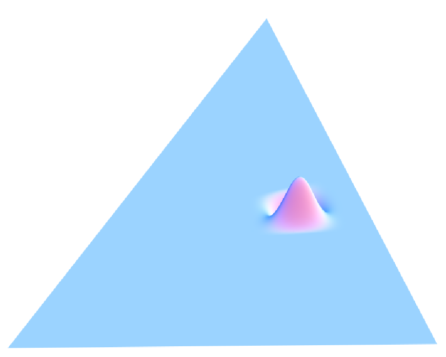
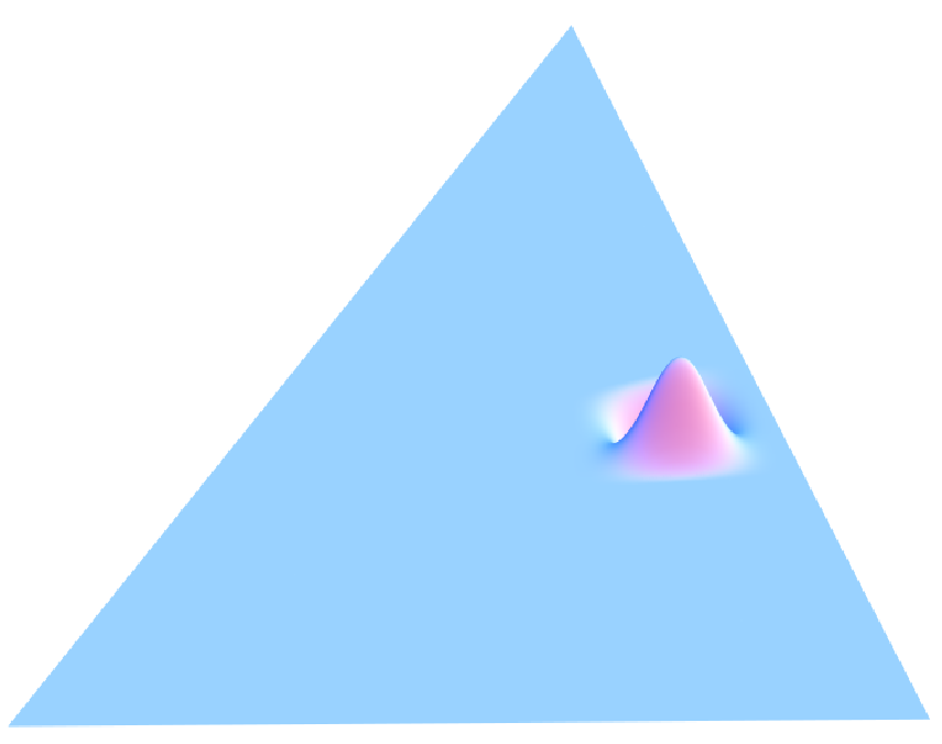
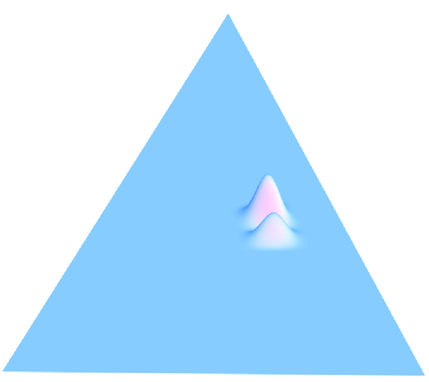
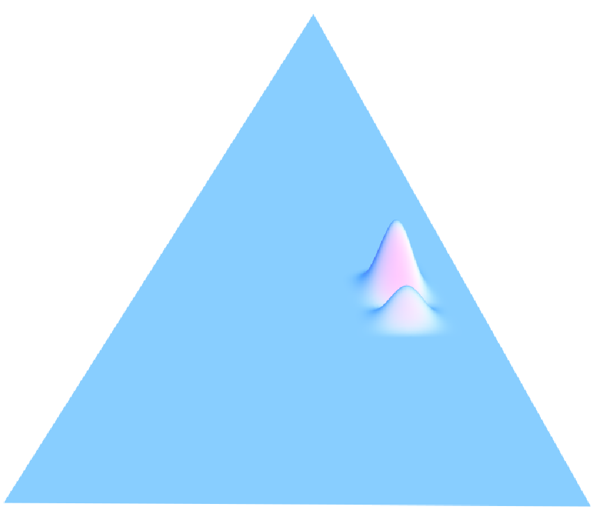
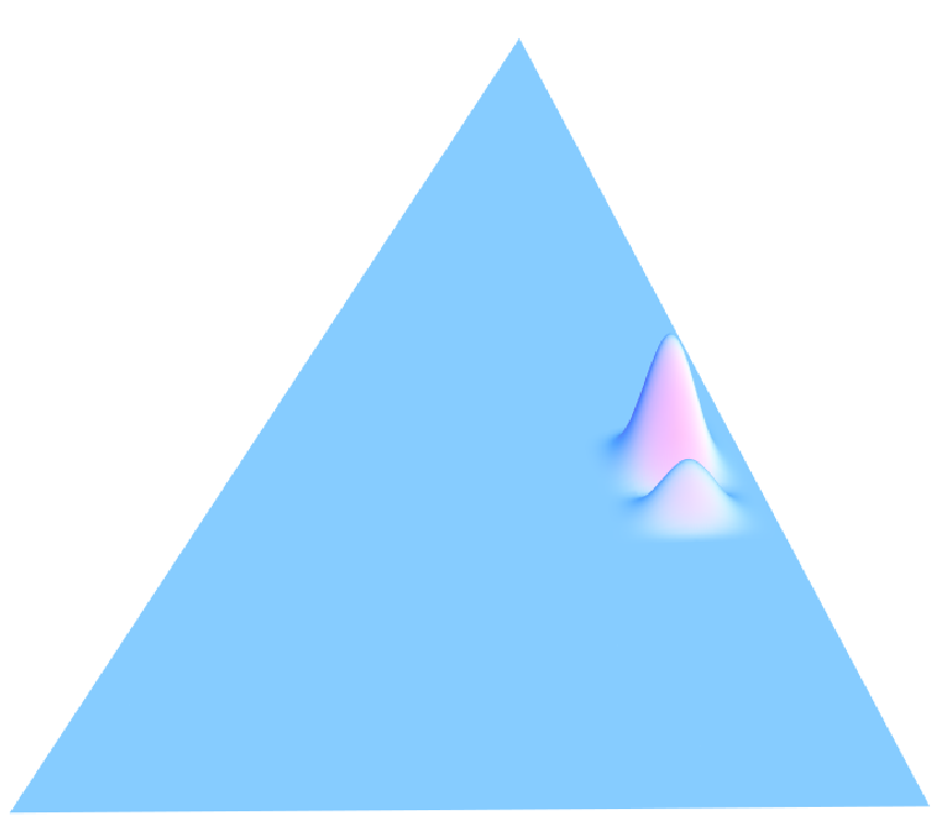
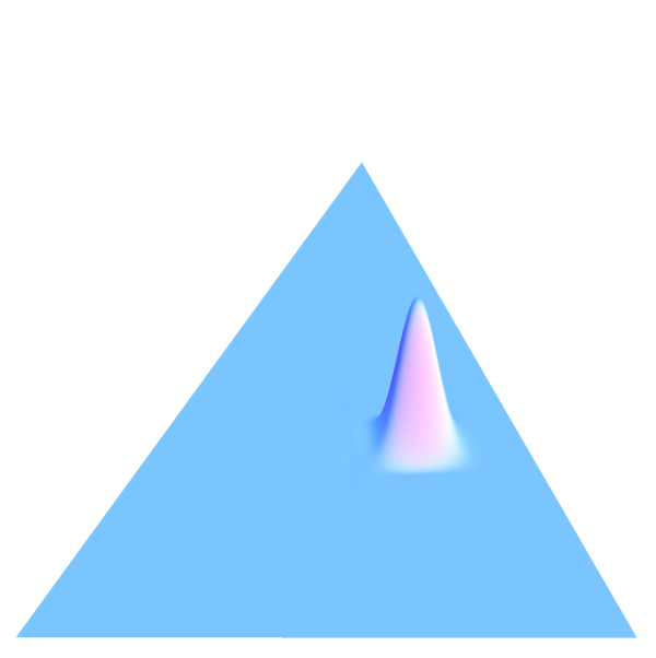
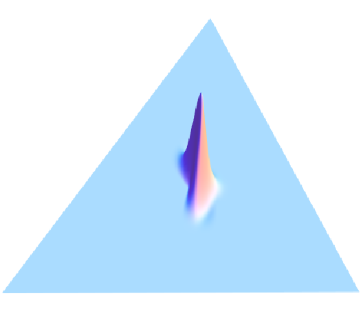
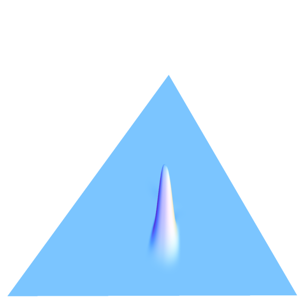
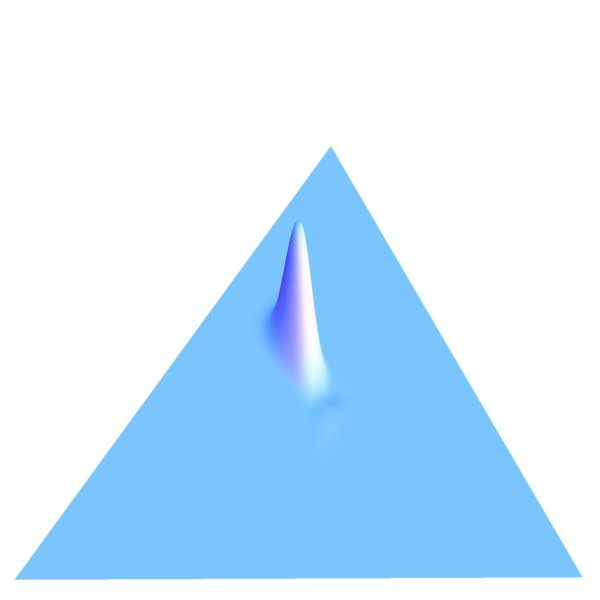
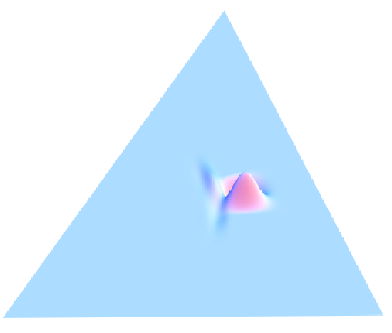
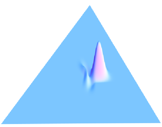
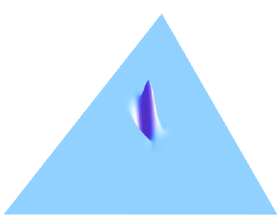
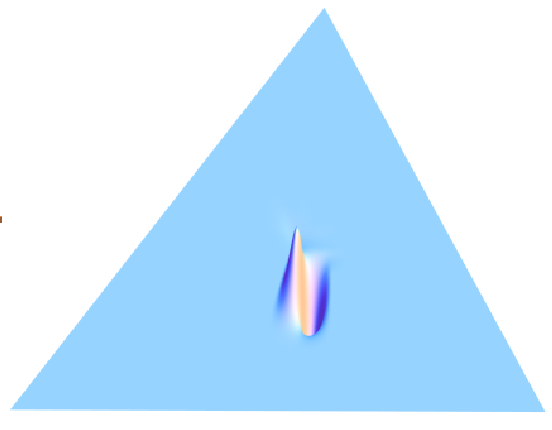
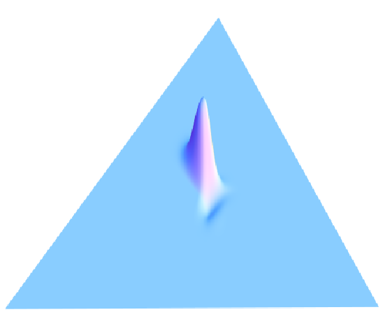
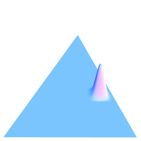
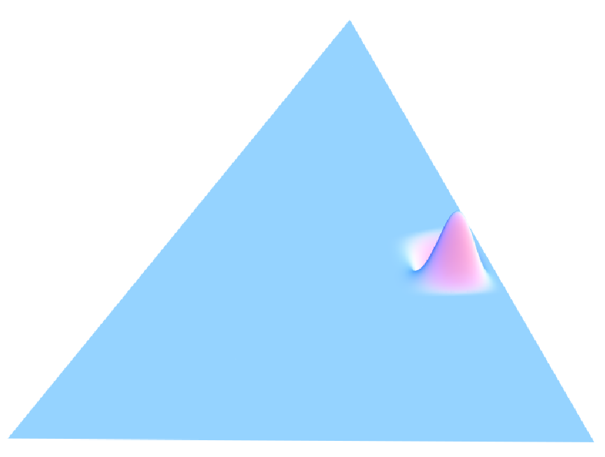
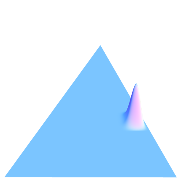
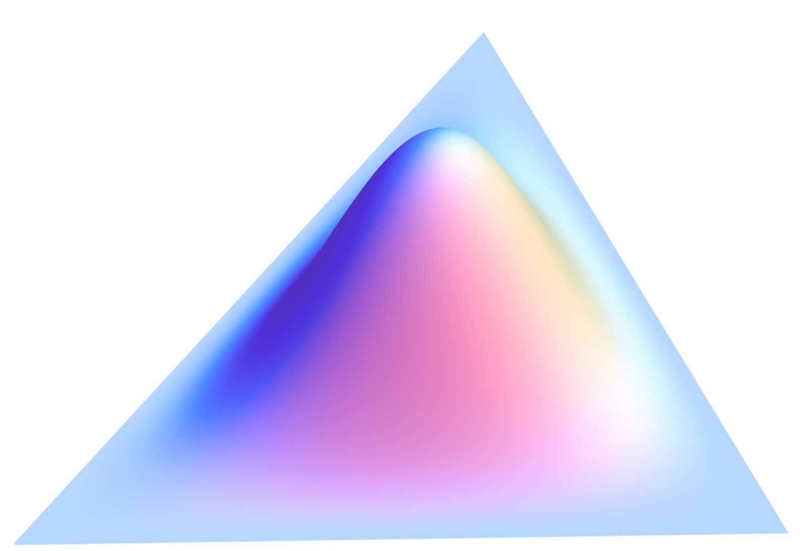
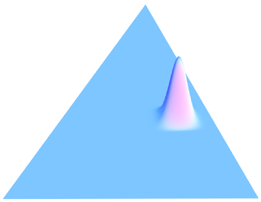
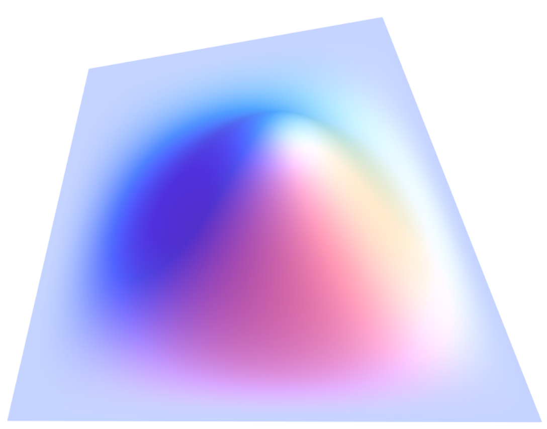
for s,ℓ=1,2,3s,\ell=1,2,3 and ρ=2,3,4\rho=2,3,4. Furthermore, the functions of the edge space 𝒲0​h;Γ(1)\mathcal{W}_{0h;\Gamma^{(1)}} and the functions of the vertex spaces 𝒲0​h;𝒗(1)\mathcal{W}_{0h;\boldsymbol{v}^{(1)}} and 𝒲0​h;𝒗(2)\mathcal{W}_{0h;\boldsymbol{v}^{(2)}} are shown in Fig. 5 and Fig. 6, respectively. Recall that the functions of the edge spaces are determined by the explicit representation (12), and that the functions of the vertex spaces are defined via appropriate bases of the null spaces of the corresponding homogeneous linear systems (22), which are computed by means of the minimal determining set algorithm [23, Section 6.1].
Refer to caption Refer to caption Refer to caption
ϕΓ(1);0,5\phi_{\Gamma^{(1)};0,5} ϕΓ(1);1,4\phi_{\Gamma^{(1)};1,4} ϕΓ(1);1,5\phi_{\Gamma^{(1)};1,5}
Refer to caption Refer to caption Refer to caption
ϕΓ(1);2,3\phi_{\Gamma^{(1)};2,3} ϕΓ(1);2,4\phi_{\Gamma^{(1)};2,4} ϕΓ(1);2,5\phi_{\Gamma^{(1)};2,5}
Figure 5: Graphs of the functions of the edge space 𝒲0​h;Γ(1)\mathcal{W}_{0h;\Gamma^{(1)}} for p=5p=5, r=2r=2 and h=16h=\frac{1}{6} (cf. Example 1).
Refer to caption Refer to caption Refer to caption Refer to caption
ϕ𝒗(1);1\phi_{\boldsymbol{v}^{(1)};1} ϕ𝒗(1);2\phi_{\boldsymbol{v}^{(1)};2} ϕ𝒗(1);3\phi_{\boldsymbol{v}^{(1)};3} ϕ𝒗(1);4\phi_{\boldsymbol{v}^{(1)};4}
Refer to caption Refer to caption Refer to caption Refer to caption
ϕ𝒗(1);5\phi_{\boldsymbol{v}^{(1)};5} ϕ𝒗(1);6\phi_{\boldsymbol{v}^{(1)};6} ϕ𝒗(1);7\phi_{\boldsymbol{v}^{(1)};7} ϕ𝒗(1);8\phi_{\boldsymbol{v}^{(1)};8}
Refer to caption Refer to caption Refer to caption Refer to caption
ϕ𝒗(1);9\phi_{\boldsymbol{v}^{(1)};9} ϕ𝒗(1);10\phi_{\boldsymbol{v}^{(1)};10} ϕ𝒗(1);11\phi_{\boldsymbol{v}^{(1)};11} ϕ𝒗(1);12\phi_{\boldsymbol{v}^{(1)};12}
Refer to caption Refer to caption Refer to caption Refer to caption
ϕ𝒗(1);13\phi_{\boldsymbol{v}^{(1)};13} ϕ𝒗(1);14\phi_{\boldsymbol{v}^{(1)};14} ϕ𝒗(1);15\phi_{\boldsymbol{v}^{(1)};15} ϕ𝒗(1);16\phi_{\boldsymbol{v}^{(1)};16}
Refer to caption Refer to caption Refer to caption
ϕ𝒗(2);1\phi_{\boldsymbol{v}^{(2)};1} ϕ𝒗(2);2\phi_{\boldsymbol{v}^{(2)};2} ϕ𝒗(2);3\phi_{\boldsymbol{v}^{(2)};3}
Figure 6: Graphs of the functions of the vertex spaces 𝒲0​h;𝒗(1)\mathcal{W}_{0h;\boldsymbol{v}^{(1)}} and 𝒲0​h;𝒗(2)\mathcal{W}_{0h;\boldsymbol{v}^{(2)}} for p=5p=5, r=2r=2 and h=16h=\frac{1}{6} (cf. Example 1).
Remark 5.

For the sake of simplicity we restricted ourselves to the case of bilinearly parameterized multi-patch domains. The construction of the space 𝒲0​h\mathcal{W}_{0h} and of its basis should be extendable in a straightforward way to the class of bilinear-like geometries [24]. However, the construction and the study of bilinear-like geometries themselves are limited to the case of two-patch domains [24] so far. But an extension to the case of multi-patch domains is of vital interest for the future research.

5 Solving the triharmonic equation – Examples

We present several examples to demonstrate the potential of our approach for solving the triharmonic equation over bilinear multi-patch domains.

Example 2.

We consider the three bilinearly parameterized multi-patch domains given in Figure 7 (first row), which possess extraordinary vertices of valency 33, 55 or 66 and describe a triangular, pentagonal and hexagonal domain, respectively. For all three domains (a)-(c), we construct nested isogeometric spline spaces 𝒲0​h\mathcal{W}_{0h} of degree p=5p=5 and regularity r=2r=2 for the mesh-sizes h=1k+1h=\frac{1}{k+1}, k∈{3,7,15,31}k\in\{3,7,15,31\}. Note that for the case of h=14h=\frac{1}{4}, the construction of the space 𝒲0​h\mathcal{W}_{0h} has to be slightly modified. More precisely, the vertex subspace 𝒲0​h;𝒗(ρ)\mathcal{W}_{0h;\boldsymbol{v}^{(\rho)}} is constructed without the use of the functions ϕΓ(ℓ);0,4\phi_{\Gamma^{(\ell)};0,4}. Instead, these functions are added to the corresponding edge subspaces 𝒲0​h;Γ(ℓ)\mathcal{W}_{0h;\Gamma^{(\ell)}} after subtracting suitable linear combinations of functions ϕΓ(ℓ);i,j\phi_{\Gamma^{(\ell)};i,j}, 0≤i≤20\leq i\leq 2, 0≤j≤min⁡(4−i,3)0\leq j\leq\min(4-i,3) to obtain functions ϕ^Γ(ℓ);0,4\widehat{\phi}_{\Gamma^{(\ell)};0,4} which have vanishing values, gradients and Hessians on ∂(Ω(ℓ−1)∪Ω(ℓ))\partial(\Omega^{(\ell-1)}\cup\Omega^{(\ell)}).

We solve the triharmonic equation (1) with the homogeneous boundary conditions (2) over the domains (a)-(c) for right side functions ff obtained by the exact solutions

ua​(𝒙)=(120​x2​(12​x113−x2)​(120−12​x17−x2))3,\footnotesize u_{a}(\boldsymbol{x})=\left(\frac{1}{20}x_{2}(\frac{12x_{1}}{13}-x_{2})(\frac{120-12x_{1}}{7}-x_{2})\right)^{3},
ub​(𝒙)=(120000​(121+8​x115−x2)​(7​x12+x2)​x2​(523−13​x16+x2)​(312−9​x111−x2))3\footnotesize u_{b}(\boldsymbol{x})=\left(\frac{1}{20000}(\frac{121+8x_{1}}{15}-x_{2})(\frac{7x_{1}}{2}+x_{2})x_{2}(\frac{52}{3}-\frac{13x_{1}}{6}+x_{2})(\frac{31}{2}-\frac{9x_{1}}{11}-x_{2})\right)^{3}

and

uc​(𝒙)=(1200000​(55−5​x12−x2)​(1799160−7​x164−x2)​(652+78​x161−x2)​(−18​x111−x2)​x2​(5​x13−10−x2))3,\footnotesize u_{c}(\boldsymbol{x})=\left(\frac{1}{200000}(\frac{55-5x_{1}}{2}-x_{2})(\frac{1799}{160}-\frac{7x_{1}}{64}-x_{2})(\frac{652+78x_{1}}{61}-x_{2})(-\frac{18x_{1}}{11}-x_{2})x_{2}(\frac{5x_{1}}{3}-10-x_{2})\right)^{3},

see Fig. 7 (second row). The resulting relative HiH^{i}-errors, i=0,1,2,3i=0,1,2,3, are visualized in Fig. 7 (third row) and indicate convergence rates of order 𝒪⁡(h6−i)\mathcal{O}(h^{6-i}) in the corresponding norms. 22 2 Note that for the spaces 𝒲0​h\mathcal{W}_{0h} the norms ||⋅||H3​(Ω)||\cdot||_{H^{3}(\Omega)} and ‖∇△​(⋅)‖L2​(Ω)||\nabla\triangle(\cdot)||_{L^{2}(\Omega)} are equivalent. Furthermore, Fig. 7 (fourth row) shows the resulting condition numbers κ\kappa of the stiffness matrices SS by using diagonally scaling (cf. [7]) and by employing no preconditioner. In case of the non-preconditioned stiffness matrices, the errors are slightly higher, but for both cases the estimated growth rates are of order 𝒪⁡(h−6)\mathcal{O}(h^{-6}), which demonstrate that the constructed basis functions are well-conditioned.
(a) (b) (c)
Computational domains Ω\Omega
Refer to caption Refer to caption Refer to caption
Exact solutions
Relative HiH^{i}-errors, i=0,…,3i=0,\ldots,3
Condition numbers κ\kappa of the preconditioned and non-preconditioned stiffness matrices SS
Figure 7: Solving the triharmonic equation over different multi-patch domains Ω\Omega (cf. Example 2).
Example 3.

We consider the bilinearly parameterized five-patch domain with four extraordinary vertices of valency 33, which is visualized in Fig. 8 (first row). For the mesh-sizes h=1k+1h=\frac{1}{k+1}, k∈{3,7,15,31}k\in\{3,7,15,31\}, nested isogeometric spline spaces 𝒲0​h\mathcal{W}_{0h} of degree p=5,6p=5,6 and regularity r=2r=2 (for p=5,6p=5,6) and r=3r=3 (for p=6p=6) are generated. As in Example 2, the construction of the space 𝒲0​h\mathcal{W}_{0h} has to be slightly changed for the case p=5p=5, r=2r=2 and h=14h=\frac{1}{4}. The resulting spaces are used to solve the triharmonic equation (1) with the homogeneous boundary conditions (2). We use for testing the right side function ff which is obtained by the exact solution

u⁡(𝒙)=(120000​x2​(4058−27​x18−x2)​(42538+4​x119−x2)​(23​x13−x2))3,u(\boldsymbol{x})=(\frac{1}{20000}x_{2}(\frac{405}{8}-\frac{27x_{1}}{8}-x_{2})(\frac{425}{38}+\frac{4x_{1}}{19}-x_{2})(\frac{23x_{1}}{3}-x_{2}))^{3},

see Fig. 8 (first row). The resulting relative HiH^{i}-errors are of order 𝒪⁡(hp+1−i)\mathcal{O}(h^{p+1-i}), and the estimated growth rates of the diagonally scaled stiffness matrices SS are of order 𝒪⁡(h−6)\mathcal{O}(h^{-6}). As in Example 2, we also present the condition numbers of the non-preconditioned stiffness matrices SS, see Fig. 8, which are again slightly higher than for the preconditioned case (i.e. using diagonal scaling) but still seems to grow of order 𝒪⁡(h−6)\mathcal{O}(h^{-6}). This indicates again that the constructed basis functions are well-conditioned.

Refer to caption
Computational domain Exact solution
Relative HiH^{i}-errors, i=0,…,3i=0,\ldots,3
Condition numbers κ\kappa of preconditioned and non-preconditioned stiffness matrices SS
Figure 8: Solving the triharmonic equation over the given multi-patch domain Ω\Omega (cf. Example 3).

6 Conclusion

We described a method for solving the triharmonic equation over bilinearly parameterized planar multi-patch domains. The presented approach is based on the concept of IGA and uses as discretization space 𝒲0​h\mathcal{W}_{0h} a space of globally C2C^{2}-smooth isogeometric functions. The discretization space 𝒲0​h\mathcal{W}_{0h} is the span of three different types of basis functions called patch, edge and vertex functions. All of these functions possess a simple representation with small local supports, can be uniformly generated for all possible multi-patch configurations, and numerical examples indicate that they are well-conditioned. The numerical results obtained by solving the triharmonic equation over different bilinear multi-patch domains using hh-refinement demonstrate the potential of our approach.

The paper leaves several open questions which are worth to study. A first possible topic for future research could be the study of a priori error estimates for the triharmonic equation over multi-patch domains under hh-refinement (similar to the ones in [44] for single patch domains), and the theoretical investigation of the approximation properties of the discretization space 𝒲0​h\mathcal{W}_{0h}. Another topic could be the detailed study of the dimension of the space 𝒲0​h\mathcal{W}_{0h} to get an explicit dimension formula. In [22], the case of the entire C2C^{2}-smooth space 𝒱h\mathcal{V}_{h} was investigated, and the obtained formula there provides an upper bound for the dimension of 𝒲0​h\mathcal{W}_{0h}. Like in [22] for the case of 𝒱h\mathcal{V}_{h}, the dimension of the space 𝒲0​h\mathcal{W}_{0h} is just the sum of the dimensions of the single subspaces (i.e. patch, edge and vertex subspaces). While the numbers of basis functions for the patch subspaces 𝒲0​h;Ω(ℓ)\mathcal{W}_{0h;\Omega^{(\ell)}} and for the edge subspaces 𝒲0​h;Γ(s)\mathcal{W}_{0h;\Gamma^{(s)}} are explicitly given, the computation of the numbers of basis functions for the vertex subspaces 𝒲0​h;𝒗(ρ)\mathcal{W}_{0h;\boldsymbol{v}^{(\rho)}} still deserves further investigation.

Moreover, one could consider further 66-th order PDEs for which the use of the discretization space 𝒲0​h\mathcal{W}_{0h} could be suitable, since these problems require functions of C2C^{2}-smoothness. Possible examples are the Kirchhoff plate model based on the Mindlin’s gradient elasticity theory [38], the Phase-field crystal equation [1, 14] and the gradient-enhanced continuum damage model [48]. The extension of our approach to more general multi-patch domains, such as e.g., bilinear-like planar domains, shells or volumetric domains could be considered, too.

Acknowledgment

The authors wish to thank the anonymous reviewers for their comments that helped to improve the paper. V. Vitrih was partially supported by the Slovenian Research Agency (research program P1-0285). This support is gratefully acknowledged.

Appendix A Proof of Proposition 1

The proof will be mainly based on the concept of blossoming. Let q∈𝒮hp,r​([0,1])q\in\mathcal{S}_{h}^{p,r}([0,1]), and let t0p,r,t1p,r,…,t2​p+1+k⁡(p−r)p,rt_{0}^{p,r},t_{1}^{p,r},\ldots,t_{2p+1+k(p-r)}^{p,r} be the corresponding knots of the spline space 𝒮hp,r​([0,1])\mathcal{S}_{h}^{p,r}([0,1]). Then there exists a unique function 𝒬p,r:ℝp→ℝ\mathcal{Q}^{p,r}:{\color[rgb]{0,0,0}\mathbb{R}^{p}\to\mathbb{R}}, called the blossom of qq, which is symmetric, multi-affine and fulfill 𝒬p,r​(ξ,ξ,…,ξ)=q⁡(ξ)\mathcal{Q}^{p,r}(\xi,\xi,\ldots,\xi)=q(\xi). These properties imply that the control points of qq can be written as

dι=𝒬p,r(tι+1p,r,tι+2p,r,…,tι+pp,r),ι=0,1,…,p+k(p−r).d_{\iota}=\mathcal{Q}^{p,r}(t_{\iota+1}^{p,r},t_{\iota+2}^{p,r},\ldots,t_{\iota+p}^{p,r}),\quad\iota=0,1,\ldots,p+k(p-r).

Blossoming is a simple approach, which can be used amongst others to perform knot insertion for a spline function or to multiply two spline functions. For more details about the concept of blossoming we refer to e.g. [12, 40, 41].

The following two lemmas will be needed.

Lemma 5.

Let Njp,r+1​(ξ)=∑ι=0p+k⁡(p−r)d~ι​Nιp,r​(ξ)N_{j}^{p,r+1}(\xi)=\sum_{\iota=0}^{p+k(p-r)}\widetilde{d}_{\iota}N_{\iota}^{p,r}(\xi). Then d~ι=0\widetilde{d}_{\iota}=0 for ι<j.\iota<j.

proof 2.

Let dιd_{\iota} be control points of Njp,r+1∈𝒮hp,r+1​([0,1])N_{j}^{p,r+1}\in\mathcal{S}_{h}^{p,r+1}([0,1]), i.e., dι=δj,ιd_{\iota}=\delta_{j,\iota}. Moreover let d~ι\widetilde{d}_{\iota} denote control points of Njp,r+1N_{j}^{p,r+1} represented in the space 𝒮hp,r​([0,1])\mathcal{S}_{h}^{p,r}([0,1]). Then (see e.g. [12])

d~ι=𝒬p,r+1​(tι+1p,r,…,tι+pp,r).\widetilde{d}_{\iota}=\mathcal{Q}^{p,r+1}(t_{\iota+1}^{p,r},\ldots,t_{\iota+p}^{p,r}).

Since

dι=𝒬p,r+1​(tι+1p,r+1,…,tι+pp,r+1)andtι+pp,r+1≥tι+pp,r,{d}_{\iota}=\mathcal{Q}^{p,r+1}(t_{\iota+1}^{p,r+1},\ldots,t_{\iota+p}^{p,r+1})\quad{\rm and}\quad t_{\iota+p}^{p,r+1}\geq t_{\iota+p}^{p,r},

it follows that d~ι=∑m≤ιcm​dm\widetilde{d}_{\iota}=\sum_{m\leq\iota}c_{m}d_{m}, cm∈ℝc_{m}\in\mathbb{R}, which implies d~ι=0\widetilde{d}_{\iota}=0 for ι<j\iota<j. ∎

Lemma 6.

Let (ω0​(1−ξ)+ω1​ξ)​Njp−1,r​(ξ)=∑ι=0p+k⁡(p−r)d^ι​Nιp,r​(ξ)(\omega_{0}(1-\xi)+\omega_{1}\xi)\,N_{j}^{p-1,r}(\xi)=\sum_{\iota=0}^{p+k(p-r)}\widehat{d}_{\iota}N_{\iota}^{p,r}(\xi). Then d^ι=0\widehat{d}_{\iota}=0 for ι<j.\iota<j.

proof 3.

Let dιd_{\iota} denote control points of Njp−1,r∈𝒮hp−1,r​([0,1])N_{j}^{p-1,r}\in\mathcal{S}_{h}^{p-1,r}([0,1]), i.e., dι=δj,ιd_{\iota}=\delta_{j,\iota}, and let 𝒬p−1,r\mathcal{Q}^{p-1,r} denote its blossom. Moreover let d^ι\widehat{d}_{\iota} denote the control points of (ω0​(1−ξ)+ω1​ξ)​Njp−1,r​(ξ)∈𝒮hp,r​([0,1])(\omega_{0}(1-\xi)+\omega_{1}\xi)\,N_{j}^{p-1,r}(\xi)\in\mathcal{S}_{h}^{p,r}([0,1]). Then (see e.g. [12])

d^ι=1p​∑m=1p𝒬p−1,r​(tι+1p,r,…,tι+m−1p,r,tι+m+1p,r,…,tι+pp,r)​(ω0​(1−tι+mp,r)+ω1​tι+mp,r).\widehat{d}_{\iota}=\frac{1}{p}\sum_{m=1}^{p}\mathcal{Q}^{p-1,r}(t_{\iota+1}^{p,r},\ldots,t_{\iota+m-1}^{p,r},t_{\iota+m+1}^{p,r},\ldots,t_{\iota+p}^{p,r})\left(\omega_{0}(1-t_{\iota+m}^{p,r})+\omega_{1}t_{\iota+m}^{p,r}\right).

We have to prove that d^ι=∑n≤ιcn​dn\widehat{d}_{\iota}=\sum_{n\leq\iota}c_{n}d_{n}, cn∈ℝc_{n}\in\mathbb{R}. Since dι=𝒬p−1,r​(tι+1p−1,r,…,tι+pp−1,r)d_{\iota}=\mathcal{Q}^{p-1,r}(t_{\iota+1}^{p-1,r},\ldots,t_{\iota+p}^{p-1,r}) and tι+pp,r≤tι+pp−1,rt_{\iota+p}^{p,r}\leq t_{\iota+p}^{p-1,r}, it follows that 𝒬p−1,r​(tι+1p,r,…,tι+m−1p,r,tι+m+1p,r,…,tι+pp,r)\mathcal{Q}^{p-1,r}(t_{\iota+1}^{p,r},\ldots,t_{\iota+m-1}^{p,r},t_{\iota+m+1}^{p,r},\ldots,t_{\iota+p}^{p,r}) does not involve dnd_{n}, n>ιn>\iota. Therefore d^ι\widehat{d}_{\iota} is independent of dnd_{n}, n>ιn>\iota, implying d^ι=0\widehat{d}_{\iota}=0 for ι<j\iota<j. ∎

Proof of Proposition 1: Recall (12). We first observe that the first summation in (13) follows directly from (10). It remains to prove that the only nonzero coefficients dΓ(s);m,n(τ)d_{\Gamma^{(s)};m,n}^{(\tau)} might be the ones with n≥max⁡(0,i+j−m)n\geq\max(0,i+j-m) and n≤min⁡(d−1,d−ni+j−i+m)n\leq\min(d-1,d-n_{i}+j-i+m).

The lower bound follows immediately by using

(Njp,r​(ξ))′=∑ι=j−1jdι​Nιp−1,r−1​(ξ),(Njp,r​(ξ))′′=∑ι=j−2jcι​Nιp−2,r−2​(ξ),\left(N_{j}^{p,r}(\xi)\right)^{\prime}=\sum_{\iota=j-1}^{j}d_{\iota}\,N_{\iota}^{p-1,r-1}(\xi),\quad\left(N_{j}^{p,r}(\xi)\right)^{\prime\prime}=\sum_{\iota=j-2}^{j}c_{\iota}\,N_{\iota}^{p-2,r-2}(\xi),

and by Lemma 5 and Lemma 6. The upper bound can be shown by first considering the function

g^Γ(s);i,j(τ)​(ξ1(τ),ξ2(τ))=gΓ(s);i,ni−1−j(τ)​(ξ1(τ),1−ξ2(τ)),\widehat{g}^{(\tau)}_{\Gamma^{(s)};i,j}(\xi_{1}^{(\tau)},\xi_{2}^{(\tau)})=g^{(\tau)}_{\Gamma^{(s)};i,n_{i}-1-j}(\xi_{1}^{(\tau)},1-\xi_{2}^{(\tau)}),

which possesses again the lower bound n≥max⁡(0,i+j−m)n\geq\max(0,i+j-m) for possible nonzero coefficients d^Γ(s);m,n(τ)\widehat{d}_{\Gamma^{(s)};m,n}^{(\tau)}. This directly implies the upper bound n≤min⁡(d−1,d−ni+j−i+m)n\leq\min(d-1,d-n_{i}+j-i+m) for possible nonzero coefficients dΓ(s);m,n(τ)d_{\Gamma^{(s)};m,n}^{(\tau)} of the function gΓ(s);i,j(τ)g^{(\tau)}_{\Gamma^{(s)};i,j}. ∎

References

  • [1] A. Bartezzaghi, L. Dedè, and A. Quarteroni. Isogeometric analysis of high order partial differential equations on surfaces. Comput. Methods Appl. Mech. Engrg., 295:446 – 469, 2015.
  • [2] L. Beirão da Veiga, A. Buffa, G. Sangalli, and R. Vázquez. Mathematical analysis of variational isogeometric methods. Acta Numerica, 23:157–287, 5 2014.
  • [3] L. Beirão Da Veiga, T. J. R. Hughes, J. Kiendl, C. Lovadina, J. Niiranen, A. Reali, and H. Speleers. A locking-free model for Reissner-Mindlin plates: analysis and isogeometric implementation via NURBS and triangular NURPS. Math. Models Methods Appl. Sci., 25(8):1519–1551, 2015.
  • [4] D. J. Benson, Y. Bazilevs, M.-C. Hsu, and T. J.R. Hughes. A large deformation, rotation-free, isogeometric shell. Comput. Methods Appl. Mech. Engrg., 200(13):1367–1378, 2011.
  • [5] M. Bercovier and T. Matskewich. Smooth Bézier Surfaces over Unstructured Quadrilateral Meshes. Lecture Notes of the Unione Matematica Italiana, Springer, 2017.
  • [6] A. Blidia, B. Mourrain, and N. Villamizar. G1-smooth splines on quad meshes with 4-split macro-patch elements. Comput. Aided Geom. Des., 52–-53:106 – 125, 2017.
  • [7] A. M. Bruaset. A survey of preconditioned iterative methods, volume 328 of Pitman Research Notes in Mathematics Series. Longman Scientific & Technical, Harlow, 1995.
  • [8] A. Collin, G. Sangalli, and T. Takacs. Analysis-suitable G1 multi-patch parametrizations for C1 isogeometric spaces. Computer Aided Geometric Design, 47:93 – 113, 2016.
  • [9] J. A. Cottrell, T.J.R. Hughes, and Y. Bazilevs. Isogeometric Analysis: Toward Integration of CAD and FEA. John Wiley & Sons, Chichester, England, 2009.
  • [10] O. Davydov and W. P. Yeo. Refinable C2C^{2} piecewise quintic polynomials on Powell-Sabin-12 triangulations. J. Comput. Appl. Math., 240:62–73, 2013.
  • [11] P. Fischer, M. Klassen, J. Mergheim, P. Steinmann, and R. Müller. Isogeometric analysis of 2D gradient elasticity. Comput. Mech., 47(3):325–334, 2011.
  • [12] R. Goldman. Pyramid algorithms : a dynamic programming approach to curves and surfaces for geometric modeling. Morgan Kaufmann, San Francisco (Calif.), 2003.
  • [13] H. Gómez, V. M Calo, Y. Bazilevs, and T. J.R. Hughes. Isogeometric analysis of the Cahn–Hilliard phase-field model. Comput. Methods Appl. Mech. Engrg., 197(49):4333–4352, 2008.
  • [14] H. Gomez and X. Nogueira. An unconditionally energy-stable method for the phase field crystal equation. Computer Methods in Applied Mechanics and Engineering, 249 – 252:52 – 61, 2012.
  • [15] D. Groisser and J. Peters. Matched Gk-constructions always yield Ck-continuous isogeometric elements. Computer Aided Geometric Design, 34:67 – 72, 2015.
  • [16] J. Grošelj. A normalized representation of super splines of arbitrary degree on Powell-Sabin triangulations. BIT Numerical Mathematics, 56(4):1257–1280, 2016.
  • [17] J. Hoschek and D. Lasser. Fundamentals of computer aided geometric design. A K Peters Ltd., Wellesley, MA, 1993.
  • [18] T. J. R. Hughes, J. A. Cottrell, and Y. Bazilevs. Isogeometric analysis: CAD, finite elements, NURBS, exact geometry and mesh refinement. Comput. Methods Appl. Mech. Engrg., 194(39-41):4135–4195, 2005.
  • [19] M. Kapl, F. Buchegger, M. Bercovier, and B. Jüttler. Isogeometric analysis with geometrically continuous functions on planar multi-patch geometries. Comput. Methods Appl. Mech. Engrg., 316:209 – 234, 2017.
  • [20] M. Kapl, G. Sangalli, and T. Takacs. Analysis-suitable C1{C}^{1} multi-patch isogeometric spaces: basis and dual basis. Technical Report 1711.05161, arXiv.org, 2017.
  • [21] M. Kapl, G. Sangalli, and T. Takacs. Dimension and basis construction for analysis-suitable G1 two-patch parameterizations. Computer Aided Geometric Design, 52–53:75 – 89, 2017.
  • [22] M. Kapl and V. Vitrih. Space of C2-smooth geometrically continuous isogeometric functions on planar multi-patch geometries: Dimension and numerical experiments. Comput. Math. Appl., 73(10):2319––2338, 2017.
  • [23] M. Kapl and V. Vitrih. Space of C2-smooth geometrically continuous isogeometric functions on two-patch geometries. Comput. Math. Appl., 73(1):37 – 59, 2017.
  • [24] M. Kapl and V. Vitrih. Dimension and basis construction for C2{C}^{2}-smooth isogeometric spline spaces over bilinear-like G2{G}^{2} two-patch parameterizations. Journal of Computational and Applied Mathematics, 335:289–311, 2018.
  • [25] M. Kapl, V. Vitrih, B. Jüttler, and K. Birner. Isogeometric analysis with geometrically continuous functions on two-patch geometries. Comput. Math. Appl., 70(7):1518 – 1538, 2015.
  • [26] K. Karčiauskas, T. Nguyen, and J. Peters. Generalizing bicubic splines for modeling and IGA with irregular layout. Computer-Aided Design, 70:23 – 35, 2016.
  • [27] S. Khakalo and J. Niiranen. Isogeometric analysis of higher-order gradient elasticity by user elements of a commercial finite element software. Comput.-Aided Des., 82:154–169, 2017.
  • [28] J. Kiendl, Y. Bazilevs, M.-C. Hsu, R. Wüchner, and K.-U. Bletzinger. The bending strip method for isogeometric analysis of Kirchhoff-Love shell structures comprised of multiple patches. Comput. Methods Appl. Mech. Engrg., 199(35):2403–2416, 2010.
  • [29] J. Kiendl, K.-U. Bletzinger, J. Linhard, and R. Wüchner. Isogeometric shell analysis with Kirchhoff-Love elements. Comput. Methods Appl. Mech. Engrg., 198(49):3902–3914, 2009.
  • [30] J. Kiendl, M.-Ch. Hsu, M. C. H. Wu, and A. Reali. Isogeometric Kirchhoff–Love shell formulations for general hyperelastic materials. Comput. Methods Appl. Mech. Engrg., 291:280 – 303, 2015.
  • [31] M.-J. Lai and L. L. Schumaker. Spline functions on triangulations, volume 110 of Encyclopedia of Mathematics and its Applications. Cambridge University Press, Cambridge, 2007.
  • [32] J. Liu, L. Dedè, J. A. John A Evans, M. J. Borden, and T. J. R. Hughes. Isogeometric analysis of the advective Cahn–Hilliard equation: Spinodal decomposition under shear flow. Journal of Computational Physics, 242:321 – 350, 2013.
  • [33] T. Lyche and G. Muntingh. A Hermite interpolatory subdivision scheme for C2C^{2}-quintics on the Powell-Sabin 12-split. Comput. Aided Geom. Design, 31(7-8):464–474, 2014.
  • [34] B. Mourrain, R. Vidunas, and N. Villamizar. Dimension and bases for geometrically continuous splines on surfaces of arbitrary topology. Computer Aided Geometric Design, 45:108 – 133, 2016.
  • [35] T. Nguyen and J. Peters. Refinable C1{C}^{1} spline elements for irregular quad layout. Computer Aided Geometric Design, 43:123 – 130, 2016.
  • [36] N. Nguyen-Thanh, K. Zhou, X. Zhuang, P. Areias, H. Nguyen-Xuan, Y. Bazilevs, and T. Rabczuk. Isogeometric analysis of large-deformation thin shells using RHT-splines for multiple-patch coupling. Computer Methods in Applied Mechanics and Engineering, 316:1157 – 1178, 2017.
  • [37] J. Niiranen, S. Khakalo, V. Balobanov, and A. H. Niemi. Variational formulation and isogeometric analysis for fourth-order boundary value problems of gradient-elastic bar and plane strain/stress problems. Comput. Methods Appl. Mech. Engrg., 308:182–211, 2016.
  • [38] J. Niiranen, J. Kiendl, A. H. Niemi, and A. Reali. Isogeometric analysis for sixth-order boundary value problems of gradient-elastic Kirchhoff plates. Computer Methods in Applied Mechanics and Engineering, 316:328––348, 2017.
  • [39] J. Peters. Geometric continuity. In Handbook of computer aided geometric design, pages 193–227. North-Holland, Amsterdam, 2002.
  • [40] L. Ramshaw. Blossoms are polar forms. Comput. Aided Geom. Des., 6(4):323–358, 1989.
  • [41] H.-P. Seidel. An introduction to polar forms. IEEE Computer Graphics and Applications, 13(1):38–46, 1993.
  • [42] H. Speleers. Interpolation with quintic Powell-Sabin splines. Appl. Numer. Math., 62(5):620–635, 2012.
  • [43] H. Speleers. Construction of normalized B-splines for a family of smooth spline spaces over Powell-Sabin triangulations. Constr. Approx., 37(1):41–72, 2013.
  • [44] A. Tagliabue, L. Dedè, and A. Quarteroni. Isogeometric analysis and error estimates for high order partial differential equations in fluid dynamics. Computers & Fluids, 102:277 – 303, 2014.
  • [45] D. Toshniwal, H. Speleers, R. Hiemstra, and T. J. R. Hughes. Multi-degree smooth polar splines: A framework for geometric modeling and isogeometric analysis. Comput. Methods Appl. Mech. Engrg., 2016.
  • [46] D. Toshniwal, H. Speleers, and Hughes T. J. R. Analysis-suitable spline spaces of arbitrary degree on unstructured quadrilateral meshes. Technical Report 16, Institute for Computational Engineering and Sciences (ICES), 2017.
  • [47] D. Toshniwal, H. Speleers, and Hughes T. J. R. Smooth cubic spline spaces on unstructured quadrilateral meshes with particular emphasis on extraordinary points: Geometric design and isogeometric analysis considerations. Comput. Methods Appl. Mech. Engrg., 327:411–458, 2017.
  • [48] C. V. Verhoosel, M. A. Scott, T. J. R. Hughes, and R. de Borst. An isogeometric analysis approach to gradient damage models. Internat. J. Numer. Methods Engrg., 86(1):115–134, 2011.