Phase transition with trivial quantum criticality in anisotropic Weyl semimetal

Weakly interacting metals are perfectly described by the Fermi liquid (FL) theory [1, 2, 3]. Coulomb interaction plays a negligible role since it becomes short-ranged due to the static screening caused by the collective particle-hole excitations. The static screening factor serves as an infrared cutoff for the transferred energy/momentum, which suppresses forward scattering and guarantees the stability of FL state. When gapless fermions couple to certain gapless bosonic mode, Landau damping could be strong enough to yield a vanishing quasiparticle residue $Z_{f}$, which implies the breakdown of FL theory. A prominent example is the system of fermions coupled to a U(1) gauge boson [4, 5, 6, 7, 8, 9, 10]. The gauge boson is strictly gapless, rendered by local gauge invariance, and leads to non-FL behavior characterized by $Z_{f}=0$.

When a metal undergoes a continuous quantum phase transition, non-FL behavior and other intriguing physical properties can emerge [11, 12]. Near the quantum critical point (QCP), the quantum fluctuation of order parameter becomes critical as the correlation length $\xi$ diverges, and can be described by the dynamics of gapless bosonic mode [13, 14, 15]. The low-energy behavior of the quantum criticality is determined by the coupling between gapless fermionic and bosonic degrees of freedom. Such coupling has been studied extensively in various quantum critical systems, including ferromagnetic (FM) QCP [16, 17, 18], antiferromagnetic (AFM) QCP [19, 20, 21], and Ising-type nematic QCP [22, 23, 24, 25]. In these systems, the fermion-boson coupling can generate a finite anomalous dimension for fermion field and also leads to strong Landau damping of fermions. At finite temperature, the QCP becomes a finite quantum critical regime, as schematically shown in Fig. 1(a), which can be called a NFL regime due to the strong violation of FL description. A popular notion is that, the observed superconducting (SC) dome and NFL normal-state properties in many cuprate, heavy fermion, and iron-based superconductors arise from the quantum fluctuation of certain long-range order.

Nontrivial quantum criticality also occurs in several semimetal (SM) materials [26, 27, 28, 29, 30, 31, 32, 33, 34]. Recently, SC transition and the associated quantum criticality have attracted particular research interest. In most SMs, Cooper pairing occurs only when the net attraction is larger than certain critical value [35, 36, 37, 38, 39, 40, 41, 42, 43, 44, 45, 46, 47, 48, 49, 50, 51, 52, 53, 54]. It is argued that the Yukawa coupling between gapless Dirac/Weyl fermions and bosonic SC order parameter might dynamically generate an emergent space-time supersymmetry [55, 56, 57, 58, 59, 60, 61]. These QCPs display a series of unusual quantum critical behaviors.

In this paper, we study the quantum criticality of SM-SC transition in a 3D anisotropic Weyl semimetal (AWSM), where the fermion dispersion is linear in two momentum exponents and quadratical in the third one [62, 63, 64]. Such an AWSM state emerges naturally as one pair of Weyl points of a Weyl SM merge into one single band-touching point. In the parent Weyl SM, the Chern numbers of one pair of Weyl points are $\pm 1$. When two Weyl points with opposite Chern numbers merge, the resultant band-touching point has zero Chern number [62, 63, 64]. Thus, the AWSM state is topologically trivial. Superconductivity is induced when the strength of net attraction, denoted by $g$, is larger than $g_{c}$. At $g=g_{c}$, the quantum fluctuation of SC order parameter is gapless and couples to gapless Weyl fermions. According to previous research experience, one would naively expect to observe a series of unusual quantum critical phenomena at the QCP.

We present a renormalization group (RG) study of the coupling between the Weyl fermions and the SC quantum fluctuation. Interestingly, although the SC quantum fluctuation is critical, the Weyl fermions do not acquire a finite anomalous dimension in the low-energy regime and the quasiparticle residue remains finite, namely $Z_{f}\neq 0$. This indicates that the SC quantum fluctuation does not qualitatively modify the low-energy properties of the system, and that the fermions behave in nearly the same way as free fermion gas in the non-SC phase. A simple mean-field treatment should suffice to describe the transition. We thus obtain an example of quantum phase transition that is characterized by trivial critical phenomena. As illustrated by Fig. 1, a large NFL-like quantum critical regime exists between the disordered and ordered phases in many quantum critical systems. In contrast, there is not such a NFL regime in 3D AWSM, which is caused by the special anisotropy of fermion dispersion.

The rest of the paper is organized as follows. In Sec. II, we first make a mean-field analysis and determine the SC QCP by solving the gap equation. In Sec. III, we will go beyond the mean-field level and study the influence of the quantum critical fluctuation of SC order parameter by performing a RG analysis. The low-energy behavior of all the model parameters are obtained from the solutions of the self-consistent RG equations. We briefly summarize the results and also discuss the possible experimental probe of our prediction in Sec. IV. The details of mean-field calculation and RG calculation are presented in Appendix A and Appendix B, respectively.

The system under consideration is described by the Hamiltonian $H=H_{0}+H_{I}$, where

where the fermion field operator is defined as $\psi_{\mathbf{k}}^{{\dagger}}=(c_{\mathbf{k},\uparrow}^{{\dagger}},c_{\mathbf{k},\downarrow}^{{\dagger}})$ to implement the spinor structure and $\sigma_{1,2,3}$ are the standard Pauli matrices. The fermion dispersion [62, 63, 64] has the form $E_{f}=\pm\sqrt{c_{f}^{2}k_{\bot}^{2}+A^{2}k_{z}^{4}}$, where $k_{\perp}^{2}=k_{x}^{2}+k_{y}^{2}$, and $c_{f}$ and $A$ are two parameters introduced to characterize the energy dispersions within $x$-$y$ plane and along $z$-axis, respectively. Here, we consider one single specie of anisotropic Weyl fermions. The short-range pairing interaction is described by $H_{I}$, where the coupling constant $g>0$.

We first make a mean-field analysis to determine the SC QCP. The SC order parameter is defined as

At the mean-field level, we have

where the SC gap is supposed to be $s$-wave. According to the calculations presented in Appendix A, the zero-temperature gap equation is

It is easy to verify that a nonzero SC gap is opened only when the coupling $g$ exceeds the critical value

where $E_{D}$ is a cutoff.

At the SM-SC QCP, the SC order parameter vanishes, namely $\langle\psi_{\mathbf{k}}(i\sigma_{2})\psi_{\mathbf{-k}}\rangle=0$. But its quantum fluctuation cannot be simply neglected. We will carry out a RG analysis to examine whether or not its quantum fluctuation leads to significant effects on the low-energy behavior of anisotropic Weyl fermions.

The quantum critical system can be modeled by the following effective action

where the free action for Weyl fermions is given by

where $\mathcal{H}_{\psi}(\mathbf{k})=c_{f}k_{x}\sigma_{1}+c_{f}k_{y}\sigma_{2}+Ak^{2}_{z}\sigma_{3}$, the one for SC order parameter is

where $E_{\phi}(\mathbf{q})=\sqrt{c_{b\perp}^{2}\left(q_{x}^{2}+q_{y}^{2}\right)+c_{bz}^{2}q_{z}^{2}}$. Here, $c_{b\perp}$ is the boson velocity within the $x$-$y$ plane and $c_{bz}$ the one along $z$-direction. The boson mass $r$ serves as a tuning parameter: $r>0$ corresponds to SM phase ($g<g_{c}$) and $r<0$ to SC phase ($g>g_{c}$). In the following, we focus on the SM-SC QCP, corrsponding to $r=0$. The free fermion and boson propagators are

The self-coupling of the boson field takes the form

where for simplicity we define

The Yukawa-coupling between the gapless fermions and the critical boson is described by

where $h$ is the coupling constant.

The whole action contains six model parameters, namely $c_{f}$, $A$, $c_{b\bot}$, $c_{bz}$, $\lambda$, and $h$. These parameters all receive quantum corrections from the Yukawa coupling, and then become scale dependent. The low-energy critical behavior of the SC QCP can be analyzed based on the scale dependence of all these parameters. After carrying out lengthy calculations, with full details presented in Appendices B and C, we derive the following coupled RG equations:

Here, $\ell$ is a freely varying scale, and the lowest energy limit corresponds to $\ell\rightarrow\infty$. The analytical expressions of $C_{i}$, with $i=1,2,...,8$, are given in Appendix B. The $\ell$-dependence of $C_{i}$ can be obtained by numerically solving these equations. The solutions are shown in Fig. 2.

To examine the impact of interactions, it is convenient to define two new parameters

Now we can re-write the equations for $\lambda^{\prime}$ and $h^{\prime}$ as

The dependence of $c_{f}$ and $A$ on the running energy scale $\ell$ is shown in Fig. 3. We can find that $c_{f}$ and $A$ are only quantitatively modified, and approach to new constant values. The indication is that, the observable quantities, such as fermion DOS and specific heat, exhibit nearly the same behavior as the free fermion system.

As can be seen from Fig. 4(a), the parameter $c_{b\bot}$ flows to a different constant value in the lowest energy limit. According to Eq. (17), $c_{bz}$ flows to infinity even when one-loop corrections are not included. This results from the property that the momentum component along $z$ direction scales differently from the components within $x$-$y$ plane. After including one-loop corrections, $c_{bz}$ still flows to infinity, but at a lower speed, as shown in Fig. 4(b).

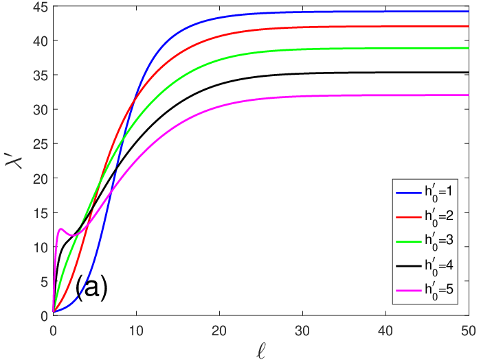
We present the $\ell$-dependence of coupling constants $\lambda^{\prime}$ and $h^{\prime}$ in Fig. 5. Both of $\lambda^{\prime}$ and $h^{\prime}$ flow to certain finite constants in the lowest energy limit, namely $\lambda^{\prime}\rightarrow\lambda^{\prime\ast}$ and $h^{\prime}\rightarrow h^{\prime\ast}$. Thus, $\lambda^{\prime}$ and $h^{\prime}$ are both marginal. The values of $\lambda^{\prime\ast}$ and $h^{\prime\ast}$ depend on the bare values of $\lambda^{\prime}$ and $h^{\prime}$. The flowing behavior of $C_{i}$ with $i=1,2,..,8$ in Figs. 2(a)-(h), respectively. According to Figs. 2(a), (b), and (c), we observe that $C_{1}$, $C_{2}$, and $C_{3}$ flow to zero very quickly. As a result, the parameters $c_{f}$ and $A$ do not receive singular renormalization, but flow to finite constants. The anomalous dimension of fermion field is given by $\eta_{f}=C_{1}$. Since $C_{1}$ vanishes rapidly at low energies, we infer that the fermion field does not acquire any anomalous dimension. The flow equation of quasiparticles residue $Z_{f}$ is

As shown in Fig. (6), $Z_{f}$ always flows to a finite constant in the lowest energy limit. These results indicate that the anisotropic Weyl fermions are well-defined quasiparticles and have a long lifetime at the SM-SC QCP.

We now analyze the impact of Yukawa coupling on the bosonic mode. Figs. 2(d)-(f) show that

in the lowest energy limit. The RG equation for parameter $c_{bz}$ becomes

The one-loop order correction does not lead to qualitative change of the flow of $c_{b\bot}$. Therefore, the bosonic SC fluctuation is anisotropically screened. Since $C_{4}$ flows to a finite value at low energies, the boson field $\phi$ acquires a finite anomalous dimension. Now the renormalized boson propagator becomes

where $q_{\perp}^{2}=q_{x}^{2}+q_{y}^{2}$.

According to Figs. 2(g) and (h), we see that $C_{7}\rightarrow 0$ and $C_{8}\rightarrow 0.5$ in the lowest energy limit. Combining Eq. (21), Eq. (22), and the low-energy behavior of $C_{1}$, $C_{4}$, $C_{7}$, and $C_{8}$, we conclude that the beta functions of $\lambda^{\prime}$ and $h^{\prime}$ vanish, which explains why both $\lambda^{\prime}$ and $h^{\prime}$ approach finite constants.

To understand the peculiarity of our result, we now compare it to previous studies of various quantum critical systems. Superconductivity was proposed to occur in several SM materials, including 2D Dirac SM [55, 56, 57, 58, 59], Luttinger SM [50], and 3D Weyl SM [60]. In 2D Dirac SM and Luttinger SM, the system flows to a stable infrared fixed point at the SC QCP. At such a fixed point, the fermion field acquires a finite anomalous dimension, which leads to power-law correction to the fermion DOS. Moreover, the fermion damping rate behaves as $\Gamma(\omega)\propto|\omega|^{1-\eta_{f}}$ at low energies, and the residue $Z_{f}\sim|\omega|^{\eta_{f}}\rightarrow 0$ in the limit $\omega\rightarrow 0$. In the case of 3D Weyl SM, the anomalous dimension of fermion field approaches to zero very slowly at the SC QCP [60]. Then, the fermion DOS receives logarithmic-like correction. Accordingly, the residue $Z_{f}$ also flows to zero very slowly, and the fermion damping rate exhibits marginal Fermi liquid behavior. We thus see that FL theory breaks down at the SM-SC QCP in all these systems. The singular fermion DOS revealed in previous theoretical works can be verified by scanning tunneling microscope (STM) measurements. In addition, angle resolved photoemission spectroscopy (ARPES) experiments [65] may be applied to probe the strong NFL behavior.

Similar NFL-like quantum critical phenomena also emerge in metals that are tuned to the vicinity of a continuous quantum phase transition. It is well-established that NFL behavior is realized near the FM, AFM, and nematic QCPs. For instance, the zero-$T$ Landau damping rate is $\Gamma(\omega)\propto|\omega|^{1/2}$ at an AFM QCP [19, 20] and $\Gamma(\omega)\propto|\omega|^{2/3}$ at an FM or Ising-type nematic QCPs [16, 22]. The corresponding residue $Z_{f}=0$ at all of these QCPs.

Different from the above quantum critical systems, the fermion anomalous dimension flows to zero very quickly and the residue $Z_{f}\neq 0$ at the SC QCP in 3D AWSM. It thus turns out that such QCP exhibits a trivial quantum criticality. Nevertheless, it is the triviality that makes this system distinctive. As shown in Fig. 1(a), a finite NFL regime exists on the phase diagram of conventional quantum critical systems. There is no such NFL regime in the system considered in this work. We observe from Fig. 1(b) that, although there is a clear QCP between the gapless SM phase and gapped SC phase, the anisotropic Weyl fermions do not display NFL behavior around this QCP. The vanishing of fermion anomalous dimension is closely related to the unusual anisotropic screening of the SC quantum fluctuation, which in turn is induced by the special dispersion of anisotropic Weyl fermions. Therefore, it is the strong anisotropy of fermion dispersion that distinguishes the 3D AWSM from all the other quantum critical systems. Indeed, if the fermion dispersion took a different form, the SC quantum fluctuation might lead to NFL-like quantum critical phenomena.

The trivial quantum criticality can be probed by measuring some observable quantities. In the non-interacting limit, the fermion DOS depends on energy as

and the specific heat depends on $T$ as

Since $c_{f}$ and $A$ are not singularly renormalized, both $\rho(\omega)$ and $C_{V}(T)$ exhibit qualitatively the same behavior as the free fermion gas at the SM-SC QCP. Additionally, because the residue $Z_{f}$ always takes a finite value, the fermion spectral function should have a sharp peak. This feature can be readily detected by ARPES experiments [65].

In summary, we have studied the influence of quantum critical fluctuation of SC order parameter on the low-energy behavior of fermions in 3D AWSM. Different from other quantum critical systems, the anomalous dimension of anisotropic Weyl fermions flows to zero quickly at low energies at the SM-SC QCP. As a consequence, the fermion residue is always finite, indicating the validity of FL description and the irrelevance of SC order parameter fluctuation. It turns out that the crucial physics of the SM-SC quantum phase transition can be captured by the simple mean-field analysis.

In a recent work, Yang et al. [63] demonstrated that the long-range Coulomb interaction is an irrelevant perturbation in 3D AWSM. Combining their results with ours, we conclude that 3D AWSM is an unusual system in which the fermions are extremely robust against repulsive long-range interactions. The stability of the system is guaranteed by the special dispersion of anisotropic Weyl fermions.

The 3D AWSM state could be realized either at the QCP between band-insulator and ordinary 3D WSM, or at the QCP between band-insulator and 3D topological insulator in some non-centrosymmetric systems [64]. For instance, it is predicted that the 3D AWSM state may be achieved by applying pressure to the compound BiTeI, in which the inversion symmetry is broken [62, 66]. Experiments performed in pressured BiTeI by means of X-ray powder diffraction and infrared spectroscopy are consistent with these theoretical predictions [67]. Recent Shubnikov-de Haas quantum oscillation experiments have revealed evidence of a pressure-induced topological quantum phase transition in BiTeI [68]. Once superconductivity is induced by certain mechanism in the mother 3D AWSM state, it should be possible to measure some observable quantities, such as the fermion spectral function and specific heat, to verify whether the anisotropic Weyl fermions behave as free fermion gas at the SM-SC QCP and also in the SM phase.

We would like to acknowledge the financial support by the National Natural Science Foundation of China under Grants 11574285 and 11504379. J.R.W. is partly supported by the Natural Science Foundation of Anhui Province under Grant 1608085MA19. X.L. and G.-Z.L. are partly supported by the Fundamental Research Funds for the Central Universities (P. R. China) under Grant WK2030040085.

References

• [1] G. F. Giuliani and G. Vignale, Quantum Theory of the Electron Liquid (Cambridge University Press, Cambridge, 2005).
• [2] P. Coleman, Introduction to Many-Body Physics (Cambridge University Press, Cambridge, 2015).
• [3] R. Shankar, Rev. Mod. Phys. 66, 129 (1994).
• [4] T. Holstein, R. E. Norton, and P. Pincus, Phys. Rev. B 8, 2649 (1973).
• [5] P. A. Lee, Phys. Rev. Lett. 63, 680 (1989).
• [6] P. A. Lee and N. Nagaosa, Phys. Rev. B 46, 5621 (1992).
• [7] J. Gan and E. Wong, Phys. Rev. Lett. 71, 4226 (1993).
• [8] B. L. Altshuler, L. B. Ioffe, and A. J. Millis, Phys. Rev. B 50, 14048 (1994).
• [9] J. Polchinski, Nucl. Phys. B 422, 617 (1994).
• [10] S.-S. Lee, Phys. Rev. B 80, 165102 (2009).
• [11] C. M. Varma, Z. Nussinov, and W. v. Saarloos, Phys. Rep. 361, 267 (2002).
• [12] H. v. Löhneysen, A. Rosch, M. Vojta, and P. Wölfle, Rev. Mod. Phys. 79, 1015 (2007).
• [13] J. A. Hertz, Phys. Rev. B 14, 1165 (1976).
• [14] A. J. Millis, Phys. Rev. B 48, 7183 (1993).
• [15] S. Sachdev, Rev. Mod. Phys. 75, 913 (2003).
• [16] J. Rech, C. Pépin, and A. V. Chubukov, Phys. Rev. B 74, 195126 (2006).
• [17] S. P. Ridgway and C. A. Hooley, Phys. Rev. Lett 114, 226404 (2015).
• [18] X. Y. Xu, K. Sun, Y. Schattner, E. Berg, and Z. Y. Meng, Phys. Rev. X 7, 031058 (2017).
• [19] A. Abanov, A. V. Chubukov, and J. Schmalian, Adv. Phys. 52, 119 (2003).
• [20] M. A. Metlitski and S. Sachdev, Phys. Rev. B 82, 075128 (2010).
• [21] A. Schlief, P. Lunts, and S.-S. Lee, Phys. Rev. X 7, 021010 (2017).
• [22] W. Metzner, D. Rohe, and S. Andergassen, Phys. Rev. Lett. 91, 066402 (2003).
• [23] M. A. Metlitski and S. Sachdev, Phys. Rev. B 82, 075127 (2010).
• [24] M. Garst and A. V. Chubukov, Phys. Rev. B 81, 235105 (2010).
• [25] S. Lederer, Y. Schattner, E. Berg, and S. A. Kivelson, Proc. Natl. Acad. Sci. U.S.A. 114, 4905 (2017).
• [26] O. Vafek and A. Vishwanath, Annu. Rev. Condens. Matter Phys. 5, 83 (2014).
• [27] T. O. Wehling, A. M. Black-Schaffer, and A. V. Balatsky, Adv. Phys. 63, 1 (2014).
• [28] N. P. Armitage, E. J. Mele, and A. Vishwanath, Rev. Mod. Phys. 90, 015001 (2018).
• [29] A. A. Burkov, Nat. Mater. 15, 1145 (2016).
• [30] B. Yan and C. Felser, Annu. Rev. Condens. Matter Phys. 8, 337 (2017).
• [31] M. Z. Hasan, S.-Y. Xu, I. Belopolski, and S.-M. Huang, Annu. Rev. Condens. Matter Phys. 8, 289 (2017).
• [32] H. Weng, X. Dai, and Z. Fang, J. Phys.: Condens. Matter 28, 303001 (2016).
• [33] C. Fang, H. Weng, X. Dai, and Z. Fang, Chin. Phys. B 25, 117106 (2016).
• [34] V. N. Kotov, B. Uchoa, V. M. Pereira, F. Guinea, and A. H. Castro Neto, Rev. Mod. Phys. 84, 1067 (2012).
• [35] B. Uchoa, G. G. Cabrera, and A. H. Castro Neto, Phys. Rev. B 71, 184509 (2005).
• [36] E. Zhao and A. Paramekanti, Phys. Rev. Lett. 97, 230404 (2006).
• [37] B. Uchoa and A. H. Castro Neto, Phys. Rev. Lett. 98, 146801 (2007).
• [38] N. B. Kopnin and E. B. Sonin, Phys. Rev. Lett. 100, 246808 (2008).
• [39] C. Honerkamp, Phys. Rev. Lett. 100, 146404 (2008).
• [40] B. Roy and I. F. Herbut, Phys. Rev. B 82, 035429 (2010).
• [41] B. Roy, V. Juričić, and I. F. Herbut, Phys. Rev. B 87, 041401(R) (2013).
• [42] R. Nandkishore, J. Maciejko, D. A. Huse, and S. L. Sondhi, Phys. Rev. B 87, 174511 (2013).
• [43] J. Wang, P.-L. Zhao, J.-R. Wang, and G.-Z. Liu, Phys. Rev. B 95, 054507 (2017).
• [44] B. Roy and S. Das Sarma, Phys. Rev. B 94, 115137 (2016).
• [45] T. Meng and L. Balents, Phys. Rev. B 86, 054504 (2012).
• [46] J. Maciejko and R. Nandkishore, Phys. Rev. B 90, 035126 (2014).
• [47] H. Wei, S.-P. Chao, and V. Aji, Phys. Rev. B 89, 014506 (2014).
• [48] S. Sur and R. Nandkishore, New J. Phys. 18, 115006 (2016).
• [49] B. Roy, Phys. Rev. B 96, 041113(R) (2017).
• [50] I. Boettcher and I. F. Herbut, Phys. Rev. B 93, 205138 (2016).
• [51] I. Boettcher and I. F. Herbut, Phys. Rev. Lett. 120, 057002 (2018).
• [52] I. Mandal, Ann. Phys. (New York) 392, 179 (2018).
• [53] B. Uchoa and K. Seo, Phys. Rev. B 96, 220503(R) (2017).
• [54] B. Roy and M. S. Foster, Phys. Rev. X 8, 011049 (2018).
• [55] S.-S. Lee, Phys. Rev. B 76, 075103 (2007).
• [56] P. Ponte and S.-S. Lee, New J. Phys. 16, 013044 (2014).
• [57] T. Grover, D. N. Sheng, and A. Vishwanath, Science 344, 280 (2014).
• [58] W. Witczak-Krempa and J. Maciejko, Phy. Rev. Lett. 116, 100402 (2016).
• [59] N. Zerf, C.-H. Lin, and J. Maciejko, Phys. Rev. B 94, 205106 (2016).
• [60] S.-K. Jian, Y.-F. Jiang, and H. Yao, Phys. Rev. Lett. 114, 237001 (2015).
• [61] S.-K. Jian, C.-H. Lin, J. Maciejko, and H. Yao, Phys. Rev. Lett. 118, 166802 (2017).
• [62] B.-J. Yang, M. S. Bahramy, R. Arita, H. Isobe, E.-G. Moon, and N. Nagaosa, Phys. Rev. Lett. 110, 086402 (2013).
• [63] B.-J. Yang, E.-G. Moon, H. Isobe, and N. Nagaosa, Nat. Phys. 10, 774 (2014).
• [64] B.-J. Yang and N. Nagaosa, Nat. Commun. 5, 4898 (2014).
• [65] A. Damascelli, Z. Hussain, and Z.-X. Shen, Rev. Mod. Phys. 75, 473 (2003).
• [66] M. S. Bahramy, B.-J. Yang, R. Arita, and N. Nagaosa, Nat. Commun. 3, 679 (2012).
• [67] X. Xi, C. Ma, Z. Liu, Z. Chen, W. Ku, H. Berger, C. Martin, D. B. Tanner, and G. L. Carr, Phys. Rev. Lett. 111, 155701 (2013).
• [68] J. Park, K.-H. Jin, Y. J. Jo, E. S. Choi, W. Kang, E. Kampert, J.-S. Rhyee, S.-H. Jhi, and J. S. Kim, Sci. Rep. 5, 15973 (2015).