跳到论文正文
W Papers独立论文阅读器 arXiv:1801.05593 论文正文 计算阅读时间 · 0%
引用这篇论文根据当前论文元数据生成,正式投稿前建议核对。


License: arXiv.org perpetual non-exclusive license
arXiv:1801.05593v2 [math.CO] 27 Sep 2018

Relation between combinatorial Ricci curvature and Lin-Lu-Yau’s Ricci Curvature on cell complexes

Kazuyoshi Watanabe    Taiki Yamada
Abstract.

In this paper we compare the combinatorial Ricci curvature on cell complexes and Lin-Lu-Yau’s Ricci curvature defined on graphs. On a cell complex, the combinatorial Ricci curvature is introduced by the Bochner-Weitzenböck formula. A cell complex corresponds to a graph such that the vertices are cells and the edges are vectors on the cell complex. We compare these two kinds of Ricci curvatures by the coupling and the Kantorovich duality.

††footnotetext: Mathematics Subject Classification: Primary 05E45; Secondary 53B21.††footnotetext: Key words and phrases: Graph theory, Optimal transport, Cell complex, Ricci curvature.

Tohoku University

1 Introduction

In the Riemannian geometry, the curvature plays an important role. Especially the Ricci curvature is studied in geometric analysis on Riemannian manifolds and there are many results on manifolds with non-negative Ricci curvature or with the Ricci curvature bounded below. In the analysis of the Ricci curvature the Bochner-Weitzenböck formula is useful. This formula gives a relation between the curvature tensor and the Hodge Laplacian on smooth differential forms.

There are some definitions of generalized Ricci curvature, one of which is Ollivier’s coarse Ricci curvature (see [7]). It is formulated by the 1-Wasserstein distance on a metric space (X,d)(X,d) with a random walk m={mx}x∈Xm=\left\{m_{x}\right\}_{x\in X}, where mxm_{x} is a probability measure on XX. The coarse Ricci curvature is defined as, for two distinct points x,y∈Xx,y\in X,

κ⁡(x,y):=1−W⁡(mx,my)d⁡(x,y),\displaystyle\kappa(x,y):=1-\cfrac{W(m_{x},m_{y})}{d(x,y)},

where WW(mx,mym_{x},m_{y}) is the 11-Wasserstein distance between mxm_{x} and mym_{y}. In 2010, Lin, Lu and Yau [5] modified the definition of Ollivier’s coarse Ricci curvature on graphs. They showed some properties about this curvature, such as the Cartesian product and Erdös-Renyi’s random graph. In 2012, Jost and Liu [4] studied the relation between the Ricci curvature and the local clustering coefficient. Recently, the Ricci curvature on graphs was applied to directed graph [10], internet topology and so on. In this paper, we call this Ricci curvature the LLY-Ricci curvature, and denote it by κ\kappa.

On the other hand, a cell complex is studied as a combinatorial space and applied to various works. In a recent work, Forman established some discrete analogues of differential geometry to cell complexes. In [3], the discrete Morse theory was established and the Morse inequality, which is the relation between critical cells and the homology of the cell complex, was constructed. The theory has various practical applications in diverse fields of applied mathematics and computer science. By using the discrete vector field the discrete Morse theory is extended to the discrete Novikov-Morse theory [2], and in this theory he defined a differential form on the cell complex. A differential form is not defined as the cochain of the cell complex but as a linear map on the chain of the cell complex.

In [9], the first name author introduce the definition of the combinatorial Ricci curvature on a cell complex by the Bochner-Weitzenböck formula on combinatorial differential forms. A combinatorial 1-form ω\omega has a value at a pair of cells (τ>σ)(\tau>\sigma) and we call such a pair (τ>σ)(\tau>\sigma) a vector provided that σ\sigma is a face of τ\tau and dim⁡σ+1=dim⁡τ\operatorname{dim}\sigma+1=\operatorname{dim}\tau. For the definition of the covariant derivative |∇ω||\nabla\omega| of a combinatorial 1-form, we present the parallel vectors, that are called by 0- and 2-neighbor vectors. We define the covariant of a 1-form |∇ω||\nabla\omega| and the Laplacian for the absolute value of combinatorial 1-form Δ♭​|ω|2\varDelta^{\flat}|\omega|^{2} as the difference between the components of parallel vectors. Then we define the combinatorial Ricci curvature by

Ric⁡(ω)​(τ>σ)=⟨Δ​ω,ω⟩​(τ>σ)−12​|∇ω|2​(τ>σ)+12​Δ♭​|ω|2​(τ>σ).\displaystyle\operatorname{Ric}(\omega)(\tau>\sigma)=\langle\varDelta\omega,\omega\rangle(\tau>\sigma)-\frac{1}{2}|\nabla\omega|^{2}(\tau>\sigma)+\frac{1}{2}\varDelta^{\flat}|\omega|^{2}(\tau>\sigma). (1)

For a graph and for a 2-dimensional cell complex decomposing a closed surface, we have the Gauss-Bonnet theorem for this combinatorial Ricci curvature [9].

For a cell complex MM, we consider the graph GMG_{M} such that the set of vertices of GMG_{M} is the set of cells in MM, and the set of edges of GMG_{M} is the set of vectors in MM. We call GMG_{M} the corresponding graph to a cell complex MM.

We study the relationship between our combinatorial Ricci curvature on MM and the LLY-Ricci curvature on GMG_{M}. The LLY-Ricci curvature is defined by the Wasserstein distance between probability measures. One of our main theorems is stated as follows.

Let τp+1\tau^{p+1} and σp\sigma^{p} respectively be a (p+1)(p+1)-cell and a pp-cell of MM such that τ>σ\tau>\sigma. Then we have

κ⁡(τ,σ)=Ric⁡(τ>σ)dτ∨dσ+2​(1dτ∧dσ−1dτ∨dσ)+dτ∧dσdτ∨dσ−1,\displaystyle\kappa(\tau,\sigma)=\frac{\operatorname{Ric}(\tau>\sigma)}{d_{\tau}\vee d_{\sigma}}+2\left(\frac{1}{d_{\tau}\wedge d_{\sigma}}-\frac{1}{d_{\tau}\vee d_{\sigma}}\right)+\frac{d_{\tau}\wedge d_{\sigma}}{d_{\tau}\vee d_{\sigma}}-1, (2)

where dτ∧dσ=min⁡{dτ,dσ}d_{\tau}\wedge d_{\sigma}=\min\{d_{\tau},d_{\sigma}\} and dσ∨dσ=max⁡{dτ,dσ}d_{\sigma}\vee d_{\sigma}=\max\{d_{\tau},d_{\sigma}\}.

For the estimate of a lower bound of the LLY-Ricci curvature, we construct the coupling between two probability measures around cells. Since the supports of two probability measures do not intersect each other, this coupling is calculated by combinatorially. Moreover we estimate an upper bound of the LLY-Ricci curvature by using the combinatorial Ricci curvature. From the Kantorovich duality, a 1-Lipschitz function gives the lower bound of the Wasserstein distance between probability measures. Since two bounds coincide with each other, we prove Theorem 1.

In section 5, we see that the LLY-Ricci curvature gives the lower bound of the first nonzero eigenvalue of the Laplacian on a cell complex. By applying the Kantorovich duality to the eigenfunction with respect to the first nonzero eigenvalue we estimate the Wasserstein distance between two probability measures. The estimate is useful for computing practical cell complexes. Actually we see the example of a cell complex with the positive combinatorial Ricci curvature, and check the lower estimation of the first nonzero eigenvalue of the Laplacian.

Acknowledgment

The authors thank their supervisors, Professor Takashi Shioya, for his continuous support and providing important comments. They also thank the referee for his/her valuable comments and suggestions.

2 Definition of combinatorial Ricci curvature

2.1 Combinatorial differential form

In this section, we present a differential form on a cell-complex introduced in [2]. Let MM be a cell complex. For cells σ\sigma and τ\tau, we write σ<τ\sigma<\tau or τ>σ\tau>\sigma if σ\sigma is contained in the boundary of τ\tau. First, we define a regular cell complex.

We say MM is a regular cell complex, if for each p-cell σ\sigma of MM the characteristic map hσ:ep→Mh_{\sigma}:e^{p}\to M maps epe^{p} homeomorphically onto its image, where epe^{p} is a closed ball in the p-dim Euclidean space. Throughout the paper, we always assume that MM is a regular cell complex. If not, it will be clearly stated. Let the dimension of MM be nn, and

0⟶Cn(M)⟶∂Cn−1(M)⟶∂⋯⟶∂C0(M)⟶0\displaystyle 0\longrightarrow C_{n}(M)\overset{\partial}{\longrightarrow}C_{n-1}(M)\overset{\partial}{\longrightarrow}\cdots\overset{\partial}{\longrightarrow}C_{0}(M)\longrightarrow 0 (3)

be the real cellular chain complex of MM. We set

C∗​(M)=⨁pCp​(M).\displaystyle C_{*}(M)=\bigoplus_{p}C_{p}(M). (4)

A linear map ω:C∗​(M)→C∗​(M)\omega:C_{*}(M)\rightarrow C_{*}(M) is said to be of degree dd if for all p=1,…,np=1,...,n,

ω⁡(Cp​(M))⊂Cp−d​(M).\displaystyle\omega(C_{p}(M))\subset C_{p-d}(M). (5)

We say that a linear map ω\omega of degree dd is l​o​c​a​llocal if, for each pp and each oriented pp-cell α\alpha, ω⁡(α)\omega(\alpha) is a linear combination of oriented (p−dp-d)-cells that are faces of α\alpha.

For d≥0d\geq 0, we say that a local linear map ω:C∗​(M)→C∗​(M)\omega:C_{*}(M)\rightarrow C_{*}(M) of degree dd is a combinatorial differential dd-form, and we denote the space of combinatorial differential dd-forms by Ωd​(M)\varOmega^{d}(M). We define the differential of combinatorial differential forms

d:Ωd​(M)→Ωd+1​(M)\displaystyle d:\varOmega^{d}(M)\rightarrow\varOmega^{d+1}(M) (6)

as follows. For any ω∈Ωd​(M)\omega\in\varOmega^{d}(M) and any pp-chain cc, we define (d​ω)​(c)∈Cp−(d+1)​(M)(d\omega)(c)\in C_{p-(d+1)}(M) by

(d​ω)​(c)=∂(ω⁡(c))−(−1)d​ω​(∂c).\displaystyle(d\omega)(c)=\partial(\omega(c))-(-1)^{d}\omega(\partial c). (7)

That is,

dω=∂∘ω−(−1)dω∘∂.\displaystyle d\omega=\partial\circ\omega-(-1)^{d}\omega\circ\partial. (8)

Let us define an inner product on C∗​(M)C_{*}(M). For any two pp-cells σ,σ′\sigma,\sigma^{\prime}, we set an inner product as

⟨σ,σ′⟩=δσ,σ′,\displaystyle\langle\sigma,\sigma^{\prime}\rangle=\delta_{\sigma,\sigma^{\prime}}, (9)

where δσ,σ′\delta_{\sigma,\sigma^{\prime}} is the Kronecker delta, that is, δσ,σ′=1\delta_{\sigma,\sigma^{\prime}}=1 for σ=σ′\sigma=\sigma^{\prime} and the others are 0. We define the L2L^{2} inner product for combinatorial differential forms. For two dd-forms u,vu,v, we set

⟨u,v⟩=∑σ⟨u⁡(σ),v⁡(σ)⟩,\displaystyle\langle u,v\rangle=\sum_{\sigma}\langle u(\sigma),v(\sigma)\rangle, (10)

where the sum is taken over all cells σ\sigma in MM.
Let us consider the adjoint operator of differential with respect to the inner product,

d∗:Ωd​(M)→Ωd−1​(M).\displaystyle d^{*}:\varOmega^{d}(M)\rightarrow\varOmega^{d-1}(M). (11)

That is, for a dd-form uu and a (d−1)(d-1)-form vv we have

⟨d∗​u,v⟩=⟨u,d​v⟩.\displaystyle\langle d^{*}u,v\rangle=\langle u,dv\rangle. (12)

We define the Laplacian for combinatorial differential forms by

Δ=d​d∗+d∗​d.\displaystyle\varDelta=dd^{*}+d^{*}d. (13)

2.2 Combinatorial function and 1-form on cell complexes

We realize a combinatorial 0-form as a function. We take a 0-form f∈Ω0​(M)f\in\varOmega^{0}(M), that is,

f:C∗​(M)→C∗​(M).\displaystyle f:C^{*}(M)\rightarrow C^{*}(M). (14)

For any cell σ\sigma, we have

f⁡(σ)=fσ​σ,\displaystyle f(\sigma)=f_{\sigma}\sigma, (15)

and consider fσ∈𝐑f_{\sigma}\in\mathbf{R} as the value of the function ff. For a pp-dimensional cell τ\tau, the derivative of ff is

df(τ)=∑σ:τ>σ(fτ−fσ)(−1)τ>σσ,\displaystyle df(\tau)=\sum_{\sigma:\tau>\sigma}(f_{\tau}-f_{\sigma})(-1)^{\tau>\sigma}\sigma, (16)

where the sum is taken over all (p−1)(p-1)-dimensional cells σ\sigma that are faces of τ\tau, and (−1)τ>σ(-1)^{\tau>\sigma} is the incidence number between τ\tau and σ\sigma.

Let ω∈Ω1​(M)\omega\in\varOmega^{1}(M) be a combinatorial 1-form. For a pp-dimensional cell τ\tau, we set

ω(τ)=∑σ:τ>σωστ(−1)τ>σσ,\displaystyle\omega(\tau)=\sum_{\sigma:\tau>\sigma}\omega^{\tau}_{\sigma}(-1)^{\tau>\sigma}\sigma, (17)

where the sum is taken over all (p−1)(p-1)-dimensional cells σ\sigma that are faces of τ\tau, and (−1)τ>σ(-1)^{\tau>\sigma} is the incidence number between τ\tau and σ\sigma. We call the pair (τ>σ)(\tau>\sigma) a vector provided that a pp-dimensional cell σ\sigma is a face of (p+1)(p+1)-dimensional cell τ\tau. We say that ω\omega has the value ωστ\omega^{\tau}_{\sigma} at the vector (τ>σ)(\tau>\sigma).

For any cell σ\sigma, the dual derivative of ω\omega is

d∗​(ω)​(σ)\displaystyle d^{*}(\omega)(\sigma) =\displaystyle= ∂∗(ω⁡(σ))−ω⁡(∂∗(σ))\displaystyle\partial^{*}(\omega(\sigma))-\omega(\partial^{*}(\sigma)) (18)
=\displaystyle= −∑τp+1:τ>σωτσ+∑ρp−1:ρ<σωσρ,\displaystyle-\sum_{\tau^{p+1}:\tau>\sigma}\omega^{\tau}_{\sigma}+\sum_{\rho^{p-1}:\rho<\sigma}\omega^{\sigma}_{\rho}, (19)

where the first sum is taken over all (p+1)(p+1)-dimensional cells τ\tau that have σ\sigma as a face, and the second sum is over all (p−1)(p-1)-dimensional cells ρ\rho that are the faces of σ\sigma.

Then for any cell σ\sigma, the Laplacian of combinatorial function ff is represented by

Δ​f​(σ)\displaystyle\varDelta f(\sigma) =\displaystyle= d∗​d​f​(σ)\displaystyle d^{*}df(\sigma) (20)
=\displaystyle= −∑τp+1:τ>σdfτσ+∑ρp−1:ρ<σdfσρ\displaystyle-\sum_{\tau^{p+1}:\tau>\sigma}df^{\tau}_{\sigma}+\sum_{\rho^{p-1}:\rho<\sigma}df^{\sigma}_{\rho} (21)
=\displaystyle= −∑τp+1;τ>σ(fτ−fσ)+∑ρp−1;σ>ρ(fσ−fρ).\displaystyle-\sum_{\tau^{p+1};\tau>\sigma}(f_{\tau}-f_{\sigma})+\sum_{\rho^{p-1};\sigma>\rho}(f_{\sigma}-f_{\rho}). (22)

2.3 Combinatorial Ricci curvature

Let MM be a regular cell complex. We say that MM is quasiconvex if for every two distinct (p+1)(p+1)-cells τ1\tau_{1} and τ2\tau_{2} of MM, if τ1¯∩τ2¯\bar{\tau_{1}}\cap\bar{\tau_{2}} contains a pp-cell σ\sigma, then τ1¯∩τ2¯=σ¯\bar{\tau_{1}}\cap\bar{\tau_{2}}=\bar{\sigma}. In particular this implies that τ1¯∩τ2¯\bar{\tau_{1}}\cap\bar{\tau_{2}} contains at most one pp-cell.

Refer to caption

]Non quasiconvex

Refer to caption

]Quasiconvex

Let MM be a regular quasiconvex cell complex. We consider “parallel vectors”, which yield the covariant derivative of a combinatorial 1-form.

Let τ,σ\tau,\sigma be two cells of MM such that the dimension is (p+1)(p+1) and pp respectively and σ\sigma is a face of τ\tau.

We define 0-neighbor vectors of (τ>σ)(\tau>\sigma) as the following.

  • •

    vectors (τ′>σ)(\tau^{\prime}>\sigma) for (p+1)(p+1)-cells τ′≠τ\tau^{\prime}\neq\tau such that there are no (p+2)(p+2)-cell μ\mu such that μ>τ,τ′\mu>\tau,\tau^{\prime}.

  • •

    vectors (τ>σ′)(\tau>\sigma^{\prime}) for pp-cells σ′≠σ\sigma^{\prime}\neq\sigma such that there are no (p−1)(p-1)-cell ρ\rho such that σ,σ′>ρ\sigma,\sigma^{\prime}>\rho.

We define 2-neighbor vectors of (τ>σ)(\tau>\sigma) as the following.

  • •

    vectors (μ>τ′)(\mu>\tau^{\prime}) for (p+1),(p+2)(p+1),(p+2)-cells τ′\tau^{\prime} and μ\mu such that μ>τ>σ\mu>\tau>\sigma, μ>τ′>σ\mu>\tau^{\prime}>\sigma and τ≠τ′\tau\neq\tau^{\prime}.

  • •

    vectors (σ′>ρ)(\sigma^{\prime}>\rho) for (p−1),p(p-1),p-cells ρ\rho and σ′\sigma^{\prime} such that τ>σ>ρ\tau>\sigma>\rho, τ>σ′>ρ\tau>\sigma^{\prime}>\rho and σ≠σ′\sigma\neq\sigma^{\prime}.

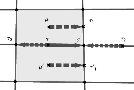
These ideas and names are based on [1]. In Figure 3, there exists a 2-form (μ→σ\mu\to\sigma) between (τ>σ)(\tau>\sigma) and (μ>τ1\mu>\tau_{1}), so we call the vector (μ>τ1\mu>\tau_{1}) a 2-neighbor vector. In the same way, the vector (μ′>τ1′\mu^{\prime}>\tau^{\prime}_{1}) is also a 2-neighbor vector. On the other hand, there exists a 0-form (σ→σ)(\sigma\to\sigma) between (τ>σ)(\tau>\sigma) and (τ2>σ\tau_{2}>\sigma), so we call the vector (τ2>σ\tau_{2}>\sigma) a 0-neighbor vector. The vector (τ>σ2\tau>\sigma_{2}) is also a 0-neighbor vector.

Refer to caption

]0- and 2- neighbor vectors

For a combinatorial 1-form ω\omega on MM, we define the combinatorial covariant derivative as

|∇ω|2​(τ>σ)\displaystyle|\nabla\omega|^{2}(\tau>\sigma) =\displaystyle= ∑(μ>τ′);2−neighbor(ωστ−ωτ′μ)2+∑(σ′>ρ);2−neighbor(ωστ−ωρσ′)2\displaystyle\sum_{(\mu>\tau^{\prime});{\rm 2-neighbor}}(\omega^{\tau}_{\sigma}-\omega^{\mu}_{\tau^{\prime}})^{2}+\sum_{(\sigma^{\prime}>\rho);{\rm 2-neighbor}}(\omega^{\tau}_{\sigma}-\omega^{\sigma^{\prime}}_{\rho})^{2} (23)
+\displaystyle+ ∑(τ′>σ);0−neighbor(ωστ+ωστ′)2+∑(τ>σ′);0−neighbor(ωστ+ωσ′τ)2,\displaystyle\sum_{(\tau^{\prime}>\sigma);{\rm 0-neighbor}}(\omega^{\tau}_{\sigma}+\omega^{\tau^{\prime}}_{\sigma})^{2}+\sum_{(\tau>\sigma^{\prime});{\rm 0-neighbor}}(\omega^{\tau}_{\sigma}+\omega^{\tau}_{\sigma^{\prime}})^{2}, (24)

where the sums are taken over all 2-neighbor vectors and 0-neighbor vectors for (τ>σ)(\tau>\sigma) respectively.

For a combinatorial 1-form ω\omega on MM, we define the Laplacian of |ω|2|\omega|^{2} as

Δ♭​|ω|2​(τ>σ)=∑(μ>τ′);2−neighbor((ωστ)2−(ωτ′μ)2)+∑(σ′>ρ);2−neighbor((ωστ)2−(ωρσ′)2)\displaystyle\varDelta^{\flat}|\omega|^{2}(\tau>\sigma)=\sum_{(\mu>\tau^{\prime});{\rm 2-neighbor}}((\omega^{\tau}_{\sigma})^{2}-(\omega^{\mu}_{\tau^{\prime}})^{2})+\sum_{(\sigma^{\prime}>\rho);{\rm 2-neighbor}}((\omega^{\tau}_{\sigma})^{2}-(\omega^{\sigma^{\prime}}_{\rho})^{2}) (25)
+∑(τ′>σ);0−neighbor((ωστ)2−(ωστ′)2)+∑(τ>σ′);0−neighbor((ωστ)2−(ωσ′τ)2),\displaystyle+\sum_{(\tau^{\prime}>\sigma);{\rm 0-neighbor}}((\omega^{\tau}_{\sigma})^{2}-(\omega^{\tau^{\prime}}_{\sigma})^{2})+\sum_{(\tau>\sigma^{\prime});{\rm 0-neighbor}}((\omega^{\tau}_{\sigma})^{2}-(\omega^{\tau}_{\sigma^{\prime}})^{2}), (26)

where the sums are taken over all 2-neighbor vectors and 0-neighbor vectors for (τ>σ)(\tau>\sigma) respectively.

This Laplacian is symmetry for vectors, hence we have

∑(τ>σ)Δ♭​|ω|2​(τ>σ)=0,\displaystyle\sum_{(\tau>\sigma)}\varDelta^{\flat}|\omega|^{2}(\tau>\sigma)=0, (27)

where the sum is taken over all vectors.

For a combinatorial 1-form ω\omega, we define the combinatorial Ricci curvature on a vector (τ>σ)(\tau>\sigma) as

Ric⁡(ω)​(τ>σ)=⟨Δ​ω,ω⟩​(τ>σ)−12​|∇ω|2​(τ>σ)+12​Δ♭​|ω|2​(τ>σ).\displaystyle\operatorname{Ric}(\omega)(\tau>\sigma)=\langle\varDelta\omega,\omega\rangle(\tau>\sigma)-\frac{1}{2}|\nabla\omega|^{2}(\tau>\sigma)+\frac{1}{2}\varDelta^{\flat}|\omega|^{2}(\tau>\sigma). (28)

Let MM be a regular quasiconvex cell-complex, and (τ>σ)(\tau>\sigma) a vector on MM. For a combinatorial 1-form ω\omega on MM, the combinatorial Ricci curvature Ric⁡(ω)\operatorname{Ric}(\omega) is represented by

Ric⁡(ω)​(τ>σ)=(2−#⁡{0−neighbor​vector​of​(τ>σ)})​(ωστ)2.\displaystyle\operatorname{Ric}(\omega)(\tau>\sigma)=(2-\#\{{\rm 0-neighbor\ vector\ of\ }(\tau>\sigma)\})(\omega^{\tau}_{\sigma})^{2}. (29)

We define the combinatorial Ricci curvature on a vector as the one for a unit vector.

Let MM be a regular quasiconvex cell-complex, and (τ>σ)(\tau>\sigma) a vector on MM. We define the combinatorial Ricci curvature on a vector (τ>σ)(\tau>\sigma) by

Ric⁡(τ>σ)=(2−#⁡{0−neighbor​vector​of​(τ>σ)}).\displaystyle\operatorname{Ric}(\tau>\sigma)=(2-\#\{{\rm 0-neighbor\ vector\ of\ }(\tau>\sigma)\}). (30)

Let K1K^{1} be a 1-dimensional cell complex such that the set of vertices is {vi}i=−∞∞\{v_{i}\}_{i=-\infty}^{\infty} and the set of edges is {ei}i=−∞∞\{e_{i}\}_{i=-\infty}^{\infty}, and they are related by

vi<ei>vi+1.\displaystyle v_{i}<e_{i}>v_{i+1}. (31)

K1K^{1} is homeomorphic to a line. 0-neighbor vectors of (ei>vi)(e_{i}>v_{i}) are two vectors (ei−1>vi)(e_{i-1}>v_{i}) and (ei>vi+1)(e_{i}>v_{i+1}). Then the combinatorial Ricci curvature at the vectors (ei>vi)(e_{i}>v_{i}) on K1K^{1} is

Ric⁡(ei>vi)=Ric⁡(ei>vi+1)=0.\displaystyle\operatorname{Ric}(e_{i}>v_{i})=\operatorname{Ric}(e_{i}>v_{i+1})=0. (32)

We set an nn-dimensional cell complex KnK^{n} by the nn times product of K1K^{1}. Then KnK^{n} is homeomorphic to the Euclidean space 𝐑n{\bf R}^{n}, and each pp-cell of KnK^{n} is a pp-cube. We represent vertices of KnK^{n} as integer lattice points (m1,…,mn)(m_{1},...,m_{n}). We consider pp-cell τ=([0,1],…,[0,1],0,…,0)\tau=([0,1],...,[0,1],0,...,0), where first pp components are intervals and last n−pn-p components are points. Let σ=([0,1],…,[0,1],0,…,0)\sigma=([0,1],...,[0,1],0,...,0) be a (p−1)(p-1)-cell in τ\tau, where first p−1p-1 components are intervals and last n−p+1n-p+1 components are points. Then 0-neighbor vectors of (τ>σ)(\tau>\sigma) are two vectors (τ>([0,1],…,[0,1],1,0,…,0))(\tau>([0,1],...,[0,1],1,0,...,0)) and (([0,1],…,[0,1],[−1,0],0,…,0)>σ)(([0,1],...,[0,1],[-1,0],0,...,0)>\sigma). Similarly, the number of 0-neighbor vector of any vector vv on KnK^{n} is 2. Thus, for any vector vv on KnK^{n} the combinatorial Ricci curvature is

Ric⁡(v)=0.\displaystyle\operatorname{Ric}(v)=0. (33)

Thus KnK^{n} is a combinatorially flat space.

Refer to caption

]1-complex K1K^{1}

Refer to caption

]2-complex K2K^{2}

3 LLY-Ricci curvature on cell complexes

In [5], the LLY-Ricci curvature is defined on a graph by using the Wasserstein distance. For a cell complex MM we consider the corresponding graph GMG_{M}, i.e., the set of vertices of GMG_{M} is the set of cells in MM, and the set of edges of GMG_{M} is the set of vectors in MM.

Refer to caption

]Cell complex MM

Refer to caption

]Corresponding graph GMG_{M}

Then we define the LLY-Ricci curvature on the graph GMG_{M}. We denote the set of cells in MM by SS. We consider the distance and a probability measure μ\mu on a cell complex MM as the one on the corresponding graph GMG_{M}.

  1. (1)

    A directed path between σ∈S\sigma\in S and τ∈S\tau\in S is a sequence of edges
    {(ai,aOPENi+1)}i=0n−1\left\{(a_{i},a_{i+1)}\right\}_{i=0}^{n-1}, where a0=σa_{0}=\sigma, an=τa_{n}=\tau. We call nn the length of the path.

  2. (2)

    The distance d⁡(σ,τ)d(\sigma,\tau) between two cells σ,τ∈S\sigma,\tau\in S is given by the length of a shortest directed path from σ\sigma to τ\tau.

  3. (3)

    For any σ∈S\sigma\in S, the neighborhood of σ\sigma is defined as

    Γ⁡(σ)={c∈M∣c=τp+1​with​τ>σ​or​c=ρp−1​with​ρ<σ}.\displaystyle\varGamma(\sigma)=\left\{c\in M\mid c=\tau^{p+1}~{\rm with}~\tau>\sigma~{\rm or}~c=\rho^{p-1}~{\rm with}~\rho<\sigma\right\}.

For any α∈[0,1]\alpha\in[0,1], and for any pp-cell σ\sigma in MM, we define a probability measure mσαm^{\alpha}_{\sigma} on MM by

mσα​(c)={α,if​c=σ,1−αdσ,if​c=τp+1​with​τ>σ​or​c=ρp−1​with​ρ<σ,0,otherwise,\displaystyle m^{\alpha}_{\sigma}(c)=\begin{cases}\alpha,&{\rm if}\ c=\sigma,\\ \cfrac{1-\alpha}{d_{\sigma}},&{\rm if}\ c=\tau^{p+1}~{\rm with}~\tau>\sigma~{\rm or}~c=\rho^{p-1}~{\rm with}~\rho<\sigma,\\ 0,&\mathrm{otherwise},\end{cases} (34)

where dσ=#​Γ​(σ).d_{\sigma}=\#\varGamma(\sigma). We call dσd_{\sigma} the degree of σ\sigma.

For two probability measures μ\mu, ν\nu on MM, the Wasserstein distance between μ\mu and ν\nu is written as

W⁡(μ,ν)=infA∑σ1,σ2∈SA⁡(σ1,σ2)​d​(σ1,σ2),\displaystyle W(\mu,\nu)=\inf_{A}\sum_{\sigma_{1},\sigma_{2}\in S}A(\sigma_{1},\sigma_{2})d(\sigma_{1},\sigma_{2}), (35)

where A:S×S→[0,1]A:S\times S\rightarrow[0,1] runs over all maps satisfying

{∑σ2∈SA⁡(σ1,σ2)=μ⁡(σ1),∑σ1∈SA⁡(σ1,σ2)=ν⁡(σ2).\displaystyle\begin{cases}\sum_{\sigma_{2}\in S}A(\sigma_{1},\sigma_{2})=\mu(\sigma_{1}),\\ \sum_{\sigma_{1}\in S}A(\sigma_{1},\sigma_{2})=\nu(\sigma_{2}).\end{cases} (36)

This map AA is called a coupling between μ\mu and ν\nu.

One of the most important properties of the Wasserstein distance is the Kantorovich-Rubinstein duality as stated as follows.

For two probability measures μ\mu, ν\nu on MM, the Wasserstein distance between μ\mu and ν\nu is written as

W(μ,ν)=supf:1−L​i​p∑σ1∈Sf(σ1)(μ(σ1)−ν(σ1)),\displaystyle W(\mu,\nu)=\sup_{f:1-Lip}\sum_{\sigma_{1}\in S}f(\sigma_{1})(\mu(\sigma_{1})-\nu(\sigma_{1})), (37)

where the supremum is taken over all functions on SS that satisfy |f⁡(σ1)−f⁡(σ2)|≠d⁡(σ1,σ2)|f(\sigma_{1})-f(\sigma_{2})|\neq d(\sigma_{1},\sigma_{2}) for any cells σ1\sigma_{1}, σ2\sigma_{2} in MM, σ1≠σ2\sigma_{1}\neq\sigma_{2}.

For α∈[0,1]\alpha\in[0,1] and for any two cells σ\sigma and σ′\sigma^{\prime} of MM, the α\alpha-Ricci curvature of σ\sigma and σ′\sigma^{\prime} is defined as

κα​(σ,σ′)=1−W⁡(mσα,mσ′α)d⁡(σ,σ′).\displaystyle\kappa_{\alpha}(\sigma,\sigma^{\prime})=1-\frac{W(m^{\alpha}_{\sigma},m^{\alpha}_{\sigma^{\prime}})}{d(\sigma,\sigma^{\prime})}. (38)

For any α∈[0,1]\alpha\in[0,1] and for any two cells σ\sigma and σ′\sigma^{\prime} of MM, we have

κα​(σ,σ′)≤(1−α)​2d⁡(σ,σ′).\displaystyle\kappa_{\alpha}(\sigma,\sigma^{\prime})\leq(1-\alpha)\frac{2}{d(\sigma,\sigma^{\prime})}. (39)

For any two cells σ\sigma and σ′\sigma^{\prime} of MM, the α\alpha-Ricci curvature κα\kappa_{\alpha} is concave in α∈[0,1]\alpha\in[0,1].

These two lemmas imply that the function h⁡(α)=κα​(σ,σ′)/(1−α)h(\alpha)=\kappa_{\alpha}(\sigma,\sigma^{\prime})/(1-\alpha) is a monotone increasing function in α\alpha over [0,1)[0,1) and bounded. Thus the limit

κ⁡(σ,σ′):=limα→1κα​(σ,σ′)1−α\displaystyle\kappa(\sigma,\sigma^{\prime}):=\lim_{\alpha\rightarrow 1}\frac{\kappa_{\alpha}(\sigma,\sigma^{\prime})}{1-\alpha} (40)

exists. We call this limit the LLY-Ricci cuvature κ⁡(σ,σ′)\kappa(\sigma,\sigma^{\prime}) at (σ,σ′)(\sigma,\sigma^{\prime}) in MM.

If κ⁡(τ,σ)≥κ0\kappa(\tau,\sigma)\geq\kappa_{0} for any vector (τ>σ)(\tau>\sigma) on MM, then κ⁡(σ,σ′)≥κ0\kappa(\sigma,\sigma^{\prime})\geq\kappa_{0} for any pair of cells (σ,σ′)(\sigma,\sigma^{\prime}). We consider the LLY-Ricci curvature only for vectors (τ>σ)(\tau>\sigma).

4 Comparison between two kinds of Ricci curvatures

In this section we compare the combinatorial Ricci curvature and the LLY-Ricci curvature. We assume that MM is a regular quasiconvex cell complex.

For a (p+1)(p+1)-cell τp+1\tau^{p+1} and a pp-cell σp\sigma^{p} of MM with τ>σ\tau>\sigma, we define the numbers nτn_{\tau} and nσn_{\sigma} by

nτ=#⁡{σ2p|(τ>σ2)∈N0​(τ>σ)},\displaystyle n_{\tau}=\#\{\sigma^{p}_{2}|(\tau>\sigma_{2})\in N_{0}(\tau>\sigma)\}, (41)
nσ=#⁡{τ2p+1|(τ2>σ)∈N0​(τ>σ)}.\displaystyle n_{\sigma}=\#\{\tau^{p+1}_{2}|(\tau_{2}>\sigma)\in N_{0}(\tau>\sigma)\}. (42)

It holds that nτ+nσ=#​N0​(τ>σ)n_{\tau}+n_{\sigma}=\#N_{0}(\tau>\sigma). To prove one of the most important properties about the relation between this numbers and degrees, we prepare the following lemma.

Let MM be a regular cell complex. For any (p+1)(p+1)-cell β\beta and (p−1)(p-1)-cell γ\gamma with γ<β\gamma<\beta,

#⁡{αp|γ<α<β}=2.\displaystyle\#\{\alpha^{p}|\gamma<\alpha<\beta\}=2. (43)

By using this lemma, we prove the following proposition.

Let MM be a regular quasiconvex cell complex. For a (p+1)(p+1)-cell τp+1\tau^{p+1} and a pp-cell σp\sigma^{p} of MM with τ>σ\tau>\sigma, we have

dτ−nτ−1=dσ−nσ−1=#​N2​(τ>σ).\displaystyle d_{\tau}-n_{\tau}-1=d_{\sigma}-n_{\sigma}-1=\#N_{2}(\tau>\sigma). (44)
Refer to caption

]The neighbors of σ\sigma and τ\tau

We prove the equality for the cell τ\tau, i.e.,

dτ−nτ−1=#​N2​(τ>σ).\displaystyle d_{\tau}-n_{\tau}-1=\#N_{2}(\tau>\sigma). (45)

The equality for the cell σ\sigma is proved in the same way. The neighborhood of the cell τ\tau is one of the following four types:

  1. 1.

    The cell σ\sigma.

  2. 2.

    A p-cell σ2\sigma_{2} such that (τ>σ2)(\tau>\sigma_{2}) are 0-neighbor vectors, i.e., there exist no (p−1)(p-1)-cells ρ\rho such that σ,σ2>ρ\sigma,\sigma_{2}>\rho.

  3. 3.

    A p-cell σ1\sigma_{1} such that (σ1>ρ)(\sigma_{1}>\rho) are 2-neighbor vectors, i.e., there exist (p−1)(p-1)-cells ρ\rho such that τ>σ>ρ\tau>\sigma>\rho, τ>σ1>ρ\tau>\sigma_{1}>\rho and σ≠σ′\sigma\neq\sigma^{\prime}.

  4. 4.

    A (p+2)-cell μ>τ\mu>\tau.

By the definition of nτn_{\tau}, the number of p-cells σ2\sigma_{2} as in 2 is nτn_{\tau}. Since MM is a regular quasiconvex cell complex, for a cell σ1\sigma_{1} as in 3, there exists a unique (p−1)(p-1)-cell ρ\rho such that (σ1>ρ)(\sigma_{1}>\rho) is a 2-neighbor vector. By Lemma 4, for a cell μ\mu as in 4, there exists a unique (p+1)(p+1)-cell τ′\tau^{\prime} such that (μ>τ′\mu>\tau^{\prime}) is a 2-neighbor vector. Then the total number of cells σ1\sigma_{1} as in 3 and μ\mu as in 4 is #​N2​(τ>σ)\#N_{2}(\tau>\sigma).

Since the number of neighbor cells of τ\tau is dτd_{\tau}, we have

dτ=1+nτ+#​N2​(τ>σ).\displaystyle d_{\tau}=1+n_{\tau}+\#N_{2}(\tau>\sigma). (46)

This completes the proof of the proposition.  □\Box

For a vector vv on MM, we denote the set of 0-neighbor vectors of vv by N0​(v)N_{0}(v) and the set of 2-neighbor vectors of vv by N2​(v)N_{2}(v) (see Definition 2.3). For two real numbers ss and tt, we set

s∧t=min⁡{s,t},\displaystyle s\wedge t=\min\{s,t\}, (47)
s∨t=max⁡{s,t}.\displaystyle s\vee t=\max\{s,t\}. (48)

We have Theorem 1 from the following two comparisons.

4.1 Comparison 1

We first establish the comparison by the coupling.

Let τp+1\tau^{p+1} and σp\sigma^{p} be a (p+1)(p+1)-cell and a pp-cell of MM with τ>σ\tau>\sigma. Then we have

κ⁡(τ,σ)≥Ric⁡(τ>σ)dτ∨dσ+2​(1dτ∧dσ−1dτ∨dσ)+dτ∧dσdτ∨dσ−1.\displaystyle\kappa(\tau,\sigma)\geq\frac{\operatorname{Ric}(\tau>\sigma)}{d_{\tau}\vee d_{\sigma}}+2\left(\frac{1}{d_{\tau}\wedge d_{\sigma}}-\frac{1}{d_{\tau}\vee d_{\sigma}}\right)+\frac{d_{\tau}\wedge d_{\sigma}}{d_{\tau}\vee d_{\sigma}}-1. (49)

By Proposition 4, we have

dτ−nτ−1=dσ−nσ−1=#​N2​(τ>σ).\displaystyle d_{\tau}-n_{\tau}-1=d_{\sigma}-n_{\sigma}-1=\#N_{2}(\tau>\sigma). (50)

Assume that dσ≥dτd_{\sigma}\geq d_{\tau}, that is

dσ=dτ∨dσ,dτ=dτ∧dσ,\displaystyle d_{\sigma}=d_{\tau}\vee d_{\sigma},\ d_{\tau}=d_{\tau}\wedge d_{\sigma},

we construct the coupling AA between mτm_{\tau} and mσm_{\sigma}. So, we define a map A:S×S→[0,1]A:S\times S\rightarrow[0,1] by

{A⁡(τ,σ)=α,A⁡(σ2,τ)=1nτ​1−αdσif⁡(τ>σ2p)∈N0​(τ>σ),A⁡(σ,τ2)=1nσ​1−αdτif⁡(τ2p+1>σ)∈N0​(τ>σ),A⁡(μ,τ1)=1−αdσif⁡(μp+2>τ1p+1)∈N2​(τ>σ),A⁡(σ1,ρ)=1−αdσif⁡(σ1p>ρp−1)∈N2​(τ>σ),A⁡(μ,τ2)=1nσ​(1−αdτ−1−αdσ)if(μp+2>τ1p+1)∈N2(τ>σ),(τp+12,σ)∈N0(τ>σ),A⁡(σ1,τ2)=1nσ​(1−αdτ−1−αdσ)if(σp1>ρp−1)∈N2(τ>σ),(τp+12,σ)∈N0(τ>σ),A⁡(σ2,τ2)=1nσ​(1−αdτ−1nτ​1−αdσ)if⁡(τ>σ2p),(τ2p+1>σ)∈N0​(τ>σ),A⁡(λ1,λ2)=0otherwise.\displaystyle\begin{cases}A(\tau,\sigma)=\alpha,&\\ A(\sigma_{2},\tau)=\frac{1}{n_{\tau}}\frac{1-\alpha}{d_{\sigma}}&{\rm if}~(\tau>\sigma^{p}_{2})\in N_{0}(\tau>\sigma),\\ A(\sigma,\tau_{2})=\frac{1}{n_{\sigma}}\frac{1-\alpha}{d_{\tau}}&{\rm if}~(\tau^{p+1}_{2}>\sigma)\in N_{0}(\tau>\sigma),\\ A(\mu,\tau_{1})=\frac{1-\alpha}{d_{\sigma}}&{\rm if}~(\mu^{p+2}>\tau_{1}^{p+1})\in N_{2}(\tau>\sigma),\\ A(\sigma_{1},\rho)=\frac{1-\alpha}{d_{\sigma}}&{\rm if}~(\sigma^{p}_{1}>\rho^{p-1})\in N_{2}(\tau>\sigma),\\ A(\mu,\tau_{2})=\frac{1}{n_{\sigma}}\left(\frac{1-\alpha}{d_{\tau}}-\frac{1-\alpha}{d_{\sigma}}\right)&{\rm if}~(\mu^{p+2}>\tau_{1}^{p+1})\in N_{2}(\tau>\sigma),\ (\tau^{p+1}_{2},\sigma)\in N_{0}(\tau>\sigma),\\ A(\sigma_{1},\tau_{2})=\frac{1}{n_{\sigma}}\left(\frac{1-\alpha}{d_{\tau}}-\frac{1-\alpha}{d_{\sigma}}\right)&{\rm if}~(\sigma^{p}_{1}>\rho^{p-1})\in N_{2}(\tau>\sigma),\ (\tau^{p+1}_{2},\sigma)\in N_{0}(\tau>\sigma),\\ A(\sigma_{2},\tau_{2})=\frac{1}{n_{\sigma}}\left(\frac{1-\alpha}{d_{\tau}}-\frac{1}{n_{\tau}}\frac{1-\alpha}{d_{\sigma}}\right)&{\rm if}~(\tau>\sigma_{2}^{p}),\ (\tau_{2}^{p+1}>\sigma)\in N_{0}(\tau>\sigma),\\ A(\lambda_{1},\lambda_{2})=0&\mathrm{otherwise}.\end{cases}

Since we eventually consider the limit as α\alpha approaches 11, we take α\alpha so large that 0<α−1−αdσ<10<\alpha-\frac{1-\alpha}{d_{\sigma}}<1.

This map A:S×S→[0,1]A:S\times S\rightarrow[0,1] is a coupling between mτm_{\tau} and mσm_{\sigma}.

For a (p+1)(p+1)-cell τ2\tau_{2} with (τ2>σ)∈N0​(τ>σ)(\tau_{2}>\sigma)\in N_{0}(\tau>\sigma), we obtain

∑λ∈SA⁡(λ,τ2)\displaystyle\sum_{\lambda\in S}A(\lambda,\tau_{2}) =\displaystyle= 1nσ​1−αdτ+1nσ​(1−αdτ−1−αdσ)​(dσ−nσ−1)+nτnσ​(1−αdτ−1nτ​1−αdσ)\displaystyle\frac{1}{n_{\sigma}}\frac{1-\alpha}{d_{\tau}}+\frac{1}{n_{\sigma}}\left(\frac{1-\alpha}{d_{\tau}}-\frac{1-\alpha}{d_{\sigma}}\right)(d_{\sigma}-n_{\sigma}-1)+\frac{n_{\tau}}{n_{\sigma}}\left(\frac{1-\alpha}{d_{\tau}}-\frac{1}{n_{\tau}}\frac{1-\alpha}{d_{\sigma}}\right)
=\displaystyle= 1nσ​1−αdτ​{1+(dτ−nτ−1)+nτ}+1nσ​1−αdσ​{−(dσ−nσ−1)−1}\displaystyle\frac{1}{n_{\sigma}}\frac{1-\alpha}{d_{\tau}}\left\{1+(d_{\tau}-n_{\tau}-1)+n_{\tau}\right\}+\frac{1}{n_{\sigma}}\frac{1-\alpha}{d_{\sigma}}\left\{-(d_{\sigma}-n_{\sigma}-1)-1\right\}
=\displaystyle= 1−αdσ=mσα​(τ2).\displaystyle\frac{1-\alpha}{d_{\sigma}}=m^{\alpha}_{\sigma}(\tau_{2}).

For a pp-cell σ2\sigma_{2} with (τ>σ2p)∈N0​(τ>σ)(\tau>\sigma^{p}_{2})\in N_{0}(\tau>\sigma), we obtain

∑λ∈SA⁡(σ2,λ)\displaystyle\sum_{\lambda\in S}A(\sigma_{2},\lambda) =\displaystyle= 1nτ​1−αdσ+nσnσ​(1−αdτ−1nτ​1−αdσ)\displaystyle\frac{1}{n_{\tau}}\frac{1-\alpha}{d_{\sigma}}+\frac{n_{\sigma}}{n_{\sigma}}\left(\frac{1-\alpha}{d_{\tau}}-\frac{1}{n_{\tau}}\frac{1-\alpha}{d_{\sigma}}\right)
=\displaystyle= 1−αdτ=mτα​(σ2).\displaystyle\frac{1-\alpha}{d_{\tau}}=m^{\alpha}_{\tau}(\sigma_{2}).

For the other cases this is obvious. This implies the claim.

From the definition of the Wasserstein distance, we have

W⁡(mτα,mσα)\displaystyle W(m^{\alpha}_{\tau},m^{\alpha}_{\sigma}) ≤\displaystyle\leq ∑λ1,λ2∈SA⁡(λ1,λ2)​d​(λ1,λ2)\displaystyle\sum_{\lambda_{1},\lambda_{2}\in S}A(\lambda_{1},\lambda_{2})d(\lambda_{1},\lambda_{2})
=\displaystyle= α+1−αdτ+1−αdσ​(dτ−nτ−1)+3​(1−αdτ−1−αdσ)​(dτ−nτ−1)\displaystyle\alpha+\frac{1-\alpha}{d_{\tau}}+\frac{1-\alpha}{d_{\sigma}}(d_{\tau}-n_{\tau}-1)+3\left(\frac{1-\alpha}{d_{\tau}}-\frac{1-\alpha}{d_{\sigma}}\right)(d_{\tau}-n_{\tau}-1)
+1−αdσ+3​(1−αdτ−1nτ​1−αdσ)​nτ\displaystyle+\frac{1-\alpha}{d_{\sigma}}+3\left(\frac{1-\alpha}{d_{\tau}}-\frac{1}{n_{\tau}}\frac{1-\alpha}{d_{\sigma}}\right)n_{\tau}
=\displaystyle= α+1−αdτ​{1+3​(dτ−nτ−1)+3​nτ}−1−αdσ​{2​(dσ−nσ−1)+2}\displaystyle\alpha+\frac{1-\alpha}{d_{\tau}}\left\{1+3(d_{\tau}-n_{\tau}-1)+3n_{\tau}\right\}-\frac{1-\alpha}{d_{\sigma}}\left\{2(d_{\sigma}-n_{\sigma}-1)+2\right\}
=\displaystyle= α+(1−α)​{3−2dτ−(dσ−nσ)+(dτ−nτ)dσ}.\displaystyle\alpha+(1-\alpha)\left\{3-\frac{2}{d_{\tau}}-\frac{(d_{\sigma}-n_{\sigma})+(d_{\tau}-n_{\tau})}{d_{\sigma}}\right\}.

By the definition of nσn_{\sigma} and nτn_{\tau}, we obtain

W⁡(mτα,mσα)\displaystyle W(m^{\alpha}_{\tau},m^{\alpha}_{\sigma}) ≤\displaystyle\leq α+(1−α)​(3−2dτ−dσ+dτ−#​N0​(τ>σ)dσ)\displaystyle\alpha+(1-\alpha)\left(3-\frac{2}{d_{\tau}}-\frac{d_{\sigma}+d_{\tau}-\#N_{0}(\tau>\sigma)}{d_{\sigma}}\right)
=\displaystyle= α+(1−α)​{3−2dτ−dσ+dτ−(2−Ric⁡(τ>σ))dσ}\displaystyle\alpha+(1-\alpha)\left\{3-\frac{2}{d_{\tau}}-\frac{d_{\sigma}+d_{\tau}-(2-\operatorname{Ric}(\tau>\sigma))}{d_{\sigma}}\right\}
=\displaystyle= α+(1−α)​{−Ric⁡(τ>σ)dσ−2​(1dτ−1dσ)−dτdσ+2}.\displaystyle\alpha+(1-\alpha)\left\{-\frac{\operatorname{Ric}(\tau>\sigma)}{d_{\sigma}}-2\left(\frac{1}{d_{\tau}}-\frac{1}{d_{\sigma}}\right)-\frac{d_{\tau}}{d_{\sigma}}+2\right\}.

This implies that

κα​(τ,σ)\displaystyle\kappa_{\alpha}(\tau,\sigma) =\displaystyle= 1−W⁡(mτα,mσα)\displaystyle 1-W(m^{\alpha}_{\tau},m^{\alpha}_{\sigma})
≥\displaystyle\geq (1−α)​{Ric⁡(τ>σ)dσ+2​(1dτ−1dσ)+dτdσ−1}.\displaystyle(1-\alpha)\left\{\frac{\operatorname{Ric}(\tau>\sigma)}{d_{\sigma}}+2\left(\frac{1}{d_{\tau}}-\frac{1}{d_{\sigma}}\right)+\frac{d_{\tau}}{d_{\sigma}}-1\right\}.

Thus we have

κ⁡(τ,σ)\displaystyle\kappa(\tau,\sigma) =\displaystyle= limα→1κα​(τ,σ)1−α\displaystyle\lim_{\alpha\rightarrow 1}\frac{\kappa_{\alpha}(\tau,\sigma)}{1-\alpha}
≥\displaystyle\geq Ric⁡(τ>σ)dσ+2​(1dτ−1dσ)+dτdσ−1.\displaystyle\frac{\operatorname{Ric}(\tau>\sigma)}{d_{\sigma}}+2\left(\frac{1}{d_{\tau}}-\frac{1}{d_{\sigma}}\right)+\frac{d_{\tau}}{d_{\sigma}}-1.

In the case of dτ>dσd_{\tau}>d_{\sigma}, we consider the following map A′A^{\prime}.

{A′​(τ,σ)=α,A′​(σ2,τ)=1nτ​1−αdσif⁡(τ>σ2p)∈N0​(τ>σ),A′​(σ,τ2)=1nσ​1−αdτif⁡(τ2p+1>σ)∈N0​(τ>σ),A′​(μ,τ1)=1−αdτif⁡(μp+2>τ1p+1)∈N2​(τ>σ),A′​(σ1,ρ)=1−αdτif⁡(σ1p>ρp−1)∈N2​(τ>σ),A′​(σ2,τ1)=1nτ​(1−αdσ−1−αdτ)if(μp+2>τ1p+1)∈N2(τ>σ),(τp+12,σ)∈N0(τ>σ),A′​(σ2,σ1)=1nτ​(1−αdσ−1−αdτ)if(σp1>ρp−1)∈N2(τ>σ),(τp+12,σ)∈N0(τ>σ),A′​(σ2,τ2)=1nτ​(1−αdσ−1nσ​1−αdτ)if⁡(τ>σ2p),(τ2p+1>σ)∈N0​(τ>σ),A′​(λ1,λ2)=0otherwise.\displaystyle\begin{cases}A^{\prime}(\tau,\sigma)=\alpha,&\\ A^{\prime}(\sigma_{2},\tau)=\frac{1}{n_{\tau}}\frac{1-\alpha}{d_{\sigma}}&{\rm if}~(\tau>\sigma^{p}_{2})\in N_{0}(\tau>\sigma),\\ A^{\prime}(\sigma,\tau_{2})=\frac{1}{n_{\sigma}}\frac{1-\alpha}{d_{\tau}}&{\rm if}~(\tau^{p+1}_{2}>\sigma)\in N_{0}(\tau>\sigma),\\ A^{\prime}(\mu,\tau_{1})=\frac{1-\alpha}{d_{\tau}}&{\rm if}~(\mu^{p+2}>\tau_{1}^{p+1})\in N_{2}(\tau>\sigma),\\ A^{\prime}(\sigma_{1},\rho)=\frac{1-\alpha}{d_{\tau}}&{\rm if}~(\sigma^{p}_{1}>\rho^{p-1})\in N_{2}(\tau>\sigma),\\ A^{\prime}(\sigma_{2},\tau_{1})=\frac{1}{n_{\tau}}\left(\frac{1-\alpha}{d_{\sigma}}-\frac{1-\alpha}{d_{\tau}}\right)&{\rm if}~(\mu^{p+2}>\tau_{1}^{p+1})\in N_{2}(\tau>\sigma),\ (\tau^{p+1}_{2},\sigma)\in N_{0}(\tau>\sigma),\\ A^{\prime}(\sigma_{2},\sigma_{1})=\frac{1}{n_{\tau}}\left(\frac{1-\alpha}{d_{\sigma}}-\frac{1-\alpha}{d_{\tau}}\right)&{\rm if}~(\sigma^{p}_{1}>\rho^{p-1})\in N_{2}(\tau>\sigma),\ (\tau^{p+1}_{2},\sigma)\in N_{0}(\tau>\sigma),\\ A^{\prime}(\sigma_{2},\tau_{2})=\frac{1}{n_{\tau}}\left(\frac{1-\alpha}{d_{\sigma}}-\frac{1}{n_{\sigma}}\frac{1-\alpha}{d_{\tau}}\right)&{\rm if}~(\tau>\sigma_{2}^{p}),\ (\tau_{2}^{p+1}>\sigma)\in N_{0}(\tau>\sigma),\\ A^{\prime}(\lambda_{1},\lambda_{2})=0&\mathrm{otherwise}.\end{cases}

This map A′A^{\prime} is also a coupling between mτm_{\tau} and mσm_{\sigma}. So, we obtain

W⁡(mτα,mσα)\displaystyle W(m^{\alpha}_{\tau},m^{\alpha}_{\sigma}) ≤\displaystyle\leq ∑λ1,λ2∈SA′​(λ1,λ2)​d​(λ1,λ2)\displaystyle\sum_{\lambda_{1},\lambda_{2}\in S}A^{\prime}(\lambda_{1},\lambda_{2})d(\lambda_{1},\lambda_{2})
=\displaystyle= α+(1−α)​{3−2dσ−(dσ−nσ)+(dτ−nτ)dτ},\displaystyle\alpha+(1-\alpha)\left\{3-\frac{2}{d_{\sigma}}-\frac{(d_{\sigma}-n_{\sigma})+(d_{\tau}-n_{\tau})}{d_{\tau}}\right\},

which implies

κ⁡(τ,σ)≥Ric⁡(τ>σ)dτ+2​(1dσ−1dτ)+dσdτ−1.\displaystyle\kappa(\tau,\sigma)\geq\frac{\operatorname{Ric}(\tau>\sigma)}{d_{\tau}}+2\left(\frac{1}{d_{\sigma}}-\frac{1}{d_{\tau}}\right)+\frac{d_{\sigma}}{d_{\tau}}-1.

This completes the proof of the theorem.  □\Box

4.2 Comparison 2

Secondly we establish a comparison by the Kantorovich-Rubistein duality.

Let MM be a regular cell complex. Then there is no odd cycle in GMG_{M}.

Let σ0,…,σ2​n−1=σ0\sigma_{0},...,\sigma_{2n-1}=\sigma_{0} be a cycle in GMG_{M}. We assume that dim⁡σ0\operatorname{dim}\sigma_{0} is even. Then the dimension of σ1\sigma_{1} is odd. By continuing this process, dim⁡σ2​n−2\operatorname{dim}\sigma_{2n-2} is even. This is a contradiction to

|dim⁡σ2​n−2−dim⁡σ2​n−1|=1.\displaystyle|\operatorname{dim}\sigma_{2n-2}-\operatorname{dim}\sigma_{2n-1}|=1. (51)

If the dimension of the σ0\sigma_{0} is odd, then the similar argument is constructed. The proof is completed.  □\Box

Let τp+1\tau^{p+1} and σp\sigma^{p} be a (p+1)(p+1)-cell and a pp-cell such that τ>σ\tau>\sigma. Then we have

κ⁡(τ,σ)≤Ric⁡(τ>σ)dτ∨dσ+2​(1dτ∧dσ−1dτ∨dσ)+dτ∧dσdτ∨dσ−1.\displaystyle\kappa(\tau,\sigma)\leq\frac{\operatorname{Ric}(\tau>\sigma)}{d_{\tau}\vee d_{\sigma}}+2\left(\frac{1}{d_{\tau}\wedge d_{\sigma}}-\frac{1}{d_{\tau}\vee d_{\sigma}}\right)+\frac{d_{\tau}\wedge d_{\sigma}}{d_{\tau}\vee d_{\sigma}}-1. (52)

We assume that dσ≥dτd_{\sigma}\geq d_{\tau}. Similarly as in the previous theorem, we set the numbers nτn_{\tau} and nσn_{\sigma} by

nτ=#⁡{σ2p|(τ>σ2)∈N0​(τ>σ)},\displaystyle n_{\tau}=\#\{\sigma^{p}_{2}|(\tau>\sigma_{2})\in N_{0}(\tau>\sigma)\}, (53)
nσ=#⁡{τ2p+1|(τ2>σ)∈N0​(τ>σ)}.\displaystyle n_{\sigma}=\#\{\tau^{p+1}_{2}|(\tau_{2}>\sigma)\in N_{0}(\tau>\sigma)\}. (54)

We define the function f:Γ⁡(σ)∪Γ⁡(τ)→𝐑f:\varGamma(\sigma)\cup\varGamma(\tau)\rightarrow{\bf R} by

{f⁡(τ)=1,f⁡(σ)=0,f⁡(μ)=2,f⁡(τ1)=1if⁡(μp+2>τ1p+1)∈N2​(τ>σ),f⁡(σ1)=2,f⁡(ρ)=1if⁡(σ1p>ρp−1)∈N2​(τ>σ),f⁡(σ2)=2if⁡(τ>σ2p)∈N0​(τ>σ),f⁡(τ2)=−1if⁡(τ2p+1>σ)∈N0​(τ>σ).\displaystyle\begin{cases}f(\tau)=1,&\\ f(\sigma)=0,&\\ f(\mu)=2,\ f(\tau_{1})=1&{\rm if}~(\mu^{p+2}>\tau_{1}^{p+1})\in N_{2}(\tau>\sigma),\\ f(\sigma_{1})=2,\ f(\rho)=1&{\rm if}~(\sigma^{p}_{1}>\rho^{p-1})\in N_{2}(\tau>\sigma),\\ f(\sigma_{2})=2&{\rm if}~(\tau>\sigma_{2}^{p})\in N_{0}(\tau>\sigma),\\ f(\tau_{2})=-1&{\rm if}~(\tau_{2}^{p+1}>\sigma)\in N_{0}(\tau>\sigma).\\ \end{cases}

For (τ>σ2p)∈N0​(τ>σ)(\tau>\sigma_{2}^{p})\in N_{0}(\tau>\sigma) and (τ2p+1>σ)∈N0​(τ>σ)(\tau_{2}^{p+1}>\sigma)\in N_{0}(\tau>\sigma), we see |f⁡(σ2)−f⁡(τ2)|=3|f(\sigma_{2})-f(\tau_{2})|=3. The distance between the two cells σ2\sigma_{2} and τ2\tau_{2} is 3, since there is no 5-cycles. By Lemma 4.2, it is clear that ff is an 1-Lipschitz function over Γ⁡(σ)∪Γ⁡(τ)\varGamma(\sigma)\cup\varGamma(\tau) with respect to the graph distance on GMG_{M} so that ff can be extended to an 1-Lipschitz function over SS.
 From the Kantorovich-Rubistein duality, we have

W⁡(mτα,mσα)\displaystyle W(m^{\alpha}_{\tau},m^{\alpha}_{\sigma}) ≥\displaystyle\geq ∑λ∈Sf⁡(λ)​(mτα​(λ)−mσα​(λ))\displaystyle\sum_{\lambda\in S}f(\lambda)(m^{\alpha}_{\tau}(\lambda)-m^{\alpha}_{\sigma}(\lambda))
=\displaystyle= 1⋅(α−1−αdσ)+2​(dτ−1)​1−αdτ−(dσ−nσ−1)​1−αdσ+nσ​1−αdσ\displaystyle 1\cdot(\alpha-\frac{1-\alpha}{d_{\sigma}})+2(d_{\tau}-1)\frac{1-\alpha}{d_{\tau}}-(d_{\sigma}-n_{\sigma}-1)\frac{1-\alpha}{d_{\sigma}}+n_{\sigma}\frac{1-\alpha}{d_{\sigma}}
=\displaystyle= α+2​(dτ−1)​1−αdτ−(dσ−2​nσ)​1−αdσ\displaystyle\alpha+2(d_{\tau}-1)\frac{1-\alpha}{d_{\tau}}-\left(d_{\sigma}-2n_{\sigma}\right)\frac{1-\alpha}{d_{\sigma}}
=\displaystyle= α+2​(1−α)−2​(1−α)dτ+(1−α)−2​(dσ−nσ)​1−αdσ\displaystyle\alpha+2(1-\alpha)-\frac{2(1-\alpha)}{d_{\tau}}+(1-\alpha)-2\left(d_{\sigma}-n_{\sigma}\right)\frac{1-\alpha}{d_{\sigma}}
=\displaystyle= α+(1−α)​{3−2dτ−(dσ−nσ)+(dτ−nτ)dσ}\displaystyle\alpha+(1-\alpha)\left\{3-\frac{2}{d_{\tau}}-\frac{(d_{\sigma}-n_{\sigma})+(d_{\tau}-n_{\tau})}{d_{\sigma}}\right\}
=\displaystyle= α+(1−α)​{3−2dτ−dσ+dτ−(2−Ric⁡(τ>σ))dσ}\displaystyle\alpha+(1-\alpha)\left\{3-\frac{2}{d_{\tau}}-\frac{d_{\sigma}+d_{\tau}-(2-\operatorname{Ric}(\tau>\sigma))}{d_{\sigma}}\right\}
=\displaystyle= α+(1−α)​{−Ric⁡(τ>σ)dσ+2​(1dσ−1dτ)−dτdσ+2}.\displaystyle\alpha+(1-\alpha)\left\{-\frac{\operatorname{Ric}(\tau>\sigma)}{d_{\sigma}}+2\left(\frac{1}{d_{\sigma}}-\frac{1}{d_{\tau}}\right)-\frac{d_{\tau}}{d_{\sigma}}+2\right\}.

This implies that

κα​(τ,σ)\displaystyle\kappa_{\alpha}(\tau,\sigma) =\displaystyle= 1−W⁡(mτα,mσα)\displaystyle 1-W(m^{\alpha}_{\tau},m^{\alpha}_{\sigma})
≤\displaystyle\leq (1−α)​{Ric⁡(τ>σ)dσ+2​(1dτ−1dσ)+dτdσ−1}.\displaystyle(1-\alpha)\left\{\frac{\operatorname{Ric}(\tau>\sigma)}{d_{\sigma}}+2\left(\frac{1}{d_{\tau}}-\frac{1}{d_{\sigma}}\right)+\frac{d_{\tau}}{d_{\sigma}}-1\right\}.

Thus we have

κ⁡(τ,σ)\displaystyle\kappa(\tau,\sigma) =\displaystyle= limα→1κα​(τ,σ)1−α\displaystyle\lim_{\alpha\rightarrow 1}\frac{\kappa_{\alpha}(\tau,\sigma)}{1-\alpha}
≤\displaystyle\leq Ric⁡(τ>σ)dσ+2​(1dτ−1dσ)+dτdσ−1.\displaystyle\frac{\operatorname{Ric}(\tau>\sigma)}{d_{\sigma}}+2\left(\frac{1}{d_{\tau}}-\frac{1}{d_{\sigma}}\right)+\frac{d_{\tau}}{d_{\sigma}}-1.

In the case of dτ≥dσd_{\tau}\geq d_{\sigma}, we consider the following function gg.

{g⁡(τ)=0,g⁡(σ)=1,g⁡(μ)=1,f⁡(τ1)=2if⁡(μp+2>τ1p+1)∈N2​(τ>σ),g⁡(σ1)=1,f⁡(ρ)=2if⁡(σ1p>ρp−1)∈N2​(τ>σ),g⁡(σ2)=−1if⁡(τ>σ2p)∈N0​(τ>σ),g⁡(τ2)=2if⁡(τ2p+1>σ)∈N0​(τ>σ).\displaystyle\begin{cases}g(\tau)=0,&\\ g(\sigma)=1,&\\ g(\mu)=1,\ f(\tau_{1})=2&{\rm if}~(\mu^{p+2}>\tau_{1}^{p+1})\in N_{2}(\tau>\sigma),\\ g(\sigma_{1})=1,\ f(\rho)=2&{\rm if}~(\sigma^{p}_{1}>\rho^{p-1})\in N_{2}(\tau>\sigma),\\ g(\sigma_{2})=-1&{\rm if}~(\tau>\sigma_{2}^{p})\in N_{0}(\tau>\sigma),\\ g(\tau_{2})=2&{\rm if}~(\tau_{2}^{p+1}>\sigma)\in N_{0}(\tau>\sigma).\\ \end{cases}

Since the function gg is also 1-Lipschitz function, by the Kantorovich-Rubinstein duality, we obtain

W⁡(mτα,mσα)\displaystyle W(m^{\alpha}_{\tau},m^{\alpha}_{\sigma}) ≥\displaystyle\geq ∑λ∈Sg⁡(λ)​(mτα​(λ)−mσα​(λ))\displaystyle\sum_{\lambda\in S}g(\lambda)(m^{\alpha}_{\tau}(\lambda)-m^{\alpha}_{\sigma}(\lambda))
=\displaystyle= α+(1−α)​{−Ric⁡(τ>σ)dτ+2​(1dτ−1dσ)−dσdτ+2},\displaystyle\alpha+(1-\alpha)\left\{-\frac{\operatorname{Ric}(\tau>\sigma)}{d_{\tau}}+2\left(\frac{1}{d_{\tau}}-\frac{1}{d_{\sigma}}\right)-\frac{d_{\sigma}}{d_{\tau}}+2\right\},

which implies

κ⁡(τ,σ)≤Ric⁡(τ>σ)dτ+2​(1dσ−1dτ)+dσdτ−1.\displaystyle\kappa(\tau,\sigma)\leq\frac{\operatorname{Ric}(\tau>\sigma)}{d_{\tau}}+2\left(\frac{1}{d_{\sigma}}-\frac{1}{d_{\tau}}\right)+\frac{d_{\sigma}}{d_{\tau}}-1.

This completes the proof of the theorem.  □\Box

For a cell complex MM, if the graph GMG_{M} is a dd-regular graph, i.e., the degrees of all cells of MM are constant dd, then Theorem 1 yields

Ric⁡(τ>σ)d=κ⁡(τ,σ)\displaystyle\frac{\operatorname{Ric}(\tau>\sigma)}{d}=\kappa(\tau,\sigma) (55)

for any vector (τ>σ)(\tau>\sigma). For the combinatorially flat space KnK^{n} that decomposes the nn-dimensional Euclid space 𝐑n{\bf R}^{n} by nn-cubes (see Example 2.3), we have

Ric⁡(τ>σ)=0\displaystyle\operatorname{Ric}(\tau>\sigma)=0 (56)

for any vector (τ>σ)(\tau>\sigma) and the degree of any cell is 2​n2n. Therefore we have

κ⁡(τ,σ)=0\displaystyle\kappa(\tau,\sigma)=0 (57)

for any two cells τ\tau and σ\sigma of KnK^{n}.

5 The estimate of the first non-zero Laplacian eigenvalue of a cell complex

In this section we would like to obtain the estimate of the first non-zero Laplacian eigenvalue of a cell complex by the LLY-Ricci curvature. The Laplacian of a cell complex is represented as follows. From the equation (22), for a function f∈Ω0​(M)f\in\varOmega^{0}(M), we have

Δ​f​(σp)\displaystyle\varDelta f(\sigma^{p}) =\displaystyle= −∑τp+1;τ>σ(f(τ)−f(σ))+∑ρp−1;σ>ρ(f(σ)−f(ρ))\displaystyle-\sum_{\tau^{p+1};\tau>\sigma}(f(\tau)-f(\sigma))+\sum_{\rho^{p-1};\sigma>\rho}(f(\sigma)-f(\rho)) (58)
=\displaystyle= dσ​f​(σ)−∑τp+1;τ>σf⁡(τ)−∑ρp−1;σ>ρf⁡(ρ).\displaystyle d_{\sigma}f(\sigma)-\sum_{\tau^{p+1};\tau>\sigma}f(\tau)-\sum_{\rho^{p-1};\sigma>\rho}f(\rho). (59)

This Laplacian is equal to the non normalized Laplacian on the graph GMG_{M}.
 For the LLY-Ricci curvature, the Myers’ type theorem for a graph is proved in [5].

Suppose that κ⁡(τ>σ)≥κ>0\kappa(\tau>\sigma)\geq\kappa>0 for any vector (τ>σ)(\tau>\sigma) on MM and for a real number κ>0\kappa>0. Then the diameter of a cell complex MM is bounded as follows:

diam⁡(M)≤2κ.\displaystyle\operatorname{diam}(M)\leq\frac{2}{\kappa}. (60)

By using Theorem 5, we obtain the result about the estimate of the first non-zero Laplacian eigenvalue of a cell complex.

Let MM be a finite cell complex and λ1\lambda_{1} the first non-zero Laplacian eigenvalue of MM. If κ⁡(τ>σ)≥κ>0\kappa(\tau>\sigma)\geq\kappa>0 for any vector (τ>σ)(\tau>\sigma) on MM, then we have

λ1≥dmax​dmin​κ2κ​dmax+2​(dmax−dmin),\displaystyle\lambda_{1}\geq\frac{d_{\max}d_{\min}\kappa^{2}}{\kappa d_{\max}+2(d_{\max}-d_{\min})}, (61)

where dmax=maxσ∈S⁡dσd_{\max}=\max_{\sigma\in S}d_{\sigma} and dmin=minσ∈S⁡dσ\ d_{\min}=\min_{\sigma\in S}d_{\sigma}.

Let ff be an eigenfunction with respect to λ1\lambda_{1} on MM. Without loss of generality we assume that ff is a 1-Lipschitz function and

supλ≠λ′|f⁡(λ)−f⁡(λ′)|d⁡(λ,λ′)=1.\displaystyle\sup_{\lambda\neq\lambda^{\prime}}\frac{|f(\lambda)-f(\lambda^{\prime})|}{d(\lambda,\lambda^{\prime})}=1. (62)

Then there exists a vector (τ>σ)(\tau>\sigma) on MM with

f⁡(τ)−f⁡(σ)=1,\displaystyle f(\tau)-f(\sigma)=1, (63)

by changing the sign of ff if necessary. We assume dτ≤dσd_{\tau}\leq d_{\sigma} without loss of generality. Then we have

Δ​f​(σp)\displaystyle\varDelta f(\sigma^{p}) =\displaystyle= dσ​f​(σ)−∑τp+1;τ>σf⁡(τ)−∑ρp−1;σ>ρf⁡(ρ)\displaystyle d_{\sigma}f(\sigma)-\sum_{\tau^{p+1};\tau>\sigma}f(\tau)-\sum_{\rho^{p-1};\sigma>\rho}f(\rho) (64)
=\displaystyle= λ1​f​(σ),\displaystyle\lambda_{1}f(\sigma), (65)

and

∑τp+1;τ>σf⁡(τ)+∑ρp−1;σ>ρf⁡(ρ)=(dσ−λ1)​f​(σ).\displaystyle\sum_{\tau^{p+1};\tau>\sigma}f(\tau)+\sum_{\rho^{p-1};\sigma>\rho}f(\rho)=(d_{\sigma}-\lambda_{1})f(\sigma). (66)

The Wasserstein distance is estimated by

W⁡(mτα,mσα)\displaystyle W(m^{\alpha}_{\tau},m^{\alpha}_{\sigma}) ≥\displaystyle\geq ∑λ∈Sf⁡(λ)​(mτα​(λ)−mσα​(λ))\displaystyle\sum_{\lambda\in S}f(\lambda)(m^{\alpha}_{\tau}(\lambda)-m^{\alpha}_{\sigma}(\lambda))
=\displaystyle= ∑μ;μ>τf⁡(μ)​1−αdτ+∑σ1;τ>σ1f⁡(σ1)​1−αdτ+f⁡(τ)​α\displaystyle\sum_{\mu;\mu>\tau}f(\mu)\frac{1-\alpha}{d_{\tau}}+\sum_{\sigma_{1};\tau>\sigma_{1}}f(\sigma_{1})\frac{1-\alpha}{d_{\tau}}+f(\tau)\alpha
−∑τ1;τ1>σf(τ1)1−αdσ−∑ρ;σ>ρf(ρ)1−αdσ−f(σ)α\displaystyle-\sum_{\tau_{1};\tau_{1}>\sigma}f(\tau_{1})\frac{1-\alpha}{d_{\sigma}}-\sum_{\rho;\sigma>\rho}f(\rho)\frac{1-\alpha}{d_{\sigma}}-f(\sigma)\alpha
=\displaystyle= (dτ−λ1)​f​(τ)​1−αdτ+f⁡(τ)​α−(dσ−λ1)​f​(σ)​1−αdσ−f⁡(σ)​α\displaystyle(d_{\tau}-\lambda_{1})f(\tau)\frac{1-\alpha}{d_{\tau}}+f(\tau)\alpha-(d_{\sigma}-\lambda_{1})f(\sigma)\frac{1-\alpha}{d_{\sigma}}-f(\sigma)\alpha
=\displaystyle= (f⁡(τ)−f⁡(σ))−(1−α)​λ1​(f⁡(τ)dτ−f⁡(σ)dσ)\displaystyle(f(\tau)-f(\sigma))-(1-\alpha)\lambda_{1}\left(\frac{f(\tau)}{d_{\tau}}-\frac{f(\sigma)}{d_{\sigma}}\right)
=\displaystyle= 1+(1−α)​λ1​(−1dτ+(1dσ−1dτ)​f​(σ)).\displaystyle 1+(1-\alpha)\lambda_{1}\left(-\frac{1}{d_{\tau}}+\left(\frac{1}{d_{\sigma}}-\frac{1}{d_{\tau}}\right)f(\sigma)\right).

Since ff is a 1-Lipschitz function, we have

maxν⁡f⁡(ν)−minν⁡f⁡(ν)≤diam⁡(M).\displaystyle\max_{\nu}f(\nu)-\min_{\nu}f(\nu)\leq\operatorname{diam}(M). (67)

Since ff is an eigenfunction of a non-zero value λ1\lambda_{1}, the function ff is orthogonal to the constant function and minν⁡f⁡(ν)\min_{\nu}f(\nu) is negative. Therefore, we obtain

maxν⁡f⁡(ν)≤diam⁡(M).\displaystyle\max_{\nu}f(\nu)\leq\operatorname{diam}(M). (68)

From Theorem 5 we have

maxν⁡f⁡(ν)≤2κ.\displaystyle\max_{\nu}f(\nu)\leq\frac{2}{\kappa}. (69)

This yields

W⁡(mτα,mσα)\displaystyle W(m^{\alpha}_{\tau},m^{\alpha}_{\sigma}) ≥\displaystyle\geq 1+(1−α)​λ1​(−1dτ+(1dσ−1dτ)​2κ)\displaystyle 1+(1-\alpha)\lambda_{1}\left(-\frac{1}{d_{\tau}}+\left(\frac{1}{d_{\sigma}}-\frac{1}{d_{\tau}}\right)\frac{2}{\kappa}\right)
≥\displaystyle\geq 1+(1−α)​λ1​(−1dmin+(1dmax−1dmin)​2κ).\displaystyle 1+(1-\alpha)\lambda_{1}\left(-\frac{1}{d_{\min}}+\left(\frac{1}{d_{\max}}-\frac{1}{d_{\min}}\right)\frac{2}{\kappa}\right).

Then the α\alpha-Ricci curvature is

κα​(τ,σ)\displaystyle\kappa_{\alpha}(\tau,\sigma) =\displaystyle= 1−W⁡(mτα,mσα)\displaystyle 1-W(m^{\alpha}_{\tau},m^{\alpha}_{\sigma})
≤\displaystyle\leq (1−α)​λ1​(1dmin+(1dmin−1dmax)​2κ).\displaystyle(1-\alpha)\lambda_{1}\left(\frac{1}{d_{\min}}+\left(\frac{1}{d_{\min}}-\frac{1}{d_{\max}}\right)\frac{2}{\kappa}\right).

Thus we have

κ⁡(τ,σ)\displaystyle\kappa(\tau,\sigma) =\displaystyle= limα→1κα​(τ,σ)1−α\displaystyle\lim_{\alpha\rightarrow 1}\frac{\kappa_{\alpha}(\tau,\sigma)}{1-\alpha}
≤\displaystyle\leq λ1​(1dmin+(1dmin−1dmax)​2κ).\displaystyle\lambda_{1}\left(\frac{1}{d_{\min}}+\left(\frac{1}{d_{\min}}-\frac{1}{d_{\max}}\right)\frac{2}{\kappa}\right).

This implies that

λ1≥κ1dmin+(1dmin−1dmax)​2κ\displaystyle\lambda_{1}\geq\frac{\kappa}{\frac{1}{d_{\min}}+\left(\frac{1}{d_{\min}}-\frac{1}{d_{\max}}\right)\frac{2}{\kappa}}
≥dmax​dmin​κ2κ​dmax+2​(dmax−dmin).\displaystyle\geq\frac{d_{\max}d_{\min}\kappa^{2}}{\kappa d_{\max}+2(d_{\max}-d_{\min})}.

The proof is completed  □\Box

Let CnC^{n} be the boundary of the (n+1)(n+1)-simplex. We set the vertices v0,…,vn+1v_{0},...,v_{n+1} and represent pp-cell by [vi0,vi1,..,vip][v_{i_{0}},v_{i_{1}},..,v_{i_{p}}]. For an edge [vi0,vi1][v_{i_{0}},v_{i_{1}}] and a vertex vi0v_{i_{0}}, 0-neighbor of the vector ([vi0,vi1]>vi0)([v_{i_{0}},v_{i_{1}}]>v_{i_{0}}) is the vector ([vi0,vi1]>vi1)([v_{i_{0}},v_{i_{1}}]>v_{i_{1}}). We obtain

Ric⁡([vi0,vi1]>vi0)=1.\displaystyle\operatorname{Ric}([v_{i_{0}},v_{i_{1}}]>v_{i_{0}})=1. (70)

The adjacent cell of vi0v_{i_{0}} are [vi0,vj][v_{i_{0}},v_{j}] for j=0,…,i0−1,i0+1,…,n+1j=0,...,i_{0}-1,i_{0}+1,...,n+1. The adjacent cell of [vi0,vi1][v_{i_{0}},v_{i_{1}}] are two vertices, vi0v_{i_{0}} and vj0v_{j_{0}}, and 2-cells [vi0,vi1,vj][v_{i_{0}},v_{i_{1}},v_{j}] for j=0,…,n+1j=0,...,n+1 except for i0,i1i_{0},i_{1}. From Theorem 1 we have

κ⁡([vi0,vi1]>vi0)\displaystyle\kappa([v_{i_{0}},v_{i_{1}}]>v_{i_{0}}) =\displaystyle= 1n+2+2​(1n+1−1n+2)+n+1n+2−1\displaystyle\frac{1}{n+2}+2\left(\frac{1}{n+1}-\frac{1}{n+2}\right)+\frac{n+1}{n+2}-1 (71)
=\displaystyle= 2(n+1)​(n+2).\displaystyle\frac{2}{(n+1)(n+2)}. (72)

For a nn-cell [vi0,vi1..,vin][v_{i_{0}},v_{i_{1}}..,v_{i_{n}}] and a (n−1)(n-1)-cell [vi0,vi1,…,vij−1,vij+1..,vin][v_{i_{0}},v_{i_{1}},...,v_{i_{j-1}},v_{i_{j+1}}..,v_{i_{n}}], 0-neighbor of the vector ([vi0,vi1..,vin]>[vi0,vi1,…,vij−1,vij+1..,vin])([v_{i_{0}},v_{i_{1}}..,v_{i_{n}}]>[v_{i_{0}},v_{i_{1}},...,v_{i_{j-1}},v_{i_{j+1}}..,v_{i_{n}}]) is the vector ([vi0,vi1,…,vij−1,vij+1..,vin+1]>[vi0,vi1,…,vij−1,vij+1..,vin])([v_{i_{0}},v_{i_{1}},...,v_{i_{j-1}},v_{i_{j+1}}..,v_{i_{n+1}}]>[v_{i_{0}},v_{i_{1}},...,v_{i_{j-1}},v_{i_{j+1}}..,v_{i_{n}}]), where vin+1v_{i_{n+1}} is the vertex that is not included in [vi0,vi1..,vin][v_{i_{0}},v_{i_{1}}..,v_{i_{n}}]. We obtain

Ric([vi0,vi1..,vin]>[vi0,vi1,…,vij−1,vij+1..,vin])=1.\displaystyle\operatorname{Ric}([v_{i_{0}},v_{i_{1}}..,v_{i_{n}}]>[v_{i_{0}},v_{i_{1}},...,v_{i_{j-1}},v_{i_{j+1}}..,v_{i_{n}}])=1. (73)

The adjacent cell of [vi0,vi1..,vin][v_{i_{0}},v_{i_{1}}..,v_{i_{n}}] are [vi0,vi1,…,vik−1,vik+1..,vin+1][v_{i_{0}},v_{i_{1}},...,v_{i_{k-1}},v_{i_{k+1}}..,v_{i_{n+1}}] for k=0,…,n+1k=0,...,n+1. The adjacent cell of [vi0,vi1,…,vij−1,vij+1..,vin][v_{i_{0}},v_{i_{1}},...,v_{i_{j-1}},v_{i_{j+1}}..,v_{i_{n}}] are two nn-cells, [vi0,vi1..,vin][v_{i_{0}},v_{i_{1}}..,v_{i_{n}}] and [vi0,vi1,…,vij−1,vij+1..,vin+1][v_{i_{0}},v_{i_{1}},...,v_{i_{j-1}},v_{i_{j+1}}..,v_{i_{n+1}}], and (n−2)(n-2)-cells that do not include 2 vertices vij,vin+1v_{i_{j}},v_{i_{n+1}}. From Theorem 1 we have

κ([vi0,vi1..,vin]\displaystyle\kappa([v_{i_{0}},v_{i_{1}}..,v_{i_{n}}] >\displaystyle> [vi0,vi1,…,vij−1,vij+1..,vin])\displaystyle[v_{i_{0}},v_{i_{1}},...,v_{i_{j-1}},v_{i_{j+1}}..,v_{i_{n}}]) (74)
=\displaystyle= 1n+2+2​(1n+1−1n+2)+n+1n+2−1\displaystyle\frac{1}{n+2}+2\left(\frac{1}{n+1}-\frac{1}{n+2}\right)+\frac{n+1}{n+2}-1 (75)
=\displaystyle= 2(n+1)​(n+2).\displaystyle\frac{2}{(n+1)(n+2)}. (76)

For other vector vv in CnC^{n}, 0-neighbor vectors do not exist. We obtain

Ric⁡(v)=2.\displaystyle\operatorname{Ric}(v)=2. (77)

In a similar way to before cases, for p=1,…,n−1p=1,...,n-1, the number of the adjacent cell of a pp-cell is n+2n+2. Then we have

κ⁡(v)=2n+2.\displaystyle\kappa(v)=\frac{2}{n+2}. (78)

Thus the lower bound of the LLY-Ricci curvature on CnC^{n} is

κ=2(n+1)​(n+2)>0.\displaystyle\kappa=\frac{2}{(n+1)(n+2)}>0. (79)

From Theorem 5, we have the inequality for the first non-zero eigenvalue of CnC^{n},

λ1\displaystyle\lambda_{1} ≥\displaystyle\geq (n+1)​(n+2)​(2(n+1)​(n+2))22(n+1)​(n+2)​(n+2)+2​(n+1)​(n+2)\displaystyle\frac{(n+1)(n+2)\left(\frac{2}{(n+1)(n+2)}\right)^{2}}{\frac{2}{(n+1)(n+2)}(n+2)+2(n+1)(n+2)} (80)
=\displaystyle= 2(n+2)2.\displaystyle\frac{2}{(n+2)^{2}}. (81)
Refer to caption

]2-complex C2C^{2}

References

  • [ 1 ] Forman, R., Bochner’s method for cell complexes and combinatorial Ricci curvature, Discrete Comput. Geom., 29.3 (2003), 323–374.
  • [ 2 ] Forman, R., Combinatorial Novikov-Morse theory, Internat. J. Math., 13.4 (2002), 333–368.
  • [ 3 ] Forman, R., Morse theory for cell complexes, Adv. Math., 134.1 (1998), 90–145.
  • [ 4 ] J. Jost and S. Liu, Ollivier’s Ricci curvature, local clustering and curvature-dimension inequalities on graphs, Discrete and Computational Geometry, 51.2 (2014), 300-322.
  • [ 5 ] Lin, Y., Lu, L. and Yau, S.-T., Ricci curvature of graphs, Tohoku Math. J., 63.4 (2011), 605–627.
  • [ 6 ] Lundell, A. T. and Weingram, S., The Topology of CW Complexes, The university series in higher mathematics, Springer New York, 2012.
  • [ 7 ] Y. Ollivier, Ricci curvature of Markov chains on metric spaces, J. Functional Analysis, 256 (2009), 810-864.
  • [ 8 ] Villani, C., Optimal transport, Old and new, Grundlehren der Mathematishen Wissenschaften, Springer, Berlin, 338 (2009).
  • [ 9 ] Watanabe ,K, Combinatorial Ricci curvature on cell-complex and Gauss-Bonnet theorem, to appear in Tohoku Math. J., 2017.
  • [10] Yamada ,T., The Ricci curvature on directed graphs, to appear in Journal of the Korean Mathematical Society, 2018.

Present Address:

Kazuyoshi Watanabe

Mathematical Institute,    Tohoku University, Sendai, Miyagi, 985-8578 Japan.

e-mail: kazuyoshi.watanabe.q5@dc.tohoku.ac.jp

Taiki Yamada

Mathematical Institute,    Tohoku University, Sendai, Miyagi, 985-8578 Japan.

e-mail: mathyamada@dc.tohoku.ac.jp