Adaptive estimation and discrimination of Holevo-Werner channels

When asked about the advances quantum information technology [1, 2, 3, 4, 5, 6, 7] will make in the future, most commonly mentioned will be quantum cryptography [8, 9, 10, 13, 18, 19, 11, 12, 14, 15, 16, 17] or the potential advances of quantum computing [20, 21, 22, 1]. Despite this, one of the fastest growing areas is that of quantum metrology [23, 24, 25, 26, 28, 27, 29, 30, 31, 32, 33], where parameters of physical systems are estimated with high precision, often using resources such as entangled or spin-squeezed states to achieve higher resolution. The two bounds often stated in metrology are the standard quantum limit, in which the error variance associated with the parameter estimation scales as $n^{-1}$, with $n$ being the number of uses, and the Heisenberg limit, with improved scaling of $n^{-2}$.

Another important area is that of quantum hypothesis testing [34, 35, 36, 37, 38] and its formulation in terms of quantum channel discrimination. The latter is particularly important in problems of quantum sensing, e.g., in quantum reading [39, 40, 41, 42, 43, 44, 45, 46] or in quantum illumination [47, 48, 49, 50, 51, 52]. When the discrimination problem is binary (i.e., with two hypotheses) and symmetric (i.e., with the same Bayesian costs), the main tool is the Helstrom bound [53] which reduces the computation of the minimum error probability to the trace distance [1]. Notable lower and upper bounds to the probability can also be expressed in terms of the fidelity [54, 55, 56] and the quantum Chernoff bound [57, 58, 59], which are particularly useful when many copies are considered in the discrimination process.

Recently, Ref. [33] showed how quantum teleportation [60, 61, 62] is a primitive operation in the fields of quantum metrology and quantum hypothesis testing. First of all, whenever a quantum channel is teleportation-covariant [63], i.e., it suitably commutes with the random unitaries of teleportation, it can be simulated by teleporting over its Choi matrix (see Ref. [64] for a review). As shown in Ref. [33], this channel simulation can then be exploited to re-organise the most general possible adaptive protocol of channel estimation/discrimination into a much simpler block version, where the unknown channel is probed in an independent and identical fashion up to some general quantum operation. Thanks to this reduction, one can compute the ultimate limit in the adaptive estimation or discrimination of noise parameters encoded in teleportation-covariant channels. This family includes Pauli channels (depolarizing, dephasing), erasure channels, and also bosonic Gaussian channels [33].

In this manuscript, we adopt this recent methodology to study the ultimate metrological limits of another class of teleportation-covariant channels: the Holevo-Werner (HW) channels, defined as those channels whose Choi matrices are Werner states [65, 66, 67]. They hold an important place in quantum information, since one element of this class was used to disprove the conjecture of the additivity of minimal Renyí entropy [68]. As with the class of Werner states, the HW channels can be parametrised by a real parameter $\eta\in[-1,1]$, and we use the notation $\mathcal{W}_{\eta,d}:\mathcal{H}_{d}\rightarrow\mathcal{H}_{d}$ at dimension $d$.

By using the quantum Fisher information (QFI) and the quantum Cramer-Rao bound (QCRB) [23, 69], we then compute the ultimate precision in the adaptive estimation of the channel-defining parameter $\eta$. The analytical formula is simple and the bound is asymptotically achievable by a non-adaptive strategy. Then, we consider the adaptive discrimination of two (iso-dimensional) HW channels with arbitrary parameters $\eta$ and $\zeta$. The minimum error probability can be bounded by single-letter quantities in terms of the fidelity, the relative entropy and the quantum Chernoff bound (QCB) [57]. For the latter, we show an analytical formula and a corresponding one for the class of standard depolarizing channels.

The structure of this paper is as follows. In Sec. II, we describe Werner states and HW channels, also explaining their teleportation covariance. In Secs. III and IV we then derive the ultimate metrological and discrimination limits associated with these channels, giving explicit analytical formulas. We then conclude in Sec. V.

Werner states [65] are defined over two qudits of equal dimension $d$. They have the peculiar property that they are invariant under local unitaries

Whilst there exist several parametrisations of this family, here we shall use the expectation representation, so that

where $\mathbb{F}$ is the flip operator acting on two qudits, i.e.,

with $\{\ket{i}\}$ being the computational basis. The expectation $\eta$ ranges from $-1$ to $1$, with separable Werner states having nonnegative expectations.

We also have an explicit formula for $W_{\eta,d}$ as a linear combination of the $\mathbb{F}$ operator and the $d^{2}\times d^{2}$ identity operator $\mathbb{I}$, i.e., [65]

from which Eq. (2) is easy to verify. It is known that, for $d\geq 3$, there exist Werner states which are entangled but yet admit a local model for all measurements [65, 66]. Also, the extremal entangled Werner state $W_{-1,d}$ was used to disprove [70] the additivity of the relative entropy of entanglement (REE) [71, 72, 73]. Werner states of a given dimension $d$ have a nice property: for any value $\eta$, they share the same eigenbasis, so that they are simultaneously diagonalisable. In particular, a Werner state $W_{\eta,d}$ has the following eigenspectrum: $d(d+1)/2$ eigenvectors with eigenvalue $(1+\eta)[d(d+1)]^{-1}$ and $d(d-1)/2$ eigenvectors with eigenvalue $(1-\eta)[d(d-1)]^{-1}$.

Recall that the Choi matrix of a quantum channel $\mathcal{E}:\mathcal{H}_{d}\rightarrow\mathcal{H}_{d}$ is defined as $\chi_{\mathcal{E}}:=\mathbf{I}\otimes\mathcal{E}(\ket{\Phi}\bra{\Phi})$, where $\ket{\Phi}=d^{-1/2}\sum_{i=0}^{d-1}\ket{ii}$ is a maximally-entangled state and $\mathbf{I}$ is the $d$ dimensional identity map. Then, the HW channels are those channels whose Choi matrices are the Werner states, i.e., $\chi_{\mathcal{W}_{\eta,d}}=W_{\eta,d}$. Their action on an input state $\rho$ is given by [74]

with $\rho^{T}$ the transposed state. In particular, the extremal HW channel

is one-to-one with the extremal Werner state $W_{-1,d}$. The latter channel was used as a counterexample of the additivity of minimal Renyí entropy [68] whilst the minimal output entropy of (5) was proven to be additive [74].

For completeness, recall that closely related to Werner states are the isotropic states [75], defined by

where $\mathbb{M}$ is the maximally entangled operator

and $\alpha:=\mathrm{Tr}(\Omega_{\alpha,d}\mathbb{M})$ ranges in $\left[0,d\right]$. For $\alpha\leq 1$, we have a separable isotropic state. The latter can be formed by taking the partial transpose (PT) of a (separable) Werner state with $\eta=\alpha$, i.e.,

Isotropic states of a given dimension are also simultaneously diagonalisable. Their eigenspectrum has $1$ eigenvector with eigenvalue $\eta/d$ and $d^{2}-1$ eigenvectors with eigenvalue $(d-\eta)[d(d^{2}-1)]^{-1}$.

It is known that the isotropic state $\Omega_{\alpha,d}$ is the Choi matrix of a depolarizing channel $\mathcal{D}_{\alpha,d}$, whose action is [1]

Representing the isotropic state as $\Omega_{p,d}=pd^{-2}\mathbb{I}+(1-p)\ket{\Phi}\bra{\Phi}$ with $p\in\left[0,d^{2}/(d^{2}-1)\right]$, then we may write $\mathcal{D}_{p,d}\left(\rho\right)=p\frac{\mathbf{I}}{d}+(1-p)\rho$. In fact, we may easily convert between the two forms by using $p=d(d-\alpha)(d^{2}-1)^{-1}$. From Eqs. (5) and (10), we see that depolarizing and HW channels are equivalent up to a transposition, which is why we may also call the HW channels as “transpose” depolarizing channels.

Like depolarizing channels, HW channels are also teleportation-covariant. Recall that a quantum channel $\mathcal{E}$ is called “teleportation covariant” if, for every teleportation unitary $U$ (i.e., Pauli unitary in finite dimension [60] and displacement operator in infinite dimension [62, 61]), there exists some unitary $V$ such that

This concept was discussed in Refs. [76, 77, 78] for discrete variable systems, and generally formulated in Ref. [63] for both the discrete and continuous variables (see also Ref. [64] for a review). One can check that the HW channels are teleportation-covariant. For an arbitrary unitary $U$, we have $\mathbf{I}=U^{\ast}\mathbf{I}(U^{\ast})^{\dagger}$ and $(U\rho U^{\dagger})^{T}=U^{\ast}\rho^{T}(U^{\ast})^{\dagger}$. Therefore, from Eq. (5), we find that

which realises Eq. (11) with $V=U^{\ast}$.

Because HW channels are teleportation covariant, they can be simulated by teleporting over their Choi matrices [63, 64]. Let us call $\mathcal{T}_{d}$ the local operations and classical communication (LOCC) associated with the $d$-dimensional teleportation protocol. Then, we may write

More precisely, the HW channel $\mathcal{W}_{\eta,d}$ forms a class of jointly teleportation-covariant channels with respect to the parameter $\eta$. This means that $\mathcal{W}_{\eta,d}$ satisfies Eq. (11) with the output unitaries $V$ independent of $\eta$. For this reason, in the channel simulation in Eq. (13), the parameter $\eta$ only appears as a noise parameter in the Choi matrix and not in the teleportation LOCC $\mathcal{T}_{d}$.

Using the simulation in Eq. (13), an adaptive protocol over $n$ uses of the HW channel $\mathcal{W}_{\eta,d}$ can be reduced to a block protocol over a tensor product of Werner states $W_{\eta,d}^{\otimes n}$. In the literature [64], this type of adaptive-to-block simplification was first introduced for the tasks of quantum/private communications in Ref. [63]. See also Refs. [79, 80, 81, 82]. Later it was extended to quantum metrology and channel discrimination [33]. See Ref. [83] for a review on channel simulation and adaptive metrology.

Consider a HW channel $\mathcal{W}_{\eta,d}$ with known dimension $d$ but unknown parameter $\eta$. The most general parameter estimation protocol is adaptive and consists of $n$ probings of the channel, interleaved by quantum operations [33]. In fact, we may assume that we use a register of quantum systems, from which we extract a system for each transmission through the channel. After each transmission, the output is re-combined with the register which is then subject to a global quantum operation. This is repeated $n$ times, after which the state of the register $\rho_{\eta}^{n}$ is measured, and the outcome is processed into an optimal unbiased estimator $\tilde{\eta}$ of $\eta$. The minimum error probability $\mathrm{Var}\left(\eta\right):=\left\langle(\eta-\tilde{\eta})^{2}\right\rangle$ satisfies the QCRB [23]

where $\bar{I}_{\eta}^{n}$ is the QFI optimised over all the adaptive protocols $\mathcal{P}$. More precisely, this optimisation is over all possible input states and quantum operations for the register, and over all possible output measurements. In terms of the Bures’ quantum fidelity $F(\rho,\sigma):=\mathrm{Tr}\sqrt{\sqrt{\sigma}\rho\sqrt{\sigma}}$, we may write the following expression [33]

where $\rho_{\eta}^{n}$ is the output of protocol $\mathcal{P}$.

Because the HW channel $\mathcal{W}_{\eta,d}$ is (jointly) teleportation covariant and therefore simulable by teleporting over its Choi matrix $W_{\eta,d}$ (which is a Werner state) with a $\eta$-independent teleportation LOCC $\mathcal{T}_{d}$ as in Eq. (13), we may re-organise any adaptive protocol of parameter estimation into a block protocol so that the output state of the register takes the form [33]

for a trace-preserving quantum operation $\bar{\Lambda}$ not depending on the parameter $\eta$ (see [83] for more details on how adaptive protocols of quantum metrology may be fully simplified). This allows us to simplify the QFI, which becomes a function of the Choi matrix $W_{\eta,d}$. Following [33], we may remove the supremum in Eq. (15) and simplify the formula to the following

For the sake of clarity let us briefly repeat the steps of the proof of Ref. [33] for our specific case. Eq. (17) can be proven by combining Eq. (16) with basic properties of the fidelity, i.e., (i) monotonicity under $\bar{\Lambda}$ and (ii) multiplicativity over tensor products. In fact, we may write

Note that all the information about the protocol $\mathcal{P}$ was contained in $\bar{\Lambda}$, which disappears in the inequality above. We have therefore the upper bound

As in Ref. [33], we now show that the upper bound $B(n)$ is additive. For $n=1$ and $\delta\eta\rightarrow 0$, we have $F=1-B(1)\delta\eta^{2}/8$ implying $F^{n}=1-nB(1)\delta\eta^{2}/8+O(\delta\eta^{4})$. Up to higher order terms, the latter expansion implies the additivity $B(n)=nB(1)$, so that we may write

The next step is to show the achievability of the upper bound in the latter inequality. Consider a block protocol $\mathcal{\tilde{P}}$ where we prepare $n$ maximally-entangled states $\Phi^{\otimes n}=\ket{\Phi}\bra{\Phi}^{\otimes n}$ and partly propagate them through the channel, so that the output is equal to $\rho_{\eta}^{n}=W_{\eta,d}^{\otimes n}$. It is easy to see that this specific protocol achieves the QFI $I_{\eta}^{n}(\mathcal{\tilde{P}})=nB(1)$, thus $\bar{I}_{\eta}^{n}=nB(1)$, completing the proof of Eq. (17). Also note that because $\mathcal{\tilde{P}}$ uses independent input states, the QCRB $\mathrm{Var}(\eta)\geq[I_{\eta}^{n}(\mathcal{\tilde{P}})]^{-1}$ is achievable for large $n$ via local measurements [84].

Thus, the problem is reduced to computing the fidelity between two Werner states. Because these states are diagonalisable in the same basis, we may write

where $p_{i}$ and $q_{i}$ are the eigenvalues of $W_{\eta,d}$ and $W_{\zeta,d}$ respectively. After some algebra, we find

Now it is easy to see that the Taylor expansion of $1-F\left[W_{\eta,d},W_{\eta+\delta\eta,d}\right]$ around $\delta\eta\approx 0$ provides

Substituting this into Eq. (17), we derive

so that the QCRB is given by

Here we may make several observations. First of all, we notice that the QCRB is surprisingly dimension-independent. Second, as expected from teleportation covariant channels, we cannot beat the standard quantum limit. Third, this bound is also asymptotically achievable for large $n$. In fact, as already said in the previous proof, a specific strategy consists in probing the channel (identically and independently) with part of maximally-entangled states.

Consider now the problem of symmetric binary discrimination with two equiprobable (and iso-dimensional) HW channels $\mathcal{E}_{0}=\mathcal{W}_{\eta,d}$ and $\mathcal{E}_{1}=\mathcal{W}_{\zeta,d}$. The unknown channel $\mathcal{E}_{u}$ (with $u=0,1$) is stored in a box which is probed $n$ times according to an adaptive discrimination protocol [33]. This protocol is as the one described before for parameter estimation but tailored for the different task of discrimination. In particular, this means that the output state $\rho_{u}^{n}$ encodes the bit of information $u$ associated with the two hypotheses, and is subject to a dichotomic Helstrom measurement [53]. The mean error probability affecting the discrimination is therefore expressed in terms of the Helstrom bound [53], i.e., $p_{\text{err}}=[1-D(\rho_{0}^{n},\rho_{1}^{n})]/2$ where $D$ is the trace distance [1]. By minimising over all adaptive protocols, we define the optimal error probability $p_{\text{err}}^{\text{opt}}$.

Because the two iso-dimensional HW channels $\mathcal{W}_{\eta,d}$ and $\mathcal{W}_{\zeta,d}$ are jointly teleportation covariant, i.e., we may write Eq. (11) with exactly the same set of output unitaries $V$, then the two channels are teleportation-simulable with exactly the same teleportation LOCC $\mathcal{T}_{d}$ (but over different Choi matrices $W_{u,d}$). For this reason, we may re-organise the adaptive discrimination protocol into a block protocol with output state $\rho_{u}^{n}=\bar{\Lambda}(W_{u,d}^{\otimes n})$ for a ($u$-independent) trace-preserving quantum operation $\bar{\Lambda}$. This allows us to write single-letter bounds for $p_{\text{err}}^{\text{opt}}$. In particular, we have [33]

where $F:=F(W_{\eta,d},W_{\zeta,d})$, $Q$ is the quantum Chernoff bound (QCB)

and $S$ is related to the relative entropy

Whilst these bounds may seem complicated, we have analytical formulae for each of these quantities. We have already seen the fidelity in Eq. (22) between two Werner states, which can be used here for the fidelity bounds in Eq. (26). Then, we may also compute

To find this, we first calculate the relative entropy between two Werner states. Diagonalising them in the same basis, we may write

where $p_{i}$ are the eigenvalues of $W_{\eta,d}$ and $q_{i}$ are those of $W_{\zeta,d}$. This allows us to compute

Using Eq. (31), we can then evaluate

We can see that $\Delta S=0$ when $\eta=\pm\zeta$. We can study $\Delta S$ for the valid regions of $\eta$ and $\zeta$, and (numerically) check that $\Delta S<0$ for $|\eta|>|\zeta|$. This implies Eq. (29).

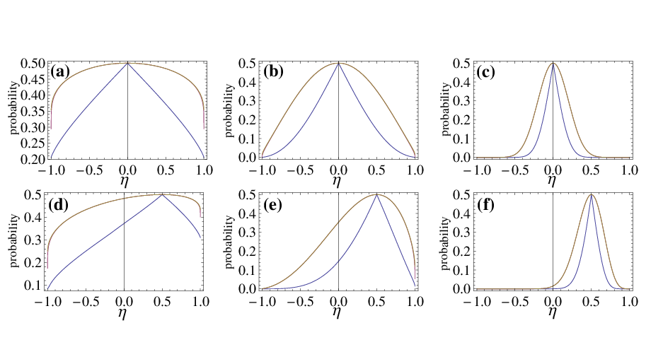
We now compute the QCB. The minimum error probability in the $n$-use adaptive discrimination of two arbitrary HW channels $\mathcal{W}_{\eta,d}$ and $\mathcal{W}_{\zeta,d}$ is bounded by the QCB as in Eqs. (26) and (27), where $Q:=Q(W_{\eta,d},W_{\zeta,d})$ is computed as the QCB between two corresponding Werner states $W_{\eta,d}$ and $W_{\zeta,d}$. We find

where the infimum is analytically achieved at

In fact, since we may diagonalise two Werner states in the same basis, Eq. (27) simplifies to $\sum_{i}p_{i}^{s}q_{i}^{1-s}$, with $p_{i},q_{i}$ the eigenvalues of $W_{\eta,d}$ and $W_{\zeta,d}$, respectively. We then minimise this quantity by finding the unique turning point in $[0,1]$ and showing it is indeed a minimum. The border points need a careful consideration because they may show discontinuities and one needs to take left or right limits. This is explicitly done in Appendix A. In Fig. 1, we show numerical examples on how the fidelity-based lower bound and the QCB [see Eq. (26)] behave in terms of $n$ for different values of the channel-defining parameters $\eta$ and $\zeta$ for arbitrary finite dimension $d\geq 2$.

Using the same approach, we may also find an equivalent result for depolarizing channels and their Choi matrices (isotropic states). The minimum error probability in the $n$-use adaptive discrimination of two arbitrary depolarizing channels $\mathcal{D}_{\alpha,d}$ and $\mathcal{D}_{\beta,d}$ is bounded by $p_{\text{err}}^{\text{opt}}\leq Q^{n}/2$ where $Q:=Q(\Omega_{\alpha,d},\Omega_{\beta,d})$ is computed as the QCB between two corresponding isotropic states $\Omega_{\alpha,d}$ and $\Omega_{\beta,d}$. We find

where the infimum is analytically achieved at

See Appendix B for mathematical details. This bound for two depolarizing channels is tighter than the fidelity-based upper bound of Ref. [33].

In this work, for the first time, we have considered Holevo-Werner channels in the context of quantum metrology and quantum channel discrimination, employing the most general (adaptive) protocols. Because these channels are teleportation-covariant, the optimal estimation of their channel-defining parameter $\eta$ is bounded by the standard quantum limit, with an asymptotically achievable scaling of $(1-\eta^{2})n^{-1}$. Surprisingly this scaling is independent of the dimension of the channel.

We have then investigated the multi-use optimal error probability in the adaptive discrimination of two iso-dimensional Holevo-Werner channels. By using their teleportation-covariance and the methodology introduced in Ref. [33], we have lower- and upper-bounded this optimal probability by means of single-letter quantities which can be analytically computed from the associated Werner states. In particular, we have given an explicit formula for the quantum Chernoff bound, with a similar counterpart for the case of depolarizing channels.

Acknowledgements. This work has been supported by the EPSRC via the ‘UK Quantum Communications Hub’ (EP/M013472/1). T.P.W.C. also acknowledges funding from a White Rose Scholarship.

References

- [1] M. A. Nielsen, and I. L. Chuang, Quantum Computation and Quantum Information (Cambridge University Press, Cambridge, 2000).
- [2] M. Hayashi, Quantum Information Theory: Mathematical Foundation (Springer-Verlag Berlin Heidelberg, 2017).
- [3] C. Weedbrook, S. Pirandola, R. García-Patrón, N. J. Cerf, T. C. Ralph, J. H. Shapiro, and S. Lloyd, Rev. Mod. Phys. 84, 621 (2012).
- [4] S. L. Braunstein and P. van Loock, Rev. Mod. Phys. 77, 513 (2005).
- [5] U. L. Andersen, J. S. Neergaard-Nielsen, P. van Loock, and A. Furusawa, Nature Phys. 11, 713 (2015).
- [6] H. J. Kimble, Nature 453, 1023 (2008).
- [7] S. Pirandola, and S. L. Braunstein, Nature 532, 169 (2016).
- [8] C. H. Bennett and G. Brassard. Quantum Cryptography: Public Key Distribution and Coin Tossing, Proceedings of IEEE International Conference on Computers, Systems and Signal Processing, 175 (1984).
- [9] A.K. Ekert, Phys. Rev. Lett. 67, 661 (1991).
- [10] N. Gisin, G. Ribordy, W. Tittel, and H. Zbinden, Rev. Mod. Phys. 74, 145 (2002).
- [11] F. Grosshans, G. Van Ache, J. Wenger, R. Brouri, N. J. Cerf, and P. Grangier, Nature 421, 238 (2003).
- [12] C. Weedbrook, A. M. Lance, W. P. Bowen, T. Symul, T. C. Ralph, and P. K. Lam, Phys. Rev. Lett. 93, 170504 (2004).
- [13] R. Colbeck, Quantum And Relativistic Protocols For Secure Multi-Party Computation (PhD thesis, University of Cambridge, 2006).
- [14] S. Pirandola, S. Mancini, S. Lloyd, and S. L. Braunstein, Nat. Phys. 4, 726 (2008).
- [15] S. L. Braunstein and S. Pirandola, Phys. Rev. Lett. 108, 130502 (2012).
- [16] M.Curty, B. Qi, H.K. Lo, Phys. Rev. Lett. 108, 130503 (2012).
- [17] S. Pirandola, C. Ottaviani, G. Spedalieri, C. Weedbrook, S. L. Braunstein, S. Lloyd, T. Ghering, C.S. Jacobsen, and U. L. Andersen, Nat. Photon. 9, 397 (2015).
- [18] E. Diamanti and A. Leverrier, Entropy 17, 6072 (2015).
- [19] V. C. Usenko and R. Filip, Entropy 18, 20 (2016).
- [20] P. Shor, Polynomial-Time Algorithms for Prime Factorization and Discrete Logarithms on a Quantum Computer, Proceedings of the 35th Annual Symposium on Foundations of Computer Science, Santa Fe (1994).
- [21] S. Lloyd and S. L. Braunstein, Phys. Rev. Lett. 82, 1784 (1999).
- [22] T. D. Ladd, F. Jelezko, R. Laflamme,Y. Nakamura, C. Monroe and J. L. O’Brien, Nature 464, 45 (2010).
- [23] S. L. Braunstein and C. M. Caves, Phys. Rev. Lett. 72, 3439 (1994).
- [24] P. Kok, S. L. Braunstein and J. P. Dowling, J. Op. B 6, 8 (2004).
- [25] V. Giovannetti, S. Lloyd and L. Maccone, Science 306, 1330 (2004).
- [26] H. M. Wiseman and G. J. Milburn, Quantum Measurement and Control (Cambridge University Press, 2010).
- [27] V. Giovannetti, S. Lloyd, and L. Maccone, Nature Photonics 5, 222–229 (2011).
- [28] G. Toth, I. Apellaniz, J. Phys. A: Math. Theor. 47, 424006 (2014).
- [29] M. G. A. Paris, Int. J. Quant. Inf. 7, 125 (2009).
- [30] M. Tsang, R. Nair, and X. Lu, Phys. Rev. X 6, 031033 (2016).
- [31] C. Lupo and S. Pirandola, Phys. Rev. Lett. 117, 190802 (2016).
- [32] R. Nair, and M. Tsang, Phys. Rev. Lett. 117, 190801 (2016).
- [33] S. Pirandola, and C. Lupo, Phys. Rev. Lett. 118, 100502 (2017); ibid. 119, 129901 (2017).
- [34] A. Chefles, Contemp. Phys. 41, 401 (2000).
- [35] S. M. Barnett and S. Croke, Advances in Optics and Photonics 1, 238 (2009).
- [36] C. Invernizzi, M. G. A. Paris, and S. Pirandola, Phys. Rev. A 84, 022334 (2011).
- [37] K. M. R. Audenaert, M. Nussbaum, A. Szkola, and F. Verstraete, Commun. Math. Phys. 279, 251 (2008).
- [38] G. Spedalieri and S. L. Braunstein, Phys. Rev. A 90, 052307 (2014).
- [39] S. Pirandola, Phys. Rev. Lett. 106, 090504 (2011).
- [40] S. Pirandola, C. Lupo, V. Giovannetti, S. Mancini, and S. L. Braunstein, New J. Phys. 13, 113012 (2011).
- [41] G. Spedalieri, C. Lupo, S. Mancini, S. L. Braunstein, and S. Pirandola, Phys. Rev. A 86, 012315 (2012).
- [42] C. Lupo, S. Pirandola, V. Giovannetti, and S. Mancini, Phys. Rev. A 87, 062310 (2013).
- [43] R. Nair, Phys. Rev. A 84, 032312 (2011).
- [44] O. Hirota, arXiv:1108.4163 (2011).
- [45] A. Bisio, M. Dall’Arno, and G. M. D’Ariano, Phys. Rev. A 84, 012310 (2011).
- [46] M. Dall’Arno et al., Phys. Rev. A 85, 012308 (2012).
- [47] S. Lloyd, Science 321, 1463 (2008).
- [48] S.-H. Tan et al., Phys. Rev. Lett. 101, 253601 (2008).
- [49] S. Barzanjeh et al., Phys. Rev. Lett. 114, 080503 (2015).
- [50] C. Weedbrook, S. Pirandola, J. Thompson, V. Vedral, and M. Gu, New J. Phys. 18, 043027 (2016).
- [51] E. D. Lopaeva, I. Ruo Berchera, I. P. Degiovanni, S. Olivares, G. Brida, and M. Genovese, Phys. Rev. Lett. 110, 153603 (2013).
- [52] Z. Zhang, S. Mouradian, F. N.C. Wong, and J. H. Shapiro, Phys. Rev. Lett. 114, 110506 (2015).
- [53] C. W. Helstrom, Quantum Detection and Estimation Theory (New York: Academic, 1976).
- [54] A. Uhlmann, Rep. Math. Phys. 9, 273 (1976).
- [55] R. Jozsa, Journal of Modern Optics 41, 2315 (1994).
- [56] L. Banchi, S. L. Braunstein, and S. Pirandola, Phys. Rev. Lett. 115, 260501 (2015).
- [57] K. M. R. Audenaert et al., Phys. Rev. Lett. 98, 160501 (2007).
- [58] J. Calsamiglia, R. Munoz-Tapia, L. Masanes, A. Acin, and E. Bagan, Phys. Rev. A 77, 032311 (2008).
- [59] S. Pirandola, and S. Lloyd, Phys. Rev. A 78, 012331 (2008).
- [60] C. H. Bennett, G. Brassard, C. Crepeau, R. Jozsa, A. Peres, and W. K. Wootters, Phys. Rev. Lett. 70, 1895 (1993).
- [61] S. L. Braunstein, and H. J. Kimble, Phys. Rev. Lett. 80, 869 (1998).
- [62] S. Pirandola, J. Eisert, C. Weedbrook, A. Furusawa, and S. L. Braunstein, Nat. Photon. 9, 641 (2015).
- [63] S. Pirandola, R. Laurenza, C. Ottaviani and L. Banchi, Nat. Comm. 8, 15043 (2017). See also arXiv:1510.08863 (2015).
- [64] S. Pirandola, S. L. Braunstein, R. Laurenza, C. Ottaviani, T. P. W. Cope, G. Spedalieri, and L. Banchi, Theory of Channel Simulation and Bounds for Private Communication, arXiv:1711.09909v1 (2017).
- [65] R. F. Werner, Phys. Rev. A, 40, 4277 (Oct 1989).
- [66] F. Barrett, Phys. Rev. A 65, 042302 (2002).
- [67] D. Z. Djokovic, Entropy 18, 216 (2016).
- [68] R. F. Werner, and A.S. Holevo, J. Mat. Phys. 43, 4353 (2002).
- [69] S. L. Braustein, and C. M. Caves, G. J. Milburn, Ann. Phys. 247, 135 (1996).
- [70] K. G. H. Vollbrecht and R. F. Werner, Phys. Rev. A 64, 062307 (2001).
- [71] V. Vedral, M. B. Plenio, M. A. Rippin, and P. L. Knight, Phys. Rev. Lett. 78, 2275 (1997).
- [72] V. Vedral, and M. B. Plenio, Phys. Rev. A 57, 1619 (1998).
- [73] V. Vedral, Rev. Mod. Phys. 74, 197 (2002).
- [74] M. Fannes, B. Haegeman,M. Mosonyi and D. Vanpeteghem, arXiv:quant-ph/0410195 (2004).
- [75] M. Horodecki and P. Horodecki, Phys. Rev. A 59, 4206 (1999).
- [76] A. Muller-Hermes, Transposition in Quantum Information Theory (Master’s thesis, Technical University of Munich, 2012).
- [77] M. M. Wolf, Notes on “Quantum Channels & Operations” (see page 35). Available at https://www-m5.ma.tum.de/foswiki/pub/M5/Allgemeines/ MichaelWolf/QChannelLecture.pdf.
- [78] D. Leung and W. Matthews, IEEE Trans. Info. Theory 61, 4486 (2015).
- [79] S. Pirandola, Capacities of Repeater-Assisted Quantum Communications, arXiv:1601.00966 (2016).
- [80] R. Laurenza and S. Pirandola, Phys. Rev. A 96, 032318 (2017).
- [81] R. Laurenza, S. L. Braunstein, and S. Pirandola, Finite-Resource Teleportation Stretching for Continuous-Variable Systems, arXiv:1706.06065 (2017).
- [82] T. P. W. Cope, L. Hetzel, L. Banchi, and S. Pirandola, Phys. Rev. A 96, 022323 (2017).
- [83] R. Laurenza, C. Lupo, G. Spedalieri, S. L. Braunstein, and S. Pirandola, Channel Simulation in Quantum Metrology, arXiv:1712.06603 (2017).
- [84] R. D. Gill and S. Massar, Phys. Rev. A 61, 042312 (2000).