Combinatorial Preconditioners for Proximal Algorithms on Graphs
Thomas Möllenhoff Zhenzhang Ye Tao Wu Daniel Cremers
Department of Informatics, Technical University of Munich, Germany {thomas.moellenhoff, zhenzhang.ye, tao.wu, cremers}tum.de
Abstract
We present a novel preconditioning technique for proximal optimization methods that relies on graph algorithms to construct effective preconditioners. Such combinatorial preconditioners arise from partitioning the graph into forests. We prove that certain decompositions lead to a theoretically optimal condition number. We also show how ideal decompositions can be realized using matroid partitioning and propose efficient greedy variants thereof for large-scale problems. Coupled with specialized solvers for the resulting scaled proximal subproblems, the preconditioned algorithm achieves competitive performance in machine learning and vision applications.
1 Introduction
Many applications in statistics [48], learning [27], and imaging [11] rely on efficiently solving convex-concave saddle-point problems:
| (1) |
Here the model is formulated on an undirected weighted graph , whose edges are weighted by a given function . The extended real-valued functions and are assumed to be proper, lower semi-continuous and convex. The notation refers to the convex conjugate of . The (linear) vertex-to-edge map is defined by
where is the (transposed) incidence matrix of , i.e.
with arbitrarily fixed orientation. For being the -norm, i.e. , this choice yields the total-variation semi-norm of functions on a weighted graph. In addition to its ubiquitous applications in image processing and computer vision, this semi-norm has recently gained considerable attention in unsupervised learning [27, 28, 8], semi-supervised learning [22], collaborative filtering [6], clustering [22] and statistical inference [52].
Among other proximal algorithms (see [41, 13] and the references therein for an overview), the primal-dual hybrid gradient (PDHG) algorithm [2, 55, 43, 19, 11] is a popular solver for the problem in (1). A general formulation of PDHG iterations [13] appears as follows:
| (2) | ||||
| (3) |
Here and are symmetric positive definite matrices, such that is a scaled norm defined by and analogously for . For given and , the convergence of PDHG is guaranteed if the (inverse) step sizes satisfy , cf. [42, Lemma 1]. Interestingly, as pointed out by [19, 11, 13], the formulation in (2)–(3) provides a flexible framework for deriving various types of proximal splitting algorithms, e.g. the proximal gradient method, Douglas-Rachford splitting, and (linearized) ADMM. Proximal algorithms in form of (2)–(3) are particularly efficient when , admit separable structures and , are diagonal. In this scenario, solutions of the subproblems in (2) and (3) refer to pointwise proximal evaluations. Nonetheless, many research efforts have been devoted to further accelerating the convergence speed.
To this end, two categories of acceleration strategies are envisaged: multi-step acceleration and preconditioning. Classical (optimal) multi-step gradient descent methods are attributed to [44, 38]. In the context of proximal algorithms, the FISTA algorithm [4] was proposed as an accelerated proximal gradient method, and in [12] a multi-step PDHG was devised.
On the other hand, a preconditioning technique aims to accelerate convergence, typically through reducing the number of outer iterations, by choosing proper scaling matrices and (also called the preconditioners in this context). In contrast to their counterparts for solving linear systems, preconditioning techniques for proximal algorithms are much less developed. Diagonal preconditioners for PDHG were explored in [42]; Preconditioners for other types of proximal algorithms [5, 23, 24, 35, 54, 7, 25, 20] also appeared recently in the literature.
A consensus among all existing preconditioning approaches appears that, while favorably reducing the number of outer iterations, preconditioning could explode the overall computational load by expensive inner proximal evaluations. For example, for proximal gradient method in minimizing a sum of smooth and nonsmooth functions, using the (approximate) Hessian of the smooth function as preconditioner may attain superlinear convergence in the outer iteration but also lead to very expensive proximal (or backward) steps; see [35]. This is the reason why diagonal preconditioners remain a popular choice in many recent works, and non-diagonal preconditioners designed in [5, 54, 21] do not deviate far from the diagonal ones.
In this work, we propose combinatorial preconditioners for proximal algorithms based on a partitioning of the original graph into forests. This leads to a class of block diagonal preconditioners, and the resulting PDHG updates refer to solving parallel subproblems on forests. We show how to construct such preconditioners guided by theoretical estimates of the condition number. Coupled with fast direct solvers for proximal evaluation on forests, we achieve significant performance boost for the PDHG algorithm across a series of numerical tests.
2 Preconditioner and Condition Number
The choice of and can significantly influence the convergence speed of the (generalized) PDHG scheme, (2)–(3), in practice. In [42], Pock and Chambolle showed that utilization of diagonal preconditioners and yields a visible performance boost in comparison with PDHG without preconditioning (i.e. ). In a slightly different context, Boyd et al. [16, 20, 23, 24, 25] also considered diagonal preconditioning strategies for other closely related proximal algorithms. In particular, they suggested based on extensive numerical experiments that an ideal choice of and ought to minimize the (finite) condition number defined by
| (4) |
i.e. the ratio between largest and smallest non-zero singular value. This rule of thumb was computationally pursued by so called matrix equilibration [16, 25, 1].
A more quantified connection between the convergence rate of (2)–(3) and can be drawn in a more specific setting, e.g. for some given . By choosing in (2)–(3), one comes up with the following proximal gradient iteration:
| (5) |
When is the indicator function of a polyhedral set it can be shown that iteration (5) converges linearly [37]. More precisely, with step size choice the linear convergence rate can be derived (cf. [37, Theorem 11]) as:
where denotes Hoffman’s bound [29, 50]. In the extreme case where (e.g., for strong regularizations), Hoffman’s bound reduces to and matches the condition number .
3 Combinatorial Preconditioners
Following the discussion in the previous section, reducing provides a reasonable guideline for the choice of preconditioners. As is the weighted incidence matrix of , this boils down to constructing “good” approximations of the graph. Meanwhile, as discussed in the introduction, the non-diagonal or could possibly explode the computational cost of the proximal evaluation in (2)–(3). Hence, an ideal choice of preconditioners would strike a balance between reduced (outer) iteration number and costlier proximal evaluations per iteration.
Bearing this in mind, in this section we propose our combinatorial preconditioners based on graph partitioning. This leads to a family of block diagonal preconditioners for . For simplicity we fix in our development, and remark that can be adapted to work properly with any diagonal preconditioner (e.g. the one used in [42]). In terms of the update scheme (3), such preconditioning yields proximal evaluation on respective partitioned subgraphs, which can be efficiently carried out by using the state-of-the-art direct solver on trees [34].
As a remark, there is a connection between our combinatorial preconditioners and the subgraph preconditioners for solving linear systems in graph Laplacians; see, e.g., [46] and the references therein. Pioneered by Vaidya and his coworkers in the early 1990s [49, 32], a series of works are done in finding a subgraph preconditioner. An ideal subgraph preconditioner uses a graph Laplacian on some (low-stretch) spanning tree which best preserves connectivity between vertices in the original graph. In some sense, our proposed combinatorial preconditioners are dual analogues of the subgraph preconditioners.
In Section 3.1, we show how to construct via graph partitioning and under which sufficient conditions the condition number can be (optimally) reduced. In Section 3.2, such sufficient conditions are algorithmically realized by: (1) chains on regular grid; (2) nested forests on general graph. In Section 3.3, we detail the message passing based implementation of efficient proximal evaluation on forests.
3.1 Preconditioning via Graph Partitioning
Let the edge set be partitioned into mutually disjoint subsets, i.e. , such that each subgraph is a forest, i.e. has no cycle. Correspondingly, we define as the canonical projection from to , i.e. for each . Thus, the matrix can be decomposed into submatrices where each . Analogously let and . Note that each has full column rank.
We then define our preconditioners as follows
It follows from (4) that
| (6) |
| (7) |
Indeed, each is the orthogonal projection onto the subspace , and hence and . It follows immediately from (7) that
| (8) |
and therefore it suffices for the sake of convergence to choose step sizes such that .
In the remainder of Section 3.1, we show analytically how certain graph partitions can attain optimal condition number in a two-partition scenario, i.e. . The two-partition scenario is motivated from many applications where is a 2D regular grid (whose maximum degree equals 4). In this case, it is guaranteed by Nash-Williams’ theorem [36] that can be covered by two disjoint forests. Our theory suggests that either a chain decomposition or a nested-forest decomposition makes a good preconditioner on the 2D regular grid. Furthermore, the nested-forest preconditioners further extend to any general weighted graph, with aid of either the matroid partition algorithm [18] or some greedy algorithm; see Section 3.2.2.
The following theorem derives a lower bound for for a wide range of two-partition cases. We denote by the column rank of . In terms of graph theory, identifies the maximum number of the edges in that are cycle-free. is understood as the Moore-Penrose pseudoinverse when is singular. The two assumptions rule out pathological cases where is either too sparse (e.g. cycle-free) or too dense (e.g. fully connected). In the proof, we shall use Weyl’s inequality [51]:
| (9) |
where , , and denotes the -th largest eigenvalue of a real symmetric matrix.
Theorem 1.
Let be partitioned into two nonempty subgraphs and (not necessarily forests) such that
- 1.
- 2.
Then we have .
Proof.
By Weyl’s inequality (9), we have . Moreover, condition 1 ensures that there exists some nonzero with . Hence, we must have .
We proceed to propose sufficient conditions for graph partitioning (in particular when ) which guarantee optimal condition number .
Theorem 2.
Let be partitioned into two forests and . If the following conditions are satisfied
- 1.
,
- 2.
,
- 3.
,
then .
Proof.
The proof of is identical to that for Theorem 1.
On the other hand, we have
where by commutativity (i.e. condition 1)
Note that is an orthogonal projection onto , and hence for all . Meanwhile, condition 2 asserts that and for some . Altogether, and the conclusion follows. ∎
Theorem 3.
Let be partitioned into (nonempty) nested forests, namely , in the sense that
Then we have .
Proof.
Recall (8) that . Indeed, we have since for any nonzero . On the other hand, note that . Therefore, for all , we have and the equality holds when . This gives , which concludes the proof. ∎
3.2 Two Classes of Forest Preconditioners
 |
 |
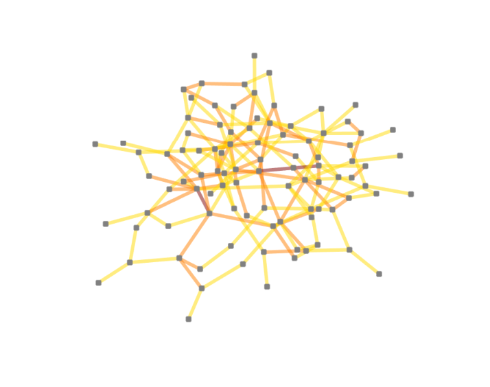 |
 |
| No preconditioning | Greedy linear forests | Greedy nested forests | Matroid partitioning |
Given the abstract conditions from Theorem 2 and 3 under which graph partitioning achieves optimal condition number, the question remains whether such partitions exist and how they can be constructed in practice. In the following section we propose optimal partitioning approaches, depending on the topology of the underlying graph. We first focus on regular grid graphs, which are ubiquitous in signal processing and computer vision applications.
3.2.1 Chains on Regular Grid
Formally, -dimensional grid graphs are given as the -fold Cartesian product between path graphs , . For ease of presentation we will focus mostly on two dimensional grids. Recall that the Cartesian product yields a graph with vertex set . In that graph, two vertices and are adjacent if and only if and is adjacent to or and is adjacent to . Whether a given graph is a grid graph can be tested in linear time [30]. The procedure described in [30] yields a natural decomposition of the -dimensional grid into linear forests, i.e., a forest in which every tree is a path graph. Moreover, in the aforementioned decomposition, each forest consists of paths of equal length. To be precise, in the case the decomposition is given by
| (10) |
where . We refer to the connected components of as horizontal chains and as vertical chains. Such a natural splitting into chains enjoys a theoretically optimal condition number among the large class of decompositions characterized by Theorem 1.
Theorem 4.
Let be a regular grid of dimension (). The condition number in the unpreconditioned case is bounded by
| (11) |
The natural partitioning of into two linear forests (10) achieves condition number
| (12) |
Proof.
The bound (11) follows from elementary results in spectral graph theory. The spectrum of a path graph of dimension is , , see [9, Section 1.4.4]. The spectrum of the Cartesian product graph is given by the summing all pairs of eigenvalues of the individual graphs, cf. [9, Section 1.4.6]. Using the inequality we have
To show (12) it suffices to verify the three conditions in Theorem 2. Denoting by the ones-vector and by the Kronecker product, the projections are explicitly given by
Since , the condition from Theorem 2 follows directly.
Now note that each projection subtracts the mean on the chains it contains. Conditions 2 and 3 can be verified by counting dimensions. For condition 2, simply pick nonzero to be constant along chains in but non-constant along chains in . For condition 3, pick nonzero that is zero-mean on the chains in both and . ∎
We remark that the above results can be generalized to the -dimensional setting, yielding and . Remarkably the chains preconditioning mentioned above makes the condition number independent of the grid size, while for the unpreconditioned case, it exhibits linear growth with respect to the largest grid dimension.
Furthermore, the splitting into chains leads to a particularly efficient evaluation of the dual subproblem in PDHG as we will see later on. Together with the theoretically optimal condition number, this makes the chains the number one choice of preconditioner for the regular -dimensional grid.
3.2.2 Nested Forests on General Graphs
Matroid partitioning.
The situation on general graphs is more involved than on grid graphs. Inspired by Theorem 3, we seek to partition into nested forests such that the number of forests is minimal, i.e. equal to the arboricity of the graph [36]. If is connected, the arboricity of can be calculated as: .
It turns out that the classical matroid partitioning algorithm by Edmonds [18] meets our requirements. In short, matroid partitioning progressively inserts an idle edge into the forest partitions. To preserve all partitions cycle-free, it relies on a primitive operation which detects a simple cycle (also called circuit) whenever this occurs due to the insertion of a new edge into a forest. By the nature of the algorithm, the resulting partitions are guaranteed to be (a minimal number of) nested forests, and hence realize the condition posed in Theorem 3.
| Nested Forest | ||||||||
| No Precond. | Linear Forest | Greedy | Matroid | |||||
| it | it | it | it | |||||
| 0.68 | 53.8 | 1624 | 24.9 | 789 | 1 | 36 | 1 | 36 |
| 1.11 | 257.0 | 6245 | 148.7 | 3782 | 2 | 80 | 2 | 80 |
| 2.36 | 82.2 | 2061 | 14.1 | 577 | 4 | 143 | 3 | 103 |
| 2.98 | 27.7 | 1010 | 12.4 | 484 | 5 | 194 | 4 | 137 |
| 4.25 | 24.9 | 800 | 10.1 | 419 | 7 | 254 | 5 | 166 |
| 6.48 | 7.7 | 367 | 5.6 | 176 | 10 | 362 | 1.75 | 59 |
In spite of such favorable properties of matroid partitioning, its complexity grows like , cf. [33], making its application prohibitive for large graphs.
Greedy nested forests.
As a remedy, we propose the following “greedy nested forests” heuristic: given the input graph we successively subtract a spanning forest until no edges remain. The individual subtracted forests form the graph partitioning . While this greedy approach does not guarantee a minimal number of forests , the partition still satisfies the assumption of Theorem 3. Indeed, each edge in the forest can be represented by a path in since adding that edge from to would form a cycle due to the spanning forest property.
Greedy linear forests.
Since the dual update can be computed very efficiently for linear forests we modify the above procedure to yield a linear forest decomposition. Before subtracting the spanning forest from the residual graph, we remove all edges which contain a vertex with degree larger than 2. In addition, we check whether it is possible to add any edges from the residual graph to the current linear forest without turning it into a general forest.
In Table 1 we show the condition number for the different partitioning strategies on small random Erdős-Renyi graphs of varying average degree. While the matroid partitioning strategy finds the lowest condition number, both greedy heuristics also lead to a reduction in condition number for most cases. The greedy nested forest heuristic works best for graphs with low edge-to-vertex ratio, while the linear forest heuristic is preferable for dense graphs.
3.3 Proximal Evaluation on Forests
In this section we will discuss how the dual update (3) is computed for our combinatorial preconditioner . Assuming that is separable across the subgraphs ,
the dual update (3) decomposes into parallel problems:
| (13) |
Let us now further assume that the individual are forests and .
Expanding the norm and completing the square in (13) leads to the problem
| (14) |
with . The dual problem to (14) is given by
| (15) |
This further parallelizes into weighted total variation problems on the individual trees in the forest . These problems can be handled due to recent advances in direct total-variation solvers; see [15, 17, 31, 14, 3, 34]. The original taut-string algorithm [15, 17] solves the 1D total-variation problem in iterations on a chain. Condat [14] proposed an algorithm which has worst-case complexity but it achieves good performance in practice. Barbero and Sra [3] proposed a generalization of the taut-string approach to the case of weighted total variation which runs in . The approach proposed by Johnson [31] also runs in time, works for weighted total variation and has good practical performance. Furthermore, a more memory efficient implementation of Johnson’s algorithm generalization to trees was proposed by Kolmogorov et al. [34] – which appears to be state-of-the-art.
We use our implementation of the algorithm proposed by Kolmogorov et al. [34] to find the exact minimizer on each tree. The algorithm computes derivatives of messages and for and in the order from leaves toward the root, which are defined as the following:
The derivatives are denoted as , and . The procedure is summarized in Algorithm 1.
| Instance | None [11] | Diagonal [42] | Nested Forest | Linear Forest | ||||||
| name | it | time[s] | it | time[s] | it | time[s] | it | time[s] | ||
| synthetic | ||||||||||
| rmf-long.n2 | 64 | 2.87 | – | – | – | – | 1794 | 62.9 (+0.7) | 5070 | 24.4 (+1.2) |
| rmf-wide.n2 | 32 | 2.84 | – | – | – | – | 159 | 2.6 (+0.3) | 23518 | 62.2 (+0.6) |
| wash-rlg-long.n1024 | 64 | 2.99 | 73309 | 134.1 (+9.4) | 14333 | 49.7 (+0.0) | 5848 | 373.9 (+0.8) | 18798 | 108.7 (+1.3) |
| bisection | ||||||||||
| horse-48112 | 47 | 2.99 | – | – | 21593 | 38.3 (+0.0) | 964 | 33.9 (+0.3) | 19145 | 90.4 (+2.8) |
| alue7065-33338 | 33 | 1.61 | – | – | 23218 | 21.5 (+0.0) | 2499 | 21.4 (+0.17) | 49452 | 99.4 (+1.7) |
| stereo | ||||||||||
| BVZ-venus1* | 162 | 1.99 | 9068 | 20.8 (+7.9) | 3741 | 20.2 (+0.0) | 1111 | 90.7 (+0.9) | 414 | 1.9 (+0.1) |
| BVZ-venus2* | 162 | 1.99 | 10099 | 24.4 (+7.9) | 3124 | 17.2 (+0.0) | 1065 | 88.8 (+0.9) | 384 | 1.7 (+0.1) |
| KZ2-sawtooth1 | 310 | 2.91 | 96974 | 736.5 (+31.8) | 3468 | 51.7 (+0.0) | 336 | 102.8 (+3.0) | 526 | 14.9 (+6.1) |
| KZ2-sawtooth2 | 294 | 2.79 | 95849 | 675.3 (+33.1) | 3520 | 48.2 (+0.0) | 432 | 124.8 (+2.9) | 652 | 15.7 (+5.8) |
| misc vision | ||||||||||
| texture_graph | 9 | 4.76 | 4860 | 1.6 (+1.45) | 3554 | 1.9 (+0.0) | 1091 | 9.12 (+0.1) | 1669 | 1.7 (+0.3) |
| lazybrush-mangagirl* | 579 | 1.99 | – | – | – | – | 13318 | 5727.3 (+3.3) | 6330 | 95.4 (+0.4) |
| imgseggmm-ferro | 231 | 3.98 | 3594 | 32.2 (+75.9) | 5806 | 95.0 (+0.0) | 786 | 276.8 (+4.4) | 775 | 25.6 (+3.1) |
After running Algorithm 1 for each forest , the solution to (14) is given by the optimality condition
Since each is a forest, the corresponding matrix has full column rank which implies that the linear system has a unique solution. Rows of corresponding to leaf nodes in the tree contain exactly one nonzero element. Therefore, we solve the linear equation by starting from leaves toward the root. Consistency on the branch nodes is guaranteed due to the uniqueness of the solution. Even though we only discussed the case of total variation , we remark that for various other choices of (e.g., Huber penalty) efficient solvers on trees are conceivable.
4 Numerical Validation
The preconditioned PDHG algorithm (2)–(3) for total variation minimization on weighted graphs is summarized in Algorithm 2. We assume that the primal update can be efficiently computed, e.g. if is separable.
For the experiments we compare the proposed preconditioners to the unpreconditioned variant of PDHG (, , , ), the diagonal preconditioners from [42] with choice of and . When using the proposed preconditioners we employ the balanced step size choice , .
We implemented all algorithms in MATLAB, whereas time critical parts such as the total variation solver on a tree (Algorithm 1) were implemented in C++.
4.1 Generalized Fused Lasso
The fused lasso [48], also known as the Rudin-Osher-Fatemi (ROF) model [45] to the image processing community is readily generalized to graphs:
| (16) |
Despite its simplicity, this model has a plethora of applications in statistics [52], machine learning [27, 8] and computer vision [47, 39], often as a subproblem in sequential convex programming for nonconvex minimization.
We solve (16) using the accelerated PDHG variant ([11, Algorithm 2], ) since the energy (16) is -strongly convex. In Table 1 we compare the number of iterations required to solve (16) on small random graphs. We stop the algorithm once the relative primal-dual gap drops below . It can be observed that there is a clear correlation between the condition number and the number of required iterations, validating the discussion from Section 2. The optimal preconditioning based on matroid partitioning performs best.
We further validate our preconditioner on the maximum flow benchmark [26]11 1 http://www.cs.tau.ac.il/~sagihed/ibfs/. It is well known (cf. [10, 42]) that the minimum cut in a flow network can be obtained by thresholding the minimizing argument of (16). We remark that graph cuts can be efficiently found by highly specialized combinatorial solvers such as that in [26]. The point of this experiment is, however, to compare different preconditioners for continuous first-order algorithms on challenging real-world graphs.
In Table 2, we show iterations and run time for the proposed forest preconditioners, the unpreconditioned PDHG algorithm and the diagonal preconditioners [42]. Due to the size of the graphs, matroid partitioning is intractable, and we resort to the greedy nested forest and linear forest approaches. Combinatorial preconditioning consistently leads to a significant decrease in iterations. In all except one case, the overall lowest run time is achieved either by linear forest decomposition or greedy nested forest decomposition.
Despite the huge decrease in the total number of outer iterations for the nested forest preconditioning, in some cases, the overall run time is worse than without preconditioning. This motivates the construction of preconditioners like the greedy linear forests. These are clearly suboptimal with respect to condition number, but yield a good balance between efficient resolution of the backward step and the number of outer iterations. The chains on regular grid achieve the best of both worlds and lead to an improvement in runtime of an order of magnitude.
4.2 Multiclass Segmentation
 |
 |
| Input () + Scribbles | Result ( PDHG iterations) |
As a second example, we consider the multiclass total variation segmentation problem
under entropic regularization . is the indicator function of the -dimensional unit simplex .
The above model has various important applications in vision [53, 40] and transductive learning [22]. As the entropy term renders the objective ()-strongly convex we can again use the accelerated PDHG algorithm ([11, Algorithm 2] with ). We set for all experiments. Note that the model fits the general saddle point problem (1) under the choice , . To compute the proximal subproblem in (2) we first observe that .
Thanks to Moreau’s identity we reduce (2) to the proximal evaluation of , for which a few Newton iterations suffice. In Table 3 we compare the performance of our combinatorial preconditioners on two of the aforementioned applications. For the transductive learning scenario, we follow the procedure described in [22] to generate a -nearest neighbour graph () on the synthetic “three moons” data set. As in [22], the data term specifies the correct labels for of the points. We report a similar final accuracy () as the authors of [22]. As seen in Table 3, the nested forest preconditioning performs best.
For the second application, we consider interactive image segmentation [40]. Following that paper, we compute the data term from user scribbles (see Fig. 2). The weights are chosen based on the input image as
This essentially encourages the segmentation boundary to coincide with image discontinuities. We use a fixed scale parameter in all experiments. The performance of the different preconditioning strategies is shown in Table 3. Due to the underlying grid topology the natural linear forest decomposition into chains can be employed, which outperforms the other preconditioners and PDHG without preconditioning by an order of magnitude. While the nested forest preconditioner is competitive w.r.t. iterations, the proximal subproblem on the large spanning tree is very expensive. In contrast, the subproblem on the short chains can be computed efficiently.
| None [11] | Diag. [42] | Nest. Forest | Lin. Forest | |
| name | it (time[s]) | it (time[s]) | it (time[s]) | it (time[s]) |
| 3MOONS | 333 (2.8) | 474 (8.2) | 88 (1.1) | 303 (3.1) |
| icgbench-1* | 113 (47.0) | 131 (41.3) | 52 (41.9) | 13 (3.1) |
| icgbench-2* | 124 (54.7) | 159 (54.1) | 58 (47.9) | 11 (2.6) |
| icgbench-3* | 78 (29.1) | 95 (25.9) | 42 (27.2) | 9 (1.6) |
5 Conclusion
We proposed a novel combinatorial preconditioner for proximal algorithms on weighted graphs. The preconditioner is driven by a disjoint decomposition of the edge set into forests. Our theoretical analysis provides conditions under which such a decomposition achieves an optimal condition number. Furthermore, we have shown how provably optimal preconditioners can be obtained: on two-dimensional regular grids by a splitting into horizontal and vertical chains, on general graphs by means of matroid partitioning. We additionally proposed two fast heuristics to construct reasonable preconditioners on large scale graphs. We demonstrated how the resulting scaled proximal evaluations can be carried out by means of an efficient message passing algorithm on trees. In an extensive numerical evaluation we confirmed practical gains of preconditioning in terms of overall runtime as well as outer iteration numbers.
Acknowledgements
We thank Thomas Windheuser for fruitful discussions on combinatorial preconditioning. We gratefully acknowledge the support of the ERC Consolidator Grant 3D Reloaded.
References
- [1] Z. Allen-Zhu, Y. Li, R. Oliveira, and A. Wigderson. Much faster algorithms for matrix scaling. In Proceedings of the 58th IEEE Annual Symposium on Foundations of Computer Science, FOCS, 2017.
- [2] K. J. Arrow, L. Hurwicz, and H. Uzawa. Studies in Linear and Nonlinear Programming. Stanford University Press, 1958.
- [3] A. Barbero and S. Sra. Modular proximal optimization for multidimensional total-variation regularization. arXiv:1411.0589, 2014.
- [4] A. Beck and M. Teboulle. A fast iterative shrinkage-thresholding algorithm for linear inverse problems. SIAM J. Imaging Sci., 2:183–202, 2009.
- [5] S. Becker and M. J. Fadili. A quasi-Newton proximal splitting method. In Proceedings of the 26th International Conference on Neural Information Processing Systems, NIPS, 2012.
- [6] K. Benzi, V. Kalofolias, X. Bresson, and P. Vandergheynst. Song recommendation with non-negative matrix factorization and graph total variation. In Proceedings of the 42nd IEEE International Conference on Acoustics, Speech and Signal Processing, ICASSP, 2016.
- [7] K. Bredies and H. Sun. Preconditioned Douglas–Rachford splitting methods for convex-concave saddle-point problems. SIAM J. Numer. Anal., 53:421–444, 2015.
- [8] X. Bresson, T. Laurent, D. Uminsky, and J. Von Brecht. Multiclass total variation clustering. In Proceedings of the 27th International Conference on Neural Information Processing Systems, NIPS, 2013.
- [9] A. E. Brouwer and W. H. Haemers. Spectra of Graphs. Springer, 2012.
- [10] A. Chambolle and J. Darbon. On total variation minimization and surface evolution using parametric maximum flows. Int. J. Comput. Vis., 84:288–307, 2009.
- [11] A. Chambolle and T. Pock. A first-order primal-dual algorithm for convex problems with applications to imaging. J. Math. Imaging Vis., 40:120–145, 2011.
- [12] A. Chambolle and T. Pock. On the ergodic convergence rates of a first-order primal–dual algorithm. Math. Program., 159:253–287, 2016a.
- [13] A. Chambolle and T. Pock. An introduction to continuous optimization for imaging. Acta Numer., 25:161–319, 2016b.
- [14] L. Condat. A direct algorithm for 1D total variation denoising. IEEE Signal Process. Lett., 20:1054–1057, 2013.
- [15] P. L. Davies and A. Kovac. Local extremes, runs, strings and multiresolution. Ann. Stat., 29:1–48, 2001.
- [16] S. Diamond and S. Boyd. Stochastic matrix-free equilibration. J. Optim. Theory Appl., 172:436–454, 2017.
- [17] L. Dümbgen and A. Kovac. Extensions of smoothing via taut strings. Electron. J. Stat., 3:41–75, 2009.
- [18] J. Edmonds. Minimum partition of a matroid into independent subsets. J. Res. Natl. Bur. Standards, 69B:67–72, 1965.
- [19] E. Esser, X. Zhang, and T. F. Chan. A general framework for a class of first order primal-dual algorithms for convex optimization in imaging science. SIAM J. Imaging Sci., 3:1015–1046, 2010.
- [20] C. Fougner and S. Boyd. Parameter selection and pre-conditioning for a graph form solver. arXiv:1503.08366, 2015.
- [21] M. P. Friedlander and G. Goh. Efficient evaluation of scaled proximal operators. Electron. Trans. Numer. Anal., 46:1–22, 2017.
- [22] C. Garcia-Cardona, E. Merkurjev, A. L. Bertozzi, A. Flenner, and A. G. Percus. Multiclass data segmentation using diffuse interface methods on graphs. IEEE Trans. Pattern Anal. Mach. Intell., 36(8):1600–1613, 2014.
- [23] P. Giselsson and S. Boyd. Diagonal scaling in Douglas-Rachford splitting and ADMM. In Proceedings of the 53rd IEEE Conference on Decision and Control, CDC, 2014a.
- [24] P. Giselsson and S. Boyd. Preconditioning in fast dual gradient methods. In Proceedings of the 53rd IEEE Conference on Decision and Control, CDC, 2014b.
- [25] P. Giselsson and S. Boyd. Metric selection in fast dual forward–backward splitting. Automatica, 62:1–10, 2015.
- [26] A. Goldberg, S. Hed, H. Kaplan, R. Tarjan, and R. Werneck. Maximum flows by incremental breadth-first search. European Symposium on Algorithms, ALGO ESA, 2011.
- [27] M. Hein and S. Setzer. Beyond spectral clustering – tight relaxations of balanced graph cuts. In Proceedings of the 25th International Conference on Neural Information Processing Systems, NIPS, 2011.
- [28] M. Hein, S. Setzer, L. Jost, and S. S. Rangapuram. The total variation on hypergraphs – learning on hypergraphs revisited. In Proceedings of the 27th International Conference on Neural Information Processing Systems, NIPS, 2013.
- [29] A. J. Hoffman. On approximate solutions of systems of linear inequalities. J. Res. Natl. Bur. Standards, 49:263–265, 1952.
- [30] W. Imrich and I. Peterin. Recognizing Cartesian products in linear time. Discrete Math., 307:472–483, 2007.
- [31] N. A. Johnson. A dynamic programming algorithm for the fused lasso and -segmentation. J. Comput. Graph. Stat., 22(2):246–260, 2013.
- [32] A. Joshi. Topics in Optimization and Sparse Linear Systems. PhD thesis, UIUC, 1997.
- [33] D. E. Knuth. Matroid partitioning. Technical report, Stanford University, 1973.
- [34] V. Kolmogorov, T. Pock, and M. Rolinek. Total variation on a tree. SIAM J. Imaging Sci., 9:605–636, 2016.
- [35] J. D. Lee, Y. Sun, and M. A. Saunders. Proximal Newton-type methods for minimizing composite functions. SIAM J. Optim., 24:1420–1443, 2014.
- [36] C. S. A. Nash-Williams. Decomposition of finite graphs into forests. J. London Math. Soc., 39:12–12, 1964.
- [37] I. Necoara, Y. Nesterov, and F. Glineur. Linear convergence of first order methods for non-strongly convex optimization. arXiv:1504.06298, 2015.
- [38] Y. Nesterov. A method for solving the convex programming problem with convergence rate . Soviet Mathematics Doklady, 269:543–547, 1983.
- [39] R. A. Newcombe, S. J. Lovegrove, and A. J. Davison. DTAM: Dense tracking and mapping in real-time. In Proceedings of the 13th International Conference on Computer Vision, ICCV, 2011.
- [40] C. Nieuwenhuis and D. Cremers. Spatially varying color distributions for interactive multilabel segmentation. IEEE Trans. Pattern Anal. Mach. Intell., 35(5):1234–1247, 2013.
- [41] N. Parikh and S. Boyd. Proximal algorithms. Foundations and Trends in Optimization, 1:123–231, 2013.
- [42] T. Pock and A. Chambolle. Diagonal preconditioning for first order primal-dual algorithms in convex optimization. In Proceedings of the 13th International Conference on Computer Vision, ICCV, 2011.
- [43] T. Pock, D. Cremers, H. Bischof, and A. Chambolle. An algorithm for minimizing the piecewise smooth Mumford-Shah functional. In Proceedings of the 11th International Conference on Computer Vision, ICCV, 2009.
- [44] B. T. Polyak. Some methods of speeding up the convergence of iteration methods. USSR Computational Mathematics and Mathematical Physics, 4:1–17, 1964.
- [45] L. I. Rudin, S. Osher, and E. Fatemi. Nonlinear total variation based noise removal algorithms. Physica D: Nonlinear Phenomena, 60(1):259–268, 1992.
- [46] D. A. Spielman. Algorithms, graph theory, and linear equations in Laplacian matrices. In Proceedings of the International Congress of Mathematicians, ICM, 2010.
- [47] J. Stühmer, S. Gumhold, and D. Cremers. Real-time dense geometry from a handheld camera. In Proceedings of the 32nd DAGM Symposium on Pattern Recognition, 2010.
- [48] R. Tibshirani, M. Saunders, S. Rosset, J. Zhu, and K. Knight. Sparsity and smoothness via the fused lasso. J. R. Stat. Soc., 67(1):91–108, 2005.
- [49] P. M. Vaidya. Solving linear equations with symmetric diagonally dominant matrices by constructing good preconditioners. (A talk based on the manuscript was presented at the IMA Workshop on Graph Theory and Sparse Matrix Computation), 1991.
- [50] P.-W. Wang and C.-J. Lin. Iteration complexity of feasible descent methods for convex optimization. J. Mach. Learn. Res., 15:1523–1548, 2014.
- [51] H. Weyl. Das asymptotische Verteilungsgesetz der Eigenwerte linearer partieller Differentialgleichungen (mit einer Anwendung auf die Theorie der Hohlraumstrahlung). Mathematische Annalen, 71:441–479, 1912.
- [52] B. Xin, Y. Kawahara, Y. Wang, and W. Gao. Efficient generalized fused Lasso and its application to the diagnosis of Alzheimer’s disease. In Proceedings of the 28th AAAI Conference on Artificial Intelligence, 2014.
- [53] C. Zach, D. Gallup, J.-M. Frahm, and M. Niethammer. Fast global labeling for real-time stereo using multiple plane sweeps. In Proceedings of the Vision, Modeling and Visualization Workshop, 2008.
- [54] K. Zhong, I. E. H. Yen, I. S. Dhillon, and P. Ravikumar. Proximal quasi-Newton for computationally intensive -regularized -estimators. In Proceedings of the 28th International Conference on Neural Information Processing Systems, NIPS, 2014.
- [55] M. Zhu and T. F. Chan. An efficient primal-dual hybrid gradient algorithm for total variation image restoration. CAM Reports 08-34, UCLA, 2008.