跳到论文正文
W Papers独立论文阅读器 arXiv:1801.05268 论文正文 计算阅读时间 · 0%
引用这篇论文根据当前论文元数据生成,正式投稿前建议核对。


License: arXiv.org perpetual non-exclusive license
arXiv:1801.05268v2 [hep-ph] 12 Mar 2018

HUPD1714 Effective theory analysis for vector-like quark model

Takuya Morozumi1,2,  Yusuke Shimizu1,,

 Shunya Takahashi1,, and  Hiroyuki Umeeda3,

1Graduate School of Science, Hiroshima University,
Higashi-Hiroshima 739-8526, Japan
2Core of Research for the Energetic Universe, Hiroshima University,
Higashi-Hiroshima 739-8526, Japan
3Graduate School of Science and Engineering, Shimane University,
Matsue 690-8504, Japan
Note: E-mail address: morozumi@hiroshima-u.ac.jp Note: E-mail address: yu-shimizu@hiroshima-u.ac.jp Note: E-mail address: s-takahashi@hiroshima-u.ac.jp Note: E-mail address: umeeda@riko.shimane-u.ac.jp
Abstract
We study a model with a down-type SU(2) singlet vector-like quark (VLQ) as a minimal extension of the standard model (SM). In this model, flavor changing neutral currents (FCNCs) arise at tree level and the unitarity of the 3×33\times 3 Cabibbo-Kobayashi-Maskawa (CKM) matrix does not hold. In this paper, we constrain the FCNC coupling from b→sb\rightarrow s transitions, especially Bs→μ+​μ−B_{s}\rightarrow\mu^{+}\mu^{-} and B¯→Xs​γ\bar{B}\rightarrow X_{s}\gamma processes. In order to analyze these processes, we derive an effective Lagrangian which is valid below the electroweak symmetry breaking scale. For this purpose, we first integrate out the VLQ field and derive an effective theory by matching Wilson coefficients up to one-loop level. Using the effective theory, we construct the effective Lagrangian for b→s​γ(∗)b\rightarrow s\gamma^{(*)}. It includes the effects of the SM quarks and the violation of the CKM unitarity. We show the constraints on the magnitude of the FCNC coupling and its phase by taking account of the current experimental data on Δ​MBs\Delta M_{B_{s}}, Br[Bs→μ+μ−]\mathrm{Br}[B_{s}\rightarrow\mu^{+}\mu^{-}], Br[B¯→Xsγ]\mathrm{Br}[\bar{B}\rightarrow X_{s}\gamma] and CKM matrix elements as well as theoretical uncertainties. We find that the constraint from the Br[Bs→μ+μ−]\mathrm{Br}[B_{s}\rightarrow\mu^{+}\mu^{-}] is more stringent than that from the Br[B¯→Xsγ\mathrm{Br}[\bar{B}\rightarrow X_{s}\gamma]. We also obtain the bound for the mass of the VLQ and the strength of the Yukawa couplings related to the FCNC coupling of b→sb\rightarrow s transition. Using the CKM elements which satisfy above constraints, we show how the unitarity is violated on the complex plane.

1 Introduction

After the discovery of the Glashow-Iliopoulos-Maiani (GIM) mechanism [1], this suppression mechanism of the flavor changing neutral current (FCNC) is firmly verified in KK, DD and BB meson systems. The unitarity of the Cabibbo-Kobayashi-Maskawa (CKM) matrix [2] is also verified. As investigated in Refs. [3, 4], the CKM unitarity is consistent with current data, which characterizes one of the most successful aspects in the standard model (SM).

As an extension of the quark sector, vector-like quark (VLQ) is considered. Here, VLQ is a quark whose representations in gauge group for left- and right-handed components are the same. As models including VLQs, some new physics scenarios are considered in the literature. Such vector-like extensions of the SM include the universal seesaw model [5]. This scenario introduces gauge singlet vector-like fermions to explain hierarchical structure of fermion masses. Furthermore, in the context of left-right symmetry, the seesaw mechanism induced by vector-like fermions gives solution to the strong CP problem [6].

The model with VLQ leads to the rich phenomenology which can be testable in experiments [7]-[12]. In particular, FCNCs induced by VLQ give rise to deviation from the SM prediction. Furthermore, the unitary relation of the CKM matrix, e.g., Vu​b∗​Vu​s+Vc​b∗​Vc​s+Vt​b∗​Vt​s=0V_{ub}^{*}V_{us}+V_{cb}^{*}V_{cs}+V_{tb}^{*}V_{ts}=0, no longer holds. The unitarity triangle is modified as a quadrangle due to correction which arises from FCNCs. On the other hand, the direct detection of the VLQ is under way in collider experiments [13]. Then, the prediction and constraint on the mass and couplings of VLQ from the flavor observables provide them with important information.

In this paper, a model including one additional down-type VLQ is discussed. Integrating out VLQ, one can find that tree level FCNC arises from interaction with ZZ boson and Higgs bosons. On the basis of the effective field theory (EFT), we derive loop functions which correspond to the Inami-Lim functions in the SM. In order to examine the FCNC, phenomenological analysis is carried out for b→sb\to s transition. Specifically, experimental data of B¯→Xs​γ\bar{B}\to X_{s}\gamma, Bs→μ+​μ−B_{s}\to\mu^{+}\mu^{-} and the mass difference in Bs−Bs¯B_{s}-\bar{B_{s}} system are utilized to constrain the model. The constraints on the magnitude of the FCNC coupling and its phase are shown by taking account of the current experimental data as well as theoretical uncertainties.

This paper is organized as follows: In Sec. 2, we integrate out down-type VLQ and determine Wilson coefficients of the EFT up to one-loop level. Loop functions are summarized in Sec. 3. In Sec. 4, the phenomenological analysis for b→sb\to s transition is given. Section 5 is devoted to summary and discussion.

2 Integrating out VLQ fields

In this section, we derive a low energy effective Lagrangian by integrating out VLQ fields. For this purpose, we show a full Lagrangian which includes one down-type SU(2) singlet VLQ in addition to the SM quarks. We assume that the mass of the VLQ is much larger than the electroweak (EW) scale. Then the Lagrangian ℒFull\mathcal{L_{\mathrm{Full}}} which is invariant under SU​(3)c×SU⁡(2)×U​(1)Y\mathrm{SU(3)_{c}}\times\mathrm{SU(2)}\times\mathrm{U(1)_{Y}} is

ℒFull\displaystyle\mathcal{L}_{\mathrm{Full}} =qLi¯​i​DL​qLi+uRi¯​i​DRu​uRi+dRi¯​i​DRd​dRi+dL4¯​i​DRd​dL4+dR4¯​i​DRd​dR4\displaystyle=\overline{q^{i}_{L}}i{\vtop{\halign{#\cr\hfil/\hfil\crcr$D$\crcr}}}_{L}q_{L}^{i}+\overline{u_{R}^{i}}i{\vtop{\halign{#\cr\hfil/\hfil\crcr$D$\crcr}}}_{R}^{u}u_{R}^{i}+\overline{d_{R}^{i}}i{\vtop{\halign{#\cr\hfil/\hfil\crcr$D$\crcr}}}_{R}^{d}d_{R}^{i}+\overline{d_{L}^{4}}i{\vtop{\halign{#\cr\hfil/\hfil\crcr$D$\crcr}}}_{R}^{d}d_{L}^{4}+\overline{d_{R}^{4}}i{\vtop{\halign{#\cr\hfil/\hfil\crcr$D$\crcr}}}_{R}^{d}d_{R}^{4}
−[ydi​jqLi¯ϕdRj+ydi​4qLi¯ϕdR4+M4dL4¯dR4+yui​iuRi¯ϕ~qLi+h.c.],\displaystyle\phantom{=}-[y_{d}^{ij}\overline{q_{L}^{i}}\phi d_{R}^{j}+y_{d}^{i4}\overline{q_{L}^{i}}\phi d_{R}^{4}+M_{4}\overline{d_{L}^{4}}d_{R}^{4}+y_{u}^{ii}\overline{u_{R}^{i}}\tilde{\phi}q_{L}^{i}+\mathrm{h.c.}]~, (11)

where i=1,2,3i=1,2,3 denotes the indices for generations. dL,R4d_{L,R}^{4} are VLQs. yuy_{u} and ydy_{d} represent Yukawa couplings of up-type and down-type quarks respectively. The matrix for Yukawa coupling of up-type quarks is taken to be real diagonal, while that of down-type quarks is a 3×43\times 4 matrix. M4M_{4} denotes the mass of VLQ. Note that the mixing term between the left-handed VLQ dL4d^{4}_{L} and right-handed SM down-type quarks dRid^{i}_{R} is allowed in general. However we can remove the mixing term by the rotation of the down-type quarks. Hence we can take the Lagrangian as Eq. (11). The covariant derivatives are defined as follows:

DL​μ\displaystyle D_{L\mu} =∂μ+igsλa2Gμa+igτI2WμI+ig′Yq​L2Bμ,\displaystyle=\partial_{\mu}+ig_{s}\frac{\lambda^{a}}{2}G_{\mu}^{a}+ig\frac{\tau^{I}}{2}W_{\mu}^{I}+ig^{\prime}\frac{Y_{qL}}{2}B_{\mu}~, (12)
DR​μu\displaystyle D_{R\mu}^{u} =∂μ+igsλa2Gμa+ig′Yu​R2Bμ,\displaystyle=\partial_{\mu}+ig_{s}\frac{\lambda^{a}}{2}G_{\mu}^{a}+ig^{\prime}\frac{Y_{uR}}{2}B_{\mu}~, (13)
DR​μd\displaystyle D_{R\mu}^{d} =∂μ+igsλa2Gμa+ig′Yd​R2Bμ,\displaystyle=\partial_{\mu}+ig_{s}\frac{\lambda^{a}}{2}G_{\mu}^{a}+ig^{\prime}\frac{Y_{dR}}{2}B_{\mu}~, (14)

where λa,τI\lambda^{a},~\tau^{I} and YXY_{X} are Gell-Mann matrices, Pauli matrices and U​(1)Y\mathrm{U(1)_{Y}} hypercharge of a field XX (X=qL,uR,dR)(X=q_{L},u_{R},d_{R}) respectively.

2.1 Matching full theory and effective theory

In order to obtain the higher dimensional operators which represent the effect of the VLQ in the energy scale between M4M_{4} and the EW scale, we integrate out the VLQ fields dL,R4d^{4}_{L,R} in Eq. (11). At first, we perform tree level matching at VLQ mass scale M4M_{4}. In Fig.  1, we show the Feynman diagram (left figure) for scattering of a pair of quark and anti-quark into a Higgs pair (qi​q¯j→ϕ​ϕ†)(q^{i}\overline{q}^{j}\rightarrow\phi\phi^{\dagger}), in which the VLQ is exchanged. We assume that the external particles have momenta much smaller than the mass of the VLQ. Then the amplitude of the left figure can be reproduced up to 𝒪⁡(M4−2)\mathcal{O}(M_{4}^{-2}) accuracy by computing the Feynman diagram of the right figure with the following low energy effective Lagrangian [11, 12, 14, 15, 16],

ℒEfftree=i​ydj​4ydi4∗M42​(qLj¯​ϕ)​DRd​(ϕ†​qLi),\displaystyle\mathcal{L}_{\mathrm{Eff}}^{\mathrm{tree}}=i\frac{y_{d}^{j4}y_{d}^{i4*}}{M_{4}^{2}}\left(\overline{q_{L}^{j}}\phi\right){\vtop{\halign{#\cr\hfil/\hfil\crcr$D$\crcr}}}_{R}^{d}\left(\phi^{\dagger}q_{L}^{i}\right)~,

where i,j=1,2,3i,j=1,2,3.

Figure 1: The Feynman diagrams for scattering of a pair of quark and anti-quark into a Higgs pair (qi​q¯j→ϕ​ϕ†)(q^{i}\overline{q}^{j}\rightarrow\phi\phi^{\dagger}). The left figure shows the diagram of the full theory in which the VLQ is exchanged, while the right figure shows the diagram of the effective theory where the VLQ is absent and already integrated out.

The effective Lagrangian is written in terms of dimension-six operator and its coefficient is determined so that it reproduces the amplitude of the left figure in Fig. 1 within the precision of 𝒪⁡(M4−2)\mathcal{O}(M_{4}^{-2}). By using the equation of motions derived from SM Lagrangian, we can rewrite the effective Lagrangian of Eq. (2.1),

ℒEfftree\displaystyle\mathcal{L}_{\mathrm{Eff}}^{\mathrm{tree}} =ydj​4ydi4∗2​M42[i2(qLj¯τIγμqLi){(Dμϕ)†τIϕ−ϕ†τI(Dμϕ)}\displaystyle=\frac{y_{d}^{j4}y_{d}^{i4*}}{2M_{4}^{2}}\left[\frac{i}{2}\left(\overline{q_{L}^{j}}\tau^{I}\gamma^{\mu}q_{L}^{i}\right)\left\{\left(D_{\mu}\phi\right)^{\dagger}\tau^{I}\phi-\phi^{\dagger}\tau^{I}\left(D_{\mu}\phi\right)\right\}\right.
+i2​(qLj¯​γμ​qLi)​{(Dμ​ϕ)†​ϕ−ϕ†​(Dμ​ϕ)}\displaystyle\phantom{=}\left.+\frac{i}{2}\left(\overline{q_{L}^{j}}\gamma^{\mu}q_{L}^{i}\right)\left\{\left(D_{\mu}\phi\right)^{\dagger}\phi-\phi^{\dagger}\left(D_{\mu}\phi\right)\right\}\right.
+(ϕ†ϕ)(ydi​kqLj¯ϕdRk+ydjk∗dRk¯ϕ†qLi)\displaystyle\phantom{=}\left.+\left(\phi^{\dagger}\phi\right)\left(y_{d}^{ik}\overline{q_{L}^{j}}\phi d_{R}^{k}+y_{d}^{jk*}\overline{d_{R}^{k}}\phi^{\dagger}q_{L}^{i}\right)\right.
+12(ϕ†τIϕ){yuj​j(qLj¯τIϕ~)uRj+yujj∗uRj¯(ϕ~†τIqLj)}\displaystyle\phantom{=}\left.+\frac{1}{2}\left(\phi^{\dagger}\tau^{I}\phi\right)\left\{y_{u}^{jj}\left(\overline{q_{L}^{j}}\tau^{I}\tilde{\phi}\right)u_{R}^{j}+y_{u}^{jj*}\overline{u_{R}^{j}}\left(\tilde{\phi}^{\dagger}\tau^{I}q_{L}^{j}\right)\right\}\right.
+12(ϕ†ϕ){yuj​jqLj¯ϕ~uRj+yujj∗uRj¯ϕ~†qLj}].\displaystyle\phantom{=}\left.+\frac{1}{2}\left(\phi^{\dagger}\phi\right)\left\{y_{u}^{jj}\overline{q_{L}^{j}}\tilde{\phi}u_{R}^{j}+y_{u}^{jj*}\overline{u_{R}^{j}}\tilde{\phi}^{\dagger}q_{L}^{j}\right\}\right]~. (17)

Next we consider one-loop level matching between the full theory and the effective theory to obtain effective interactions which contribute to the radiative transition of the quarks. The procedure is as follows:

  (i)

We calculate the amplitudes of the Feynman diagrams for the decay of qLiq^{i}_{L} into qLjq^{j}_{L} and one of gauge fields BB, WIW^{I} or GaG^{a} at one-loop level (See the top figures in Fig. 2.). These diagrams include the VLQ in the internal line. In this calculation, we renormalize the amplitudes with the MS¯\mathrm{\overline{MS}} scheme.

  (ii)

We calculate the same transitions as those of the procedure (i) with the effective operator in Eq. (2.1) obtained by tree level matching (See the bottom-left and bottom-center figures in Fig. 2.). In this calculation, we also renormalize the amplitudes with the MS¯\mathrm{\overline{MS}} scheme.

  (iii)

We introduce new effective operators and determine their coefficients so that the renormalized amplitudes in procedure (ii) match with those of the full theory computed in procedure (i) (See the bottom-right figure in Fig. 2.).

Figure 2: The Feynman diagrams for the decay of qLiq^{i}_{L} into qLjq^{j}_{L} and one of gauge fields BB, WIW^{I} or GaG^{a} at one-loop level with the full theory (top figures) and the effective theory (bottom-left and bottom-center figures). The circular marks denote the tree level effective operator and the square mark denotes the new effective operators.

We can obtain the following effective Lagrangian ℒEffone−loop\mathcal{L}_{\mathrm{Eff}}^{\mathrm{one-loop}} at one-loop level:

ℒEffone−loop=ℒEffK+ℒEffB+ℒEffW+ℒEffG,\displaystyle\mathcal{L}_{\mathrm{Eff}}^{\mathrm{one-loop}}=\mathcal{L}_{\mathrm{Eff}}^{K}+\mathcal{L}_{\mathrm{Eff}}^{B}+\mathcal{L}_{\mathrm{Eff}}^{W}+\mathcal{L}_{\mathrm{Eff}}^{G}~, (18)

where

ℒEffK\displaystyle\mathcal{L}_{\mathrm{Eff}}^{K} =i​ydj​4ydi4∗16​π2​(12​ln⁡μ2M42+34)​qLj¯​DL​qLi\displaystyle=i\frac{y_{d}^{j4}y_{d}^{i4*}}{16\pi^{2}}\left(\frac{1}{2}\ln\frac{\mu^{2}}{M_{4}^{2}}+\frac{3}{4}\right)\overline{q_{L}^{j}}{\vtop{\halign{#\cr\hfil/\hfil\crcr$D$\crcr}}}_{L}q_{L}^{i}
+i116​π2ydj​4ydi4∗3​M42(ydjl∗dRl¯ϕ†+yujj∗uRj¯ϕ~†)DL(ydi​kϕdRk+yui​iϕ~uRi),\displaystyle+i\frac{1}{16\pi^{2}}\frac{y_{d}^{j4}y_{d}^{i4*}}{3M_{4}^{2}}\left(y_{d}^{jl*}\overline{d_{R}^{l}}\phi^{\dagger}+y_{u}^{jj*}\overline{u_{R}^{j}}\tilde{\phi}^{\dagger}\right){\vtop{\halign{#\cr\hfil/\hfil\crcr$D$\crcr}}}_{L}\left(y_{d}^{ik}\phi d_{R}^{k}+y_{u}^{ii}\tilde{\phi}u_{R}^{i}\right)~,
ℒEffB\displaystyle\mathcal{L}_{\mathrm{Eff}}^{B} =g′2​ydj​4ydi4∗16​π2​M42​{Yd​R2⋅736−Yϕ2​(16​ln⁡μ2M42+1136)}\displaystyle=g^{\prime 2}\frac{y_{d}^{j4}y_{d}^{i4*}}{16\pi^{2}M_{4}^{2}}\left\{\frac{Y_{dR}}{2}\cdot\frac{7}{36}-\frac{Y_{\phi}}{2}\left(\frac{1}{6}\ln\frac{\mu^{2}}{M_{4}^{2}}+\frac{11}{36}\right)\right\}
×(qLj¯γμqLi)[Yl​L2lL¯γμlL+Ye​R2eR¯γμeR+Yq​L2qL¯γμqL+Yu​R2uR¯γμuR\displaystyle\phantom{=}\times\left(\overline{q_{L}^{j}}\gamma^{\mu}q_{L}^{i}\right)\left[\frac{Y_{lL}}{2}\overline{l_{L}}\gamma_{\mu}l_{L}+\frac{Y_{eR}}{2}\overline{e_{R}}\gamma_{\mu}e_{R}+\frac{Y_{qL}}{2}\overline{q_{L}}\gamma_{\mu}q_{L}+\frac{Y_{uR}}{2}\overline{u_{R}}\gamma_{\mu}u_{R}\right.
+Yd​R2dR¯γμdR+iYϕ2{ϕ†Dμϕ−(Dμϕ)†ϕ}]\displaystyle\phantom{=}\left.+\frac{Y_{dR}}{2}\overline{d_{R}}\gamma_{\mu}d_{R}+i\frac{Y_{\phi}}{2}\left\{\phi^{\dagger}D_{\mu}\phi-(D_{\mu}\phi)^{\dagger}\phi\right\}\right]
+g′116​π2​M42(Yq​L2⋅112−Yd​R2⋅18)[ydj​4ydi4∗qLj¯σμ​ν(ydi​lϕdRl+yui​iϕ~uRi)Bμ​ν+h.c.],\displaystyle\phantom{=}+g^{\prime}\frac{1}{16\pi^{2}M_{4}^{2}}\left(\frac{Y_{qL}}{2}\cdot\frac{1}{12}-\frac{Y_{dR}}{2}\cdot\frac{1}{8}\right)\left[y_{d}^{j4}y_{d}^{i4*}\overline{q_{L}^{j}}\sigma_{\mu\nu}\left(y_{d}^{il}\phi d_{R}^{l}+y_{u}^{ii}\tilde{\phi}u_{R}^{i}\right)B^{\mu\nu}+\mathrm{h.c.}\right]~, (23)
ℒEffW\displaystyle\mathcal{L}_{\mathrm{Eff}}^{W} =−g2​ydj​4ydi4∗16​π2​M42​(16​ln⁡μ2M42+1136)​qLj¯​γμ​τI2​qLi\displaystyle=-g^{2}\frac{y_{d}^{j4}y_{d}^{i4*}}{16\pi^{2}M_{4}^{2}}\left(\frac{1}{6}\ln\frac{\mu^{2}}{M_{4}^{2}}+\frac{11}{36}\right)\overline{q_{L}^{j}}\gamma^{\mu}\frac{\tau^{I}}{2}q_{L}^{i}
×[lL¯​τI2​γμ​lL+qL¯​τI2​γμ​qL+i⁡{ϕ†​τI2​Dμ​ϕ−(Dμ​ϕ)†​τI2​ϕ}]\displaystyle\phantom{=}\times\left[\overline{l_{L}}\frac{\tau^{I}}{2}\gamma_{\mu}l_{L}+\overline{q_{L}}\frac{\tau^{I}}{2}\gamma_{\mu}q_{L}+i\left\{\phi^{\dagger}\frac{\tau^{I}}{2}D_{\mu}\phi-(D_{\mu}\phi)^{\dagger}\frac{\tau^{I}}{2}\phi\right\}\right]
+g116​π2​M42⋅112{ydj​4ydi4∗qLj¯τI2σμ​ν(ydi​lϕdRl+yui​iϕ~uRi)WI​μ​ν+h.c.},\displaystyle\phantom{=}+g\frac{1}{16\pi^{2}M_{4}^{2}}\cdot\frac{1}{12}\left\{y_{d}^{j4}y_{d}^{i4*}\overline{q_{L}^{j}}\frac{\tau^{I}}{2}\sigma_{\mu\nu}\left(y_{d}^{il}\phi d_{R}^{l}+y_{u}^{ii}\tilde{\phi}u_{R}^{i}\right)W^{I\mu\nu}+\mathrm{h.c.}\right\}~, (24)
ℒEffG\displaystyle\mathcal{L}_{\mathrm{Eff}}^{G} =gs2​ydj​4ydi4∗16​π2​M42⋅736​(qLj¯​γμ​λa2​qLi)​(qL¯​λa2​γμ​qL+uR¯​λa2​γμ​uR+dR¯​λa2​γμ​dR)\displaystyle=g_{s}^{2}\frac{y_{d}^{j4}y_{d}^{i4*}}{16\pi^{2}M_{4}^{2}}\cdot\frac{7}{36}\left(\overline{q_{L}^{j}}\gamma^{\mu}\frac{\lambda^{a}}{2}q_{L}^{i}\right)\left(\overline{q_{L}}\frac{\lambda^{a}}{2}\gamma_{\mu}q_{L}+\overline{u_{R}}\frac{\lambda^{a}}{2}\gamma_{\mu}u_{R}+\overline{d_{R}}\frac{\lambda^{a}}{2}\gamma_{\mu}d_{R}\right)
+gs116​π2​M42(−124){ydj​4ydi4∗qLj¯λa2σμ​ν(ydi​lϕdRl+yui​iϕ~uRi)Ga​μ​ν+h.c.}.\displaystyle\phantom{=}+g_{s}\frac{1}{16\pi^{2}M_{4}^{2}}\left(-\frac{1}{24}\right)\left\{y_{d}^{j4}y_{d}^{i4*}\overline{q_{L}^{j}}\frac{\lambda^{a}}{2}\sigma_{\mu\nu}\left(y_{d}^{il}\phi d_{R}^{l}+y_{u}^{ii}\tilde{\phi}u_{R}^{i}\right)G^{a\mu\nu}+\mathrm{h.c.}\right\}~. (25)

To derive the above expressions, we use the equation of motion in the leading order of the expansion with respect to 1/M421/M_{4}^{2}, namely that of the SM. In Eqs. (23)-(25), FBμ​ν,WI​μ​νF_{B}^{\mu\nu},W^{I\mu\nu}, and Ga​μ​νG^{a\mu\nu} are the field strength of U​(1)Y\mathrm{U(1)_{Y}}, SU(2), and SU​(3)c\mathrm{SU(3)_{c}} respectively. The matching scale μ\mu is typically taken to be VLQ mass scale M4M_{4}. The lepton doublet is denoted by lLl_{L}. The effective Lagrangians ℒEffB\mathcal{L}_{\mathrm{Eff}}^{B}, ℒEffW\mathcal{L}_{\mathrm{Eff}}^{W} and ℒEffG\mathcal{L}_{\mathrm{Eff}}^{G} contain the effective operators which contribute to the decay of qLi→qLj​Bq_{L}^{i}\rightarrow q_{L}^{j}B, WIW^{I}, and GaG^{a}, respectively. Since we use the equation of motions, the effective Lagrangians also contain the operators such as 4-Fermi operators which do not contribute to these processes.

Finally, the whole Lagrangian ℒEff\mathcal{L}_{\mathrm{Eff}} obtained by integrating out the VLQ fields is given as:

ℒEff\displaystyle\mathcal{L}_{\mathrm{Eff}} =ℒSM+ℒEfftree+ℒEffone−loop,\displaystyle=\mathcal{L}_{\mathrm{SM}}+\mathcal{L}_{\mathrm{Eff}}^{\mathrm{tree}}+\mathcal{L}_{\mathrm{Eff}}^{\mathrm{one-loop}}~, (26)
ℒSM\displaystyle\mathcal{L}_{\mathrm{SM}} =qLi¯iDLqLi+uRi¯iDRuuRi+dRi¯iDRddRi−[ydi​jqLi¯ϕdRj+yui​iuRi¯ϕ~qLi+h.c.],\displaystyle=\overline{q^{i}_{L}}i{\vtop{\halign{#\cr\hfil/\hfil\crcr$D$\crcr}}}_{L}q_{L}^{i}+\overline{u_{R}^{i}}i{\vtop{\halign{#\cr\hfil/\hfil\crcr$D$\crcr}}}_{R}^{u}u_{R}^{i}+\overline{d_{R}^{i}}i{\vtop{\halign{#\cr\hfil/\hfil\crcr$D$\crcr}}}_{R}^{d}d_{R}^{i}-[y_{d}^{ij}\overline{q_{L}^{i}}\phi d_{R}^{j}+y_{u}^{ii}\overline{u_{R}^{i}}\tilde{\phi}q_{L}^{i}+\mathrm{h.c.}]~,

where ℒEfftree\mathcal{L}_{\mathrm{Eff}}^{\mathrm{tree}} is given in Eq. (2.1) or Eq. (17) and ℒEffone−loop\mathcal{L}_{\mathrm{Eff}}^{\mathrm{one-loop}} is given in Eqs. (2.1)-(25). In Eq. (26), the kinetic term of the SM quark doublet qLq_{L} is

ℒKq\displaystyle\mathcal{L}_{\mathrm{K}}^{q} =qLj¯​{δj​i+Zj​i​(μ)}​i​DL​qLi,\displaystyle=\overline{q_{L}^{j}}\left\{\delta^{ji}+Z^{ji}(\mu)\right\}i{\vtop{\halign{#\cr\hfil/\hfil\crcr$D$\crcr}}}_{L}q_{L}^{i}~,
Zj​i​(μ)\displaystyle Z^{ji}(\mu) =ydj​4ydi4∗16​π2​(12​ln⁡μ2M42+34),\displaystyle=\frac{y_{d}^{j4}y_{d}^{i4*}}{16\pi^{2}}\left(\frac{1}{2}\ln\frac{\mu^{2}}{M_{4}^{2}}+\frac{3}{4}\right)~, (35)

where the term Zj​i​(μ)Z^{ji}(\mu) comes from the first term in Eq. (2.1). To rewrite the kinetic term into a canonical form, we perform the following rescaling of qLq_{L},

qL′k≡{δk​i+12​Zk​i​(μ)}​qLi.\displaystyle q_{L}^{\prime k}\equiv\left\{\delta^{ki}+\frac{1}{2}Z^{ki}(\mu)\right\}q_{L}^{i}~. (36)

Then the kinetic term of the quark doublet becomes

ℒKq\displaystyle\mathcal{L}_{\mathrm{K}}^{q} =qL′k¯​i​DL​qL′k.\displaystyle=\overline{q_{L}^{\prime k}}i{\vtop{\halign{#\cr\hfil/\hfil\crcr$D$\crcr}}}_{L}q_{L}^{\prime k}~.

In terms of the rescaled fields introduced in Eq. (36), the Yukawa interactions in Eq. (2.1) are changed:

yui​i​qLi¯​ϕ~​uRi\displaystyle y_{u}^{ii}\overline{q_{L}^{i}}\tilde{\phi}u_{R}^{i} ={δk​i−12​Zk​i​(μ)}​yui​i​qL′k¯​ϕ~​uRi≡Yuk​i​qL′k¯​ϕ~​uRi,\displaystyle=\left\{\delta^{ki}-\frac{1}{2}Z^{ki}(\mu)\right\}y_{u}^{ii}\overline{q_{L}^{\prime k}}\tilde{\phi}u_{R}^{i}\equiv Y_{u}^{ki}\overline{q_{L}^{\prime k}}\tilde{\phi}u_{R}^{i}~, (39)
ydj​i​qLj¯​ϕ​dRi\displaystyle y_{d}^{ji}\overline{q_{L}^{j}}\phi d_{R}^{i} ={δk​j−12​Zk​j​(μ)}​ydj​i​qL′k¯​ϕ​dRi≡Ydk​i​qL′k¯​ϕ​dRi,\displaystyle=\left\{\delta^{kj}-\frac{1}{2}Z^{kj}(\mu)\right\}y_{d}^{ji}\overline{q_{L}^{\prime k}}\phi d_{R}^{i}\equiv Y_{d}^{ki}\overline{q_{L}^{\prime k}}\phi d_{R}^{i}~, (40)

where we redefine the SM Yukawa coupling as

Yuk​i≡{δk​i−12​Zk​i​(μ)}​yui​i,Ydk​i≡{δk​j−12​Zk​j​(μ)}​ydj​i.\displaystyle Y_{u}^{ki}\equiv\left\{\delta^{ki}-\frac{1}{2}Z^{ki}(\mu)\right\}y_{u}^{ii}~,\quad Y_{d}^{ki}\equiv\left\{\delta^{kj}-\frac{1}{2}Z^{kj}(\mu)\right\}y_{d}^{ji}~. (41)

The rescaling of the field Eq. (36) is absorbed into the Yukawa couplings. After the diagonalization of the mass matrices based on these couplings, it contributes to the CKM matrix as one-loop corrections. Since we only consider the charged current interaction in one-loop diagrams in the next section, these corrections lead to two-loop order effects and they are neglected.

The tree level effective operator in Eq. (2.1) is also changed by the rescaling in Eq. (36):

i​ydj​4ydi4∗M42​(qLj¯​ϕ)​DRd​(ϕ†​qLi)\displaystyle i\frac{y_{d}^{j4}y_{d}^{i4*}}{M_{4}^{2}}\left(\overline{q_{L}^{j}}\phi\right){\vtop{\halign{#\cr\hfil/\hfil\crcr$D$\crcr}}}_{R}^{d}\left(\phi^{\dagger}q_{L}^{i}\right) ={δk​j−12​Zk​j​(μ)}​i​ydj​4ydi4∗M42​{δi​l−12​Zi​l​(μ)}​(qL′k¯​ϕ)​DRd​(ϕ†​qL′l)\displaystyle=\left\{\delta^{kj}-\frac{1}{2}Z^{kj}(\mu)\right\}i\frac{y_{d}^{j4}y_{d}^{i4*}}{M_{4}^{2}}\left\{\delta^{il}-\frac{1}{2}Z^{il}(\mu)\right\}\left(\overline{q_{L}^{\prime k}}\phi\right){\vtop{\halign{#\cr\hfil/\hfil\crcr$D$\crcr}}}_{R}^{d}\left(\phi^{\dagger}q_{L}^{\prime l}\right)
≡i​Ydk​4Ydl4∗M42​(qL′k¯​ϕ)​DRd​(ϕ†​qL′l),\displaystyle\equiv i\frac{Y_{d}^{k4}Y_{d}^{l4*}}{M_{4}^{2}}\left(\overline{q_{L}^{\prime k}}\phi\right){\vtop{\halign{#\cr\hfil/\hfil\crcr$D$\crcr}}}_{R}^{d}\left(\phi^{\dagger}q_{L}^{\prime l}\right)~,

where we redefine the Yukawa coupling between the SM quarks and the VLQ as

Ydk​4≡{δk​j−12​Zk​j​(μ)}​ydj​4.\displaystyle Y_{d}^{k4}\equiv\left\{\delta^{kj}-\frac{1}{2}Z^{kj}(\mu)\right\}y_{d}^{j4}~. (48)

As we will see in the next subsection, this redefinition of the Yukawa coupling in Eq. (48) adds 𝒪⁡(116​π2​M42)\mathcal{O}(\frac{1}{16\pi^{2}M_{4}^{2}}) corrections to the CKM matrix and the FCNC coupling. In the next section we will take into account only leading order contributions in 1/M421/M_{4}^{2}, and these corrections are neglected.

For the one-loop effective Lagrangian, the rescaling in Eq. (36) leads to two-loop order corrections and we can simply take qL′≃qLq_{L}^{\prime}\simeq q_{L} in the one-loop effective Lagrangian.

2.2 Electroweak symmetry breaking

In this subsection, we derive the Lagrangian for the broken phase of the SM gauge symmetry. We substitute the following forms for the Higgs doublet in the Lagrangian Eqs. (17)-(25):

ϕ\displaystyle\phi =(χ+(v+h+i​χ0)/2),\displaystyle=\begin{pmatrix}\chi^{+}\\ (v+h+i\chi_{0})/\sqrt{2}\end{pmatrix}~, (49)
ϕ~\displaystyle\tilde{\phi} =((v+h−i​χ0)/2−χ−).\displaystyle=\begin{pmatrix}(v+h-i\chi_{0})/\sqrt{2}\\ -\chi^{-}\end{pmatrix}~. (50)

Here we do not take into account the running effect from the VLQ mass scale to the EW scale for the coefficients in the effective interactions Eqs. (17)-(25). For the effective Lagrangian ℒEfftree\mathcal{L}_{\mathrm{Eff}}^{\mathrm{tree}} in Eq. (17), we obtain

ℒEfftree\displaystyle\mathcal{L}_{\mathrm{Eff}}^{\mathrm{tree}} =v24​M42[hdj​imdi​kdLj¯dRk+h.c.]+g2​MW⋅3​v24​M42[hdj​imdi​kdLj¯dRk(h+iχ0)+h.c.]\displaystyle=\frac{v^{2}}{4M_{4}^{2}}\left[h_{d}^{ji}m_{d}^{ik}\overline{d_{L}^{j}}d_{R}^{k}+\mathrm{h.c.}\right]+\frac{g}{2M_{W}}\cdot\frac{3v^{2}}{4M_{4}^{2}}\left[h_{d}^{ji}m_{d}^{ik}\overline{d_{L}^{j}}d_{R}^{k}(h+i\chi_{0})+\mathrm{h.c.}\right]
−g2​MW⋅v24​M42[hdj​imui​idLj¯uRiχ−+h.c.]+g2​MW⋅v22​M42[hdj​imdi​kuLj¯dRkχ++h.c.]\displaystyle\phantom{=}-\frac{g}{\sqrt{2}M_{W}}\cdot\frac{v^{2}}{4M_{4}^{2}}\left[h_{d}^{ji}m_{u}^{ii}\overline{d_{L}^{j}}u_{R}^{i}\chi^{-}+\mathrm{h.c.}\right]+\frac{g}{\sqrt{2}M_{W}}\cdot\frac{v^{2}}{2M_{4}^{2}}\left[h_{d}^{ji}m_{d}^{ik}\overline{u_{L}^{j}}d_{R}^{k}\chi^{+}+\mathrm{h.c.}\right]
+g2⋅v24​M42[hdj​iuLj¯γμdLiWμ++h.c.]−g2​cw⋅v22​M42hdj​idLj¯γμdLiZμ+⋯,\displaystyle\phantom{=}+\frac{g}{\sqrt{2}}\cdot\frac{v^{2}}{4M_{4}^{2}}\left[h_{d}^{ji}\overline{u_{L}^{j}}\gamma^{\mu}d_{L}^{i}W_{\mu}^{+}+\mathrm{h.c.}\right]-\frac{g}{2c_{w}}\cdot\frac{v^{2}}{2M_{4}^{2}}h_{d}^{ji}\overline{d_{L}^{j}}\gamma^{\mu}d_{L}^{i}Z_{\mu}+\cdots~, (51)

where the ellipsis represents the terms including more than four fields, hdj​ih_{d}^{ji} represents ydj​4ydi4∗y_{d}^{j4}y_{d}^{i4*} and cwc_{w} (sw)(s_{w}) denotes cosine (sine) of the weak mixing angle θw\theta_{w}. The mass matrices of the up-type and down-type quarks which correspond to ℒSM\mathcal{L}_{\mathrm{SM}} in Eq. (2.1) are denoted by mu,d≡v​yu,d/2m_{u,d}\equiv vy_{u,d}/\sqrt{2}. Adding the tree level effective Lagrangian Eq. (51) to the SM Lagrangian ℒSM\mathcal{L}_{\mathrm{SM}} in Eq. (2.1), the mass matrix of the down-type quarks changes into (δj​i−v24​M42​hdj​i)​mdi​k\left(\delta^{ji}-\frac{v^{2}}{4M_{4}^{2}}h_{d}^{ji}\right)m_{d}^{ik}. We diagonalize this mass matrix. At first, we introduce 3×33\times 3 unitary matrices KLK_{L} and KRK_{R}. These unitary matrices diagonalizes the matrix mdm_{d}:

{dLi=KLi​m​dL′mdRi=KRi​m​dR′m→(KL†​md​KR)m​n≡md′m​δm​n,\displaystyle\left\{\begin{array}[]{ll}d_{L}^{i}=K_{L}^{im}d_{L}^{\prime m}\\[3.0pt] d_{R}^{i}=K_{R}^{im}d_{R}^{\prime m}\end{array}\right.\quad\rightarrow\quad(K_{L}^{\dagger}m_{d}K_{R})^{mn}\equiv m_{d}^{\prime m}\delta^{mn}~,

where the prime indicates the mass basis of the SM. In this mass basis, the mass matrix of the down-type quarks changes into

KL†m​j​(δj​i−v24​M42​hdj​i)​mdi​k​KRk​n=(δm​n−v24​M42​hd′m​n)​md′n,\displaystyle K_{L}^{\dagger mj}\left(\delta^{ji}-\frac{v^{2}}{4M_{4}^{2}}h_{d}^{ji}\right)m_{d}^{ik}K_{R}^{kn}=\left(\delta^{mn}-\frac{v^{2}}{4M_{4}^{2}}h_{d}^{\prime mn}\right)m_{d}^{\prime n}~, (54)

where

(KL†hdKL)m​n=KL†m​jydj​4ydi4∗KLi​n≡yd′m​4yd′n4∗≡hd′m​n.\displaystyle(K_{L}^{\dagger}h_{d}K_{L})^{mn}=K_{L}^{\dagger mj}y_{d}^{j4}y_{d}^{i4*}K_{L}^{in}\equiv y_{d}^{\prime m4}y_{d}^{\prime n4*}\equiv h_{d}^{\prime mn}~. (55)

The mass matrix in Eq. (54) is not diagonal. In order to diagonalize the mass matrix including contribution of 𝒪⁡(v2/M42)\mathcal{O}(v^{2}/M_{4}^{2}), we introduce unitary matrices VLV_{L} and VRV_{R},

{dL′m=VLm​pdL′′pdR′m=VRm​pdR′′p→VL†p​m(δm​n−v24​M42hd′m​n)md′nVRn​q≡md′′pδp​q,\displaystyle\left\{\begin{array}[]{ll}d_{L}^{\prime m}=V_{L}^{mp}d_{L}^{\prime\prime p}\\[3.0pt] d_{R}^{\prime m}=V_{R}^{mp}d_{R}^{\prime\prime p}\end{array}\right.\quad\rightarrow\quad V_{L}^{\dagger pm}\left(\delta^{mn}-\frac{v^{2}}{4M_{4}^{2}}h_{d}^{\prime mn}\right)m_{d}^{\prime n}V_{R}^{nq}\equiv m_{d}^{\prime\prime p}\delta^{pq}~,

where the double prime denotes the mass basis of the model with VLQ. The physical masses of the down-type quarks are denoted by md′′p=(md′′,ms′′,mb′′)m_{d}^{\prime\prime p}=(m_{d}^{\prime\prime},m_{s}^{\prime\prime},m_{b}^{\prime\prime}). The mixing angles of these unitary matrices are the order of 𝒪⁡(v2/M42)\mathcal{O}(v^{2}/M_{4}^{2}). Hereafter we omit the double prime on the quark fields of the mass basis and hdh_{d} denotes the hd′h_{d}^{\prime} in the right-hand side of Eq. (55). Finally, we obtain the following Lagrangian after the transformation in Eqs. (2.2) and (2.2),

ℒSM+ℒEfftree=ℒ0+ℒA+ℒW+ℒZ+ℒχ±+ℒh+ℒχ0+⋯,\displaystyle\mathcal{L}_{\mathrm{SM}}+\mathcal{L}_{\mathrm{Eff}}^{\mathrm{tree}}=\mathcal{L}_{0}+\mathcal{L}_{A}+\mathcal{L}_{W}+\mathcal{L}_{Z}+\mathcal{L}_{\chi^{\pm}}+\mathcal{L}_{h}+\mathcal{L}_{\chi_{0}}+\cdots~, (58)

where the ellipsis represents the terms which contain more than four fields. Each part of the Lagrangians is given below:

ℒ0\displaystyle\mathcal{L}_{0} =ui¯​i​∂​ui+dp¯​i​∂​dp−[mui​ui¯​ui+mdp​dp¯​dp],\displaystyle=\overline{u^{i}}i{\vtop{\halign{#\cr\hfil/\hfil\crcr$\partial$\crcr}}}u^{i}+\overline{d^{p}}i{\vtop{\halign{#\cr\hfil/\hfil\crcr$\partial$\crcr}}}d^{p}-\left[m_{u}^{i}\overline{u^{i}}u^{i}+m_{d}^{p}\overline{d^{p}}d^{p}\right]~,
ℒA\displaystyle\mathcal{L}_{A} =−e⁡[Qu​ui¯​γμ​ui+Qd​dp¯​γμ​dp]​Aμ,\displaystyle=-e\left[Q_{u}\overline{u^{i}}\gamma^{\mu}u^{i}+Q_{d}\overline{d^{p}}\gamma^{\mu}d^{p}\right]A_{\mu}~, (63)
ℒW\displaystyle\mathcal{L}_{W} =−g2​ui¯​γμ​VCKMi​q​L​dq​Wμ++h.c.,\displaystyle=-\frac{g}{\sqrt{2}}\overline{u^{i}}\gamma^{\mu}V_{\mathrm{CKM}}^{iq}Ld^{q}W_{\mu}^{+}+\mathrm{h.c.}~, (64)
ℒZ\displaystyle\mathcal{L}_{Z} =−gcw​[ui¯​γμ​(12​L−Qu​sw2)​ui−dp¯​γμ​(12​ZNCp​q​L+Qd​sw2​δp​q)​dq]​Zμ,\displaystyle=-\frac{g}{c_{w}}\left[\overline{u^{i}}\gamma^{\mu}\left(\frac{1}{2}L-Q_{u}s_{w}^{2}\right)u^{i}-\overline{d^{p}}\gamma^{\mu}\left(\frac{1}{2}Z_{\mathrm{NC}}^{pq}L+Q_{d}s_{w}^{2}\delta^{pq}\right)d^{q}\right]Z_{\mu}~, (65)
ℒχ±\displaystyle\mathcal{L}_{\chi^{\pm}} =g2​MW​ui¯​VCKMi​p​(mui​L−mdp​R)​dp​χ++h.c.,\displaystyle=\frac{g}{\sqrt{2}M_{W}}\overline{u^{i}}V_{\mathrm{CKM}}^{ip}\left(m_{u}^{i}L-m_{d}^{p}R\right)d^{p}\chi^{+}+\mathrm{h.c.}~, (66)
ℒh\displaystyle\mathcal{L}_{h} =−g2​MW​dp¯​ZNCp​q​(mdq​R+mdp​L)​dq​h,\displaystyle=-\frac{g}{2M_{W}}\overline{d^{p}}Z_{\mathrm{NC}}^{pq}\left(m_{d}^{q}R+m_{d}^{p}L\right)d^{q}h~, (67)
ℒχ0\displaystyle\mathcal{L}_{\chi_{0}} =−i​g2​MW​dp¯​ZNCp​q​(mdq​R−mdp​L)​dq​χ0.\displaystyle=-\frac{ig}{2M_{W}}\overline{d^{p}}Z_{\mathrm{NC}}^{pq}\left(m_{d}^{q}R-m_{d}^{p}L\right)d^{q}\chi_{0}~. (68)

In Eqs. (2.2)-(68), LL and RR denote the chiral projection operators, L≡1−γ52,R≡1+γ52L\equiv\frac{1-\gamma_{5}}{2},R\equiv\frac{1+\gamma_{5}}{2}. The electromagnetic charge of up-type and down-type quarks are denoted by QuQ_{u} and QdQ_{d} respectively. The 3×33\times 3 CKM matrix VCKMV_{\mathrm{CKM}} is defined as,

VCKM≡KL​(1−v24​M42​hd)​VL.\displaystyle V_{\mathrm{CKM}}\equiv K_{L}\left(1-\frac{v^{2}}{4M_{4}^{2}}h_{d}\right)V_{L}~. (69)

The FCNCs arise from the 3×33\times 3 non-diagonal matrix ZNCZ_{\mathrm{NC}} in the ZZ, hh and χ0\chi_{0} interactions in Eqs. (65), (67) and (68). The matrix ZN​CZ_{NC} in the neutral currents is defined as follows:

ZNC≡VL†​(1−v22​M42​hd)​VL≃1−v22​M42​hd+𝒪⁡(v4/M44).\displaystyle Z_{\mathrm{NC}}\equiv V_{L}^{\dagger}\left(1-\frac{v^{2}}{2M_{4}^{2}}h_{d}\right)V_{L}\simeq 1-\frac{v^{2}}{2M_{4}^{2}}h_{d}+\mathcal{O}(v^{4}/M_{4}^{4})~. (70)

Using Eqs. (69) and (70), we obtain the relation between the CKM matrix VCKMV_{\mathrm{CKM}} and the matrix ZNCZ_{\mathrm{NC}} up to 𝒪⁡(v2/M42)\mathcal{O}(v^{2}/M_{4}^{2}),

∑i=u,c,tVCKMip∗VCKMi​q=ZNCp​q.\displaystyle\sum_{i=u,c,t}V_{\mathrm{CKM}}^{ip*}V_{\mathrm{CKM}}^{iq}=Z_{\mathrm{NC}}^{pq}~. (71)

Equation (71) shows that the unitarity of the CKM matrix for the three generations does not hold due to the deviation from the unit matrix of the matrix ZNCZ_{\mathrm{NC}} in Eq. (70). Taking the limit of M4→∞M_{4}\rightarrow\infty, the unitarity relation is restored.

Next we rewrite the one-loop level effective Lagrangian Eqs. (2.1)-(25) in terms of the mass basis defined in Eq. (2.2). Below we write the part of the dipole operators and omit the other parts of the effective Lagrangian:

ℒEffB+ℒEffW\displaystyle\phantom{=}\mathcal{L}_{\mathrm{Eff}}^{B}+\mathcal{L}_{\mathrm{Eff}}^{W} =g16​π2​cw⋅GF6​2(1−72Qusw2)uLj¯VCKMj​p(δp​q−ZNCp​q)VCKMiq∗muiσμ​νuRiZμ​ν\displaystyle=\frac{g}{16\pi^{2}c_{w}}\cdot\frac{G_{F}}{6\sqrt{2}}\left(1-\frac{7}{2}Q_{u}s_{w}^{2}\right)\overline{u_{L}^{j}}V_{\mathrm{CKM}}^{jp}\left(\delta^{pq}-Z_{\mathrm{NC}}^{pq}\right)V_{\mathrm{CKM}}^{iq*}m_{u}^{i}\sigma_{\mu\nu}u_{R}^{i}Z^{\mu\nu}
+g16​π2​cw⋅GF6​2(−1+Qdsw2)dLp¯(δp​q−ZNCp​q)mdqσμ​νdRqZμ​ν\displaystyle\phantom{=}+\frac{g}{16\pi^{2}c_{w}}\cdot\frac{G_{F}}{6\sqrt{2}}\left(-1+Q_{d}s_{w}^{2}\right)\overline{d_{L}^{p}}\left(\delta^{pq}-Z_{\mathrm{NC}}^{pq}\right)m_{d}^{q}\sigma_{\mu\nu}d_{R}^{q}Z^{\mu\nu}
+e16​π2⋅7​GF12​2QuuLj¯VCKMj​p(δp​q−ZNCp​q)VCKMiq∗muiσμ​νuRiFAμ​ν\displaystyle\phantom{=}+\frac{e}{16\pi^{2}}\cdot\frac{7G_{F}}{12\sqrt{2}}Q_{u}\overline{u_{L}^{j}}V_{\mathrm{CKM}}^{jp}\left(\delta^{pq}-Z_{\mathrm{NC}}^{pq}\right)V_{\mathrm{CKM}}^{iq*}m_{u}^{i}\sigma_{\mu\nu}u_{R}^{i}F_{A}^{\mu\nu}
−e16​π2⋅GF6​2QddLp¯(δp​q−ZNCp​q)mdqσμ​νdRqFAμ​ν\displaystyle\phantom{=}-\frac{e}{16\pi^{2}}\cdot\frac{G_{F}}{6\sqrt{2}}Q_{d}\overline{d_{L}^{p}}\left(\delta^{pq}-Z_{\mathrm{NC}}^{pq}\right)m_{d}^{q}\sigma_{\mu\nu}d_{R}^{q}F_{A}^{\mu\nu}
+g16​2​π2⋅GF3​2dLp¯(δp​q−ZNCp​q)VCKMiq∗muiσμ​νuRiW−μ​ν\displaystyle\phantom{=}+\frac{g}{16\sqrt{2}\pi^{2}}\cdot\frac{G_{F}}{3\sqrt{2}}\overline{d_{L}^{p}}\left(\delta^{pq}-Z_{\mathrm{NC}}^{pq}\right)V_{\mathrm{CKM}}^{iq*}m_{u}^{i}\sigma_{\mu\nu}u_{R}^{i}W^{-\mu\nu}
+g16​2​π2⋅GF3​2uLj¯VCKMj​p(δp​q−ZNCp​q)mdqσμ​νdRqW+μ​ν+h.c.,\displaystyle\phantom{=}+\frac{g}{16\sqrt{2}\pi^{2}}\cdot\frac{G_{F}}{3\sqrt{2}}\overline{u_{L}^{j}}V_{\mathrm{CKM}}^{jp}\left(\delta^{pq}-Z_{\mathrm{NC}}^{pq}\right)m_{d}^{q}\sigma_{\mu\nu}d_{R}^{q}W^{+\mu\nu}+\mathrm{h.c.}~, (72)
ℒEffG\displaystyle\mathcal{L}_{\mathrm{Eff}}^{G} =−gs16​π2⋅GF6​2uLj¯VCKMj​p(δp​q−ZNCp​q)VCKMiq∗muiλa2σμ​νuRiGa​μ​ν\displaystyle=-\frac{g_{s}}{16\pi^{2}}\cdot\frac{G_{F}}{6\sqrt{2}}\overline{u_{L}^{j}}V_{\mathrm{CKM}}^{jp}\left(\delta^{pq}-Z_{\mathrm{NC}}^{pq}\right)V_{\mathrm{CKM}}^{iq*}m_{u}^{i}\frac{\lambda^{a}}{2}\sigma_{\mu\nu}u_{R}^{i}G^{a\mu\nu}
−gs16​π2⋅GF6​2dLp¯(δp​q−ZNCp​q)mdqλa2σμ​νdRqGa​μ​ν+h.c.,\displaystyle\phantom{=}-\frac{g_{s}}{16\pi^{2}}\cdot\frac{G_{F}}{6\sqrt{2}}\overline{d_{L}^{p}}\left(\delta^{pq}-Z_{\mathrm{NC}}^{pq}\right)m_{d}^{q}\frac{\lambda^{a}}{2}\sigma_{\mu\nu}d_{R}^{q}G^{a\mu\nu}+\mathrm{h.c.}~, (73)

where the field strength Zμ​ν,FAμ​νZ^{\mu\nu},F_{A}^{\mu\nu} and W±μ​νW^{\pm\mu\nu} are defined as,

Zμ​ν=∂μZν−∂νZμ,FAμ​ν=∂μAν−∂νAμ,W±μ​ν=∂μW±ν−∂νW±μ,\displaystyle Z^{\mu\nu}=\partial^{\mu}Z^{\nu}-\partial^{\nu}Z^{\mu}~,\quad F_{A}^{\mu\nu}=\partial^{\mu}A^{\nu}-\partial^{\nu}A^{\mu}~,\quad W^{\pm\mu\nu}=\partial^{\mu}W^{\pm\nu}-\partial^{\nu}W^{\pm\mu}~, (74)

respectively. Note that the coefficient of the photon dipole operator with the down-type quarks is consistent with the case of the full theory calculation up to 𝒪⁡(M4−2)\mathcal{O}(M_{4}^{-2}) [17].

3 Effective Lagrangian for Δ​B=1,2\Delta B=1,2 and b→s​γ(∗)b\rightarrow s\gamma^{(*)} processes

In order to analyze the BB meson system, we derive the effective Lagrangian for Δ​B=1,2\Delta B=1,2 and b→s​γ(∗)b\rightarrow s\gamma^{(*)} processes in the model with VLQ. Here we focus on contributions derived from the effective Lagrangian in Eq. (58). There are three sources to the effective Lagrangian. The first contribution is the same as the case of the SM. The second contribution corresponds to the diagrams which include the FCNC couplings. The third contribution comes from the violation of the CKM unitarity. In the following computations, we use the ’t Hooft-Feynman gauge.

3.1 Δ​B=1\Delta B=1 process

At first we consider the Δ​B=1\Delta B=1 process to calculate the branching ratio of the Bs→μ+​μ−B_{s}\rightarrow\mu^{+}\mu^{-} process in the next section. The diagrams which contribute to the effective Lagrangian up to 𝒪⁡(ZNC)\mathcal{O}(Z_{\mathrm{NC}}) are shown in Fig. 3.

Figure 3: The Feynman diagrams which contribute to the b¯​s→μ+​μ−\overline{b}s\rightarrow\mu^{+}\mu^{-} process. The diagrams (a)(a) and (b)(b) are the same contributions as the SM. The diagram (c)(c) is the new contribution in the model with VLQ.

The b¯​s→μ+​μ−\bar{b}s\rightarrow\mu^{+}\mu^{-} process occurs at tree level in the model with VLQ since there is the tree level ZZ FCNC among the down-type quarks. In one-loop level, the contribution comes from the Feynman diagrams in Fig. 3(a)(a) and Fig. 3(b)(b) which are also present in the SM. However these amplitudes include the additional contributions due to the violation of the CKM unitarity. Since these contributions are suppressed by the loop factor e2/(16​π2)e^{2}/(16\pi^{2}) compared with the contribution of the tree diagram in Fig. 3(c)(c), we neglect the contribution from the violation of the CKM unitarity in the computation of the b¯​s→μ+​μ−\bar{b}s\rightarrow\mu^{+}\mu^{-} process. Then the effective Lagrangian for the b¯​s→μ+​μ−\overline{b}s\rightarrow\mu^{+}\mu^{-} is given as follows:

ℒEff​(b¯​s→μ+​μ−)=2​GF​αe​mπ​sw2​λb​st​Y0​(xt)​{1−π​sw2αe​m​Y0​(xt)⋅ZNCb​sλb​st}​[bL¯​γμ​sL]​[μL¯​γμ​μL],\displaystyle\mathcal{L}_{\mathrm{Eff}}(\overline{b}s\rightarrow\mu^{+}\mu^{-})=\frac{\sqrt{2}G_{F}\alpha_{em}}{\pi s_{w}^{2}}\lambda_{bs}^{t}Y_{0}(x_{t})\left\{1-\frac{\pi s_{w}^{2}}{\alpha_{em}Y_{0}(x_{t})}\cdot\frac{Z_{\mathrm{NC}}^{bs}}{\lambda_{bs}^{t}}\right\}\left[\overline{b_{L}}\gamma^{\mu}s_{L}\right]\left[\overline{\mu_{L}}\gamma_{\mu}\mu_{L}\right]~, (75)

where λb​st≡VCKMtb∗VCKMt​s\lambda_{bs}^{t}\equiv V_{\mathrm{CKM}}^{tb*}V_{\mathrm{CKM}}^{ts}, and αe​m=e2/(4​π)\alpha_{em}=e^{2}/(4\pi) denote the fine structure constant of the electromagnetic interaction. The Inami-Lim function Y0​(xt)Y_{0}(x_{t}) is [18, 19],

Y0​(xi)=18​xi−38​xixi−1+38​xi2(xi−1)2​ln⁡xi,\displaystyle Y_{0}(x_{i})=\frac{1}{8}x_{i}-\frac{3}{8}\frac{x_{i}}{x_{i}-1}+\frac{3}{8}\frac{x_{i}^{2}}{(x_{i}-1)^{2}}\ln x_{i}~, (76)

where xi≡(mui/MW)2x_{i}\equiv(m_{u}^{i}/M_{W})^{2}. The first term in Eq. (75) comes from the diagrams in Fig. 3(a)(a) and Fig. 3(b)(b) with the CKM unitarity relation for the SM (∑i=u,c,tλb​si=0)(\sum_{i=u,c,t}\lambda_{bs}^{i}=0), that is the SM contribution. The second term of Eq. (75) comes from the diagram in Fig. 3(c)(c), so this term is the new contribution in the model with VLQ.

3.2 Δ​B=2\Delta B=2 process

Next we show the effective Lagrangian for Δ​B=2\Delta B=2 process in order to compute the mass difference of BsB_{s} meson in the later section. In Refs. [20]-[23], Δ​B=2\Delta B=2 process was computed up to 𝒪⁡(ZNC2)\mathcal{O}(Z_{\mathrm{NC}}^{2}) and 𝒪⁡(ZNC⋅αe​m/(4​π))\mathcal{O}(Z_{\mathrm{NC}}\cdot\alpha_{em}/(4\pi)). The diagrams which contribute to the Δ​B=2\Delta B=2 process are given in Fig. 4.

Figure 4: The Feynman diagrams which contribute to the Δ​B=2\Delta B=2 process in the model with VLQ. The diagram (a)(a) is same in the case of the SM, but the additional contribution arises from the diagram (a)(a) by the violation of the CKM unitarity.

From the diagrams in Fig. 4, we obtain the effective Lagrangian for b¯​s↔s¯​b\overline{b}s\leftrightarrow\overline{s}b process as [20]-[23]:

ℒEff​(b¯​s↔s¯​b)\displaystyle\mathcal{L}_{\mathrm{Eff}}(\overline{b}s\leftrightarrow\overline{s}b) =GF2​αe​m4​π​sw2​(λb​st)2​S0​(xt)\displaystyle=\frac{G_{F}}{\sqrt{2}}\frac{\alpha_{em}}{4\pi s_{w}^{2}}\left(\lambda_{bs}^{t}\right)^{2}S_{0}(x_{t})
×{1+8​Y0​(xt)S0​(xt)⋅ZNCb​sλb​st−4​π​sw2αe​m​S0​(xt)​(ZNCb​sλb​st)2}​[bL¯​γμ​sL]​[bL¯​γμ​sL],\displaystyle\phantom{=}\times\left\{1+\frac{8Y_{0}(x_{t})}{S_{0}(x_{t})}\cdot\frac{Z_{\mathrm{NC}}^{bs}}{\lambda_{bs}^{t}}-\frac{4\pi s_{w}^{2}}{\alpha_{em}S_{0}(x_{t})}\left(\frac{Z_{\mathrm{NC}}^{bs}}{\lambda_{bs}^{t}}\right)^{2}\right\}\left[\overline{b_{L}}\gamma^{\mu}s_{L}\right]\left[\overline{b_{L}}\gamma_{\mu}s_{L}\right]~, (77)

where

S0​(xi)=−32​(xixi−1)3​ln⁡xi−xi​{14−94​1xi−1−32​1(xi−1)2},\displaystyle S_{0}(x_{i})=-\frac{3}{2}\left(\frac{x_{i}}{x_{i}-1}\right)^{3}\ln x_{i}-x_{i}\left\{\frac{1}{4}-\frac{9}{4}\frac{1}{x_{i}-1}-\frac{3}{2}\frac{1}{(x_{i}-1)^{2}}\right\}~, (78)

is the Inami-Lim function [18]. Also Y0​(xt)Y_{0}(x_{t}) is given in Eq. (76). The first term in Eq. (77) comes from the diagram in Fig. 4(a)(a) with the CKM unitarity relation. The second term in Eq. (77) is obtained from the violation of the CKM unitarity in the diagram in Fig. 4(a)(a) in addition to the contribution from the diagram in Fig. 4(b)(b). The CKM unitarity relation is used for the one-loop ZZ FCNC vertex in Fig. 4(b)(b) since 𝒪⁡(ZNC2⋅αe​m/(4​π))\mathcal{O}(Z_{\mathrm{NC}}^{2}\cdot\alpha_{em}/(4\pi)) contribution is neglected. The third term comes from the diagram in Fig. 4(c)(c). Note that the effective Lagrangian in Eq. (77) contains only the Inami-Lim functions which are gauge-parameter independent [23].

3.3 b→s​γ(∗)b\rightarrow s\gamma^{(*)} process

Finally we derive the effective Lagrangian for b→s​γ(∗)b\rightarrow s\gamma^{(*)} process to evaluate the B¯\bar{B} meson radiative decay B¯→Xs​γ\bar{B}\rightarrow X_{s}\gamma. In addition to the contribution from the effective Lagrangian in Eq. (72), the diagrams in Fig. 5 are also contribute to the b→s​γ(∗)b\rightarrow s\gamma^{(*)} process. The effective Lagrangian for b→s​γb\rightarrow s\gamma process was calculated in terms of the full theory [17, 24] while the effective Lagrangian for b→s​γ∗b\rightarrow s\gamma^{*} process was not calculated. Here we will give the effective Lagrangian for both b→s​γb\rightarrow s\gamma and b→s​γ∗b\rightarrow s\gamma^{*} in terms of the effective theory.

Figure 5: The Feynman diagrams which contribute to the b→s​γ(∗)b\rightarrow s\gamma^{(*)} process. The diagrams (a)(a) are the same contributions as the SM. The additional contribution arises from the diagrams (a)(a) by the violation of the CKM unitarity. The diagram (b)(b) is the new contribution in the model with VLQ. The diagram (c)(c) is the counterterm determined by the quark-self energy and ZZ-photon, χ0\chi_{0}-photon mixing diagrams in Fig. 6.

In the model with VLQ, there are no FCNC by the quark-quark-photon interaction at tree level. Therefore the leading order contributions which contain the FCNC couplings come from the violation of the CKM unitarity in the diagrams in Fig. 5(a)(a) and the one-loop diagram in Fig. 5(b)(b) [17, 24]. In order to obtain the effective Lagrangian for b→s​γ(∗)b\rightarrow s\gamma^{(*)} process, we compute the amplitudes of the diagrams in Fig. 5. We introduce several counterterms when we renormalize amplitudes for Figs. 5(a)(a) and 5(b)(b). As mentioned in Ref. [17], the counterterms of the renormalization for the quark fields remove the divergence of the diagrams in Fig. 5(a)(a) with the CKM unitarity and that of the diagram in Fig. 5(b)(b). However these counterterms cannot remove all the divergence arising from these diagrams. There still remains the divergence which comes from the violation of the CKM unitarity in Fig. 5(a)(a). Therefore we have to introduce another counterterm. We consider the renormalization for the neutral gauge bosons ZZ and AA [25]. The bare fields Z0μZ_{0}^{\mu} and A0μA_{0}^{\mu} are related to the renormalized fields as follows:

(Z0μA0μ)=(ZZZZZAZAZZAA)​(ZμAμ),\displaystyle\begin{pmatrix}Z_{0}^{\mu}\\ A_{0}^{\mu}\end{pmatrix}=\begin{pmatrix}\sqrt{Z_{\mathrm{ZZ}}}&\sqrt{Z_{\mathrm{ZA}}}\\ \sqrt{Z_{\mathrm{AZ}}}&\sqrt{Z_{\mathrm{AA}}}\end{pmatrix}\begin{pmatrix}Z^{\mu}\\ A^{\mu}\end{pmatrix}~, (79)

where Zi​j,(i,j=Z,A)\sqrt{Z_{ij}},(i,j=Z,A) are the renormalization constants. The divergence coming from the violation of the CKM unitarity in the diagrams in Fig. 5(a)(a) is exactly cancelled by the counterterm given as

ZNCs​b​s¯​γμ​L​b​Z0μ→ZZA⋅ZNCs​b​s¯​γμ​L​b​Aμ.\displaystyle Z_{\mathrm{NC}}^{sb}\bar{s}\gamma_{\mu}LbZ_{0}^{\mu}\quad\rightarrow\quad\sqrt{Z_{\mathrm{ZA}}}\cdot Z_{\mathrm{NC}}^{sb}\bar{s}\gamma_{\mu}LbA^{\mu}~. (80)

The renormalization constant ZZA\sqrt{Z_{\mathrm{ZA}}} and ZAZ\sqrt{Z_{\mathrm{AZ}}} are determined by the diagrams in Fig. 6 where ZZ (or χ0\chi_{0}) and photon mix at one-loop level.

Figure 6: The diagram where photon mixes with ZZ or χ0\chi_{0} at one-loop level. c±c^{\pm} denotes the Faddeev-Popov ghost.

The finite part of the transition amplitude of the diagram in Fig. 6 contribute to the effective Lagrangian for the b→s​γ∗b\rightarrow s\gamma^{*} process. Finally, we can obtain the effective Lagrangian ℒEff​(b→s​γ)\mathcal{L}_{\mathrm{Eff}}(b\rightarrow s\gamma) for the on-shell photon and the effective Lagrangian ℒEff​(b→s​γ∗)\mathcal{L}_{\mathrm{Eff}}(b\rightarrow s\gamma^{*}) which vanishes for the on-shell photon as follows:

ℒEff​(b→s​γ)\displaystyle\mathcal{L}_{\mathrm{Eff}}(b\rightarrow s\gamma) =ℒEffCC​(b→s​γ)+ℒEffuv​(b→s​γ)+ℒEffNC​(b→s​γ),\displaystyle=\mathcal{L}_{\mathrm{Eff}}^{\mathrm{CC}}(b\rightarrow s\gamma)+\mathcal{L}_{\mathrm{Eff}}^{\mathrm{uv}}(b\rightarrow s\gamma)+\mathcal{L}_{\mathrm{Eff}}^{\mathrm{NC}}(b\rightarrow s\gamma)~, (81)
ℒEff​(b→s​γ∗)\displaystyle\mathcal{L}_{\mathrm{Eff}}(b\rightarrow s\gamma^{*}) =ℒEffCC​(b→s​γ∗)+ℒEffuv​(b→s​γ∗)+ℒEffNC​(b→s​γ∗)+ℒEffMix​(b→s​γ∗),\displaystyle=\mathcal{L}_{\mathrm{Eff}}^{\mathrm{CC}}(b\rightarrow s\gamma^{*})+\mathcal{L}_{\mathrm{Eff}}^{\mathrm{uv}}(b\rightarrow s\gamma^{*})+\mathcal{L}_{\mathrm{Eff}}^{\mathrm{NC}}(b\rightarrow s\gamma^{*})+\mathcal{L}_{\mathrm{Eff}}^{\mathrm{Mix}}(b\rightarrow s\gamma^{*})~, (82)

where the indices “CC”denote the contributions from the diagrams in Fig. 5(a)(a) with the CKM unitarity relation, namely the SM contributions. Also indices “uv” and “NC” imply the contributions from the violation of the CKM unitarity and the diagram in Fig. 5(b)(b) which include the neutral current respectively. The index “Mix” indicates the contributions from the ZZ-photon and χ0\chi_{0}-photon mixing diagrams. Concretely these effective Lagrangian are obtained as:

ℒEffCC​(b→s​γ)\displaystyle\mathcal{L}_{\mathrm{Eff}}^{\mathrm{CC}}(b\rightarrow s\gamma) =−GF​e8​2​π2∑i=c,tλs​bi{QuFu(xi)+FW(xi)}s¯σμ​ν(mbR+msL)bFAμ​ν,\displaystyle=-\frac{G_{F}e}{8\sqrt{2}\pi^{2}}\sum_{i=c,t}\lambda_{sb}^{i}\left\{Q_{u}F_{u}(x_{i})+F_{W}(x_{i})\right\}\overline{s}\sigma_{\mu\nu}\left(m_{b}R+m_{s}L\right)bF_{A}^{\mu\nu}~, (83)
ℒEffuv​(b→s​γ)\displaystyle\mathcal{L}_{\mathrm{Eff}}^{\mathrm{uv}}(b\rightarrow s\gamma) =GF​e8​2​π2​ZNCs​b​(23​Qu+56)​s¯​σμ​ν​(mb​R+ms​L)​b​FAμ​ν,\displaystyle=\frac{G_{F}e}{8\sqrt{2}\pi^{2}}Z_{\mathrm{NC}}^{sb}\left(\frac{2}{3}Q_{u}+\frac{5}{6}\right)\overline{s}\sigma_{\mu\nu}\left(m_{b}R+m_{s}L\right)bF_{A}^{\mu\nu}~, (84)
ℒEffNC​(b→s​γ)\displaystyle\mathcal{L}_{\mathrm{Eff}}^{\mathrm{NC}}(b\rightarrow s\gamma) =GF​e8​2​π2Qd∑p=d,s,b{ZNCs​pZNCp​bFZZ(rp,wp)\displaystyle=\frac{G_{F}e}{8\sqrt{2}\pi^{2}}Q_{d}\sum_{p=d,s,b}\Bigl\{Z_{\mathrm{NC}}^{sp}Z_{\mathrm{NC}}^{pb}F_{\mathrm{ZZ}}(r_{p},w_{p})\Bigr.
+ZNCs​bQdsw2(δs​p+δp​b)FZ(rp)}s¯σμ​ν(mbR+msL)bFAμ​ν\displaystyle\phantom{=+}\Bigl.+Z_{\mathrm{NC}}^{sb}Q_{d}s_{w}^{2}(\delta^{sp}+\delta^{pb})F_{\mathrm{Z}}(r_{p})\Bigr\}\overline{s}\sigma_{\mu\nu}\left(m_{b}R+m_{s}L\right)bF_{A}^{\mu\nu}
−GF​e4​2​π2Qd∑p=s,bZNCs​bQdsw2FZ′(rp)s¯σμ​ν(δp​bmbR+δs​pmsL)bFAμ​ν,\displaystyle\phantom{=}-\frac{G_{F}e}{4\sqrt{2}\pi^{2}}Q_{d}\sum_{p=s,b}Z_{\mathrm{NC}}^{sb}Q_{d}s_{w}^{2}F_{\mathrm{Z}}^{\prime}(r_{p})\overline{s}\sigma_{\mu\nu}\left(\delta^{pb}m_{b}R+\delta^{sp}m_{s}L\right)bF_{A}^{\mu\nu}~, (85)

and

ℒEffCC​(b→s​γ∗)\displaystyle\mathcal{L}_{\mathrm{Eff}}^{\mathrm{CC}}(b\rightarrow s\gamma^{*}) =−GF​e8​2​π2∑i=c,tλs​bi{Qufu(xi)+fW(xi)}s¯γνLb∂μFAμ​ν,\displaystyle=-\frac{G_{F}e}{8\sqrt{2}\pi^{2}}\sum_{i=c,t}\lambda_{sb}^{i}\left\{Q_{u}f_{u}(x_{i})+f_{W}(x_{i})\right\}\overline{s}\gamma_{\nu}Lb\partial_{\mu}F_{A}^{\mu\nu}~, (86)
ℒEffuv​(b→s​γ∗)\displaystyle\mathcal{L}_{\mathrm{Eff}}^{\mathrm{uv}}(b\rightarrow s\gamma^{*}) =−GF​e8​2​π2ZNCs​b{Qu(−29+43lnxu)−169}s¯γνLb∂μFAμ​ν,\displaystyle=-\frac{G_{F}e}{8\sqrt{2}\pi^{2}}Z_{\mathrm{NC}}^{sb}\left\{Q_{u}\left(-\frac{2}{9}+\frac{4}{3}\ln x_{u}\right)-\frac{16}{9}\right\}\overline{s}\gamma_{\nu}Lb\partial_{\mu}F_{A}^{\mu\nu}~, (87)
ℒEffNC​(b→s​γ∗)\displaystyle\mathcal{L}_{\mathrm{Eff}}^{\mathrm{NC}}(b\rightarrow s\gamma^{*}) =GF​e8​2​π2Qd∑p=d,s,b{ZNCs​pZNCp​bfZZ(rp,wp)\displaystyle=\frac{G_{F}e}{8\sqrt{2}\pi^{2}}Q_{d}\sum_{p=d,s,b}\Bigl\{Z_{\mathrm{NC}}^{sp}Z_{\mathrm{NC}}^{pb}f_{\mathrm{ZZ}}(r_{p},w_{p})
+ZNCs​bQdsw2(δs​p+δp​b)fZ(rp)}s¯γνLb∂μFAμ​ν,\displaystyle\phantom{=+}+Z_{\mathrm{NC}}^{sb}Q_{d}s_{w}^{2}\left(\delta^{sp}+\delta^{pb}\right)f_{\mathrm{Z}}(r_{p})\Bigr\}\overline{s}\gamma_{\nu}Lb\partial_{\mu}F_{A}^{\mu\nu}~, (88)
ℒEffMix​(b→s​γ∗)\displaystyle\mathcal{L}_{\mathrm{Eff}}^{\mathrm{Mix}}(b\rightarrow s\gamma^{*}) =GF​e8​2​π2ZNCs​b{(10cw2+13)lnμ2MW2+43cw2\displaystyle=\frac{G_{F}e}{8\sqrt{2}\pi^{2}}Z_{\mathrm{NC}}^{sb}\left\{\left(10c_{w}^{2}+\frac{1}{3}\right)\ln\frac{\mu^{2}}{M_{W}^{2}}+\frac{4}{3}c_{w}^{2}\right.
−2Qu(1−4Qusw2)lnμ2mt2}s¯γνLb∂μFAμ​ν.\displaystyle\phantom{=+}\left.-2Q_{u}\left(1-4Q_{u}s_{w}^{2}\right)\ln\frac{\mu^{2}}{m_{t}^{2}}\right\}\overline{s}\gamma_{\nu}Lb\partial_{\mu}F_{A}^{\mu\nu}~. (89)

The Inami-Lim functions in Eqs. (83) and (86) are given as follows [18]:

Fu​(xi)\displaystyle F_{u}(x_{i}) ≡xi​(2+3​xi−6​xi2+xi3+6​xi​ln⁡xi)4​(xi−1)4,\displaystyle\equiv\frac{x_{i}(2+3x_{i}-6x_{i}^{2}+x_{i}^{3}+6x_{i}\ln x_{i})}{4(x_{i}-1)^{4}}~, (90)
FW​(xi)\displaystyle F_{W}(x_{i}) ≡xi​(1−6​xi+3​xi2+2​xi3−6​xi2​ln⁡xi)4​(xi−1)4,\displaystyle\equiv\frac{x_{i}(1-6x_{i}+3x_{i}^{2}+2x_{i}^{3}-6x_{i}^{2}\ln x_{i})}{4(x_{i}-1)^{4}}~, (91)
fu​(xi)\displaystyle f_{u}(x_{i}) ≡−xi​{18−29​xi+10​xi2+xi3+(32−18​xi)​ln⁡xi}6​(xi−1)4+43​(xi−1)4​ln⁡xi−43​ln⁡xu,\displaystyle\equiv-\frac{x_{i}\{18-29x_{i}+10x_{i}^{2}+x_{i}^{3}+(32-18x_{i})\ln x_{i}\}}{6(x_{i}-1)^{4}}+\frac{4}{3(x_{i}-1)^{4}}\ln x_{i}-\frac{4}{3}\ln x_{u}~, (92)
fW​(xi)\displaystyle f_{W}(x_{i}) ≡xi​{12−11​xi−8​xi2+7​xi3+2​xi​(12−10​xi+xi2)​ln⁡xi}6​(xi−1)4,\displaystyle\equiv\frac{x_{i}\{12-11x_{i}-8x_{i}^{2}+7x_{i}^{3}+2x_{i}(12-10x_{i}+x_{i}^{2})\ln x_{i}\}}{6(x_{i}-1)^{4}}~, (93)

where the subscripts “uu” and “WW” indicate the contributions which are proportional to the electromagnetic charge of the up-type quarks and the WW boson respectively. The functions FZZF_{\mathrm{ZZ}}, FZF_{\mathrm{Z}} and FZ′F_{\mathrm{Z}}^{\prime} in Eq. (85) are given as11 1 The terms linear to ZNCs​bZ_{\mathrm{NC}}^{sb} in Eq. (85) and the loop functions FZ​(rp)F_{Z}(r_{p}) and FZ′​(rp)F_{Z}^{\prime}(r_{p}) in Eqs. (95), (96) do not agree with the corresponding terms of equations (23),(24)(23),~(24) and the loop function F1NC​(rα)F_{1}^{\mathrm{NC}}(r_{\alpha}) of Ref. [17].,

FZZ​(rp,wp)\displaystyle F_{\mathrm{ZZ}}(r_{p},w_{p}) ≡F1​(rp)+F2​(rp)+F3​(wp),\displaystyle\equiv F_{1}(r_{p})+F_{2}(r_{p})+F_{3}(w_{p})~, (94)
FZ​(rp)\displaystyle F_{\mathrm{Z}}(r_{p}) ≡2​F1​(rp),\displaystyle\equiv 2F_{1}(r_{p})~, (95)
FZ′​(rp)\displaystyle F_{\mathrm{Z}}^{\prime}(r_{p}) ≡1−rp2+2​rp​ln⁡rp(1−rp)3,\displaystyle\equiv\frac{1-r_{p}^{2}+2r_{p}\ln r_{p}}{(1-r_{p})^{3}}~, (96)

where rp≡(mdp/MZ)2r_{p}\equiv(m_{d}^{p}/M_{Z})^{2} and wp≡(mdp/Mh)2w_{p}\equiv(m_{d}^{p}/M_{h})^{2}. The functions F1F_{1}, F2F_{2}, and F3F_{3},

F1​(rp)\displaystyle F_{1}(r_{p}) ≡4−9​rp+5​rp3+6​rp​(1−2​rp)​ln⁡rp12​(1−rp)4,\displaystyle\equiv\frac{4-9r_{p}+5r_{p}^{3}+6r_{p}(1-2r_{p})\ln r_{p}}{12(1-r_{p})^{4}}~, (97)
F2​(rp)\displaystyle F_{2}(r_{p}) ≡rp​−20+39​rp−24​rp2+5​rp3+6​(−2+rp)​ln⁡rp24​(1−rp)4,\displaystyle\equiv r_{p}\frac{-20+39r_{p}-24r_{p}^{2}+5r_{p}^{3}+6(-2+r_{p})\ln r_{p}}{24(1-r_{p})^{4}}~, (98)
F3​(wp)\displaystyle F_{3}(w_{p}) ≡−wp​−16+45​wp−36​wp2+7​wp3+6​(−2+3​wp)​ln⁡wp24​(1−wp)4,\displaystyle\equiv-w_{p}\frac{-16+45w_{p}-36w_{p}^{2}+7w_{p}^{3}+6(-2+3w_{p})\ln w_{p}}{24(1-w_{p})^{4}}~, (99)

come from the diagram Fig. 5(b)(b) where the exchanged particles are ZZ, χ0\chi_{0} and hh respectively. The functions fZZf_{\mathrm{ZZ}}, fZf_{\mathrm{Z}} in Eq. (88) are obtained as follows:

fZZ​(rp,wp)\displaystyle f_{\mathrm{ZZ}}(r_{p},w_{p}) ≡f1​(rp)+f2​(rp)+f3​(wp),\displaystyle\equiv f_{1}(r_{p})+f_{2}(r_{p})+f_{3}(w_{p})~, (100)
fZ​(rp)\displaystyle f_{\mathrm{Z}}(r_{p}) ≡2​f1​(rp),\displaystyle\equiv 2f_{1}(r_{p})~, (101)

where

f1​(rp)\displaystyle f_{1}(r_{p}) ≡2+27​rp−54​rp2+25​rp3−6​(2−9​rp+6​rp2)​ln⁡rp18​(1−rp)4,\displaystyle\equiv\frac{2+27r_{p}-54r_{p}^{2}+25r_{p}^{3}-6(2-9r_{p}+6r_{p}^{2})\ln r_{p}}{18(1-r_{p})^{4}}~, (102)
f2​(rp)\displaystyle f_{2}(r_{p}) ≡rp​−16+45​rp−36​rp2+7​rp3+6​(−2+3​rp)​ln⁡rp36​(1−rp)4,\displaystyle\equiv r_{p}\frac{-16+45r_{p}-36r_{p}^{2}+7r_{p}^{3}+6(-2+3r_{p})\ln r_{p}}{36(1-r_{p})^{4}}~, (103)
f3​(wp)\displaystyle f_{3}(w_{p}) ≡f2​(wp).\displaystyle\equiv f_{2}(w_{p})~. (104)

The effective Lagrangians for the b→s​g(∗)b\rightarrow sg^{(*)} process can be obtained by replacing the external photon line which attached to quarks with gluon line in Fig. 5. They are obtained as follows:

ℒEffCC​(b→s​g)\displaystyle\mathcal{L}_{\mathrm{Eff}}^{\mathrm{CC}}(b\rightarrow sg) =−GF​gs8​2​π2∑i=c,tλs​biFu(xi)s¯σμ​ν(mbR+msL)λa2bGa​μ​ν,\displaystyle=-\frac{G_{F}g_{s}}{8\sqrt{2}\pi^{2}}\sum_{i=c,t}\lambda_{sb}^{i}F_{u}(x_{i})\overline{s}\sigma_{\mu\nu}\left(m_{b}R+m_{s}L\right)\frac{\lambda^{a}}{2}bG^{a\mu\nu}~, (105)
ℒEffuv​(b→s​g)\displaystyle\mathcal{L}_{\mathrm{Eff}}^{\mathrm{uv}}(b\rightarrow sg) =GF​gs8​2​π2⋅23​ZNCs​b​s¯​σμ​ν​(mb​R+ms​L)​λa2​b​Ga​μ​ν,\displaystyle=\frac{G_{F}g_{s}}{8\sqrt{2}\pi^{2}}\cdot\frac{2}{3}Z_{\mathrm{NC}}^{sb}\overline{s}\sigma_{\mu\nu}\left(m_{b}R+m_{s}L\right)\frac{\lambda^{a}}{2}bG^{a\mu\nu}~, (106)
ℒEffNC​(b→s​g)\displaystyle\mathcal{L}_{\mathrm{Eff}}^{\mathrm{NC}}(b\rightarrow sg) =GF​gs8​2​π2∑p=d,s,b{ZNCs​pZNCp​bFZZ(rp,wp)\displaystyle=\frac{G_{F}g_{s}}{8\sqrt{2}\pi^{2}}\sum_{p=d,s,b}\Bigl\{Z_{\mathrm{NC}}^{sp}Z_{\mathrm{NC}}^{pb}F_{\mathrm{ZZ}}(r_{p},w_{p})\Bigr.
+ZNCs​bQdsw2(δs​p+δp​b)FZ(rp)}s¯σμ​ν(mbR+msL)λa2bGa​μ​ν\displaystyle\phantom{=+}\Bigl.+Z_{\mathrm{NC}}^{sb}Q_{d}s_{w}^{2}(\delta^{sp}+\delta^{pb})F_{\mathrm{Z}}(r_{p})\Bigr\}\overline{s}\sigma_{\mu\nu}\left(m_{b}R+m_{s}L\right)\frac{\lambda^{a}}{2}bG^{a\mu\nu}
−GF​gs4​2​π2∑p=s,bZNCs​bQdsw2FZ′(rp)s¯σμ​ν(δp​bmbR+δs​pmsL)λa2bGa​μ​ν,\displaystyle\phantom{=}-\frac{G_{F}g_{s}}{4\sqrt{2}\pi^{2}}\sum_{p=s,b}Z_{\mathrm{NC}}^{sb}Q_{d}s_{w}^{2}F_{\mathrm{Z}}^{\prime}(r_{p})\overline{s}\sigma_{\mu\nu}\left(\delta^{pb}m_{b}R+\delta^{sp}m_{s}L\right)\frac{\lambda^{a}}{2}bG^{a\mu\nu}~, (107)

and

ℒEffCC​(b→s​g∗)\displaystyle\mathcal{L}_{\mathrm{Eff}}^{\mathrm{CC}}(b\rightarrow sg^{*}) =−GF​gs8​2​π2∑i=c,tλs​bifu(xi)s¯γνLλa2b∂μGa​μ​ν,\displaystyle=-\frac{G_{F}g_{s}}{8\sqrt{2}\pi^{2}}\sum_{i=c,t}\lambda_{sb}^{i}f_{u}(x_{i})\overline{s}\gamma_{\nu}L\frac{\lambda^{a}}{2}b\partial_{\mu}G^{a\mu\nu}~, (108)
ℒEffuv​(b→s​g∗)\displaystyle\mathcal{L}_{\mathrm{Eff}}^{\mathrm{uv}}(b\rightarrow sg^{*}) =−GF​gs8​2​π2ZNCs​b(−29+43lnxu)s¯γνLλa2b∂μGa​μ​ν,\displaystyle=-\frac{G_{F}g_{s}}{8\sqrt{2}\pi^{2}}Z_{\mathrm{NC}}^{sb}\left(-\frac{2}{9}+\frac{4}{3}\ln x_{u}\right)\overline{s}\gamma_{\nu}L\frac{\lambda^{a}}{2}b\partial_{\mu}G^{a\mu\nu}~, (109)
ℒEffNC​(b→s​g∗)\displaystyle\mathcal{L}_{\mathrm{Eff}}^{\mathrm{NC}}(b\rightarrow sg^{*}) =GF​gs8​2​π2∑p=d,s,b{ZNCs​pZNCp​bfZZ(rp,wp)\displaystyle=\frac{G_{F}g_{s}}{8\sqrt{2}\pi^{2}}\sum_{p=d,s,b}\Bigl\{Z_{\mathrm{NC}}^{sp}Z_{\mathrm{NC}}^{pb}f_{\mathrm{ZZ}}(r_{p},w_{p})
+ZNCs​bQdsw2(δs​p+δp​b)fZ(rp)}s¯γνLλa2b∂μGa​μ​ν.\displaystyle\phantom{=+}+Z_{\mathrm{NC}}^{sb}Q_{d}s_{w}^{2}\left(\delta^{sp}+\delta^{pb}\right)f_{\mathrm{Z}}(r_{p})\Bigr\}\overline{s}\gamma_{\nu}L\frac{\lambda^{a}}{2}b\partial_{\mu}G^{a\mu\nu}~. (110)

4 Analysis of BsB_{s}-Bs¯\overline{B_{s}} mass difference, Bs→μ+​μ−B_{s}\rightarrow\mu^{+}\mu^{-}, B¯→Xs​γ\bar{B}\rightarrow X_{s}\gamma processes and violation of the CKM unitarity

In this section, we will make numerical calculations for the mass difference of the BsB_{s} meson Δ​MBs\Delta M_{B_{s}}, the branching ratio of the Bs→μ+​μ−B_{s}\rightarrow\mu^{+}\mu^{-} and the branching ratio of the inclusive radiative decay of the B¯\bar{B} meson B¯→Xs​γ\bar{B}\rightarrow X_{s}\gamma in the model with VLQ. In addition to these processes, we consider the constraint from Eq. (71). We will use the new physics parameters defined as

rs​b≡|ZNCs​bλs​bt|,θs​b≡arg⁡[ZNCs​bλs​bt],\displaystyle r_{sb}\equiv\left|\frac{Z_{\mathrm{NC}}^{sb}}{\lambda_{sb}^{t}}\right|~,\quad\theta_{sb}\equiv\arg\left[\frac{Z_{\mathrm{NC}}^{sb}}{\lambda_{sb}^{t}}\right]~, (111)

in the following computations.

4.1 BsB_{s}-Bs¯\overline{B_{s}} mass difference

We can obtain the mass difference of the BsB_{s} meson in the model with VLQ as [20]-[23]:

Δ​MBs=GF2​αe​m6​π​sw2​ηB​Bs​fBs2​mBs​|S0​(xt)|​|λs​bt|2​|Δ1​(rs​b,θs​b)|,\displaystyle\Delta M_{B_{s}}=\frac{G_{F}}{\sqrt{2}}\frac{\alpha_{em}}{6\pi s_{w}^{2}}\eta_{B}B_{s}f_{B_{s}}^{2}m_{B_{s}}\left|S_{0}(x_{t})\right|\left|\lambda_{sb}^{t}\right|^{2}\left|\Delta_{1}(r_{sb},\theta_{sb})\right|~, (112)

where ηB\eta_{B}, BsB_{s} and fBsf_{B_{s}} represent the QCD factor, the bag parameter of BsB_{s} meson and the BsB_{s} meson decay constant respectively. Here we use the QCD correction of the SM. The numerical values for the parameters in Eq. (112) are shown in Table 1. The function Δ1​(rs​b,θs​b)\Delta_{1}(r_{sb},\theta_{sb}) is given below,

|Δ1​(rs​b,θs​b)|\displaystyle\left|\Delta_{1}(r_{sb},\theta_{sb})\right| =[1+16​Y0​(xt)S0​(xt)rs​bcosθs​b+{|8​Y0​(xt)S0​(xt)|2−8​π​sw2αe​m​S0​(xt)cos2θs​b}rs​b2\displaystyle=\left[1+\frac{16Y_{0}(x_{t})}{S_{0}(x_{t})}r_{sb}\cos\theta_{sb}+\left\{\left|\frac{8Y_{0}(x_{t})}{S_{0}(x_{t})}\right|^{2}-\frac{8\pi s_{w}^{2}}{\alpha_{em}S_{0}(x_{t})}\cos 2\theta_{sb}\right\}r_{sb}^{2}\right.
−64​π​sw2αe​m​S0​(xt)Y0​(xt)S0​(xt)rs​b3cosθs​b+|4​π​sw2αe​m​S0​(xt)|2rs​b4]12.\displaystyle\phantom{=[}\left.-\frac{64\pi s_{w}^{2}}{\alpha_{em}S_{0}(x_{t})}\frac{Y_{0}(x_{t})}{S_{0}(x_{t})}r_{sb}^{3}\cos\theta_{sb}+\left|\frac{4\pi s_{w}^{2}}{\alpha_{em}S_{0}(x_{t})}\right|^{2}r_{sb}^{4}\right]^{\frac{1}{2}}~. (113)

We cannot use the SM value for the product of the CKM matrix elements |λs​bt||\lambda_{sb}^{t}| in the model with VLQ since the new physics parameters rs​br_{sb} and θs​b\theta_{sb} affect the determination of the CKM matrix elements. Instead we determine the |λs​bt||\lambda_{sb}^{t}| by using Eq. (112) in the following computations. Therefore the |λs​bt||\lambda_{sb}^{t}| is obtained as the function with respect to the new physics parameters rs​br_{sb} and θs​b\theta_{sb}.

4.2 Branching ratio of Bs→μ+​μ−B_{s}\rightarrow\mu^{+}\mu^{-}

The branching ratio of the Bs→μ+​μ−B_{s}\rightarrow\mu^{+}\mu^{-} process in the model with VLQ is given as follows:

Br[Bs→μ+μ−]VLQ\displaystyle\phantom{=}\mathrm{Br}\left[B_{s}\rightarrow\mu^{+}\mu^{-}\right]_{\mathrm{VLQ}}
=τBs​GF216​π​(αe​mπ​sw2)2​|ηY​Y0​(xt)|2​|fBs|2​mBs​mμ2​1−4​mμ2mBs2​|λs​bt|2​|Δ2​(rs​b,θs​b)|2,\displaystyle=\tau_{B_{s}}\frac{G_{F}^{2}}{16\pi}\left(\frac{\alpha_{em}}{\pi s_{w}^{2}}\right)^{2}\left|\eta_{Y}Y_{0}(x_{t})\right|^{2}\left|f_{B_{s}}\right|^{2}m_{B_{s}}m_{\mu}^{2}\sqrt{1-\frac{4m_{\mu}^{2}}{m_{B_{s}}^{2}}}\left|\lambda_{sb}^{t}\right|^{2}\left|\Delta_{2}(r_{sb},\theta_{sb})\right|^{2}~, (114)

where ηY\eta_{Y} is the NLO QCD correction [26, 27]. The life time of the BsB_{s} meson is denoted by τBs\tau_{B_{s}}. These values are shown in Table 1. The function Δ2​(rs​b,θs​b)\Delta_{2}(r_{sb},\theta_{sb}) is given below,

|Δ2(rs​b,θs​b)|=[1−2​π​sw2αe​m​Y0​(xt)rs​bcosθs​b+{π​sw2αe​m​Y0​(xt)}2rs​b2]12.\displaystyle\left|\Delta_{2}(r_{sb},\theta_{sb})\right|=\left[1-\frac{2\pi s_{w}^{2}}{\alpha_{em}Y_{0}(x_{t})}r_{sb}\cos\theta_{sb}+\left\{\frac{\pi s_{w}^{2}}{\alpha_{em}Y_{0}(x_{t})}\right\}^{2}r_{sb}^{2}\right]^{\frac{1}{2}}~. (115)

4.3 Branching ratio of B¯→Xs​γ\bar{B}\rightarrow X_{s}\gamma

The B¯\bar{B} meson inclusive radiative decay B¯→Xs​γ\bar{B}\rightarrow X_{s}\gamma is governed by the effective Hamiltonian at the bb-quark mass scale μ=𝒪⁡(mb)\mu=\mathcal{O}(m_{b}) [26, 28],

ℋEff​(b→s​γ)=−GF2​λs​bt​[∑i=16Ci​(μ)​Oi​(μ)+C7​γ​(μ)​O7​γ​(μ)+C8​G​(μ)​O8​G​(μ)],\displaystyle\mathcal{H}_{\mathrm{Eff}}(b\rightarrow s\gamma)=-\frac{G_{F}}{\sqrt{2}}\lambda_{sb}^{t}\left[\sum_{i=1}^{6}C_{i}(\mu)O_{i}(\mu)+C_{7\gamma}(\mu)O_{7\gamma}(\mu)+C_{8G}(\mu)O_{8G}(\mu)\right]~, (116)

where OiO_{i} and Ci​(i=1∼6)C_{i}~(i=1\sim 6) denote the 4-Fermi operators and their Wilson coefficients respectively. The effective operators O7​γO_{7\gamma} and O8​GO_{8G} are given by,

O7​γ\displaystyle O_{7\gamma} =e8​π2​mb​s¯​σμ​ν​(1+γ5)​b​FAμ​ν,\displaystyle=\frac{e}{8\pi^{2}}m_{b}\overline{s}\sigma_{\mu\nu}(1+\gamma_{5})bF_{A}^{\mu\nu}~, (117)
O8​G\displaystyle O_{8G} =gs8​π2​mb​s¯​λa2​σμ​ν​(1+γ5)​b​Ga​μ​ν.\displaystyle=\frac{g_{s}}{8\pi^{2}}m_{b}\overline{s}\frac{\lambda^{a}}{2}\sigma_{\mu\nu}(1+\gamma_{5})bG^{a\mu\nu}~. (118)

In the calculation of the branching ratio for the B¯→Xs​γ\bar{B}\rightarrow X_{s}\gamma, it is convenient to introduce the so-called “effective coefficients” Ci(0)​e​f​fC_{i}^{(0)eff} [29, 30]. The effective coefficient for the effective operator O7​γO_{7\gamma} at the scale μ=𝒪⁡(mb)\mu=\mathcal{O}(m_{b}) is given as [26, 30, 31]:

C7​γ(0)​e​f​f​(μ)=η1623​C7​γ(0)​(MW)+83​(η1423−η1623)​C8​G(0)​(MW)+C2(0)​(MW)​∑i=18hi​ηai,\displaystyle C_{7\gamma}^{(0)eff}(\mu)=\eta^{\frac{16}{23}}C_{7\gamma}^{(0)}(M_{W})+\frac{8}{3}\left(\eta^{\frac{14}{23}}-\eta^{\frac{16}{23}}\right)C_{8G}^{(0)}(M_{W})+C_{2}^{(0)}(M_{W})\sum_{i=1}^{8}h_{i}\eta^{a_{i}},~ (119)

where η=αs​(MW)/αs​(μ)\eta=\alpha_{s}(M_{W})/\alpha_{s}(\mu) with αs=gs2/(4​π)\alpha_{s}=g_{s}^{2}/(4\pi) and

hi\displaystyle h_{i} =(2.2996,−1.0880,−37,−114,−0.6494,−0.0380,−0.0185,−0.0057),\displaystyle=\left(2.2996,~-1.0880,~-\frac{3}{7},~-\frac{1}{14},~-0.6494,~-0.0380,~-0.0185,~-0.0057\right)~, (120)
ai\displaystyle a_{i} =(1423,1623,623,−1223,0.4086,−0.4230,−0.8994,0.1456).\displaystyle=\left(\frac{14}{23},~\frac{16}{23},~\frac{6}{23},~-\frac{12}{23},~0.4086,~-0.4230,~-0.8994,~0.1456\right)~. (121)

In Eq. (119), the indices “(0)” mean the leading order contributions. Since we do not take into account the running effect from the VLQ mass scale to the EW scale, we obtain the Wilson coefficients C7​γ(0)C_{7\gamma}^{(0)} and C8​G(0)C_{8G}^{(0)} at the EW scale (taken as MWM_{W}) as:

C7​γ(0)​(MW)\displaystyle C_{7\gamma}^{(0)}(M_{W}) =C7​γSM​(MW)+C7​γNP1​(MW)+C7​γNP2​(MW),\displaystyle=C_{7\gamma}^{\mathrm{SM}}(M_{W})+C_{7\gamma}^{\mathrm{NP1}}(M_{W})+C_{7\gamma}^{\mathrm{NP2}}(M_{W})~, (122)
C8​G(0)​(MW)\displaystyle C_{8G}^{(0)}(M_{W}) =C8​GSM​(MW)+C8​GNP1​(MW)+C8​GNP2​(MW),\displaystyle=C_{8G}^{\mathrm{SM}}(M_{W})+C_{8G}^{\mathrm{NP1}}(M_{W})+C_{8G}^{\mathrm{NP2}}(M_{W})~, (123)

where the Wilson coefficients,

C7​γSM​(MW)\displaystyle C_{7\gamma}^{\mathrm{SM}}(M_{W}) =−12​[Qu​Fu​(xt)+FW​(xt)],\displaystyle=-\frac{1}{2}\left[Q_{u}F_{u}(x_{t})+F_{W}(x_{t})\right]~, (124)
C8​GSM​(MW)\displaystyle C_{8G}^{\mathrm{SM}}(M_{W}) =−12​Fu​(xt),\displaystyle=-\frac{1}{2}F_{u}(x_{t})~, (125)

come from the SM contributions in Eq. (83). The Wilson coefficients

C7​γNP1​(MW)\displaystyle C_{7\gamma}^{\mathrm{NP1}}(M_{W}) =C7​γNP1​(M4)=Qd24⋅ZNCs​bλs​bt,\displaystyle=C_{7\gamma}^{\mathrm{NP1}}(M_{4})=\frac{Q_{d}}{24}\cdot\frac{Z_{\mathrm{NC}}^{sb}}{\lambda_{sb}^{t}}~, (126)
C8​GNP1​(MW)\displaystyle C_{8G}^{\mathrm{NP1}}(M_{W}) =C8​GNP1​(M4)=124⋅ZNCs​bλs​bt,\displaystyle=C_{8G}^{\mathrm{NP1}}(M_{4})=\frac{1}{24}\cdot\frac{Z_{\mathrm{NC}}^{sb}}{\lambda_{sb}^{t}}~, (127)

are obtained from the VLQ contributions in Eqs. (72) and (73). The Wilson coefficients C7​γNP2C_{7\gamma}^{\mathrm{NP2}} and C8​GNP2C_{8G}^{\mathrm{NP2}} are given as follows:

C7​γNP2​(MW)\displaystyle C_{7\gamma}^{\mathrm{NP2}}(M_{W}) =C7​γuv​(MW)+C7​γNC​(MW),\displaystyle=C_{7\gamma}^{\mathrm{uv}}(M_{W})+C_{7\gamma}^{\mathrm{NC}}(M_{W})~, (128)
C8​GNP2​(MW)\displaystyle C_{8G}^{\mathrm{NP2}}(M_{W}) =C8​Guv​(MW)+C8​GNC​(MW),\displaystyle=C_{8G}^{\mathrm{uv}}(M_{W})+C_{8G}^{\mathrm{NC}}(M_{W})~, (129)

where

C7​γuv​(MW)=12​(23​Qu+56)⋅ZNCs​bλs​bt,C7​γNC​(MW)=Qd3​(1−Qd​sw2)⋅ZNCs​bλs​bt,C8​Guv​(MW)=13⋅ZNCs​bλs​bt,C8​GNC​(MW)=13​(1−Qd​sw2)⋅ZNCs​bλs​bt.\displaystyle\begin{array}[]{ll}C_{7\gamma}^{\mathrm{uv}}(M_{W})=\dfrac{1}{2}\left(\dfrac{2}{3}Q_{u}+\dfrac{5}{6}\right)\cdot\dfrac{Z_{\mathrm{NC}}^{sb}}{\lambda_{sb}^{t}}~,&C_{7\gamma}^{\mathrm{NC}}(M_{W})=\dfrac{Q_{d}}{3}\left(1-Q_{d}s_{w}^{2}\right)\cdot\dfrac{Z_{\mathrm{NC}}^{sb}}{\lambda_{sb}^{t}}~,\\ &\\ C_{8G}^{\mathrm{uv}}(M_{W})=\dfrac{1}{3}\cdot\dfrac{Z_{\mathrm{NC}}^{sb}}{\lambda_{sb}^{t}}~,&C_{8G}^{\mathrm{NC}}(M_{W})=\dfrac{1}{3}\left(1-Q_{d}s_{w}^{2}\right)\cdot\dfrac{Z_{\mathrm{NC}}^{sb}}{\lambda_{sb}^{t}}~.\end{array}

The Wilson coefficients with the suffix “uv” come from the effective Lagrangian in Eq. (84) whose origin is the violation of the CKM unitarity. The Wilson coefficients with the suffix “NC” are obtained from the effective Lagrangian in Eq. (85) by taking the limit rp→0r_{p}\rightarrow 0 and wp→0w_{p}\rightarrow 0. Here we neglect 𝒪⁡(ZNC2)\mathcal{O}(Z_{\mathrm{NC}}^{2}) terms. The Wilson coefficients C8​GuvC_{8G}^{\mathrm{uv}} and C8​GNCC_{8G}^{\mathrm{NC}} can be obtained from the effective Lagrangian corresponding to the b→s​gb\rightarrow sg diagrams.

In our numerical calculation, we use the NLO expression for the branching ratio Br[B¯→Xsγ]\mathrm{Br}[\bar{B}\rightarrow X_{s}\gamma] given as [32]:

Br[B¯→Xsγ]=Br[B¯→Xceνe¯]Exp⋅Rquark(δ)(1−δs​lN​Pmb2+δr​a​dN​Pmb2),\displaystyle\mathrm{Br}[\bar{B}\rightarrow X_{s}\gamma]=\mathrm{Br}[\bar{B}\rightarrow X_{c}e\overline{\nu_{e}}]_{\mathrm{Exp}}\cdot R_{\mathrm{quark}}(\delta)\left(1-\frac{\delta_{sl}^{NP}}{m_{b}^{2}}+\frac{\delta_{rad}^{NP}}{m_{b}^{2}}\right)~, (133)

where δs​lN​P\delta_{sl}^{NP} and δr​a​dN​P\delta_{rad}^{NP} are non-perturbative correction for the semi-leptonic and radiative B¯\bar{B} meson decay rates, respectively. The quantity RquarkR_{\mathrm{quark}} at NLO is summarized in Ref. [32] as:

Rquark​(δ)=Γ[b→Xsγ]Eγ>(1−δ)​Eγm​a​xΓ[b→Xceνe¯]=|λs​bt|2|VCKMc​b|2​6​αe​mπ​g​(z)​F​(z)​{|D|2+A⁡(δ)}.\displaystyle R_{\mathrm{quark}}(\delta)=\frac{\Gamma[b\rightarrow X_{s}\gamma]^{E_{\gamma}>(1-\delta)E_{\gamma}^{max}}}{\Gamma[b\rightarrow X_{c}e\overline{\nu_{e}}]}=\frac{\left|\lambda_{sb}^{t}\right|^{2}}{\left|V_{\mathrm{CKM}}^{cb}\right|^{2}}\frac{6\alpha_{em}}{\pi g(z)}F(z)\left\{|D|^{2}+A(\delta)\right\}~. (134)

The function g⁡(z)g(z) with z=mc,p​o​l​e2/mb,p​o​l​e2z=m_{c,pole}^{2}/m_{b,pole}^{2} corresponds to the phase space factor for the semi-leptonic decay. The function F⁡(z)F(z) contains the NLO correction for the semi-leptonic decay and the difference between the pole mass and MS¯\mathrm{\overline{MS}} mass of the bb-quark. The δ\delta is the lower cut on the photon energy in the bremsstrahlung correction:

Eγ>(1−δ)​Eγm​a​x≡(1−δ)​mb2.\displaystyle E_{\gamma}>(1-\delta)E_{\gamma}^{max}\equiv(1-\delta)\frac{m_{b}}{2}~. (135)

The term A⁡(δ)A(\delta) originates from the bremsstrahlung corrections and the virtual corrections [32]-[35],

A={e−αs​(μb)3​π​(7+2​ln⁡δ)​ln⁡δ−1}​|C7​γ(0)​e​f​f​(μb)|2+αs​(μb)π​∑i,j=1i≤j8Ci(0)​e​f​f​(μb)​Cj(0)​e​f​f​(μb)​fi​j​(δ),\displaystyle A=\left\{e^{-\frac{\alpha_{s}(\mu_{b})}{3\pi}(7+2\ln\delta)\ln\delta}-1\right\}\left|C_{7\gamma}^{(0)eff}(\mu_{b})\right|^{2}+\frac{\alpha_{s}(\mu_{b})}{\pi}\sum_{\begin{subarray}{c}i,j=1\\ i\leq j\end{subarray}}^{8}C_{i}^{(0)eff}(\mu_{b})C_{j}^{(0)eff}(\mu_{b})f_{ij}(\delta)~, (136)

where the functions fi​j​(δ)f_{ij}(\delta) can be found in Ref. [32]. The term |D|2|D|^{2} in Eq. (134) is constituted by the NLO Wilson coefficient for O7​γO_{7\gamma} and the virtual corrections for b→s​γb\rightarrow s\gamma [32]-[34]. Here DD is defined as,

D=C7​γ(0)​e​f​f​(μb)+αs​(μb)4​π​[C7​γ(1)​e​f​f​(μb)+∑i=18Ci(0)​e​f​f​(μb)​{ri+γi​7(0)​e​f​f​ln⁡mbμb}],\displaystyle D=C_{7\gamma}^{(0)eff}(\mu_{b})+\frac{\alpha_{s}(\mu_{b})}{4\pi}\left[C_{7\gamma}^{(1)eff}(\mu_{b})+\sum_{i=1}^{8}C_{i}^{(0)eff}(\mu_{b})\left\{r_{i}+\gamma_{i7}^{(0)eff}\ln\frac{m_{b}}{\mu_{b}}\right\}\right]~, (137)

where C7​γ(1)​e​f​f​(μb)C_{7\gamma}^{(1)eff}(\mu_{b}), rir_{i} and γi​7(0)​e​f​f\gamma_{i7}^{(0)eff} can be found in Ref. [32].

In our numerical calculation, we take μb=mb\mu_{b}=m_{b}, Eγ>1.6E_{\gamma}>1.6 GeV and neglect the 𝒪⁡(αs)\mathcal{O}(\alpha_{s}) correction to the new physics contributions. Therefore the Wilson coefficients C7​γ,8​GNP1C_{7\gamma,8G}^{\mathrm{NP1}} and C7​γ,8​GNP2C_{7\gamma,8G}^{\mathrm{NP2}} are only included in the first term in Eq. (137).

4.4 Violation of CKM Unitarity

The violation of CKM unitarity is shown in Eq. (71). For p=b,q=sp=b,q=s, we obtain the following relation:

λb​su+λb​sc+λb​st=ZNCb​s.\displaystyle\lambda_{bs}^{u}+\lambda_{bs}^{c}+\lambda_{bs}^{t}=Z_{\mathrm{NC}}^{bs}~. (138)

This relation can be rewritten as follows:

|λb​scλb​st|2(1−2|λb​suλb​sc|cosγs+|λb​suλb​sc|2)=1−2rs​bcosθs​b+rs​b2,\displaystyle\left|\frac{\lambda_{bs}^{c}}{\lambda_{bs}^{t}}\right|^{2}\left(1-2\left|\frac{\lambda_{bs}^{u}}{\lambda_{bs}^{c}}\right|\cos\gamma_{s}+\left|\frac{\lambda_{bs}^{u}}{\lambda_{bs}^{c}}\right|^{2}\right)=1-2r_{sb}\cos\theta_{sb}+r_{sb}^{2}~, (139)

where we define

γs≡arg⁡[−λb​suλb​sc].\displaystyle\gamma_{s}\equiv\arg\left[-\frac{\lambda_{bs}^{u}}{\lambda_{bs}^{c}}\right]~. (140)

The relation in Eq. (138) leads to a quadrangle in the complex plane as shown in Fig. 7.

Figure 7: The violation of CKM unitarity Eq. (138) in the complex plane. We multiply the relation in Eq. (138) by a factor of 1/λb​sc1/\lambda_{bs}^{c}.

4.5 Numerical Analyses

In the following numerical analyses, we obtain the constraints on FCNC couplings by using the current experimental data of rare BB decays Bs→μ+​μ−B_{s}\rightarrow\mu^{+}\mu^{-} and B¯→Xs​γ\bar{B}\rightarrow X_{s}\gamma. We also take account of the quadrangle constraint Eq. (139) and Fig. 7. The values of the input parameters used in the numerical analyses are shown in Table 1.

Table 1: The values of input parameters
αe​m−1​(mb∼MW)\alpha_{em}^{-1}(m_{b}\sim M_{W}) 130.3±2.3130.3\pm 2.3 [32] αs​(MZ)\alpha_{s}(M_{Z}) 0.1181±0.00110.1181\pm 0.0011 [36]
MWM_{W} 80.385±0.01580.385\pm 0.015 GeV [36] MZM_{Z} 91.1876±0.002191.1876\pm 0.0021 GeV [36]
GFG_{F} 1.16638×10−51.16638\times 10^{-5} GeV−2\mathrm{GeV}^{-2} [36] sin⁡θw\sin\theta_{w} 0.231290.23129 [36]
mc,MS¯m_{c,\overline{\mathrm{MS}}} 1.28±0.031.28\pm 0.03 GeV [36] mb,MS¯m_{b,\overline{\mathrm{MS}}} 4.18−0.03+0.044.18^{+0.04}_{-0.03} GeV [36]
mt,p​o​l​em_{t,pole} 173.5±1.1173.5\pm 1.1 GeV [36] mμm_{\mu} 105.6584105.6584 MeV [36]
mBm_{B} 5.27963±0.000155.27963\pm 0.00015 GeV [36] mBsm_{B_{s}} 5.36689±0.000195.36689\pm 0.00019 GeV [36]
τBs\tau_{B_{s}} (1.505±0.005)×10−12(1.505\pm 0.005)\times 10^{-12} s [36] Δ​MBs\Delta M_{B_{s}} (1.1688±0.0014)×10−8(1.1688\pm 0.0014)\times 10^{-8} MeV [36]
Br[B¯→Xceνe¯]Exp\mathrm{Br}[\bar{B}\rightarrow X_{c}e\overline{\nu_{e}}]_{\mathrm{Exp}} (10.1±0.4)×10−2(10.1\pm 0.4)\times 10^{-2} [36] ηY\eta_{Y} 1.01131.0113 [27]
ηB\eta_{B} 0.5510±0.00220.5510\pm 0.0022 [26] fBsf_{B_{s}} 225.1±1.5±2.0225.1\pm 1.5\pm 2.0 MeV [3]
BsB_{s} 1.320±0.016±0.0301.320\pm 0.016\pm 0.030 [3] Vu​sV_{us} 0.22508−0.00028+0.000300.22508^{+0.00030}_{-0.00028} [3]
Vu​bV_{ub} 0.003715−0.000060+0.0000600.003715^{+0.000060}_{-0.000060} [3] Vc​sV_{cs} 0.973471−0.000067+0.0000670.973471^{+0.000067}_{-0.000067} [3]
Vc​bV_{cb} 0.04181−0.00060+0.000280.04181^{+0.00028}_{-0.00060} [3]

At first we analyze the branching ratio of Bs→μ+​μ−B_{s}\rightarrow\mu^{+}\mu^{-} process by using the expression in Eq. (114). Note that the branching ratio depends on the new physics parameters rs​br_{sb} and cos⁡θs​b\cos\theta_{sb}. We equate Br[Bs→μ+μ−]VLQ\mathrm{Br}[B_{s}\rightarrow\mu^{+}\mu^{-}]_{\mathrm{VLQ}} in Eq. (114) with the experimental value,

Br[Bs→μ+μ−]VLQ=Br[Bs→μ+μ−]Exp.\displaystyle\mathrm{Br}[B_{s}\rightarrow\mu^{+}\mu^{-}]_{\mathrm{VLQ}}=\mathrm{Br}[B_{s}\rightarrow\mu^{+}\mu^{-}]_{\mathrm{Exp}}~. (141)

As the experimental value, we adopt the branching ratio measured by LHCb [37],

Br[Bs→μ+μ−]Exp\displaystyle\mathrm{Br}[B_{s}\rightarrow\mu^{+}\mu^{-}]_{\mathrm{Exp}} =(3.0±0.6−0.2+0.3)×10−9.\displaystyle=\left(3.0\pm 0.6^{+0.3}_{-0.2}\right)\times 10^{-9}~. (142)

In Fig. 8, we show the dependence of Br[Bs→μ+μ−]VLQ\mathrm{Br}[B_{s}\rightarrow\mu^{+}\mu^{-}]_{\mathrm{VLQ}} on the absolute value of the FCNC coupling |ZNCs​b|\left|Z_{\mathrm{NC}}^{sb}\right|. The different colors of the dots in the scattered plots represent the different ranges for the value of the new physics parameter |θs​b||\theta_{sb}|. All the colored region satisfy the quadrangle constraint Eq. (139) with 0≤γs≤2​π0\leq\gamma_{s}\leq 2\pi. Note that the expression of the branching ratio and quadrangle constraint depend on θs​b\theta_{sb} through its cosine and the plotted regions do not depend on the sign of θs​b\theta_{sb}. The experimentally allowed range of the branching ratio in Eq. (142) is shown as the blue shaded region. The horizontal solid line corresponds to the central value of the experimental branching ratio in Eq. (142). In Fig. 8, as |ZNCs​b|\left|Z_{\mathrm{NC}}^{sb}\right| approaches zero, Br[Bs→μ+μ−]VLQ\mathrm{Br}[B_{s}\rightarrow\mu^{+}\mu^{-}]_{\mathrm{VLQ}} comes close to the SM prediction [27],

Br[Bs→μ+μ−]SM=(3.23±0.27)×10−9.\displaystyle\mathrm{Br}[B_{s}\rightarrow\mu^{+}\mu^{-}]_{\mathrm{SM}}=\left(3.23\pm 0.27\right)\times 10^{-9}~. (143)

As |ZNCs​b|\left|Z_{\mathrm{NC}}^{sb}\right| increases from zero to 3×10−43\times 10^{-4}, Br[Bs→μ+μ−]VLQ\mathrm{Br}[B_{s}\rightarrow\mu^{+}\mu^{-}]_{\mathrm{VLQ}} decreases for |θs​b|<π/2|\theta_{sb}|<\pi/2, while it increases for π/2<|θs​b|<π\pi/2<|\theta_{sb}|<\pi. As |ZNCs​b|\left|Z_{\mathrm{NC}}^{sb}\right| becomes larger, Br[Bs→μ+μ−]VLQ\mathrm{Br}[B_{s}\rightarrow\mu^{+}\mu^{-}]_{\mathrm{VLQ}} increases regardless of the range of the |θs​b||\theta_{sb}| since the third term in Eq. (115) is dominant. The dependence on |θs​b||\theta_{sb}| for the smaller |ZNCs​b|\left|Z_{\mathrm{NC}}^{sb}\right| can be also understood from the Eq. (115) since the coefficient of the term which is linear to rs​br_{sb} is proportional to cos⁡θs​b\cos\theta_{sb}.

Next we analyze the branching ratio of B¯→Xs​γ\bar{B}\rightarrow X_{s}\gamma process by using the expression in Eq. (133). Here we denote the branching ratio in the model with VLQ as Br[B¯→Xsγ]VLQ\mathrm{Br}[\bar{B}\rightarrow X_{s}\gamma]_{\mathrm{VLQ}}. The new physics parameters rs​br_{sb} and θs​b\theta_{sb} are included in the Wilson coefficients in Eqs. (122) and (123). In order to obtain constraints on rs​br_{sb} and θs​b\theta_{sb}, we take account of the current average [38],

Br[B¯→Xsγ]Exp=(3.32±0.15)×10−4,\displaystyle\mathrm{Br}[\bar{B}\rightarrow X_{s}\gamma]_{\mathrm{Exp}}=\left(3.32\pm 0.15\right)\times 10^{-4}~, (144)

of experimental data [39]-[45]. In Fig. 9, we show the dependence of Br[B¯→Xsγ]VLQ\mathrm{Br}[\bar{B}\rightarrow X_{s}\gamma]_{\mathrm{VLQ}} on |ZNCs​b||Z_{\mathrm{NC}}^{sb}|. The different colors of the dots in the scattered plots represent the different ranges for the value of the new physics parameter |θs​b||\theta_{sb}|. All the colored region satisfy the quadrangle constraint Eq. (139) with 0≤γs≤2​π0\leq\gamma_{s}\leq 2\pi. The experimentally allowed range of the branching ratio in Eq. (144) is shown as the blue shaded region. The horizontal solid line corresponds to the central value of the experimental branching ratio in Eq. (144). In Fig. 9, as |ZNC|\left|Z_{\mathrm{NC}}\right| approaches zero, the value of Br[B¯→Xsγ]VLQ\mathrm{Br}[\bar{B}\rightarrow X_{s}\gamma]_{\mathrm{VLQ}} comes close to that of the SM prediction at NNLO accuracy [46],

Br[B¯→Xsγ]SM=(3.36±0.23)×10−4.\displaystyle\mathrm{Br}[\bar{B}\rightarrow X_{s}\gamma]_{\mathrm{SM}}=\left(3.36\pm 0.23\right)\times 10^{-4}~. (145)

We note that the number of the purple colored dots is much less than that of the red colored ones, since the quadrangle constraint for π/4≤θs​b≤π/2\pi/4\leq\theta_{sb}\leq\pi/2 is tighter than that for 0≤θs​b≤π/40\leq\theta_{sb}\leq\pi/4. For the smaller |ZNCs​b|\left|Z_{\mathrm{NC}}^{sb}\right|, the filled regions with colored dots are the almost same as each other. Thus Br[B→Xsγ]VLQ\mathrm{Br}[B\rightarrow X_{s}\gamma]_{\mathrm{VLQ}} depends on |θs​b||\theta_{sb}| weakly compared with Br[Bs→μ+μ−]VLQ\mathrm{Br}[B_{s}\rightarrow\mu^{+}\mu^{-}]_{\mathrm{VLQ}}.

In the left figure of Fig. 10, we show the region allowed by the experimental data for the parameter rs​br_{sb} and θs​b\theta_{sb}. The blue dots satisfy both the constraint from the Br[Bs→μ+μ−]Exp\mathrm{Br}[B_{s}\rightarrow\mu^{+}\mu^{-}]_{\mathrm{Exp}} and the quadrangle constraint Eq. (139) with 0≤γs≤2​π0\leq\gamma_{s}\leq 2\pi. The green dots satisfy both the constraint from the Br[B¯→Xsγ]Exp\mathrm{Br}[\bar{B}\rightarrow X_{s}\gamma]_{\mathrm{Exp}} and the quadrangle constraint. The values of rs​br_{sb} and θs​b\theta_{sb} in the region where the blue and green region overlap each other satisfy all the three constraints. The blue region has the shape of a ring. The region inside the ring is excluded because rs​br_{sb} and θs​b\theta_{sb} in this region leads to the predictions of Br[Bs→μ+μ−]\mathrm{Br}[B_{s}\rightarrow\mu^{+}\mu^{-}] smaller than the experimental value. One finds that the stringent constraint on the parameters rs​br_{sb} and θs​b\theta_{sb} comes from the Br[Bs→μ+μ−]Exp\mathrm{Br}[B_{s}\rightarrow\mu^{+}\mu^{-}]_{\mathrm{Exp}}.

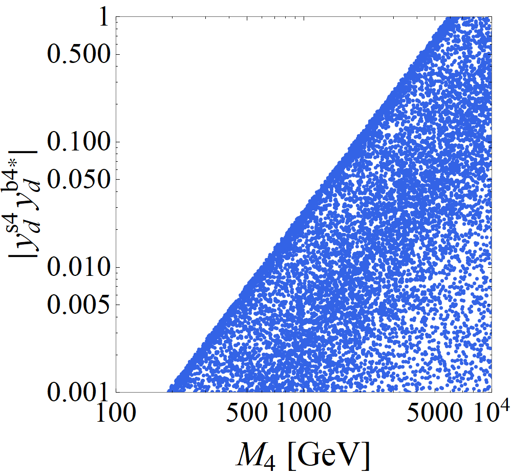
Using the definition of ZNCZ_{\mathrm{NC}} in Eq. (70), we obtain the constraint on the VLQ mass M4M_{4} and the product of the Yukawa coupling |yds​4ydb4∗||y_{d}^{s4}y_{d}^{b4*}|. This result is shown in the right figure of Fig. 10 where we use v=246v=246 GeV [36]. Since the constraint on rs​br_{sb} and θs​b\theta_{sb} from the Br[Bs→μ+μ−]Exp\mathrm{Br}[B_{s}\rightarrow\mu^{+}\mu^{-}]_{\mathrm{Exp}} is stronger than that from the Br[B¯→Xsγ]Exp\mathrm{Br}[\bar{B}\rightarrow X_{s}\gamma]_{\mathrm{Exp}} (See Fig. 10 left.), we show the region with blue dots where (M4,|yds​4ydb4∗|)(M_{4},|y_{d}^{s4}y_{d}^{b4*}|) satisfy the constraint from the Br[Bs→μ+μ−]Exp\mathrm{Br}[B_{s}\rightarrow\mu^{+}\mu^{-}]_{\mathrm{Exp}} and the quadrangle constraint Eq. (139). One finds that the lower limit on the VLQ mass is around 5.55.5 TeV for |yds​4ydb4∗|∼1\left|y_{d}^{s4}y_{d}^{b4*}\right|\sim 1.

Finally, we show the violation of the CKM unitarity on the complex plane in Fig. 11. The definition of each side is the same as that of Fig. 7. In order to obtain Fig. 11, we choose rs​b=0.018r_{sb}=0.018 and |θs​b|=π/6\left|\theta_{sb}\right|=\pi/6 and use the central values of the CKM matrix elements in Table 1. The side for λb​st\lambda_{bs}^{t} is connected with the real axis at (1,0)(1,0). The left figure is the case of θs​b=π/6\theta_{sb}=\pi/6 while the right figure is that of θs​b=−π/6\theta_{sb}=-\pi/6. One can see that the side for ZNCs​bZ_{\mathrm{NC}}^{sb} can be as large as that for λb​su\lambda_{bs}^{u} and the sign of θs​b\theta_{sb} affects the value of the angle βs\beta_{s} in Fig. 7.

Refer to caption
Figure 8: The dependence of Br[Bs→μ+μ−]VLQ\mathrm{Br}[B_{s}\rightarrow\mu^{+}\mu^{-}]_{\mathrm{VLQ}} on the FCNC coupling |ZNCs​b|\left|Z_{\mathrm{NC}}^{sb}\right|. The different colors of the dots represent the different ranges for the value of |θs​b||\theta_{sb}|. All the colored region satisfy the quadrangle constraint Eq. (139) with 0≤γs≤2​π0\leq\gamma_{s}\leq 2\pi. The experimentally allowed range of the branching ratio in Eq. (142) is shown as the blue shaded region. The horizontal solid line corresponds to the central value of the experimental branching ratio in Eq. (142).
Refer to caption
Refer to caption
Figure 9: The dependence of Br[B¯→Xsγ]VLQ\mathrm{Br}[\bar{B}\rightarrow X_{s}\gamma]_{\mathrm{VLQ}} on |ZNCs​b||Z_{\mathrm{NC}}^{sb}|. The different colors of the dots represent the different ranges for the value of |θs​b||\theta_{sb}|. All the colored region satisfy the quadrangle constraint Eq. (139) with 0≤γs≤2​π0\leq\gamma_{s}\leq 2\pi. The experimentally allowed range of the branching ratio in Eq. (144) is shown as the blue shaded region. The horizontal solid line corresponds to the central value of the experimental branching ratio in Eq. (144).
Refer to caption
Refer to caption
Figure 10: (Left) : The region allowed by the experimental data for the parameter rs​br_{sb} and θs​b\theta_{sb}. The blue dots satisfy both the constraint from the Br[Bs→μ+μ−]Exp\mathrm{Br}[B_{s}\rightarrow\mu^{+}\mu^{-}]_{\mathrm{Exp}} and the quadrangle constraint Eq. (139) with 0≤γs≤2​π0\leq\gamma_{s}\leq 2\pi. The green dots satisfy both the constraint from the Br[B¯→Xsγ]Exp\mathrm{Br}[\bar{B}\rightarrow X_{s}\gamma]_{\mathrm{Exp}} and the quadrangle constraint. (Right) : The constraint on the VLQ mass M4M_{4} and the product of the Yukawa coupling |yds​4ydb4∗||y_{d}^{s4}y_{d}^{b4*}|. The blue region satisfies the constraints from the Br[Bs→μ+μ−]Exp\mathrm{Br}[B_{s}\rightarrow\mu^{+}\mu^{-}]_{\mathrm{Exp}} and the quadrangle constraint Eq. (139).
Figure 11: The violation of the CKM unitarity on the complex plane. In order to obtain these figures, we choose (rs​b,θs​b)=(0.018,π/6)(r_{sb},\theta_{sb})=(0.018,\pi/6) in the left figure and (rs​b,θs​b)=(0.018,−π/6)(r_{sb},\theta_{sb})=(0.018,-\pi/6) in the right figure.

5 Summary and Discussion

We studied the model which includes one down-type SU(2) singlet VLQ in addition to the SM quarks and showed the constraints on the model parameters from Br[Bs→μ+μ−]\mathrm{Br}[B_{s}\rightarrow\mu^{+}\mu^{-}], Br[B¯→Xsγ]\mathrm{Br}[\bar{B}\rightarrow X_{s}\gamma] and the quadrangle relation. In order to analyze this model, we used the effective theory which is derived by integrating out the VLQ field. We assume that the mass of the VLQ is much larger than the EW scale. We matched the effective theory with the full theory not only at tree level but also at one-loop level and obtained the effective operators which are related to the radiative transition of the quarks. These operators correspond to the contribution from the diagrams including the VLQ in the internal line. One can find that the coefficient of the photon dipole operator with the down-type quarks is consistent with the case of the full theory calculation given in Ref. [17].

The other contributions to the radiative transitions come from the violation of the CKM unitarity and the diagrams which include the FCNC couplings among the SM quarks. We obtained the effective Lagrangian for the b→s​γ(∗)b\rightarrow s\gamma^{(*)} process arising from these contributions.

From our numerical results, we obtained the constraints on the FCNC coupling ZNCs​bZ_{\mathrm{NC}}^{sb} and the new physics parameters (rs​b,θs​b)(r_{sb},\theta_{sb}) defined in Eq. (111). We found that the dependence of Br[B¯→Xsγ]VLQ\mathrm{Br}[\bar{B}\rightarrow X_{s}\gamma]_{\mathrm{VLQ}} on θs​b\theta_{sb} is weaker than that of Br[Bs→μ+μ−]VLQ\mathrm{Br}[B_{s}\rightarrow\mu^{+}\mu^{-}]_{\mathrm{VLQ}} and the constraint on the model parameters rs​br_{sb} and θs​b\theta_{sb} from the Br[Bs→μ+μ−]\mathrm{Br}[B_{s}\rightarrow\mu^{+}\mu^{-}] is more stringent than that from the Br[B¯→Xsγ]\mathrm{Br}[\bar{B}\rightarrow X_{s}\gamma]. One can discriminate the cases of different |θs​b||\theta_{sb}| through the Br[Bs→μ+μ−]\mathrm{Br}[B_{s}\rightarrow\mu^{+}\mu^{-}] as shown in Fig. 8. When the |ZNCs​b||Z_{\mathrm{NC}}^{sb}| is order of 10−410^{-4}, the Br[Bs→μ+μ−]\mathrm{Br}[B_{s}\rightarrow\mu^{+}\mu^{-}] becomes small (large) for |θs​b|≃0​(|θs​b|≃π)|\theta_{sb}|\simeq 0~(|\theta_{sb}|\simeq\pi) compared with that of the SM. In Fig. 11, we showed the violation of the CKM unitarity on the complex plane when we chose rs​b=0.018r_{sb}=0.018 and |θs​b|=π/6|\theta_{sb}|=\pi/6. The difference in the sign of the θs​b\theta_{sb} affects the angle βs\beta_{s}, therefore we have to investigate the constraint from the observables related to the βs\beta_{s} to further restrict the form of the violation of the CKM unitarity.

Although we focused on the case of b→sb\rightarrow s transitions, the effective Lagrangian obtained in this paper can be applied to the FCNC transition for the other combinations of the down-type quarks. The 4-Fermi operators in Eqs. (23)-(25) and the effective Lagrangian for the off-shell photon contribute to b→s​l+​l−b\rightarrow sl^{+}l^{-} processes including B¯→K∗¯​l+​l−\bar{B}\rightarrow\bar{K^{*}}l^{+}l^{-}.

Finally, we add a comment on the renormalization group (RG) effect. One can not neglect the effect when the VLQ mass is much heavier than the EW scale. When M4/MW∼100M_{4}/M_{W}\sim 100, one may expect about 10% corrections to the Wilson coefficients. Moreover, the expressions of the FCNC coupling, CKM matrix elements and down-type quark masses will be modified. Including them, we will carry out the precise analysis elsewhere.

Acknowledgement

This work is supported by JSPS KAKENHI Grant Number JP16H03993 and JP17K05418 (T.M.). This work is also supported in part by Grants-in-Aid for Scientific Research [No. 16J05332 (Y.S.), Nos. 24540272, 26247038, 15H01037, 16H00871, and 16H02189 (H.U.)] from the Ministry of Education, Culture, Sports, Science and Technology in Japan.

References

  • [1] S. L. Glashow, J. Iliopoulos and L. Maiani, Phys. Rev. D 2 (1970) 1285.
  • [2] M. Kobayashi and T. Maskawa, Prog. Theor. Phys. 49 (1973) 652;  N. Cabibbo, Phys. Rev. Lett. 10 (1963) 531;  M. Gell-Mann and M. Levy, Nuovo Cim. 16 (1960) 705.
  • [3] J. Charles et al. [CKMfitter Group], Eur. Phys. J. C 41 (2005) no.1, 1 [hep-ph/0406184].
  • [4] M. Bona et al. [UTfit Collaboration], JHEP 0803 (2008) 049 [arXiv:0707.0636 [hep-ph]].
  • [5] Z. G. Berezhiani, Phys. Lett. 129B (1983) 99; Phys. Lett. 150B (1985) 177;   S. Rajpoot, Phys. Lett. B 191 (1987) 122; Phys. Rev. D 36 (1987) 1479;   A. Davidson and K. C. Wali, Phys. Rev. Lett. 59 (1987) 393;   Z. G. Berezhiani and R. Rattazzi, Phys. Lett. B 279 (1992) 124.
  • [6] K. S. Babu and R. N. Mohapatra, Phys. Rev. D 41 (1990) 1286.
  • [7] G. Barenboim, F. J. Botella and O. Vives, Nucl. Phys. B 613 (2001) 285 [hep-ph/0105306].
  • [8] F. J. Botella, G. C. Branco and M. Nebot, JHEP 1212 (2012) 040 [arXiv:1207.4440 [hep-ph]].
  • [9] A. K. Alok, S. Banerjee, D. Kumar and S. Uma Sankar, Nucl. Phys. B 906 (2016) 321 [arXiv:1402.1023 [hep-ph]].
  • [10] A. K. Alok, S. Banerjee, D. Kumar, S. U. Sankar and D. London, Phys. Rev. D 92 (2015) 013002 [arXiv:1504.00517 [hep-ph]].
  • [11] K. Ishiwata, Z. Ligeti and M. B. Wise, JHEP 1510 (2015) 027 [arXiv:1506.03484 [hep-ph]].
  • [12] C. Bobeth, A. J. Buras, A. Celis and M. Jung, JHEP 1704 (2017) 079 [arXiv:1609.04783 [hep-ph]].
  • [13] G. Aad et al. [ATLAS Collaboration], JHEP 1508 (2015) 105 [arXiv:1505.04306 [hep-ex]];  A. M. Sirunyan et al. [CMS Collaboration], arXiv:1708.02510 [hep-ex].
  • [14] F. del Aguila, M. Perez-Victoria and J. Santiago, Phys. Lett. B 492 (2000) 98 [hep-ph/0007160].
  • [15] F. del Aguila, M. Perez-Victoria and J. Santiago, JHEP 0009 (2000) 011 [hep-ph/0007316].
  • [16] C. Y. Chen, S. Dawson and E. Furlan, Phys. Rev. D 96 (2017) no.1, 015006 [arXiv:1703.06134 [hep-ph]].
  • [17] L. T. Handoko and T. Morozumi, Mod. Phys. Lett. A 10 (1995) 309,  Erratum: [Mod. Phys. Lett. A 10 (1995) 1733] [hep-ph/9409240].
  • [18] T. Inami and C. S. Lim, Prog. Theor. Phys. 65 (1981) 297,  Erratum: [Prog. Theor. Phys. 65 (1981) 1772].
  • [19] G. Buchalla, A. J. Buras and M. K. Harlander, Nucl. Phys. B 349 (1991) 1.
  • [20] G. C. Branco, T. Morozumi, P. A. Parada and M. N. Rebelo, Phys. Rev. D 48 (1993) 1167.
  • [21] G. C. Branco, P. A. Parada, T. Morozumi and M. N. Rebelo, Phys. Lett. B 306 (1993) 398.
  • [22] G. C. Branco, P. A. Parada, T. Morozumi and M. N. Rebelo, Nucl. Phys. Proc. Suppl. 37A (1994) no.1, 29.
  • [23] G. Barenboim and F. J. Botella, Phys. Lett. B 433 (1998) 385 [hep-ph/9708209].
  • [24] C. H. V. Chang, D. Chang and W. Y. Keung, hep-ph/9811354.
  • [25] K. I. Aoki, Z. Hioki, M. Konuma, R. Kawabe and T. Muta, Prog. Theor. Phys. Suppl. 73 (1982) 1.
  • [26] G. Buchalla, A. J. Buras and M. E. Lautenbacher, Rev. Mod. Phys. 68 (1996) 1125 [hep-ph/9512380].
  • [27] A. J. Buras, J. Girrbach, D. Guadagnoli and G. Isidori, Eur. Phys. J. C 72 (2012) 2172 [arXiv:1208.0934 [hep-ph]].
  • [28] B. Grinstein, R. P. Springer and M. B. Wise, Nucl. Phys. B 339 (1990) 269.
  • [29] M. Ciuchini, E. Franco, G. Martinelli, L. Reina and L. Silvestrini, Phys. Lett. B 316 (1993) 127 [hep-ph/9307364].
  • [30] A. J. Buras, M. Misiak, M. Munz and S. Pokorski, Nucl. Phys. B 424 (1994) 374 [hep-ph/9311345].
  • [31] A. J. Buras, hep-ph/9806471.
  • [32] K. G. Chetyrkin, M. Misiak and M. Munz, Phys. Lett. B 400 (1997) 206,  Erratum: [Phys. Lett. B 425 (1998) 414] [hep-ph/9612313].
  • [33] A. Ali and C. Greub, Phys. Lett. B 361 (1995) 146 [hep-ph/9506374].
  • [34] C. Greub, T. Hurth and D. Wyler, Phys. Rev. D 54 (1996) 3350 [hep-ph/9603404].
  • [35] N. Pott, Phys. Rev. D 54 (1996) 938 [hep-ph/9512252].
  • [36] C. Patrignani et al. [Particle Data Group], Chin. Phys. C 40 (2016) no.10, 100001.
  • [37] R. Aaij et al. [LHCb Collaboration], Phys. Rev. Lett. 118 (2017) no.19, 191801 [arXiv:1703.05747 [hep-ex]].
  • [38] Y. Amhis et al. [Heavy Flavor Averaging Group], arXiv:1612.07233 [hep-ex].
  • [39] B. Aubert et al. [BaBar Collaboration], Phys. Rev. D 77 (2008) 051103 [arXiv:0711.4889 [hep-ex]].
  • [40] J. P. Lees et al. [BaBar Collaboration], Phys. Rev. Lett. 109 (2012) 191801 [arXiv:1207.2690 [hep-ex]].
  • [41] J. P. Lees et al. [BaBar Collaboration], Phys. Rev. D 86 (2012) 052012 [arXiv:1207.2520 [hep-ex]].
  • [42] A. Limosani et al. [Belle Collaboration], Phys. Rev. Lett. 103 (2009) 241801 [arXiv:0907.1384 [hep-ex]].
  • [43] T. Saito et al. [Belle Collaboration], Phys. Rev. D 91 (2015) no.5, 052004 doi:10.1103/PhysRevD.91.052004 [arXiv:1411.7198 [hep-ex]].
  • [44] A. Abdesselam et al. [Belle Collaboration], arXiv:1608.02344 [hep-ex].
  • [45] S. Chen et al. [CLEO Collaboration], Phys. Rev. Lett. 87 (2001) 251807 [hep-ex/0108032].
  • [46] M. Misiak et al., Phys. Rev. Lett. 114 (2015) no.22, 221801 [arXiv:1503.01789 [hep-ph]].