YITP-18-04
KUNS-2714
RUP-18-2
Primordial Black Holes
- Perspectives in Gravitational Wave Astronomy -
Misao Sasakia, Teruaki Suyamab, Takahiro Tanakac,a, and Shuichiro Yokoyamad,e
a
Center for Gravitational Physics, Yukawa Institute for Theoretical Physics,
Kyoto University, Kyoto 606-8502, Japan
b
Research Center for the Early Universe (RESCEU), Graduate School
of Science,
The University of Tokyo, Tokyo 113-0033, Japan
c
Department of Physics, Kyoto University, Kyoto 606-8502, Japan
d
Department of Physics, Rikkyo University, Tokyo 171-8501, Japan
e Kavli IPMU (WPI), UTIAS, The University of Tokyo, Kashiwa, Chiba 277-8583, Japan
Abstract
This is a review article on the primordial black holes (PBHs), with particular focus on the massive ones () which have not evaporated by the present epoch by the Hawking radiation. By the detections of gravitational waves by LIGO, we have gained a completely novel tool to observationally search for PBHs complementary to the electromagnetic waves. Based on the perspective that gravitational-wave astronomy will make a significant progress in the next decades, a purpose of this article is to give a comprehensive review covering a wide range of topics on PBHs. After discussing PBH formation as well as several inflation models leading to PBH production, we summarize various existing and future observational constraints. We then present topics on formation of PBH binaries, gravitational waves from PBH binaries, various observational tests of PBHs by using gravitational waves.
1 Introduction
History of primordial black holes (PBHs) dates back to sixties when Zeldovich and Novikov pointed out that BHs in the early Universe may grow catastrophically by accreting the surrounding radiation [1]. In 1971, Hawking proposed [2] that highly overdense region of inhomogeneities in the primordial Universe can directly undergo gravitational collapse to form BHs, which initiated the modern mechanism of the PBH formation. Contrary to the astrophysical processes (i.e. collapse of stars) for which only BHs heavier than a particular mass (around 3 solar mass [3]) are possible to form, extremely strong gravitational force inside the highly compressed radiation/matter that can be realized in the early Universe allows formation of not only stellar/super-massive BHs but also small BHs that could be in principle as light as Planck mass (see e.g. [4] and references therein). After the advent of the inflationary cosmology, formation of PBHs and their properties such as mass and abundance had been studied in tight connection with inflation models. Conversely, knowledge of observational information about PBHs provides important clues to build inflation models. In particular, it is worth mentioning that even the non-detection of PBHs gives us useful information of the early Universe [4].
Observational searches of PBHs have been conducted intensively and continuously over several decades. Depending on the mass, PBHs trigger different observational signals. PBHs lighter than a certain mass given by [5]
| (1) |
have already evaporated by the cosmic age due to the Hawking radiation. Thus, PBHs lighter than do not exist in the present Universe. Nevertheless, they leave some traces from which we can investigate how many PBHs could have existed in the early Universe. For instance, PBHs in the mass range change abundance of light elements produced by the Big Bang nucleosynthesis due to high energy particles emitted by the evaporating PBHs [6]. Comparison between the observed light elements and the theoretical prediction tightly constrains the abundance of such PBHs (see e.g. [7] and references therein).
PBHs heavier than have not yet lost their mass significantly by the evaporation and remain in the present Universe. They not only imprint observational traces in the early Universe (such as by accretion, and indirect effects by the primordial density perturbations that seed PBHs) but also produce various distinct signals at present time such as gravitational lensing, dynamical effects on baryonic matter, and radiation emanating from the accreting matter into PBHs etc. What physical process among them becomes the most prominent to show us the existence of PBHs depends on the PBH mass. For instance, gravitational lensing of background stars is the most powerful method to search sub-solar PBHs (see Sec. 3). Accretion and dynamical effects on baryonic matter become more important for heavier PBHs. One of the important questions regarding non-evaporating PBHs is whether they comprise all the dark matter or not. Thanks to achievements of many different types of cosmological and astrophysical observations over decades, stringent upper limit on the PBH abundance has been obtained for a vast PBH mass range [8]. Currently, it appears that PBHs do not explain all the dark matter and at most constitute fraction of dark matter [9]. Reviewing the existing observational constraints on the non-evaporating PBHs is one of the main purpose of this article.
The LIGO discovery of the merger event (GW150914) of binary BHs [10] triggered a renewed interest of PBHs, especially in the stellar mass range. Unexpected largeness of the detected BHs (around ) brought us a new mystery about the component of the Universe. After the LIGO event, elucidating the origin of the BHs and binary formation has emerged as an important topic in cosmology and astrophysics (e.g. see [11]). Soon after the LIGO’s announcement on the first detection of the BH merger, several research groups [12, 13, 14] independently pointed out that the inferred merger rate can be explained by the merger of PBHs without violating the trivial bound that the PBH abundance is equal to or less than the total dark matter abundance. In [12, 13], binary formation by the accidental encounters of PBHs in dense environment, which works in the low-redshift Universe, has been considered, while different mechanism of the binary formation by the tidal perturbation caused by the distant PBHs, which works in the radiation dominated epoch in the early Universe and was originally proposed earlier in [15], has been investigated in [14]. These studies demonstrate that gravitational waves (GWs), brand new observable, provide a powerful and useful tool to probe parameter region of PBHs (mass, abundance etc) that have not been possible only by the electromagnetic waves. In other words, roles of GWs are complementary to electromagnetic waves.
In addition to the PBH scenario, several astrophysical processes such as the field binary scenario and the dynamical formation in the dense stellar environment have also been proposed to explain the observed properties of the binary black holes (for instance, see [11] and references therein). At the time of writing this article (autumn 2017), LIGO and Virgo detected five BH merger events [10, 16, 17, 18, 19]. For the moment, both the PBH scenario and the astrophysical scenarios are allowed as a possible explanation of these events because of a limited number of the detected events.
We are at the dawn of the golden age of the GW astronomy. In the future, the ongoing experiments such as LIGO and Virgo (and soon KAGRA) gain better sensitivity, and further upgraded and new type of experiments such as the Einstein Telescope [20], Cosmic Explorer [21], LISA [22], and DECIGO [23] covering different frequency bands will follow. Very likely, much more merger events will be detected and the statistical information of BHs and BH binaries such as mass, spin, eccentricity, redshift, spatial inhomogeneities, etc. will become available. Those information will enable us to test the individual scenarios and possibly to pin down the best one, or it is also conceivable that the truth is a mixture of multiple scenarios, e.g. some events due to PBHs and the others due to astrophysical BHs. In order to reveal the true nature of the BHs and their binaries, it is indispensable to go through three stages; to devise possible scenarios as many as we can (first), to theoretically understand each scenario and derive distinct features predicted in each scenario (second), and then to test the predictions by real observations and identify the answer (third). In addition to the main purpose as mentioned above, another purpose of this article is to review the PBH scenario in connection with the LIGO events and various proposals to test this scenario by using the future GW observations, i.e. the first and the second stages of the above classification.
Organization of this article is as follows. In the next section, we will review the basics of the PBH formation and related topics. Inflation models leading to the production of PBHs are also introduced. In Sec. 3, we cover various observational constraints on the abundance of non-evaporating PBHs obtained by the electromagnetic observations. Expected constraints in the future are also briefly presented. We do not put much focus on smaller PBHs that have already evaporated but briefly mention the constraints because they are less relevant to GWs. Regarding the constraints on such small PBHs, Ref. [7] provides a detailed analysis. In Sec. 4, we review the PBH scenario as an explanation of the LIGO events and future prospects of its observational test by GWs. Final section is a summary.
Throughout this article, we use a natural unit in which .
2 Formation of PBHs
Until now, several mechanisms to form PBHs in the early Universe have been proposed. As examples, Ref. [24, 25] recently discussed the possibility of PBH formation by domain walls and also Ref. [24, 26] proposed the PBH formation scenario by vacuum bubbles which nucleate during the inflation. There are also several works about the PBH formation from the cosmic string loops [27, 28, 29]. However, the most frequently studied PBH formation scenario must be a gravitational collapse of the overdense region in the early Universe. Here, we briefly review the formation process of the PBHs and also the inflationary models which could produce such an overdense region.
2.1 Basis of primordial black holes formation in the early Universe
2.1.1 PBH formation based on the simple physical picture
In the early radiation-dominated Universe, a highly overdense region would gravitationally collapse into a black hole, directly. Such a black hole formed in the early Universe is called primordial black hole (PBH). Details of the PBH formation from the overdense region in the early Universe has been extensively investigated numerically and analytically [30, 31, 32, 33, 34, 35, 36]. Here, let us give a brief review of a rough sketch of the PBH formation which unifies the traditional view based on the density contrast [37, 38] with the recent view based on the curvature perturbation [31, 39].
First, in the early Universe after inflation, the background spacetime can be well-described by the spatially-flat Friedmann-Lemaitre-Robertson-Walker (FLRW) metric (homogeneous and isotropic space):
| (2) |
where is a scale factor. From the Einstein equation, we can derive a background Friedmann equation as
| (3) |
where a dot denotes the derivative in terms of and is the background energy density.
On this background we consider a locally perturbed region that would eventually collapse to a black hole. Such a region will be a very rare region in the space. Hence, it may be approximated by a spherically symmetric region of positive curvature. Since the comoving size of such a region is initially much larger than the Hubble horizon size, one may apply the separate universe approach or the leading order spatial gradient expansion to it, that is, we may assume the metric of the form,
| (4) |
where and is assumed to be monotonically decreasing to zero as . It is known that the above form agrees with the metric on comoving slices on superhorizon scales, where corresponds to the nonlinear version of the conserved comoving curvature perturbation, that is [40]. The above metric can be cast into a more familiar form of a locally closed universe with the metric,
| (5) |
where the coordinates and are related to each other as , and is given by
| (6) |
We note that the 3-curvature of the const. hypersurface is given by
| (7) |
Ignoring the spatial derivative of in the spirit of leading order gradient expansion, the time-time component of the Einstein equations (the Hamiltonian constraint) gives
| (8) |
where . This is equivalent to the Friedmann equation except for a small inhomogeneity induced by the curvature term. One could regard this as the Hamiltonian constraint on the comoving hypersurface, or that on the uniform Hubble hypersurface on which the expansion rate is spatially homogeneous and isotropic.
The above equation naturally leads us to define the density contrast on the comoving hypersurface by
| (9) |
From the fact that during the radiation-dominated universe, this is vanishingly small initially, being consistent with the picture that it is the curvature perturbation that induces the density perturbation.
As the universe evolves grows to become of order unity. If we would ignore the spatial dependence of , the universe with would eventually stop expanding and recollapse. This happens when , namely when the comoving scale of this positively curved region becomes of the order of the Hubble horizon scale, at which our separate universe approximation precisely breaks down. Also the equivalence between the comoving and uniform Hubble slices no longer holds. Nevertheless, we may expect that Eq. (8) will still be used in obtaining a qualitatively acceptable criterion for the black hole formation, which has been actually shown to be valid in fully nonlinear numerical studies.
Since is the time when the universe stops expanding if it were homogeneous and isotropic, let us assume this epoch to be the time of black hole formation, . Since a perturbation on scales smaller than the Jeans length cannot collapse, we set this to happen at or for . Namely, we have
| (10) |
This implies we should identify with . It is then straightforward to find the criterion for the black hole formation. The condition is that the comoving slice density contrast at the time when the scale of interest re-enters the Hubble horizon is greater than ,
| (11) |
where is the time at which #1#1 #1 Originally, in Ref. [37] there was an upper bound on in order to avoid the formation of the separate closed universe. However, recently Ref. [41] pointed out that this is not the case. Actually from the point of view of the curvature perturbation on comoving slices, it is by definition the fact that can never exceeds unity on superhorizon scales. .
Within the scope of the present level of approximation, it is not meaningful to distinguish between the Jeans length, , and the Hubble horizon. Crudely speaking, the mass of the formed PBH is equal to the horizon mass at the time of formation.
In the above, we have presented a basis of the PBH formation out of the primordial perturbation based on the simple physical picture. Although such analysis captures the essence of the PBH formation, it is also important to clarify the impact of the various effects that have been ignored in the above discussion, which are addressed below.
2.1.2 Precise value of the threshold
The equation (11) only tells us that the PBH formation occurs when the density perturbation becomes comparable to . A precise value of the threshold for PBH formation has been extensively investigated both numerically and analytically [30, 31, 32, 33, 34, 35, 36]. For instance, Ref. [36] has derived a new analytic formula for the threshold as for the uniform overdense profile surrounded by the underdense layer, where is the amplitude of the density perturbation at the horizon crossing time in the uniform Hubble slice and is the equation of state of the dominant component in the Universe at the formation. Although the analytic formula given above shows good agreement with the results of the numerical simulations, numerical simulations also demonstrate that there is no unique value of the threshold. Different density/curvature perturbation profiles collape to BH above the different threshold, which is quite natural from the physical point of view. In terms of the comoving density perturbation, the spread of the threshold was found to be . Interestingly, the value , which have been obtained in the crude approximation, lies in this range. Notice that the spread changes if we use perturbation variable defined in the different time slicing.
2.1.3 Effects of long wavelength modes
The physical picture presented above shows that PBHs can form when the size of the overdense region becomes equal to the Hubble horizon. Because of causality, any additional large-scale perturbations longer than the Hubble horizon at the time of the PBH formation must not affect the PBH formation. However, this is not explicitly visible for some perturbation variables.
For example, if we use the curvature variable on the uniform Hubble slicing, which is identical to the comoving curvature perturbation on super-horizon scales (and is also equal to the curvature perturbation on uniform energy density slicing ), the threshold depends on how much the longer wavelength modes are. The reason for this is that the curvature variable is not the local quantity but the quantity which requires information of the distant distribution of matter for it to be determined [42]. Although one can in principle use the curvature variable (or any other perturbation variables as long as it is well-defined) for computing any observables such as the abundance of the PBHs, appropriate prescription is needed to obtain the correct results if the considered perturbation variable is not local.
In Ref. [39], the formation criterion is discussed in terms of the spatial 3-curvature and the density contrast both of which naturally suppress the super-Hubble modes. Actually the picture we presented in the above is based on this approach. As clear from Eq. (7), it is the spatial derivative of that determines the 3-curvature, and when normalized with the background expansion term , it approximately equal to the density contrast on the comoving hypersurface , as defined in Eq. (9). Use of these quantities would be especially convenient when one studies the PBH formation out of the inhomogeneities which are randomly distributed and whose overdensity regions are non-spherical.
2.1.4 Near critical collapse
It is known that when the overdensity is very close to the threshold there is a simple scaling-law for the mass of the formed black holes as [43, 44, 45]
| (12) |
In Refs. [30, 46], based on the above scaling-law, the mass function of the PBHs has been calculated. The results show that the typical mass of the PBHs is still about the horizon mass evaluated at the time of formation. Yet, since the critical collapse produces smaller mass PBHs, mass function has a power-law tail for the smaller mass range. This could be important when one tries to precisely adopt the observational constraint for the abundance of PBHs with extended mass spectrum to constrain inflation models [8, 47].
2.1.5 Non-sphericity of the overdense region
In the above discussion, the criterion for the PBH formation is considered for an isolated spherically symmetric perturbation where the universe approaches a perfectly homogeneous and isotropic spatially flat universe in the large scale limit. In reality, any overdense region for the random density perturbation is generically not completely spherically symmetric. Yet, compared to the studies of the PBH formation out of the spherically symmetric over density, studies on how the non-sphericity affects the PBH formation are short. In Ref. [48], non-spherical overdense region was approximated as ellipsoid, and it was demanded that spherical region enclosed by the shortest axis of the ellipsoid satisfies the collapse criterion for the spherical overdensity as the collapse condition. Then, combining the above condition with the Carr’s argument [37] that relates the density contrast at the time of horizon crossing to the mass of the overdense region, it was shown that the threshold density contrast of the ellipsoid over density is given by
| (13) |
where is the ellipticity of the ellipsoid and is the threshold for the spherical overdensity. This shows that larger density contrast than the spherical one is needed for the non-spherical overdense region to turn into the PBH. Although the numerical value on the right hand side of Eq. (13) is obtained by the crude approximation in [48], this result is qualitatively natural since more overdensity is needed than the spherical case to pull the overdense region along the longest axis by gravity. Thus, for primordial density perturbations obeying the probability distribution function for which higher-sigma peaks are more suppressed, which are realized in most inflation models, the overdense regions for the PBH formation are nearly spherically symmetric. More quantitative argument is possible if we further assume the Gaussianity for the density perturbations. In this case, typical value of the ellipticity for the peak amplitue much greater than the square root of the variance () is given by
| (14) |
Thus, if the PBHs are formed out of the -sigma peaks, the degree of the non-sphericity for the overdense regions is suppressed by [49, 50, 48].
2.1.6 PBH formation during a matter-dominated-like era
Finally let us mention the case of PBH formation during a matter-dominated era. Of course, primordial black holes may also form in the matter-dominated era, and it has been also discussed in the literature, and it has been emphasized that taking account of deviations from spherical configurations is essential [51, 52, 53]. Besides, in reality the matter cannot be exactly dust with but it behaves either as a fluid with small pressure or as a collisionless fluid. These effects should be very important but they have not been fully explored yet. The massive scalar field is known to behave like a non-relativistic matter when it oscillates around the potential minimum. Thus, for models of inflation in which the inflaton or another scalar field oscillates after inflation and dominates the universe, the PBH formation during that era may become important [54, 55, 56].
2.2 Clustering of PBHs
Let us consider a simplified situation where primordial perturbations consist of two components, short and long wavelength modes, and PBHs are formed out of the short wavelength modes (see Fig. 1). We denote by and the representative comoving wavenumbers of the short and long wavelength modes, respectively (). At the time of the horizon crossing , the long wavelength modes are still super-Hubble and such modes are absorbed into the homogeneous component on the Hubble scale .
If there are no correlations between the short and long wavelength modes, which is the case for the perturbations obeying the Gaussian statistics, spatial distribution of PBHs at the formation time should not trace the large scale perturbations. In fact, adopting the comoving density contrast as the perturbation variable and the peak-background picture, it was shown [57] that the effect of the large scale perturbations is significantly suppressed. In other words, PBHs are little clustered initially on the comoving scale #2#2 #2 It has been claimed in Ref. [58] and later in Refs. [59, 13] that PBHs are clustered initially even for the Gaussian density perturbations. As far as the authors are concerned, there is not a broad consensus on this possibility. . Their spatial distribution is uniform and the number density fluctuates according to the Poisson statistics. Notice that even if the PBHs are not clustered initially, they can later cluster by the gravitational potential created by the long modes just like the formation of dark matter halos in the CDM scenario.
If, on the other hand, the short modes correlate with the long modes, it can happen that the amplitudes of the short modes modulate by the long modes. One example is the local-type non-Gaussianity for which the curvature variable on super-Hubble scales can be written as
| (15) |
where is a Gaussian variable containing both short and long modes and is the so-called non-linearity parameter [60] which is dimensionless and constant #3#3 #3 The definition of in Eq. (15) is different from the standard one by a factor . We have omitted this unessential factor to make equations simple. . This type of perturbation arises when the initially isocurvature modes are converted to the adiabatic modes. Decomposing into the short mode and the long mode as
| (16) |
we find that can be written as
| (17) |
where and are defined by
| (18) |
By definition, hold. Then, ignoring the terms suppressed by a factor , the 3-curvature given by Eq. (7) can be written as
| (19) |
where is the local scale factor. For , given above represents space curvature on the comoving scale . Since contains the long mode , the magnitude of the short mode 3-curvature modulates over the comoving scale . As a result, PBH number density also modulates on the comoving scale , and PBHs are clustered on the large scale . For more details, see Refs. [61, 57].
2.3 Abundance of PBHs
In order to investigate the abundance of formed PBHs, let us introduce a parameter which represents the mass fraction (the energy density fraction) of PBHs at the formation as , which can be defined as
| (20) |
where is a Hubble parameter, and are respectively a fraction of PBHs against the total dark matter component and a density parameter of the matter component at present, and “form” and “”, respectively, denote the values evaluated at the formation and the present time. As we have mentioned in the previous subsection, the mass of PBHs formed in the radiation dominated era can approximately be evaluated to be equal to the horizon mass, with being the total energy density of the Universe), at the formation, and hence we have
| (21) | |||||
| (23) |
Here, we introduce a correction factor, , which can be evaluated as in a simple analytic calculation [37]. By using the above relation between the mass of PBHs and the Hubble parameter at the formation, mass fraction of PBHs, , can be written as (e.g., [7])
| (24) |
where is a number of relativistic degree of freedom. Thus, for each mass of PBHs, the observational constraint on can be interpreted as that on .
As we have shown in the previous subsection, during radiation-dominated era, PBHs are basically considered to be formed when a sufficient overdense region, corresponding to the density fluctuations with a sufficiently large amplitude at a certain scale, enters the Hubble horizon. Once the probability distribution function of the density fluctuations is given, can be regarded as the probability that the density contrast is larger than the threshold for PBH formation, and we can evaluate the mass fraction as
| (25) |
where is the threshold for PBH formation. For the Gaussian distribution function, is approximately given by
| (26) | |||||
| (28) |
where is the variance of the density fluctuations on the mass scale , and #4#4 #4 Ref. [53] found that for the PBH formation in the matter dominated era the production probability of PBHs, , is approximately given by for . Here, is a variance of the density fluctuations at the horizon re-entry.. The variance is estimated as
| (29) |
where and are, respectively, the power spectra of the primordial density fluctuations and the curvature perturbations on comoving slicing and is a window function smoothing over the comoving scale . Here, we assume . Then, from the above expression, we can interpret the constraint on as that on which corresponds to the amplitude of the density fluctuations. Furthermore, it would give a hint for constructing the successful inflationary models with PBH formation. As an example, if the constraint on for would be obtained as , which is equivalent to , it could be interpreted as , that is, with .
For the primordial power spectrum with a broad peak, it should be useful to give an expression for the mass function, which represents the fraction of PBHs with mass in . It can be defined as
| (30) |
with
| (31) |
and
| (32) |
Here, , and we have assumed the Gaussian distribution function for the primordial density fluctuations and .
There are several works about the effect of the non-Gaussianity in the estimation of [62, 63, 64, 65, 66, 67, 68, 69]. In principle, the non-Gaussian feature of the statistics of the primordial curvature perturbations would strongly depend on the generation mechanism of the primordial fluctuations, that is, the inflation models, and we should evaluate for each exact form of the probability distribution function . However, it might be hard task to evaluate the exact form of the probability distribution function for each inflationary model, and hence it should be convenient to give an approximate formulation to take into account the non-Gaussian effect. One of such formulations can be considered by the cumulant expansion of the probability distribution functions [65]. In the standard single slow-roll inflation, the higher order cumulants are expected to be suppressed by the slow-roll parameter. However, as shown in the next subsection, for efficient PBH formation we need to consider non-standard inflationary models with the violation of the slow-roll condition. Thus, the effect of the non-Gaussianity can be relevant for some inflationary models [67].
2.4 Generating seeds of PBH from inflation
Here, we focus on the mechanism where the PBH formation is induced by the primordial density fluctuations, and we give a review of inflationary mechanism which could generate seeds of the PBHs, that is, primordial curvature perturbations with large amplitudes at a certain scale.
For preparation, let us give a relation between the mass of PBHs and the comoving wavenumber of the perturbations. Basically, as we have discussed in the previous subsection, PBH could be formed when an overdense region enters the Hubble horizon. If such an overdense region is sourced from the primordial curvature perturbations, the size of the overdense region should be characterized by the comoving wavenumber of the primordial perturbations, . Then, we can obtain the relation between the Hubble scale at the PBH formation and the comoving wavenumber of the sourced primordial curvature perturbations as
| (33) |
During the radiation dominated era, we have and hence the relation between the comoving wavenumber, , and the Hubble parameter at the formation as . Substituting the relation between and into the above expression for , we can obtain the relation between the mass of PBHs and the comoving wavenumber as [70]
| (34) |
From this equation, we find that a hierarchy between the observable scales by CMB observations and -PBHs is given by#5#5 #5 Here, we use a pivot scale in Planck 2015 as a typical observable scale by CMB observations, .
| (35) |
On the other hand, the number of -folds measured from the time when the present horizon scale exits the Hubble horizon during inflation to the end of inflation is required to be typically -. Thus, based on the above discussion, we find that, if we want to form PBHs from the primordial density perturbations, we need to consider some mechanism which can amplify the perturbations during the inflationary phase#6#6 #6 Refs. [71, 72, 73, 74, 75] discussed the PBH formation during QCD phase transition era with the assumption that the phase transition is first order. However, currently the QCD phase transition has been known to be not first order but a crossover, and hence the efficient PBH formation during QCD epoch might be difficult..
2.4.1 Single-field inflation
First, let us consider the possibility of generating PBHs in the standard slow-roll inflationary scenario. For the single-field standard slow-roll inflation, the power spectrum of the primordial curvature perturbations on comoving slicing is given by
| (36) |
where is the time derivative of the inflaton field and the subscript “” represents the value at a time when the scale of interest exits the Hubble horizon during inflation. For the power-law ansatz;
| (37) |
Eq. (36) gives a power-law index as#7#7 #7 This expression is derived based on the slow-roll equations:
| (38) |
where and are slow-roll parameters which can be characterized in terms of the potential of the inflaton field as
| (39) |
where and . Thus, positive large can realize the blue-tilted power spectrum, that is, larger amplitude for smaller scales (larger comoving wavenumber).
Current CMB observations have indicated that is about (often called as COBE normalization) over CMB observable scales and the PBH formation is effective enough to be observationally-interesting for . Thus, if we want to realize such a large amplitude at by blue-tilted power spectrum, consistent with the COBE normalization, we need
| (40) |
For successful inflation, we need to require . Hence, the above value for the spectral index seems to be large and it is not so easy to realize in the standard inflationary models. Furthermore, we have a strong constraint on the spectral index obtained from CMB observations, e.g., from the Planck observation, we have [76]
| (41) |
Thus, for the PBH formation, even if we can realize the blue-tilted power spectrum, the single power-law model should be in conflict with the CMB observations.
Running mass inflation model
One possibility of realizing relatively large blue-tilted inflationary model consistent with the Planck result is large running mass inflation model [77, 78, 79]#8#8 #8 Here, we focus on inflation models which could produce PBHs with . Smaller PBHs formation in a running mass inflation model has been discussed also in [80, 81, 82, 83].. In this model, the time dependence of during inflation could be large, that is, the scale-dependence of could also become large (see, e.g., [84, 85])#9#9 #9 Note that, in order to realize the end of inflation, this type of model needs a hybrid-inflation-type mechanism with a waterfall field other than the inflaton. In this sense, the running mass inflation model is not strictly a single field model [85].. Thus, when remains to be small so as to be consistent with the Planck result on CMB scales, but takes a positive larger value on smaller scales, we can realize the large amplitude of primordial curvature perturbations on an appropriate small scale which could be seeds of PBHs. For such kind of models, the primordial power spectrum is not a simple power-law (37), but the one that includes the scale-dependence of the spectral index perturbatively:
| (42) |
where and are, respectively, called “running of spectral index” and “running of running” parameters. In the standard slow-roll inflation models, and are highly suppressed by slow-roll parameters. However, in the large running mass inflation model, these parameters would be relatively large. For the above parameterization, in order to produce PBHs with on CMB scales, we need to take to be about 0.1 as shown by the red line in Fig. 3.
However, assuming the negligibly small running of running parameter , for such a large PBHs with smaller masses (corresponding to larger comoving wavenumbers) would be overproduced. To avoid the overproduction of smaller PBHs, we need to have a cutoff in the primordial power spectrum at an appropriate scale. Based on the parameterization given as (42), such a cutoff can be realized by taking into account non-negligible running of running . As shown in Fig. 3, by employing appropriately tuned positive and negative , one can realize a broader peak in the power spectrum and it predicts the broad mass spectrum of PBHs.
Recent Planck result gives constraints not only on the spectral index , but also on the running of the spectral index as [86]
| (43) |
Thus, by comparing this observational constraints with the value for shown in Fig. 3, we find that it is difficult to construct a viable inflationary model which can produce PBHs based on the perturbative scale-dependent spectral index (42).
Inflection inflation model

Ref. [87] recently proposed a single field model which can produce the primordial power spectrum with a peak. They consider the inflaton’s potential with a inflection (plateau) point where the inflaton temporarily slows down during inflationary phase. PBH formation in such an inflationary scenario with a “plateau” in the scalar potential was discussed in Ref. [88]. Ref. [88] calculated the spectrum of the adiabatic perturbations for the schematic representation of the scalar potential which has two breaks and a flat plateau between these breaks#10#10 #10 Ref. [62] also studied PBH formation in several toy models.. The reason why such a model can produce a peak in the primordial spectrum can be easily understood as follows. Let us recall the expression of the primordial power spectrum given by (36). This expression can be rewritten in terms of the slow-roll parameter as
| (44) |
From this expression, one can find that when the inflaton temporarily slows down, the slow-roll parameter becomes more suppressed and the power spectrum have a peak at the scales which exit the Hubble horizon during the slow-down phase. However, if the plateau is completely flat there appears a problem that the inflaton may stay too long at the plateau and the inflationary phase eternally continues, so-called eternal inflation. To avoid this problem, in Ref. [87], a “near”-inflection point has been introduced in the inflaton potential. Such kind of models in the context of PBH formation have also been discussed in Refs. [89, 90, 91, 92].
In fact, as pointed out in Ref. [92], the standard slow-roll conditions might be generally violated near the inflection point. In the standard slow-roll approximation, we approximate where and is an inflaton field, and this means that in the equation of motion of the inflaton we can neglect the acceleration of the inflaton, , term. However, if becomes too small as around the inflection point, in the equation of motion term would become balanced with term, that is, . Thus, the above discussion based on the slow-roll parameters would be violated. In fact, based on the detailed calculation, in such an inflection-point inflation, the amplification of the primordial density fluctuations can be realized, but at most [87, 92].
This type of model tends to predict broader peak, , in the primordial power spectrum, and hence the mass spectrum of the formed PBHs would also be broader [87].
Single-field chaotic new inflation model
Ref. [64, 65] proposed the possibility of PBH formation in the context of double inflation even for the single field case, called chaotic new inflation. In this scenario, the inflaton potential is basically given by so-called Coleman-Weinberg or double-well type potential which have been studied in the context of new inflation scenario (Fig. 5).
In the standard new inflation scenario inflation is caused by an inflaton which starts slow-roll from the vicinity of the origin which is an unstable local maximum. On the other hand, if the initial amplitude of the scalar field is Planck scale largely exceeding the global minimum, it causes chaotic inflation. For such kind of potential, if we tune the model parameters, two inflationary phases could be realized. As a first phase of inflation, chaotic inflation occurs with a large field value of the inflaton. After the phase of chaotic inflation, the inflaton oscillates around the origin as well as in the standard chaotic inflationary model. However, in this model the potential has a feature which can realize new inflation around the origin. Thus, after the oscillation, with some tuning of the model parameters, new inflation occurs as a second phase of the inflation.
In this scenario, the amplification of the primordial curvature perturbations would be expected to be efficient for the modes which exit the horizon at the transition era from the first phase to the second, where the slow-roll conditions are temporarily violated. As in the case of the inflection point inflation model, around the local maximum the slow-roll conditions are temporarily violated and then the enhancement of the curvature perturbations occurs. This model would predict relatively-sharp peak in the power spectrum of the curvature perturbations, , and PBH mass spectrum becomes even narrower[65].
2.4.2 Multi-scalar inflation
Next, let us consider multi-scalar inflation models which can produce seeds of PBHs, i.e., the primordial curvature perturbations with large amplitudes.
double inflation model

As we have discussed in single-field inflation case, if we have a phase where the inflaton temporarily slows down during inflation, corresponding to the very flat region in inflationary potential, we can realize a peak in the primordial power spectrum at an appropriate scale. The important point in the above models to realize the enhancement of the primordial curvature perturbations to form PBHs during inflationary era is temporal violation of the standard slow-roll conditions. In case of multi-scalar models, such kind of feature in the inflation dynamics could be easily realized [93, 94]. Ref. [95] investigated the possibility of PBH production in the context of hybrid inflation, where inflationary dynamics depends on two scalar fields.
In the original types of hybrid inflation, one scalar field which possesses a false vacuum energy is assumed to be massive, and inflation was driven by this false vacuum energy. Another field slow-rolls down the flat potential, and when it reaches a critical value, the massive field becomes tachyonic and inflation abruptly ends. In general, we can also consider the case where both fields existing in hybrid inflation are not massive #11#11 #11 Non-Gaussianity of the super-Hubble perturbations in this case was shown to be very tiny [96].. In such a case, we can realize two stages of inflation (double inflation) and a phase of the transition. Basically, in the phase of the transition, fields roll down the very flat region in the potential and hence the primordial curvature perturbations which exit the Hubble horizon during this phase may be amplified, as we have discussed in the inflection model.
Now lots of models in the context of double inflation have been proposed for PBH formation[59]. Refs. [70, 97, 98] discussed the construction of such double inflation models in supergravity, named smooth hybrid new inflation.
In this type of scenarios, the expected power spectrum of the curvature perturbations strongly depends on the details of the models. As an example, as shown in Refs. [70, 99, 100], the expected power spectrum has two peaks, one of which is very sharp and the other is much broader.
curvaton model
Another possibility of generating the primordial curvature perturbations with large amplitude at a certain scale can be considered in the context of so-called curvaton scenario. In the simple curvaton scenario, we have two scalar fields, one (called inflaton) is responsible for the accelerating expansion of the Universe, that is, inflation, and the other (called curvaton) responsible for generating the primordial curvature perturbations. As we have mentioned, one of the difficulties of PBH formation in the single field inflation is that we should realize the large amplitude of fluctuations at a small scale for PBH formation and the COBE normalization on the CMB scales for the primordial curvature perturbations, simultaneously. In some extension of the simple curvaton scenario, the primordial curvature perturbations could be generated both from the inflaton and the curvaton fluctuations. Thus, if we can construct a model in which the primordial curvature perturbations on the CMB scales are generated from the inflaton fluctuations while those on small scales are generated from the curvaton fluctuations, we can realize a successful inflationary model for PBH formation consistent with the CMB observations [38, 101, 102]#12#12 #12 In Ref. [103], PBH formation has been discussed in the scenario where the curvaton induces a second inflationary phase..
Basically, in this curvaton scenario, the power spectrum of the curvaton fluctuations (primordial isocurvature perturbations) has a cut-off on a large scale and a scale-invariant feature on smaller scales. During the radiation dominated era after the reheating, the curvaton field starts to oscillate and it behaves as a non-relativistic matter. Thus, the energy density of the curvaton field gradually gets to contribute to the total energy density of the Universe and it means that the curvaton fluctuations, which are initially isocurvature perturbations, are gradually transformed into the adiabatic curvature perturbations, i.e., the adiabatic curvature perturbations grow in time. In the standard curvaton scenario, the curvaton decays into the radiation at a certain time. After the curvaton decays, the adiabatic curvature perturbations become constant in time. As shown in Fig. 7, in this scenario the both components of primordial curvature perturbation spectra at the horizon re-entering are smooth. Thus, the mass spectrum of the formed PBHs would be broad. In [104], it was shown that if there are multiple curvaton fields, they can temporarily enhance the curvature perturbations on all super-Hubble scales and the PBHs could be copiously produced during those modes re-enter the Hubble horizon until the enhancement terminates #13#13 #13 The temporal enhancement of the curvature perturbations and the PBH formation were also studied in the case where the non-inflaton field has a Galileon-type kinetic interaction [105]. . There are also several models where the primordial curvature perturbations were enhanced by non-trivial interactions between the inflaton and some fields, e.g., a gauge field [106].
3 Observational constraints on non-evaporating PBHs
In this section, we review how the upper limit on the fraction of PBHs in dark matter can be obtained for various mass range of non-evaporating PBHs (). Broadly speaking, constraints are divided into direct and indirect ones. The direct constraints are derived by investigating the observational effects that PBHs directly trigger by their gravitational potential and are thus independent of the mechanisms of the PBH formation. The direct constraints can be further classified into four categories by the manners PBHs affect: gravitational lensing, dynamical effect, the accretion, and the growth of large scale structure. All these topics are covered in this section. Indirect constraints are those that can be obtained by the observational effects that are not caused by the PBHs but something else which is deeply connected to PBHs. Although such constraints cannot be applied to all the possible PBH scenarios, they are powerful in excluding some of them. Several known indirect constraints are also reviewed in the latter part of this section.
The existing constraints will be tightened (or may be replaced by the detection of PBHs) in the future both by the improvement of the apparatuses similar to the existing ones and the launch of the qualitatively new observations such as lines. Future constraints are also briefly touched at the end of this section.
All the constraints discussed in this section are based on the electromagnetic signals. The new observable, namely gravitational waves, in the context of PBHs is the topic in the next section. It is important to keep in mind that all the constraints in this section are derived under the assumption that the PBH mass function is monochromatic, which is valid when the width of the mass function is sufficiently narrow. The case for a broad mass spectrum requires separate analysis, which will be briefly addressed at the last part of this section.
Before ending the introduction of this section, we briefly mention the constraints on the PBHs lighter than that have already evaporated or are in the final state of evaporation by the Hawking radiation [7]. Although those PBHs, depending on their mass, do not exist or are fading at the present epoch, high-energy partciles emitted from PBHs leave some signals from which we can place the upper limit on the PBH abundance. They include production of the lightest supersymmetric particles (if they exist) (, entropy production in the early universe (, change of the abundance of the light elements produced by the big bang nucleosynthesis (, extragalactic photon background (, and damping of the CMB temperature anisotropies on small scales by modifying the cosmic ionization history (. By comparing these effects with observations, upper limits on the PBH fraction defined by Eq. (20) for various PBH mass (assuming monochromatic mass function) can be obtained (for comprehensive study on this topic, see Refs. [7, 107]). Except for the constraints from the entropy production and the primordial helium abundance, these limits are severe in the sense that they allow only a tiny fraction of PBHs in dark matter at any cosmic time before the PBHs evaporate. Assuming Gaussianity of the primordial perturbation, these limits can be converted to the upper limit on the power spectrum of the curvature perturbation as for [107]. Although the upper limit on varies many orders of magnitude over the PBH mass range corresponding to the above range of , the upper limit in terms of is insensitive to , which is traced back to the fact that depends on the exponentially. (see Sec. 2.3).
3.1 Gravitational lensing
Gravitational lensing is a very powerful method to constrain/detect PBHs. Excellent point of the gravitational lensing is that the individual lensing signal is solely based on the gravitational physics and does not suffer from the uncertainties that exist in the studies of electromagnetic signals resulting from the interaction between the PBHs and the surrounding matter.
If PBHs are present in the Universe, they cause the gravitational lensing on the background objects such as stars. Under the thin-lens approximation in which the deflection of light occurs at a point on the lens plane (which is a very good approximation in the astrophysical situations we are considering), the lens equation can be written as (Fig. 8)
| (45) |
In terms of the distance on the lens plane , the lens equation becomes
| (46) |
where and is the Einstein radius. Thus, the positions of the lensed images are given by
| (47) |
There are thus two lensed images at and . The only exception is when the source, lens object, and the observer are on the same line, i.e. . In this case, the image on the lens plane becomes a circle (the so-called Einstein Ring) with its radius given by . Lensing effect becomes significant when and typical angular separation of the two images is
| (48) |
where we have introduced the parametrization as .

3.1.1 Microlensing
Gravitational microlensing refers to the gravitational lensing event in which the angular separation of the images lensed by a compact object is so small that the individual images cannot be resolved by observations [108]. For instance, the angular separation given by Eq. (48) is much smaller than the angular resolution of the existing (or past) microlensing experiments such as the MACHO Project and EROS collaboration which is about . In the gravitational microlensing event, what can be observed is only the superposition of two images which is brighter than the original source. The magnification factor , normalized to unity in the absence of the microlensing, is given by
| (49) |
At , . When the lens object is moving relative to the line of sight connecting the source and the observer, becomes time-dependent and the magnification varies in time. Assuming a constant tangential velocity , we can write as
| (50) |
where is the impact parameter of the source in the lens plane and the origin of is chosen so that the source image in the lens plane becomes the closest to the lens object at . Magnification curves for various values of are given in Fig. 9. As we can see, the magnification is maximum at and symmetric about it. The time scale for the rise and fall-off of the magnification is given by
| (51) |
We find that the time scale is longer for larger lens mass and larger distance to the source.
A useful quantity which is used in the context of the microlensing is the optical depth [109, 110]. This quantity measures how likely a background source is micro-lensed by the compact objects with magnification factor greater than #14#14 #14 The actual threshold for for the detection of the microlensing event depends on the detection methods in individual experiments. The value is just for convenience.. In other words, the optical depth, when it is much smaller than unity, is the probability that the light from the source passes inside the circle defined by the Einstein radius on the lens plane. Assuming that all the lens objects have the same mass, the optical depth can be written as
| (52) |
where is the energy density of PBHs. Interestingly, the last expression of the optical depth shows that it does not depend explicitly on the mass of PBHs. What determines the optical depth is how much PBHs constitute the entire dark matter.
In 1986, Paczyński pointed out that it would be possible to test the hypothesis that some fraction of dark matter is in the form of compact object by monitoring a few million stars in the Magellanic Clouds [111]. Light from any star in MC passes through the dark matter halo encompassing the Milky Way Galaxy before it reaches the observer on the Earth. If the dark matter halo entirely (or partially) consists of the compact objects, they produce microlensing events on the source stars in MC. According to the estimate in [111], the optical depth for the microlensing event is given by
| (53) |
If , about one star among a few million stars must produce a microlensing event. Conversely, non-observation of microlensing events places the upper limit on the PBH abundance. The time scale of the magnification is for and minutes for (see Eq. (51)). Thus, the few year observation of the stars in MC enables us to place constraint on the PBHs with up to .
It is important to mention that there is a lower limit on the PBH mass below which the finite-size effect of the source changes the magnification by the microlensing from that in the point lens case. The finite-size effect becomes relevant when the angular size of the source star projected on the lens plane becomes comparable to or larger than the angular size of the impact parameter . The peak magnification becomes smaller or larger than that in the case in the point lens depending on the magnitude relation between the projected source size and [112]. Especially, when is much smaller than the source size, the maximum of becomes
| (54) |
Thus, becomes close to unity for . In terms of the lens mass, the condition can be written as
| (55) |
If the lens mass satisfies this inequality, magnification is significantly reduced from that in the point lens case.
Following the intriguing proposal by Paczyński, several groups in the world carried out the year-scale observations of millions of stars in MCs. Detection of the microlensing events were first reported both by the MACHO Project [113] in which one event suggesting the compact object with was detected and the EROS (Expérience pour la Recherche d’Objets Sombres) collaboration [114] in which two events suggesting the compact objects between a few and were detected. Continuing monitoring the stars in the LMC, the MACHO Project finally reported the detection of microlensing events and the lensing optical depth as [115]
| (56) |
and suggested that about contribution of the compact objects in a mass range to the dark matter halo mass. The EROS collaboration [116], based on the yr observations of the stars in LMC and SMC, later reported that only one candidate microlensing event of the star in SMC was detected and the optical depth as
| (57) |
Based on the earlier estimation that the optical depth for the microlensing by objects in the SMC is [117], it was suggested that the detection of one event is consistent with the expectations of self-lensing by objects in the SMC. According to the EROS collaboration [116], the severe constraint on that appears to be in contradiction with the one measured by the MACHO Project could be possibly explained as the contamination of the variable stars, the self-lensing in the inner parts of the LMC, blending effects (reconstructed fluxes receive contributions from more than one star), and the possibility that the fields observed by the MACHO Project just lie behind a clumpy region of the compact objects that does not cover the EROS-fields. The constraint by the EROS collaboration is shown in Fig 11.
After the EROS collaboration, another experiment called OGLE (Optical Gravitational Lensing Experiment) also reported the detection of two candidate microlensing events in LMC [118] and three events in SMC [119] and obtained
| (58) |
While the four events are consistent with contribution from the self-lensing in the Galactic disk and SMC, detailed analysis [120] shows that there is a possibility that one event (OGLE-SMC-02) is a binary BH lens in the dark matter halo although the self-lensing scenario remains also as a possible explanation. The upper limit on the PBH fraction by OGLE is shown in Fig 11. However, it is important to keep in mind that this constraint is derived under the assumption that all OGLE events are due to the self-lensing/background signals.
In [121], it was proposed that the data obtained by the Kepler satellite could be used to obtain a new upper limit on the abundance of PBHs in the mass range which is much smaller than the stellar mass covered by the previous microlensing experiments mentioned above. Although both the number of stars that are monitored ( millions) and the distance to the stars () are much smaller than the microlensing experiments targeting at the Magellanic Clouds, advantages by the high sensitivity of the photometry by the Kepler mission and the largeness of the microlensing cross section can compensate the above disadvantages. It was reported in [122] that after removing the background events no microlensing candidates have been found in the two years of Kepler data. By the non-detection of the microlensing events, the upper limit on the PBH fraction was obtained [122]. The resultant constraint is shown in Fig 11. The actual constraint is much weaker than the theoretical estimate derived in [121]. According to [122], this is due to the optimistic assumption made in [121] which underestimate the flare events of short duration.
Recently, very stringent upper limit on the PBH fraction for the mass range has been obtained by the observations of more than tens of million stars in M31 by the Subaru Hyper Suprime-Cam (HSC) [123]. A powerful and unique feature of the HSC is its high-cadence; observations of stars every 2 minutes (90 seconds exposure plus about 35 seconds for readout) over about 7 hours (totally 196 exposures). This is why HSC is sensitive to the PBH mass much smaller than the solar-mass (see Eq. (51)). After eliminating the fake events, one microlensing candidate was found. Any convincing conclusion is not obtained as for the nature of the microlensing event. Yet, depending on whether the microlensing candidate is attributed to PBH or not, it is possible to derive the upper limit on the PBH abundance, which is shown in Fig 11. The obtained constraint provides the strongest constraint for a wide mass range that fully covers the mass range probed by the Kepler mission.
Microlensing constraint on has been obtained in [124, 125] in a manner which is very unique and different from the ones discussed above. Observations by Hubble Space Telescope found a fast transient which turned out to be a magnified star at [126] (estimated magnification is , which is much bigger than !). The star being at the vicinity of the caustic by the galaxy cluster called MACS J1149.6+2223 located at (caustic is the place in the source plane where the magnification diverges) suggests that the magnification is caused by the caustic-crossing. However, detailed analysis showed that the observed magnification is not large enough to be explained solely by the caustic generated by the galaxy cluster for which the magnification should be as large as (the magnification does not diverge in reality due to finite size of the source). A natural explanation is contribution from point mass lens in the same galaxy cluster. Caustic is known to be significantly distorted even by the presence of tiny point masses. The distortion of the caustic results in the reduction of magnification compared to the case where point masses are absent. The more the point masses are, the more the reduction of the magnification is. The observed magnification curve requires a certain amount of point masses. This does not mean that this observation yields both upper and lower limit on since there are stars responsible for the intra-cluster light (ICL) that produce the same effect on the caustic as the PBHs do. Within the uncertainty of the abundance of the ICL stars, it was shown that the ICL stars can explain the observed fast transient. As a result, only the upper limit on has been obtained. The constraint, which is given in [125], is shown in Fig 11.
Quasar microlensing is also a useful method to detect/constrain the PBHs [127]. Some distant quasars are observed as pairs due to the gravitational lensing by intervening galaxies. Those quasar pairs can be additionally microlensed by PBHs (or any other types of compact objects) that reside between the quasars and the Earth. Contrary to the microlensing surveys such as MACHO project which look for the characteristic time variation of the source brightness, a salient aspect of the quasar microlensing is that we need only a single-epoch flux measurement for each quasar pair. The point of this method is that continuum component and the narrow emission lines of the photo spectrum for each quasar image of the pair show different sensitivity to the microlensing. Emission lines are generally thought to have originated from the larger region than the region for the continuum component and not to be affected by the microlensing while the continuum component is microlensed by the PBHs. This enables to extract the signal of microlensing by comparing the flux ratio of the emission lines with that of the continuum component from the photo spectrum taken at a single epoch. In [128], the above program has been applied to the microlensing data of 24 gravitationally lensed quasars (see [129] for earlier study) and tight upper limit on was obtained for the stellar-mass PBHs. However, since the upper limit on was not explicitly given, we do not show it in Fig 11.
3.1.2 Millilensing
Supermassive PBHs () are also a target of search by the gravitational lensing. Supermassive compact objects (not necessarily PBHs) filling the Universe produce the two lensed images of the source at the cosmological distance with mas scale angular separation (hence “millilensing”). Press and Gunn proposed that such double images can be resolved by the VLBI maps [130] and estimated the probability of such events. By using the VLBI observations of 48 compact radio sources, the constraint on the PBH fraction (95 CL) for was obtained under the assumption of the Einstein-de Sitter Universe in [131]. Later, the constraint was refined in [132] in which VLBI maps of 300 compact radio sources were analyzed and no evidence of the millilensing was found. Consequently, the tighter upper limit on was obtained for wider PBH mass range, which is shown in Fig 11.
3.1.3 Femtolensing
PBHs with much smaller mass such as , yet in the non-evaporating regime, can be still probed by the gravitational lensing in a very unique manner. For the gravitational lensing by such tiny lens mass, the wave effects of light become important. When the wavelength of light from the source star becomes comparable to or longer than the Schwarzshild radius of the lens object, the diffraction considerably changes the amplification from that in the geometric optics approximation [133, 134, 135]. In the quasi-geometrical optics approximation, the magnification factor is given by [136]
| (59) |
where is the energy of gamma-ray photons and is the difference of arrival times between the two images,
| (60) |
This shows that the arrival time difference is the order of the Schwarzshild radius of the lens object for the typical value of () for which the signal of the gravitational lensing is strong. Effect of diffraction appears as a sinusoidal oscillation part in the magnification factor. This arises since the magnification factor is the square of the summation (not the summation of the square) of the lensed electro-magnetic waves corresponding to the individual images and the phase of the two waves differs by the arrival time difference multiplied by the photon energy. In other words, the sinusoidal part represents the interference of two images. In the geometrical optics limit, the oscillations become extremely fine and disappear when is averaged over the energy bin . As a result, the standard formula (49) is recovered.
Gould pointed out that if small PBHs in the mass range distribute in the Universe, they induce the oscillatory feature in the photon spectrum of the gamma-ray bursts (GRBs) that occur at the cosmological distance [137]. This PBH mass range corresponds to the interval of where . The angular separation of the source at the cosmological distance lensed by such tiny PBHs is around the femto-as scale, thus the name “femtolensing” [137]. In [138], the oscillatory feature was searched for in the GRB data obtained by the Fermi Gamma-ray Bust Monitor (see [139] for earlier constraint derived by using the BATSE and Ulysses data). The GRB spectra were well fitted by the standard GRB models and no evidence of the femtolensing was found. This result excludes the possibility that these tiny PBHs constitute all dark matter [138]. The constraint graph is shown in Fig 11.
3.2 Dynamical constraints
To a certain degree, PBHs affect any astrophysical system by the gravitational interactions. By appropriately evaluating the impact of PBHs on the astrophysical systems and making comparison with observations, it is possible to put upper limit on the PBH fraction for a wide range of PBH mass. Until present, various astrophysical systems have been considered in this context.
3.2.1 Disruption of white dwarfs
White dwarfs are stars with about the solar mass and of the size comparable to that of the Earth. Due to their compactness, gravity is much stronger than that of the main sequence stars. The strong self-gravity of white dwarfs is supported by the electron degeneracy pressure that is effective even at the zero temperature [140]. White dwarfs are believed to be the progenitors of type Ia supernovae. When the mass of the white dwarfs grows close to the Chandrasekhar limit, e.g., by the accretion, the nuclear fusion sets in and undergoes the thermonuclear runaway.
It was pointed out in [141] that a passage of PBH through the white dwarf can ignite the thermonuclear runaway that eventually makes the white dwarf well below the Chandrasekhar limit explode. Basic idea of [141] is as follows. When the PBH passes inside the white dwarf, all the nearby particles inside the thin tube along the trajectory of the PBH acquire energy by the gravitational force from the PBH for a short time. Thus, the PBH loses its kinetic energy though it is the negligible amount compared with its initial kinetic energy. As a result, the temperature of the thin tube increases and the nuclear fusion rate gets significantly boosted as the fusion rate typically has strong dependence on the temperature. If the time scale of the dissipation of the heat from the thin tube is shorter than the time scale on which the nuclear fusion occurs, then the fusion occurs, release energy and increase the temperature of the region outside the tube. Since the dissipation becomes more inefficient for larger volume, the fusion is facilitated and ends up with the explosion.
Thus, if there were too many PBHs above a certain mass, the white dwarfs with corresponding mass cannot exist in the present Universe. Conversely, we can constrain the abundance of the PBHs by using the observational confirmation of white dwarfs. We expect this argument constrain a certain PBH mass range; light PBHs do not give sufficient heat to the white dwarfs simply because of the weakness of gravitational effect, and white dwarfs do not encounter much heavy PBHs simply because of their rareness. The upper limit on the PBH fraction as a function of the PBH mass is given in Fig 11. It is also possible to derive constraint based on the requirement that the rate of supernovae induced by the PBHs does not exceed the observed rate, but it is found that the derived constraint is less robust compared to the one based on the observation of the white dwarfs [141].
3.2.2 Disruption of neutron stars
Neutron stars are stars that are much more compact than the white dwarfs. The density is around the nuclear density and the stars are largely supported by the degenerate pressure of neutrons. Neutron stars can be also used to constrain the abundance of PBHs, although slightly in a different manner from the case of the white dwarfs in 3.2.1.
As is the case in the white dwarfs, the PBH loses its kinetic energy by the dynamical friction during its passage through the neutron star. Effect of PBHs on neutron stars was investigated in [142]. According to [142], the energy transferred from the PBH to the neutron star is given by
| (61) |
If this energy is greater than the initial kinetic energy of the PBH, then the PBH becomes gravitationally bound to the neutron star. After the first passage, the PBH subsequently undergoes the orbital oscillations, passes through the neutron stars at every half oscillation period, and gradually loses the kinetic energy by transferring it to the neutron star. After a certain number of oscillations, the PBH finally becomes trapped inside the neutron star. The time scale for this to happen is given by [142]
| (62) |
Once the PBH lies inside the neutron star, it quickly accretes the nuclear matter and destroys the star [143]. Thus, neutron stars must not be exposed to frequent encounters with the PBHs, from which a certain upper limit on the PBH abundance can be derived.
Eq. (61) shows that the trapping of the PBHs is effective for the low-velocity PBHs. It was proposed in [142] that strong constraint on the PBH abundance can be obtained from the observations of the neutron stars in the cores of globular clusters, where the typical velocity dispersion of the PBHs is (see Fig 11). However, it is important to keep in mind that the constraint relies on the assumption that there are PBHs as dark matter at the cores of globular clusters and it is not known observationally whether dark matter exists in such regions. Much stronger constraint for the same phenomena, the PBH capture by the neutron stars, has been obtained based on different method for estimating the energy loss of the PBH in [144]. The subsequent papers [145, 146] preclude this possibility.
While references above place upper limit on , it was suggested in [147] that PBHs in the mass range that account a tiny fraction (a few percent) of dark matter can explain the observed -process element abundances. According to the analysis in [147], millisecond pulsars in dense dark matter regions such as the Galactic center and the dwarf spheroidal galaxies can efficiently swallow the floating PBHs. As the eaten PBH swallows back the nuclear matter of the neutron star from the inside, the neutron star shrinks by its mass loss due to the PBH. Due to the conservation of the angular momentum, the neutron star spins up as it shrinks. For millisecond pulsars, the rotation velocity at the equator exceeds the escape velocity at some point, and ejection of relatively cold neutron-rich material of results. Then, -process nucleosynthesis occurs in the ejected material, which may explain the observed -process abundance pattern.
3.2.3 Disruption of wide halo binaries
Wide halo binaries are binaries of stars with wide separation (even is possible) residing in the Galactic halo. Because of their weak binding energy, they are vulnerable to disruption from encounters of PBHs. Thus, observational confirmation of wide halo binaries enables to place upper limit on the PBH abundance.
Let us consider a situation where PBHs intermittently pass near the binary and transfer some energy to the binary. We denote the semi-major axis and mass of the binary by and , respectively. When the transfered energy by the PBH encounter becomes greater than the binding energy of the binary, the binary is disrupted. If the binary is disrupted by a single encounter, the disruption is in the catastrophic regime. On the other hand, if the binary is disrupted by the multiple encounters in which the individual encounters add energy smaller than the binding energy to the binary, the disruption is in the diffusion regime. According to [148], the time scales for the catastrophic and diffusive disruptions are given by
| (63) |
where is the relative velocity between the binary and the PBHs. Both time scales coincide for the PBH mass given by
| (64) |
Above this mass, the PBH is massive enough to disrupt by the single encounter, thus in the catastrophic regime. Below this mass, the binary is disrupted by the multiple encounters. Roughly speaking, the constraint on the PBH abundance is obtained by requiring that the disruption time scale given above is longer the age of the binary. Typical value of for wide binaries is given by
| (65) |
which is shorter than the age of the binaries, which is the order of the age of the Universe. This shows that wide binaries with can give a meaningful upper limit on . Interestingly, the time scale for the catastrophic regime is independent of the PBH mass itself. Thus, in terms of the PBH fraction in total dark matter, the upper limit becomes independent of the PBH mass. On the other hand, for PBHs lighter than , the constraint becomes weaker for lighter PBHs.
Confirming the wide halo binaries is a challenging task. They are rare in the first place, and hard to distinguish from the mere chance association. In [149], analyzing the wide binary candidates given in [150], the PBH fraction was constrained to be for PBH mass larger than a few . Later, the authors of [151] found, based on their results of the radial velocity measurements of stars of four candidate wide binaries, that the second widest binary in [150] is spurious. Yet, the widest binary, whose separation is about , was confirmed to be genuine. The derived constraint is weaker than that in [149] but still excludes the PBHs as all the dark matter for the mass range similar to [149] (see Fig 11.).
Finally, it is worth mentioning that the time scales given by Eq. (63) are obtained under the impulse approximation which is valid when the time scale on which the gravitational interaction between the PBH and the binary is effective is shorter than the dynamical time of the binary (i.e. orbital period) [148]. The former, which is equal to the time that PBH crosses the distance of the impact parameter with the velocity , is given by
| (66) |
where is the maximum impact parameter for which the encounter is catastrophic. This time scale becomes equal to the orbital period for
| (67) |
The impulse approximation is justified for PBHs much lighter than this mass.
3.2.4 Disruption of globular clusters
The argument developed for the case of the wide binaries can equally apply to the globular clusters. The only difference between the two is that the globular clusters involve much more stars than the binaries. Plugging the typical values for the mass and size of the globular clusters into Eq. (64), the PBH mass dividing the catastrophic regime and the diffusion regime becomes
| (68) |
The time scale of the catastrophic encounter becomes
| (69) |
As is the case in the wide halo binaries, for , this is again shorter than the age of the globular clusters, which is the order of the age of the Universe. Thus, the observations of the existence of the globular clusters place a meaningful constraint on . For more careful analysis, see [152].
3.2.5 Disruption of ultra-faint dwarf galaxies
Ultra-faint dwarf galaxies that are known to be present around the Galaxy and Andromeda Galaxy are also useful to place the upper limit on the PBH abundance. If PBHs reside in the ultra-faint dwarf galaxies, stars inside intermittently interact with PBHs gravitationally. Two-body interaction tends to equalize the kinetic energies of the individual objects. This means that if PBHs are heavier than stars, stars on average acquire kinetic energy (dynamical heating). As a result, the interaction between stars and PBHs makes the stars move faster and spread wider and wider, which may contradict the observed distribution of stars.
Let us consider a star cluster inside an ultra-faint dwarf galaxy and denote the cluster’s half-light radius by . If the star cluster is immerse in the bath of PBHs, increases in time. Its evolution equation is given by [153]
| (70) |
where is the typical PBH velocity relative to the cluster, is the total dark matter density, is the Coulomb logarithm and . is the fraction of PBHs in the entire dark matter. If the PBH is a subdominant component, then the rest of dark matter must be in other form, for instance, unknown elementary particles. In such a case, dark matter other than the PBHs drag the stars gravitationally and cool them. However, it was shown in [153] that the cooling effect is ineffective compared with the heating concerning the upper limit on by the considerations of the ultra-faint dwarf galaxies.
In [153], the upper limit on was obtained by investigating stellar distributions in ultra-faint dwarf galaxies and a star cluster in Eridanus II, a dwarf galaxy discovered as part of the Dark Energy Survey [154, 155]. Eridanus II has a half-light radius of and hosts a star cluster with its half-light radius . Because of the lack of our knowledge about the age of stellar clusters or dwarf galaxies as well as their initial size, there are degrees of uncertainty in translating the observed stellar distributions to the upper limit on . The obtained constraints with the conservative assumptions are shown in Fig 11. As is clear from the Figure, the derived constraint is dependent on the adopted requirements. Within the range of uncertainties considered, PBHs heavier than as all the dark matter are excluded. In particular, the constraints in all the cases are stronger than that obtained by the wide binaries discussed in 3.2.3. More recently, by analyzing the Segue 1 dwarf galaxy, similar constraint was derived in [156].
3.2.6 Dynamical friction on PBHs
If the Galactic halo is entirely or partially composed of the massive PBHs, some of them must be in the region near the Galactic center. Such PBHs receive strong dynamical friction from the stars and the dark matter in the form of lighter PBHs or elementary particles, lose their kinetic energy, and spiral in to the center. If this infall time scale is shorter than the age of the Universe, accumulation of PBHs continues in the central region. As a result, the Galactic center would be dominated by the dense cluster of the PBHs or a fewer but more massive BHs that result from the mergers of the accumulated PBHs. In either case, highly concentrated region arises by the infall of the PBHs. Since there is an upper limit on the mass in the Galactic center, this limit can be translated into the fraction of PBHs in the Galactic halo for some PBH mass range.
A PBH moving in the surrounding matter loses its velocity at a rate given by [148].
| (71) |
where is the velocity dispersion of particles constituting the surrounding matter and is the error function. Now, suppose that PBHs move with the speed comparable to for which is about . Then, we have
| (72) |
This friction exerts torque on the PBHs, and the PBHs gradually lose the angular momentum. Assuming that the orbit at each moment of time follows Keplar motion, the orbital velocity at radius ( is distance measured from the Galactic center) is given by , where is the mass of the surrounding matter contained inside the radius . Using this relation, we can convert the time evolution of into the decay rate of the orbit as
| (73) |
Thus, the PBH located at distance spirals to the Galactic center on the time scale . Near the Galactic center, the surrounding matter mainly consists of dark matter and stars in the bulge. Let us evaluate for the individual component respectively. For the stars in the bulge, we employ the Hernquist model as the density distribution [157]
| (74) |
where and is the total mass. The corresponding infall time is given by
| (75) |
For the dark matter halo, we employ the isothermal model as the density distribution,
| (76) |
where . The corresponding infall time is given by
| (77) |
These estimates show that PBHs as massive as within from the Galactic center fall into the center within the age of the Universe.
Let us now define the critical radius below which the PBHs spiral in to the Galactic center within the age of the Galaxy. Since the efficiency of the dynamical friction depends on the PBH mass, this radius is a function of . Then, there would be a mass concentration in the galactic center by the present time by this amount,
| (78) |
In [152], the bound on was obtained by requiring that the mass concentration should not exceed the observational limit on the central dark matter. According to their analysis, the result strongly constrains the PBH abundance for , which is shown in Fig 11. It is important to keep in mind that there are caveats in this constraint. Infalls of multiple PBHs into the central region may result in the ejections of PBHs by the slingshot mechanism, which would be efficient when the mergers of the PBHs in the central region by the gravitational radiation occur on the time scale longer than the one on which another PBH falls to the center. If the ejections of the PBHs happen, the mass growth of the central region is impeded. It was demonstrated by N-body simulations that this mechanism is actually effective for BHs with [158] when all the dark matter is assumed to be such BHs. Another potentially important effect is the rocket effect which arise by the anisotropic emission of the gravitational radiation at the merger stage of the PBH binaries. According to [158], a recoil velocity is needed to prevent the runaway for . The newly formed BH will escape from the central region if the kicked velocity of the BH is significant.
3.2.7 Disk heating
PBHs moving randomly in the Galactic halo have chance to pass through the Galactic disk, and the stars in the disk are pulled by the gravitational attraction and acquire velocity every time the PBH passes nearby. Since direction of the velocity that the star gains for the individual PBH passage is random, the time evolution of the velocity of the disk stars is described by the random walk. Then, the variance of the star’s velocity increases in proportion to the time. In other words, the disk stars become hotter and hotter over time. By requiring that the velocity increased by the PBHs does not exceed the observed velocity, we can constrain the PBH abundance for some PBH mass range.
Under the encounters by rapidly moving PBHs, the increase of variance of the star’s velocity during the time is given by [159]
| (79) |
when is much larger than the total velocity dispersion. Proper velocity of old stars in the solar neighborhood is around [160]. Thus, the above equation shows that super-massive PBHs greater than million solar mass cannot be the dominant component of dark matter. Furthermore, for PBHs heavier than , we can derive a meaningful (i. e. ) constraint on the PBH abundance as
| (80) |
For more detailed discussion, see [152].
Formulation of how the velocity variance of the stars evolves under the influence of the massive objects (massive gas clouds were the main focus) was developed by Lacey [161]. In [159], the idea was proposed that the dark halos are composed of the super-massive black holes () and they could explain the origin of the observed features suggesting the disk heating. However, recent precise measurements of the stars in the solar neighborhood disfavor this possibility. Introducing a free parameter to parametrize a relation between the ages of the stars and their velocity dispersions as
| (81) |
the measurements show with uncertainty of being about [162, 160]. The measured value does not coincide with the prediction in the super-massive black hole scenario and support the spiral arms and the giant molecular clouds as the cause of the disk heating [160].
3.3 Accretion constraints
Accretion of gas onto the PBHs and its impact on the constraint of the PBH abundance has also been a subject of research [163]. Actually, previous studies show that the accretion constraint has a potentially significant power in constraining PBHs for some mass range. However, we have to keep in mind that the physics is much more involved in the case of the accretion constraint compared to the lensing and the dynamical constraints discussed in the previous sections. So far, it is impossible to derive the PBH constraint from the accretion from the first-principle calculation, and all the derived constraints that will be presented later make some assumptions and in some cases rely on the observationally established empirical rules. In this section, we will review the accretion constraint on the PBH abundance based on the two different processes; the accretion effects to the CMB that arise in the early Universe and the electromagnetic waves from the accreted matter from the present PBHs.
3.3.1 Accretion effects on CMB
Baryonic gas around the PBH is attracted by the PBH by its gravity. As the gas falls into the central region, the gas is compressed, increases its density and temperature. During the infall, the gas can be fully ionized either by the internal collisions of gas particles or by the outgoing radiation. Near the black hole horizon, the gas temperature is enormous and intense radiation from the ionized gas emanates outward. This radiation ionizes or heats the gas filling the Universe and modifies the spectrum of the CMB photons from the Planckian distribution, the decoupling time of the CMB photons, and the ionization history. The latter two result in changing the power spectrum of the CMB temperature and the polarization anisotropies. In this way, the PBHs leave the non-standard features in the CMB observables. Non-detection of such features is translated into the upper limit on the PBH abundance. Although the flow of the above logic is conceptually understandable, it is extremely difficult to predict how much the CMB observables are modified by the PBH accretion from the first principle and self-consistent calculations because of the complex nature of accretion. So far, various approximations and assumptions have been adopted in obtaining the PBH constraint from the accretion.
In early study [163], the standard Bondi accretion formula was adopted for the mass accretion rate, the efficiency of converting the accreted mass into the luminosity of the outgoing radiation was assumed to be independent of the cosmic time, and the spectrum of the emergent radiation was assumed to be flat and constant in time. In [164], the analysis was refined by taking into account the accumulation of dark matter, relative velocity between PBHs and the baryonic gas, and the coupling between the CMB radiation and the baryonic gas. In [165], a different relative velocity between the PBHs and the baryonic gas was used. Yet, the radiation efficiency was assumed to be a fixed value in those studies. In [166], the analysis in [164] was reexamined without adopting a priori fixed value of the radiative efficiency and it was found that the derived efficiency is much smaller than the one assumed in [164]. As a result, the strong constraint on the PBH abundance derived in [164] was significantly weakened in [166]. In what follows, we briefly explain the main point of the analysis in [166].
A basic picture of the accretion investigated in [166] is as follows. We start from considering a stationary system where a PBH is steadily swallowing the surrounding baryonic gas on the cosmological background. In other words, we assume that the accretion time scale is shorter than the Hubble time and the accretion follows adiabatically the cosmic expansion. It was shown in [164] that this picture is valid for , and we focus on this mass range. Far from the PBH, the baryonic gas is little attracted by the PBH and its density becomes equal to the cosmological density. Down to a certain radius (below the Bondi radius), the cooling of the baryonic gas by the background CMB is efficient and the temperature of the gas remains the same as that of CMB. Below this radius, the cooling by the CMB becomes negligible and the gas temperature increases as by the adiabatic compression as the gas falls. When the temperature exceeds , the collisional ionization starts to be important. During this phase, the increase of the internal energy gained by the infall is consumed as the ionization energy and the gas temperature remains constant. After the gas is completely ionized, the temperature again increases as until the electrons become relativistic. The rate of temperature increase changes to after the electrons become relativistic. Finally, the gas is swallowed by the PBH at the event horizon. Near the event horizon, the gas temperature is enormous and the bremsstrahlung radiation produces the intense outgoing radiation which eventually heats or ionizes the background gas. It is possible that the gas ioniziation is caused not by the collisions of gas particles but by the radiation emanating from the vicinity of the BH horizon. In [166], two extreme cases in which the complete ionization is achieved solely by either the collisional ionization or the photoionization.
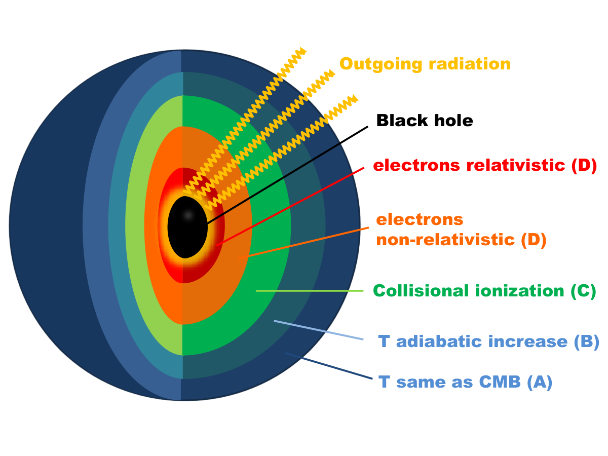
Basic equations describing the accretion in the outer region where the ionization fraction coincides with that on the cosmological background () are given by
| (82) | |||
| (83) | |||
| (84) |
where is the radial gas velocity. The last terms in the second and the third equations represent the drag force and the cooling by the CMB, respectively. From these equations, the mass accretion rate is determined. Then, the continuity equation gives the electron number density at the vicinity of the event horizon as
| (85) |
where we have used the free fall velocity . The gas temperature at the vicinity of the event horizon can be also determined by adiabatically extending the profile derived by solving the above basic equations down to the horizon. From the knowledge of the electron number density and the temperature, the luminosity of the bremsstrahlung radiation is determined as
| (86) |
where is a certain function fixed by the elementary process of the bremsstrahlung radiation. Then, the energy injection rate per volume of the radiation produced by the PBHs is given by
| (87) |
where is the average of the luminosity over the PBH peculiar velocity relative to the baryonic gas. In [166], it was assumed that the luminosity in the case where the PBH moves relative to the baryonic gas was obtained by simply adding the relative velocity to the sound speed at infinity. The injected radiation interacts with the background gas by the Compton scattering. Time evolution of the energy actually deposited to the gas is given by [166]
| (88) |
which is approximate, and derived under the assumption that most of the energy is injected near , corresponding to the characteristic temperature of the gas near the BH horizon It was assumed that the deposited energy in this manner is distributed to the increase of the gas temperature, ionization fraction, and the excitation of the hydrogen atoms (to the first excited states) as [167]
| (89) |
where . These equations describe how the temperature and the ionization history are modified by the accreting PBHs. For instance, increase of the ionization fraction enhances the CMB optical depth, which results in the damping of the small scale CMB fluctuations and the enhancement of the polarization power on large angular scales compared to the standard case. Also, the shift of the redshift of the last scattering changes the phase of the acoustic oscillations in the CMB spectrum. In [166], the modified CMB fluctuations were computed by using the recombination and the Boltzmann codes [168, 169] and they were compared with the CMB TT, TE and EE power spectra provided by the Planck collaboration [170]. The resultant constraint on the PBH abundance is shown in Fig 11.
Accretion of gas onto the PBHs in the early Universe (even before the CMB decoupling) also induces the CMB spectral distortions since the produced photons by the accreting PBHs are not completely thermalized. Photons generated in the redshift achieve the kinetic equilibrium and yield the non-vanishing chemical potential (-distortion). Here the upper and the lower limit on the redshift correspond to the temperature above which the photon-number changing process efficiently occurs to make the distribution Planckian and the temperature below which the kinetic equilibrium is no longer maintained, respectively. Photons generated in the redshift yield the Compton- distortion. Here the lower limit corresponds to the temperature at which the baryonic gas decouples from the CMB. Contrary to the meaningful constraint on by the temperature and the polarization anisotropies of CMB, it was also found in [166] that the induced amplitudes of both the and -distortions are too small to be relevant to present and future observations.
So far, the discussion has been based on the assumption that the accretion is spherical. The accretion is approximately spherical when the angular momentum of the gas at the Bondi radius is smaller than the one determined by the Keplerian orbit at the innermost stable circular orbit. If this is not satisfied, the gas motion becomes Keplerian before it is absorbed by the PBH and the accretion disk forms around the PBH. While the radiation in the case of the spherical accretion originates from the bremsstrahlung radiation, the radiation is more efficiently produced by the viscous heating in the presence of the accretion disk [140]. As a result, the radiative efficiency is typically higher for the accretion disk than the spherical accretion. In [171], it was claimed that the spherical assumption may be violated after the recombination. In this reference, based on the analytical estimation, it was suggested that the accretion disk forms around the PBH. Performing the similar analysis for the CMB temperature and the polarization anisotropies described above for the case of the accretion disk, it was found that the corresponding constraint on becomes much stronger than the one obtained in [166]. The derived constraints are shown in Fig 11.
3.3.2 X-rays and radio from the present-day PBHs
In the previous subsubsection, we have considered the gas accretion onto the PBHs in the early Universe and its effects on the CMB. PBHs in the present Universe also accrete the surrounding gas if they are in the dense environment, and the constraint on the PBH abundance can be obtained by the comparison between the observational data and the theoretical predictions of the electromagnetic waves from the accreting PBHs.
In [172], radiation spectra originating from the gas accretion onto the PBHs of in the solar neighborhood was computed based on the assumption that the accretion is modeled by the advection-dominated accretion flow (ADAF). This research was motivated by the microlensing observations that hint the PBHs of mass as dominant component of dark matter. It was found that the radiation spectra from the PBHs could be at the detectable level at the IR-optical band and is negligibly small at the X-ray band. This implies that a meaningful upper limit on the PBH abundance could be obtained from the IR-optical band only. However, since the main interest in [172] was the detectability of the PBH signal by the accretion, explicit number for the upper limit on was not given. Since there are contaminations from other astrophysical sources, for instance young stellar objects at the IR-optical band, it is important to keep in mind that it is crucial to do the consistency check over the multi-wavelength bands when one claims the positive detection of the PBHs from the accretion.
In [173], the upper limit on the PBH abundance for was obtained by using the Very Large Array (VLA) radio and the Chandra X-ray observational data. The flow of the argument is as follows. First, the PBH was assumed to accrete the surrounding gas with the mass accretion rate given by
| (90) |
where the value of , which measures the amount of mass accretion rate normalized by the Bondi accretion rate, was chosen to be , which is consistent with X-ray observations of dwarf nova and the nuclear accretion in galaxies (see also [174]). The radiative efficiency, that converts the mass accretion rate to the bolometric luminosity from the accreting gas, was then assumed to be given by
| (91) |
where is the mass accretion rate corresponding to the Eddington limit. That the radiative efficiency is proportional to the mass accretion rate for , which is the region of our current interest, is suggested by the observational data [175]. In order to obtain the X-ray luminosity out of the bolometric luminosity, a relation
| (92) |
was adopted. It is known that many accreting BHs accompany jets from which radio waves are emitted. Then, by making use of the so-called fundamental plane [176], which is an empirical relation among the mass of BH accompanying jets, X-ray luminosity , and radio luminosity , the radio luminosity was computed under the assumption that PBHs accreting the gas produce jets. With this formalism to compute and from the given PBH mass (delta function mass spectrum), the Monte Carlo simulation has been performed by distributing the positions and velocities of PBHs according to the Navarro-Frenk-White (NFW) profile [177] and the Maxwell-Boltzmann distribution, respectively, and the expected detectable number of X-ray and radio sources from the PBHs have been evaluated for the Chandra [178] and the VLA observations [179]. It was found that both X-ray and the radio observations result in meaningful constraint . These constraints are shown in Fig 11.
The PBH constraint by the present-day accretion has also been obtained in [180] by using the luminosity function of X-ray binaries derived in [181] in which 29 nearby star-forming galaxies in Chandra, Spizer, GALEX and 2MASS archives were analyzed. In [180], assuming the value in Eq. (90) and for the X-ray luminosity, and introducing the dark matter disk in galaxies which has been suggested in simulations [182, 183] to the PBH distribution, luminosity function of the X-ray sources powered by PBHs was computed and was compared with the observationally determined one given in [181]. It was found that the PBHs in the mass range a few are tightly constrained. This result is shown in Fig 11.
As just described, there are theoretical uncertainties in modeling the accretion and the emitted radiation. Yet, these studies demonstrate that the accretion to the present-day PBHs has a potential to provide a meaningful constraint on the PBH abundance. Finally, before closing this section, we mention that searching electromagnetic signals from the isolated astrophysical black holes (i. e., non-PBH) has also been a target of active research (e. g. , [172, 184, 174, 185]).
3.4 Large scale structure constraint
PBHs randomly distributing in space in the early Universe generate primordial density perturbations by their Poisson fluctuations on scales larger than the PBH mean distance, as first noticed in [186]. The mean comoving distance of PBHs is given by
| (93) |
Denoting by the comoving PBH number density, the number of PBHs in the comoving volume fluctuates typically as , where is the average PBH number in that volume. The fluctuations are isocurvature perturbations since they are present on the hypersurface where the radiation energy density looks uniform. Thus, in the presence of the PBHs, on top of the standard nearly scale-invariant adiabatic perturbations, the dark matter density contrast has the isocurvature perturbations whose variance is given by
| (94) |
on the comoving scale . The scaling of the variance as shows that the produced dark matter perturbations are more enhanced on smaller scales. Equivalently, in terms of the dimensionless power spectrum, the PBHs yield the contribution
| (95) |
for which the spectral index is 3, namely, extremely blue spectrum.
Based on this observation that the Poisson fluctuations in the PBH distribution enhance the dark matter perturbations on small scales, their impact on the Ly forest observations was investigated in [187]. The basic idea is as follows. Spectra of distant quasars and galaxies show many absorption lines known as the Ly forest. This arises due to the intervening neutral hydrogen in the intergalactic medium between the quasars and the Earth (typically ) that absorbs photons from quasars by the Ly transition ( to , where is the principal quantum number of the hydrogen atom). Although this epoch is after the reionization, there is still a tiny fraction of the neutral hydrogen in the intergalactic medium because of the balance between the photoionization by the surrounding UV radiation and the recombination and tiny amount of the neutral hydrogen is sufficient to produce the Ly forests. The wavenumber corresponding to this transition is Å. When the photons are partially absorbed by the neutral hydrogen at redshift , then the absorption line appears at in the observer frame. The optical depth of the Ly transition to the direction of a quasar is given by (e. g. , [188])
| (96) |
where is the baryon density normalized by the average value, and is the fraction of the neutral hydrogen. This equation shows that the Ly absorption is more efficient in the site where baryon is denser. Because of this, many absorption lines in the spectra, namely, fine fluctuations of for the relevant range of , reflect the inhomogeneous distribution of baryonic matter. Given that the baryon perturbations are affected by the dark matter perturbations gravitationally, statistical properties of the optical depth encode those of the dark matter perturbations. Conversely, observational analysis of the optical depth allows to probe the matter perturbations on small scales down to , where the minimum scale is determined by the thermal broading of the spectra of the Ly forest. These scales are mildly non-linear in the Ly epoch.
In [187], superposing the dark matter isocurvature perturbation given by Eq. (95) (assuming ) on the standard adiabatic perturbations, the resultant Ly clouds were computed for various PBH masses by the use of hydro-dynamical cosmological simulations. Then, the power spectrum , which is a two-point function of the Fourier transform of the transmitted flux defined by was evaluated and compared with the observational data presented in [189]. It was found that the PBHs heavier than comprising all the dark matter produce too much power of the transmitted flux and are inconsistent with the Ly observations. Although the explicit upper limit on is not provided in [187], simple analytical expression for the upper limit consistent with the results of [187] was given in [7]. The main point of [7] is that the matter perturbations sourced by Eq. (95) should not exceed , typical amplitude of the matter perturbation, at the Ly epoch, which yields
| (97) |
This constraint becomes meaningless when it implies that the PBH mean distance (93) is larger than the size of the Ly clouds . Thus, Eq. (97) makes sense when
| (98) |
is satisfied. Equivalently, Eq. (97) can be also obtained by requiring that the power spectrum of Eq. (95) at the Ly scale () is less than the value of the standard one based on the consistency between the prediction of the standard adiabatic perturbations and the observed Ly forests.
In [190], inspired by the first detection of GWs by LIGO, interesting suggestion was made that PBHs with mass comprising all the dark matter can solve the potential tension of the observed near-IR cosmic infrared background (CIB) anisotropies. CIB is accumulated emission of luminous objects throughout the history of the Universe (e. g. [191]) and was detected for the first time by COBE DIRBE instrument [192]. Intriguingly, measured anisotropies of CIB obtained by removing the foreground stars and galaxies are larger than expected and cannot be explained only by the contribution from remaining faint galaxies [193]. This potential tension basically arises due to rareness of halos where luminous stars form in high redshift. Denoting by efficiency that baryons inside each halo convert to luminous sources, the required value of to explain the observed amplitude of the CIB fluctuations is estimated as [190]
| (99) |
where we assumed that a mass-fraction of dark matter is contained in the halos that have luminous sources, and is the effective average redshift. How to achieve such high value is a challenging task if . Based on the idea explained above that the additional dark matter fluctuations sourced by the PBHs increase the minihalos in high redshift, was computed in the presence of PBHs and was found to become much larger than that in the conventional CDM case. Hence, in this scenario, the required value of is reduced to very modest one, which is the main point in [190] that PBHs can explain the CIB fluctuations.

3.5 Indirect constraints
So far, we have considered the cosmological and astrophysical effects caused by the PBHs and discussed how the PBH abundance can be constrained by them. Those constraints are direct in the sense that all the effects are directly triggered by the PBHs. A nice point of the direct constraints is that they do not resort to the formation mechanism of PBHs. Any model predicting the PBH formation must satisfy the direct constraints in order for it to be considered as a consistent model.
In addition to the direct constraints, there are indirect ones, which are the subjects of this section. As we have discussed in great detail in Sec. 2, the most popular mechanism of the PBH formation is the direct gravitational collapse of the primordial density perturbations, which can be naturally embedded in the framework of inflation in which the quantum fluctuations of the scalar fields are the ultimate origin of the primordial density perturbations. In this scenario, PBHs form only at high- (typically ) regions that are extremely rare. Although the other regions are not inhomogeneous enough to produce PBHs, they are still inhomogeneous enough to induce effects that are already excluded by or marginally consistent with observations, depending on the statistical properties of the primordial density perturbations. Those effects, which we are going to discuss in detail, are not sourced by the PBHs but by the density perturbations that seed the PBHs, and hence the resultant constraints on the PBHs are indirect. We have to keep in mind the underlying assumptions when one tries to constrain a particular inflation model predicting the PBHs by using the indirect constraints.
3.5.1 Stochastic gravitational waves from the primordial density perturbations
The first effect that the primordial density perturbations seeding the PBHs cause is the stochastic gravitational waves produced by the mode-mode coupling of the density perturbations. Density perturbations, which are classified as the scalar-type, evolve independently of the gravitational waves (GWs), which are classified as the tensor-type, at the linear order in the perturbation (e.g., [194]). This independence no longer holds beyond the linear order, and the GWs are sourced by the density perturbations at the second order by their mode-mode couplings #15#15 #15 Conversely, stochastic GWs also source the density perturbations by the mode-mode couplings. From the requirement that the resultant density perturbations do not lead to the overproduction of PBHs, upper limit on the amplitude of the stochastic GWs can be obtained [195, 196]..
Assuming that primordial density perturbations existed on super-Hubble scales, the production of the GWs by the second-order effect happens dominantly at the time when the density perturbations re-enter the Hubble horizon [197, 198]. In other words, GWs are mainly generated at the same epoch as the PBH formation. Once produced, those GWs freely propagate in the subsequent epochs and are still permeating the present Universe. Combining that typical frequency of such GWs at the formation time is comparable to the Hubble horizon and that the horizon radius at that time is comparable to the size of the PBHs allows to relate the PBH mass to the frequency of the GWs at present time as [199]
| (100) |
Thus, primordial density perturbations producing the stellar-mass PBHs generate ultra-low frequency GWs in band. Quite interestingly, those low-frequency GWs are severely constrained by the pulsar timing experiments.
Pulsars, which are rapidly rotating neutron stars emitting beam of radio waves, are useful to probe low-frequency GWs (e.g. [200]). In particular, millisecond pulsars, which rotate with period of , are observed to be significantly more stable than the normal pulsars. The arrival times of each pulse from the millisecond pulsars have been measured accurately and are compared with the predictions of the pulsar timing model. Just as the expansion of space, i.e. time-varying space-space components of the metric, causes the cosmological redshift, the pulse frequency , where is the time interval between the arrival times of the successive pulses, is modulated if GWs are present. The modulation of the pulse frequency is given by [201]
| (101) |
where is a geometrical factor depending on the propagation direction of the GWs relative to the direction of the pulsar, represent GWs, is the distance to the pulsar, and and is position of the Earth and the pulsar, respectively. This induces the timing residuals of the pulse arrival time at time (with reference to time ) as
| (102) |
A few hundred of millisecond pulsars have been observed. It is reasonable to think that the timing residuals caused by the GWs (102) for the pulsars are strongly correlated since the frequency modulations due to the first term in Eq. (101) become almost identical. It was shown by Hellings and Downs [202] that the correlation function (normalized by the GW amplitude) of the timing residuals by the stochastic GWs between the pulsars separated by the sky angle is given by
| (103) |
By searching this type of correlation in the measured data for many pulsar pairs, which is known as the pulsar timing array (PTA) experiment, GWs can be detected if they exist by amount more than the sensitivity the experiments can reach. Otherwise, the upper limit on the abundance of GWs is obtained.
Currently, there are three major PTA projects, the Parkes Pulsar Timing Array (PPTA) [203], the North American Nanohertz Observatory for Gravitational Waves (NANOGrav) [204], and the European Pulsar Timing Array (EPTA) [205], that aim to detect the ultra-low frequency GWs in the range. So far, no detection of the stochastic GWs has been reported, and the upper limit on the GWs has been derived.
Now, let us return to the theoretical computations of the secondary GWs produced by the primordial density perturbations. First, let us write the metric representing the scalar-type perturbations and the sourced tensor-type perturbations on the flat FLRW spacetime [197, 198];
| (104) |
where and are scalar-type perturbations (gravitational potential and curvature perturbation, respectively) and are the tensor-type perturbations satisfying the transverse and traceless conditions , where . In the absence of the anisotropic stress, which is a good approximation [198], we have . Here, we do not include generated during or after inflation by some other mechanisms since they do not affect the GWs we are interested in in this section. The evolution of at the linear order in the radiation dominated era is given by
| (105) |
The solution of this equation in the Fourier space with the requirement of vanishing decaying mode is given by
| (106) |
where the initial condition is fixed either by the assumed inflation model or by the assumed power spectrum of . The evolution of is also obtained by expanding the Einstein equations. At the second-order in the scalar-type perturbations, we have [197, 198]
| (107) |
where , is a projection operator that produces the transverse and traceless quantity, and the source term consisting of the products of scalar-type perturbations is given by
| (108) |
GWs can be Fourier-transformed as
| (109) |
where are polarization tensors normalized by . Knowing the time evolution of by Eq. (106), the time evolution of is determined as
| (110) |
where is the Green’s function of Eq. (107) and is a Fourier transform of the right-hand side of Eq. (107) [100],
| (111) |
where
| (112) |
The perturbations being stochastic, the induced GWs are also stochastic. A useful quantity parameterizing the amount of GWs is , the energy density of GWs per logarithmic frequency normalized by the critical density. Using the formula of the GW energy density [206]
| (113) |
and the definition of the GW power spectrum
| (114) |
we have
| (115) |
with . Then, assuming the Gaussianity of the scalar-type perturbations, for which we can decompose the power spectrum of into the product of the power spectrum of , can be written as
| (116) |
Except for , all the functions such as and are known. By using this equation, we can compute from the power spectrum of the scalar-type perturbations .
Then, assuming the delta-function type power spectrum for and its amplitude to the one predicting sizable amount of PBHs in the present Universe, it was claimed that the resultant conflicts with the upper limit set by the pulsar timing experiments [199]. The analysis was then generalized in [207] to the case where has a silk hat type spectrum with a finite width. It was found that the predicted becomes smaller for larger width (see also [208]). In [100, 209], computations of for some concrete inflation models predicting the PBHs were performed and comparison with the data of the three PTA experiments (EPTA [210], PPTA [211], and NANOGrav [212]) were made (see also [106]). Although not all the regions in the parameter space of inflation models are excluded, it was shown that pulsar timing places stringent constraints on inflation models.
So far, the primordial density perturbations sourcing the stochastic GWs have been assumed to be Gaussian. In [213], it was suggested that the constraints mentioned above can weaken for the non-Gaussian density perturbations, which may be typical when the amplitude of the density perturbation is significantly large. A basic observation behind this conclusion is that the variance of the density perturbation, which determines the magnitude of , can be smaller in the non-Gaussian perturbation than in the Gaussian case for a fixed PBH abundance. In [213], two different types of non-Gaussian density perturbations were considered. The first one is specified by the probability density function of the curvature perturbation smoothed over the Hubble horizon at the time of the PBH formation, which is given by
| (117) |
where and are free parameters. When , the perturbations are Gaussian. As explained in Sec. 2.3, the PBH fraction at the formation time is given by the probability that the perturbation exceeds the formation threshold ,
| (118) |
For fixed , the variance of becomes smaller than the Gaussian case for [214]. The second example is the local-type non-Gaussian perturbation for which the smoothed curvature perturbation in the position space is written as
| (119) |
where is Gaussian, and is a free parameter that parametrizes the significance of the non-Gaussian contribution. For positive , the variance of is suppressed than the Gaussian case [215]. According to the analysis in [213], the PTA constraint can be safely evaded if or (precise value depends on the theoretical uncertainties about the PBH formation). Similar conclusion has been obtained in [216], where the curvature perturbation obeying the statistics, motivated by the rolling axion scenario [217], was considered.
3.5.2 CMB spectral distortions from the primordial density perturbations
The second indirect constraint can be obtained from the generation of the CMB spectral distortion of the primordial density perturbations [218, 219]. The basic argument is as follows.
The perturbations of photons and baryonic gas that re-entered the Hubble horizon prior to the CMB decoupling undergo the acoustic oscillations due to the tight coupling between photons and baryons. These oscillations are eventually erased by the photon diffusion, i.e. imperfect coupling between photons and free electrons, known as the Silk damping. Using the photon mean free path , where is the number density of free electrons, and that the diffusion is described by random walks, the comoving wavenumber of a perturbation is related to the damping time of the perturbation as [220]
| (120) |
This shows that the Silk damping occurs earlier for smaller scale perturbations. Through the damping, the oscillation energy of the perturbations is transfered to the background homogeneous plasma gas. As briefly discussed in 3.3.1, if the Silk damping occurs before , the photon-number changing interactions occur frequently and the injected energy is completely consumed for the thermalization. As a result, the net effect is just the slight increase of the entropy per unit comoving volume. If the perturbations undergo the Silk damping after that redshift but before , only the kinetic equilibrium is achieved. As a result, the photons acquire chemical potential and the distribution of photons becomes the Bose-Einstein distribution (-type). Using the above equation (120), the interval of wavenumber of perturbations that yield the -type distortion is . If the perturbations dissipate after , even the kinetic equilibrium is no longer reached, and the distribution of photons is characterized by the Compton- parameter (-type). Thus, the perturbations of smaller comoving wavenumber than generate the -type distortion in the CMB spectrum.
Now, let us consider for simplicity the delta-function power spectrum of the density perturbation at with total power . To produce PBHs, is required. Then, the produced -type distortion is given by [221, 222]
| (121) |
So far, spectral distortion of the CMB has not been detected, and the strongest upper limit is placed by the COBE/FIRAS experiment as [223]. Using this limit and the fiducial value , the level of the produced -distortion (121) is inconsistent with the COBE/FIRAS bound for . This interval is only logarithmically sensitive to the choice of . In terms of the PBH mass, non-detection of the -type distortion excludes PBHs in the mass range
| (122) |
if PBHs are produced from the direct collapse of the nearly Gaussian primordial density perturbations [222] (see also [224]).
In [214], it was pointed out that the above conclusion that the PBHs in the mass range (122) are excluded can in principle be circumvented if the primordial density perturbations are strongly non-Gaussian such that amplitude of the density perturbations in all regions other than the sites of PBH formation is too tiny to induce sizable -distortion. Such a situation can be realized if only patches that later convert into PBHs experience different expansion history during inflation (see Fig. 3 of [214]).
3.5.3 Big-bang nucleosynthesis
From the last discussion in 3.5.2, it may appear that it is impossible to constrain the amplitude of the primordial perturbation for , translating to , since the Silk damping of such small scale perturbations does not leave any spectral feature in the CMB. Yet, big-bang nucleosynthesis (BBN) has a potential to exclude smaller PBHs than the above mass.
Primordial density perturbations in the range dissipate by the Silk damping in the redshift range , which is after the BBN era but much before the decoupling time of the CMB (perturbations with dissipate prior to the neutrino decoupling due to the neutrino diffusion). Injected energy by the Silk damping of those perturbations results in the increase of the temperature of the plasma gas. Because of the conservation of the baryon number, only the photon number density is increased by this process. In other words, the baryon-to-photon ratio defined by the ratio between the two number density as decreases through the Silk damping. This means that during BBN era is bigger than that in the CMB era, namely . Abundance of light elements produced by BBN is controlled by , and the measurement of the light elements in the present Universe can determine . Acoustic peaks in the CMB temperature power spectrum is controlled by , and the measurement of the CMB anisotropies can determine . The difference between and depends on how much energy was injected by the Silk damping, i.e. the amplitude of the primordial density perturbations. Therefore, the determination of and by independent observations constrains the amplitude of the primordial density perturbations in the relevant length scale [225]. From observations, we have and [226]. Using these values, the upper limit on the total power for the delta-function type perturbation was obtained as [225]
| (123) |
In [227], more stringent upper limit on was obtained by investigating the freezeout neutron fraction during BBN in the presence of the (adiabatic) primordial density perturbations (see also [228]). Those density perturbations, which dissipate after BBN, produce local temperature fluctuations during BBN since . In local regions where the temperature is higher than the average, interactions persist longer and the freezeout is delayed, resulting in smaller amount of neutrons. On the other hand, more neutrons remain in colder regions. Because of two enhancement effects in hotter regions that more baryons are available () and that physical volume is also enlarged by the metric perturbation compared to colder regions for fixed comoving volume, the averaged neutron fraction is biased toward the higher temperature region. As a result, the predicted helium abundance becomes smaller than the standard case. The derived upper limit on is [227]
| (124) |
Although this value does not immediately exclude the production of PBHs, this falls into the typical power required for PBHs. This suggests that reduction of errors in future measurements may find a PBH signal or eventually rule out the PBHs in the relevant mass range.
3.6 Future constraints
So far, all the constraints we have discussed are established constraints in the sense that they are obtained by the existing observational data. Thus, as long as the data and theory translating to the constraint are correct, the derived constraint is real and must be taken into account when one tests any early Universe model predicting the PBH formation.
In the future, those constraints will be improved by the new experimental apparatus similar to what is existing/existed but with better sensitivity. Furthermore, appearance of new technology will enable us to probe PBHs by using completely new methods. In this section, we briefly review several proposals to probe PBHs by future experiments.
3.6.1 Fast radio bursts
Fast radio bursts (FRBs) are radio transients that last only for [229]. Since its discovery in 2007 [229], many FRBs have been detected. The measured values of dispersion measures suggest that FRBs occur at cosmological distances [230]. The origin of FRBs is not known yet.
In [231], it was pointed out that lensing of the FRB signals by the intervening PBHs can be used to probe PBHs with . The idea is as follows. Gravitational lensing causes appearance of two source images. Although the angular separation of the two images is too small to be resolved experimentally, the difference of arrival times of the images becomes the order of
| (125) |
for (see Eq. (60)). Thus, PBHs heavier than produce double bursts separated longer than the burst width, hence can in principle be resolved. Considering the two redshift distributions of FRBs, constant comoving number density and the one that follows the star formation rate, the lensing optical depth has been evaluated in [231]. It was found that planned experiment the Canadian Hydrogen Intensity Mapping Experiment (CHIME), which is expected to measure FRBs per year [232], may detect tens of double bursts caused by PBHs if PBHs comprise all the dark matter and provide constraint if no such events are detected.
3.6.2 Pulsar timing array (PTA) experiments
As explained in 3.5.1, primordial density perturbations that generated PBHs from high- peaks also produce the stochastic GWs by the mode-mode coupling. The present frequency of the GWs corresponding to the PBHs in the stellar mass range is in the range which PTA experiments are sensitive to. Square Kilometer Array (SKA) is a planned giant radio telescope consisting of thousands of receptors with total collecting area being about one square kilometer . With better sensitivity, SKA is expected to detect more pulsars and improve the constraint on by orders of magnitude stronger than the current limit if no GWs are detected [233]. Such constraint, if achieved, will further tighten the constraint in 3.5.1 much more severely.
While the above constraint is indirect in the sense that the constraint is derived by looking at the GWs from the primordial density perturbations that failed to turn into PBHs, pulsar timing also has a potential to give a direct constraint on PBH abundance by measuring the effect of the Shapiro time delay caused by the PBHs intervening between pulsars and the Earth [234]. A PBH moving relative to the line of sight produces non-stationary change of the arrival times of pulses as
| (126) |
for the -th pulse [234]. Here are the observed pulse period, its time derivative, (constant) velocity of the PBH toward the line of sight, and the distance between the PBH and the line of sight, respectively. The observable effect of the PBH appears at term. According to [234], non-detection of such effect in the long term observations ( years) of known pulsars or pulsars that would be newly detected by SKA can constrain PBHs as .
3.6.3 21cm
SKA is also expected to detect cosmological 21cm line from neutral hydrogen in the dark age before reionization. Observations of such 21cm line have a potential to constrain PBHs.
21cm line is radiation emitted/absorbed by the transition between the two levels in the hydrogen 1s ground states. Energy of the spin singlet state is lower than that of the spin triplet states by . Relative number density between singlet () and triplet () hydrogen atoms is parametrized by the spin temperature as
| (127) |
There are three ingredients to determine the spin temperature as
| (128) |
where the second and the third term in the numerator represents the Lyman- pumping, namely 21cm transition through ambient Lyman- photons as singlet/triplet 2p singlet/triplet, and the collisions among hydrogen atoms, respectively [235]. The 21cm intensity is normally expressed in terms of the brightness temperature . With reference to the CMB brightness temperature, the differential temperature measured at the Earth is given by
| (129) |
where is the optical depth for the 21cm photons [235].
In [236], the effect of X-rays emitted by the accreting PBHs on the 21cm fluctuations has been investigated. Radiation emitted from the accreting PBHs in the dark age ionizes and heats the surrounding neutral hydrogen gas. Ionization reduces the amount of neutral hydrogen, Lyman- photons from PBHs affects the spin temperature through the term, and the heating of neutral hydrogen by emanating radiation also affects the spin temperature by changing the kinetic temperature . Assuming radiation intensity corresponding to of the Eddington luminosity with a power-law X-ray spectrum, brightness temperature fluctuations was computed. It was found that with SKA-like experiments upper limit on PBH will be at and at for .
In [237], based on the observation discussed in 3.4 that the random distribution of PBHs adds isocurvature component on top of the adiabatic perturbations, formation of minihalos sourced by the PBHs and their effect on 21cm fluctuations has been studied. Minihalos can change the 21cm signals since the gas temperature and the density of neutral hydrogen inside the minihalos differ from the background values. According to the analysis in [237], the PBHs with leave enhancement of the brightness temperature that is detectable for SKA for .
3.7 Constraints for the extended PBH mass function
So far, we have assumed that the PBH mass function is monochromatic, e.g., all the PBHs have the same mass. Thus, the derived constraints are valid only when the PBH mass function is sufficiently narrow, and can no longer be trusted when the mass function is broad. In this subsection, we briefly mention how to generalize the constraint on the PBH abundance to the case of the extended PBH mass function (see [8, 238, 9] for more details).
A simple formalism for deriving the PBH constraint for the extended mass function was given in [9]. Let be the PBH mass function and consider an observable which PBHs produce or contribute. Only in this subsection, we define the normalization of the PBH mass function as
| (130) |
The quantity depends on the details of experiments as well as the astrophysical phenomena one is interested in. For instance, in the microlensing experiment, is the expected number of the microlensing events detected by a particular experiment and depends on the sensitivity of the detectors. Generally, is a functional of the mass function and can be expressed as
| (131) |
where are higher order terms in . Here represents any contribution other than from PBHs. For the microlensing experiments, , the total expected number of the microlensing events during the observation period, contains only the -term as the PBH contribution, which is given by [239, 238]
| (132) |
where is the number of stars multiplied with the observation period, is the maximum (see Eq. (49)) below which the microlensing magnification becomes greater than the threshold, is the circular velocity of the Sun, and is the probability that the detector detects the microlensing events that last for the period . As we will see in the next section, if is the merger event rate of the PBH binaries that are formed in the early Universe, the expansion (131) starts at the term if only the third BH is taken into account as the dominant source of the tidal force and starts at even higher-order terms if more distant PBHs are also included. On the other hand, for PBH binaries that are formed in the low-redshift Universe by the close encounters, is given by the -term. These examples show that the order in at which the expansion of (131) starts varies for different observables.
Let us consider the simplest case where is dominantly given by the term. Suppose the observations place an upper bound on as
| (133) |
Then, for the monochromatic mass function , the above constraint becomes
| (134) |
where is the maximally allowed value of by the observation under consideration when all the PBHs have mass . Replacing by , we finally obtain
| (135) |
This formula enables us to derive the constraint on the extended mass function once we know the upper limit for the monochromatic mass function. This simple conversion does not hold in general when higher order terms contribute to .
In [9], based on the above formalism, the constraints on the PBH abundance for several types of the extended mass function were obtained. The results show that the constraints generally become stringent for the extended mass function compared to the case of the monochromatic mass function due to the combination of the multiple observational limits for different PBH masses.
4 PBHs as sources of gravitational waves (GWs)
As we have discussed in detail in Sec. 3, before the direct detection of GWs by LIGO, searching for the PBHs in the Universe to a varying degree relied on the electromagnetic waves. For instance, gravitational lensing uses the background electromagnetic sources such as stars and quasars, and the dynamical constraints are derived by the observations of stars which PBHs affect. So far, although there are a couple of studies which attributed some unexplained observational signals to the PBHs, no observational searches for PBHs by the electromagnetic waves have detected inarguable evidence for the existence of PBHs.
Direct detection of GWs by the laser-interferometers is a completely novel method to search for PBHs that does not rely on the electromagnetic waves. Soon after LIGO announced the first detection of GWs in February 2016, which are caused by the merger of two BHs in a binary, several groups pointed out the possibility of the scenario that the observed BHs are PBHs [12, 13, 14, 190]. Thus, exciting possibility has arisen that we might have discovered PBHs for the first time by the direct observation of GWs (not just constraint!).
Explaining the LIGO event by the PBHs is not trivial in two aspects. First, since the GWs are emitted from the BH binaries, formation mechanism of the PBH binary must be considered in order to test the PBH scenario with GW observations. Secondly, as discussed in Sec. 3, there are existing constraints on the PBH abundance for the mass around the observed BH mass . It needs to be checked if the PBH scenario does not conflict with those constraints. These issues, which we will address in detail later, are the first main topic in this section. It will turn out that those issues are cleared and the PBH scenario can be considered as a reasonable candidate scenario for the observed BH merger event.
There are also astrophysical explanations for the observed heavy stellar-mass BHs (see [11] and references therein): isolated field binary scenario in which two stars in an isolated binary collapse to BHs in decreasing order of star mass, and dynamical formation scenario in which isolated BHs in dense stellar environment form BH binaries at the core and eventually are ejected by the three-body interactions. In both cases, studies [240, 241, 242] suggest that heavy BHs about are born out of stars with low metallicity (at most half of solar-metallicity) . Although there are many astrophysically uncertain factors in estimating the merger event rate, these scenarios are roughly consistent with the GW observations. Thus, our next task is to clarify how to discriminate those scenarios of the binary BHs and to pin down the correct one.
The GW astronomy has just began, and its future is bright. In the coming decade, the sensitivity of the existing GW experiments will greatly improve and many merger events of the BH binaries will be detected. Looking at further future, new detectors with a larger armlength will be build both on ground and in space, which can probe GWs in different frequency bands. By those experiments, we will obtain much information of BH binaries such as mass distribution, space distribution, redshift distribution and spin distribution. These information will definitely help us discriminate different scenarios of the binary BHs. How such information can be used for this purpose is the second topic in this section. Concerning this point, discussions about the astrophysical scenarios are beyond the scope of this monograph and we will concentrate on the PBH scenario in what follows.
4.1 Formation of PBH binaries
Here, we will briefly review two distinct formation mechanisms of the PBH binaries. It is important to remark here that the two mechanisms are not incompatible, i.e., not like the relationship between oil and water, but operate at different epoch in the cosmic history. Thus, what matters is to figure out which mechanism is more efficient to make PBH binaries that merge by present time.
4.1.1 PBH binary formation in the early Universe
The first mechanism we are going to discuss operates in the epoch when the Universe was dominated by radiation. This mechanism was proposed in [15] to investigate the detectability of binary mergers of MACHO PBHs (). In [15], it was assumed that , all the PBHs have the same mass, and PBHs are initially distributed randomly in space (Poisson distribution). In the following, we consider the monochromatic PBH mass function and uniform distribution of PBHs and treat as a free parameter.
Just after the PBHs were formed in the very early Universe, they were distributed sparsely in space, that is, mean distance at that time is much longer than the Hubble horizon. Because of the rapid cosmic expansion, they are on the expansion flow and the mean distance grows in proportion to the scale factor . Since the Hubble horizon grows as , the mean distance relative to the Hubble horizon decreases as the Universe expands. Denoting by the mean PBH distance at redshift , its length normalized by the Hubble horizon is given by
| (136) |
for , where is the redshift of the matter-radiation equality and is the comoving (initial) PBH number density. Thus, for the stellar-mass PBHs, unless is extremely tiny as , there is period in the radiation dominated epoch in which there are typically more than one PBHs in the Hubble horizon. Range of of our interest is much larger than this value.
Let us focus on a PBH and the PBH closest to it, and let their comoving distance be . The physical separation at redshift is then . The cosmic expansion acts as a force that pulls two PBHs away from each other. Two PBHs are also pulled by the gravitational force acting between them. The corresponding free-fall time becomes shorter than the Hubble time at a certain time during the radiation dominated epoch if the comoving distance is shorter than
| (137) |
PBH pair satisfying this condition decouples from the cosmic expansion and becomes gravitationally bound #16#16 #16 This picture has been confirmed to be correct by numerically solving the Newtonian equations of motion [243, 244].. Conversely, PBH pair with comoving distance longer than never becomes gravitationally bound since a ratio of the free-fall time to the Hubble time remains constant in the subsequent matter dominated epoch. The decoupling redshift is given by
| (138) |

During the two PBHs come closer, the surrounding PBHs, especially the nearest one, exert torques on the bound system. As a result, the two PBHs avoid a head-on collision and form typically a highly eccentric binary (see Fig. 12). The major axis of the binary orbit is equal to . The angular momentum of the binary is estimated by multiplying the exerted torque from the nearest PBH by the free-fall time and is given by
| (139) |
where is the comoving distance to the nearest PBH and a factor of has been ignored. Assuming the Keplerian motion after forming the binary, the angular momentum is related to the eccentricity of the orbit as , where and is the reduced mass and total mass. We can convert these equations in terms of and as
| (140) |
Because of the random distribution of PBHs, the probability that comoving distances are in the intervals and is given by
| (141) |
Instead of dealing with this probability distribution, the simplified one as
| (142) |
was used in [15]. Notice that because of , there is an upper limit on the eccentricity for fixed (and hence for fixed ) as
| (143) |
Schematic graph of as a function of is shown in Fig. 13 as a blue curve. Notice that there is also a maximum for as .
Knowing the probability distribution of , we can translate it in terms of by using the formula (140) as
| (144) |
This equation tells us how much PBH binaries with orbital parameters in , exist in the Universe at formation time #17#17 #17 It is worth mentioning that exact distribution function of the initial angular momentum taking into account all the distant PBHs was obtained in [244].. After PBH binaries were formed in the radiation dominated epoch, each PBH binary continuously emit gravitational waves and finally merge much later. The estimate of the merger rate will be discussed in the subsequent subsection.
4.1.2 PBH binary formation in the present Universe
In addition to the PBH binary formation in the radiation dominated epoch, PBHs can form binaries in the present Universe, which we review in this subsection.
Let us consider a situation where a PBH traveling in space accidentally has a near-miss with another PBH. These PBHs may be concentrated in local region like inside larger dark matter halo or simply moving freely in space. For the moment, we do not make a particular assumption on how PBHs are distributed in the region of our interest. Fig. 14 shows a schematic picture of the close encounter with impact parameter and periastron . Near the periastron, relative acceleration of the PBHs becomes the largest and dominant emission of gravitational radiation occurs. If the amount of energy of the emitted GWs is greater than the kinetic energy of PBHs, then the PBHs cannot escape to infinity any more and form the bound system. Since the direct head-on collision is probabilistically unlikely, the binary typically results.
Let us investigate this problem more quantitatively [245]. We assume that the power of GWs is estimated by the unperturbed trajectory (without backreaction due to GW emission) in the Newtonian approximation. According to Peters [246], the time-averaged energy loss rate of the binary in the Keplerian orbit due to gravitational radiation is given by
| (145) |
Thus, the energy loss during one orbital period becomes
| (146) |
where we have used the Kepler’s third law and . We can approximate the trajectory of the close encounter by the ellipse with since the true trajectory is physically indistinguishable from the ellipse near the periastron where the dominant emission of GWs occurs. Then, the energy loss by the close-encounter is obtained by plugging into the above equation,
| (147) |
If this energy is greater than the kinetic energy , where is the reduced mass and is the relative velocity at large separation, then the PBHs form a binary. This imposes a condition on as
| (148) |
In the Newtonian approximation, relation between and is given by
| (149) |
The encounter with the impact parameter less than yields a binary. In the limit of the strong gravitational focusing (), which we are interested in, the cross section for forming a binary becomes
| (150) |
Contrary to the PBH binaries that are formed in the radiation dominated epoch, the PBH binaries produced by the present mechanism merge in less than the age of the Universe [247].
4.2 Merger event rate of PBH binaries
Having explained two mechanisms of the formation of PBH binaries, we review the expected merger event rate of PBH binaries formed in each mechanism, separately.
4.2.1 PBH binaries formed in the early Universe
The following discussion is based on [14]. PBH binaries that are formed in the radiation dominated epoch continuously emit gravitational waves, gradually shrink, and finally merge. Since the initial orbital parameters of the binaries are stochastic, some binaries merge in the past, some other at present epoch, and the others in the future. According to Peters [246], a binary consisting of point masses and with orbital parameter merges due to gravitational radiation after time given by
| (151) |
The lower limit of integral is set to by the assumption that the binary is almost circular () just before the binary merges. Because of the smallness of the tidal force from the outer PBHs compared to the gravitational force between the PBHs that form the binary, the orbital eccentricity at the binary formation time is typically close to unity. When , the above formula can be simplified as
| (152) |
This shows that highly eccentric binary merges in shorter time by a factor than the circular binary with the same semi-major axis, which simply reflects that the binary radiates GWs dominantly around the periastron. It is this factor that makes PBHs binaries formed in the radiation dominated epoch efficiently merge in the age of the Universe and yields the merger event rate that can even exceed the one estimated by LIGO when PBHs comprise all the dark matter.
For simplicity, let us consider the case where all the PBHs have the same mass. In this case, Eq. (152) becomes
| (153) |
From this equation, we can express as a function of and as . Then, we can rewrite the probability (144) as
| (154) |
Since the observations do not measure the initial eccentricity of the binaries, we integrate this probability over along the curve up to either a point where the line intersects the curve or a point where the line intersects the line , whichever comes first (see Fig. 13). Plugging and integrating over , we find
| (155) |
where is defined by
| (156) |
and is defined by . This gives the probability that a given PBH forms a binary and merges at a time in . Thus, the merger event rate per unit volume per unit time (at time ) is given by
| (157) |
The red curve in Fig. 15 shows for , BH mass close to the first event (GW150914) detected by LIGO, and for as a function of . We find that the merger rate largely exceeds the LIGO’s observation when and lies in the band estimated by LIGO for . Thus, in the present mechanism of the PBH binary formation, the case that PBHs constitute only a fraction of dark matter is observationally relevant.
The knee at corresponds to the bifurcation point . Physically, this bifurcation can be understood as follows. Since there is an upper limit on the distance between neighboring PBHs that form binary, Eq. (153) tells that there is also an upper limit on the eccentricity for fixed . Since the eccentricity is caused by the tidal force from the outer BH, the eccentricity becomes closer to unity as the outer BH is more separated. Probability of the location of the outer BH peaks at the mean separation of PBHs. If falls below about , the eccentricity caused by the outer BH at the mean separation exceeds the mentioned upper limit on the eccentricity and the outer BH must be located closer than the mean distance to cause the merger at time . As a result, the merger rate is suppressed by the volume factor than the case where the outer BH is at the mean distance, which produces the knee.
One may wonder if the mergers of PBH binaries that have accumulated over the age of the Universe significantly modify the PBH mass function in the present Universe. Fig. 16 shows the probability, which is obtained by integrating Eq. (157) over the cosmic time up to , that any PBH undergoes a merger by the time . From this figure, we find that even in the case with the probability that a PBH has merged by the present time is about . Thus, in this case the PBH mass function in the present universe is reduced by at and has a little spike at . For smaller , the time evolution of the mass function is more moderate.
From the accumulated merger probability given in Fig. 16, we can also estimate the accumulated merger rate per unit time as for , and yr. Thus, the typical time interval between the successive merger events that occurred in the Hubble volume is much longer than the duration of a single merger event, which is classified as the ”shot noise” type according to Ref. [249].
We have assumed that PBHs are not clustered initially. The effect of clustering on the merger rate (157) was addressed in [250]. According to their result, the merger rate is enhanced by the clustering, which is a natural consequence since the clustering effectively increases the PBH comoving number density.
There are several effects that have been ignored in deriving the merger rate (157). These include tidal force from the outer PBHs other than the nearest one, subsequent capture of the outer BH by the already formed binaries, initial peculiar velocities of PBHs, gravitational perturbation by the surrounding non-PBH dark matter inhomogeneities, subsequent accretion of dark matter and baryonic gas onto the PBH binaries.
The first three effects have been investigated in [243] in which was assumed. Because the tidal force is inversely proportional to the distance cubed and each outer PBH exerts torque to random direction, only a few outer PBHs mostly contribute to the tidal force. As a result, the merger event is reduced by at most . The present mechanism of the formation of the bound system by the decoupling from the cosmic expansion works as long as the distance between PBHs is smaller than (see Eq. (137)). For , becomes the mean PBH distance. This means that the outer PBH, which generated angular momentum of the inner PBH binary, is commonly trapped by the binary later, resulting in the hierarchical triple system. As the three-body problem is difficult to analyze, fate of such triple system is hard to predict. In [243], such a case was left aside and another case that the distance to the nearest outer PBH is greater than was investigated. Restricting the PBH mergers to the latter case, it was found that the merger rate is reduced by about , which is not a significant impact. If , which is the case relevant to LIGO observation, we expect that the probability of forming the triple system is more suppressed than the case of since the fraction of PBHs satisfying the condition Eq. (137) is reduced by a factor . Initial peculiar velocities, that are randomly directed for each PBH, naturally yields angular momentum of the binary. If the angular momentum from the peculiar velocity is larger than the one from the tidal force we discussed, the prediction of the merger rate will be modified. According to [243], the effect of the peculiar velocity is to reduce the merger rate by at most even if the initial peculiar velocity is equal to the speed of light.
In [251], the additional tidal force from the adiabatic perturbation of non-PBH dark matter (valid for ) was taken into account and its effect on the merger rate was investigated. Since we do not know the power of dark matter perturbations on relevant scales, smaller than the ones probed directly by the CMB observations, straightforward extrapolation of the Planck results was adopted to define the dark matter perturbations. It was found that the inclusion of this effect reduces the merger rate by at most a factor of . Effects of the tidal force from the non-linear structures of dark matter on the PBH binaries have been estimated in [244] and were found to be insignificant as well.
The accretion of dark matter and baryonic gas onto the PBH binaries was investigated in [252]. According to this study, the continuous accumulation of matter onto the binaries can rapidly decrease the binary radius by the dynamical friction and the merger may happen in the early Universe. More recent study in [244], based on the simple analytic calculation, suggests that the baryonic mass accumulated around the PBHs is likely overestimated in [252] and the baryonic effect is not significant enough to change the evolution of the PBH binaries. Yet, more detailed studies are needed to clarify the effectiveness of this scenario.
4.2.2 PBH binaries formed in the present Universe
The merger event rate of PBH binaries formed in the present Universe was estimated in [12]. The cross section of forming PBH binaries by the close encounter given by Eq. (150) shows that the binary formation is effective for low relative velocity. The encounters, which are accidental, are more frequent in high density region than the low density region. These facts suggest that the PBH binary formation occurs efficiently inside the low-mass dark halos, which are dense and have small virial velocity. The merger rate inside a halo with mass is given by
| (158) |
where is density profile of PBHs inside the halo, and denotes the average over relative velocity distribution with given by Eq. (150). In [12], it was assumed that and the velocity distribution is given by the Navarro-Frenk-White profile and the Maxwell-Boltzmann distribution, respectively. Then, the total merger rate per unit volume and unit time is given by
| (159) |
where is the halo mass function and is the minimum mass of halos that have not yet evaporated by the present time. Three different mass functions, one obtained by the Press-Schechter formalism, one based on the simulations by Tinker et al. [253], and the other that has cutoff at small mass from Jenkins et al. [254], were employed in computing . The result for is given by
| (160) |
where for the Press-Schechter, Tinker et al., and Jenkins et al., respectively.
The blue curve in Fig. 15 shows given by Eq. (160) with . We find that the expected merger rate is consistent with the LIGO observation when . The fact that there is a physically interesting region consistent with the observations by LIGO makes the binary formation path by the present mechanism interesting. This formation path becomes important if the mergers of PBH binaries formed in the radiation dominated epoch are significantly reduced by some mechanism.
If PBHs cluster in the vicinity of the supermassive BHs at galactic centers, they can efficiently form binaries by the close encounter mechanism [255]. According to the study in [255], the expected merger rate exceeds the one given by Eq. (160) for some possible range of the slope of the PBH density profile around the supermassive BHs. In such a case, PBHs in the galactic center may become the dominant channel to form binaries which emit GWs.
4.3 Constraint on the PBH abundance from the GW observations
In the previous subsection, we have seen that PBH binaries that are formed in the radiation dominated era merge with frequency consistent with the one estimated by the LIGO observations if and merge much more frequently if . This means we can use the GW observations to place an upper limit on irrespective of whether the observed mergers of BH binaries are attributed to PBHs or not. This was done in [244] for various PBH masses with the monochromatic mass function. The derived constraint is shown in Fig 17. We see that the derived constraint excludes stellar mass PBHs as the dominant component of dark matter. This result demonstrates that GWs observations provide a novel tool to probe/constrain PBHs independently of the electromagnetic observations.
4.4 Distinguishing from other scenarios
In the previous subsections, we have reviewed the two mechanisms of the PBH binary formation that work at different cosmic epochs and discussed that the LIGO events can be explained by the mergers of the PBH binaries. Of course, the PBH scenario is not the only explanation of the LIGO events and there are several astrophysical scenarios that have been proposed as the origin of the LIGO events. So far, due to the small number of the detected events, those scenarios are allowed observationally. The next obvious task is to clarify how we can test the PBH scenario and discriminate it from the others by using the future observations that will bring much more information. This is the main topic of this subsection.
4.4.1 Stochastic GW background from PBH binaries
At the time of writing this article (autumn 2017), LIGO has detected five GW-events from BH-BH mergers. These GW-events were close enough so that they were heard as single events by the detectors. In addition to these loud events, there are other merger events that occur at more distant places. Although GWs from such mergers pass through the Earth more frequently than the louder ones, they are tiny, buried in noise, and may not be identified as single events. Yet, those events may be detected as a whole by taking correlations of the GW signals among different detectors and integrating it over some time. If such tiny GWs exist, after the time integration, the GW signal will emerge. Such GWs are referred to as stochastic GW background.
It is customary to represent the strength of the stochastic GWs in terms of the GW energy density per logarithmic frequency bin normalized by the critical density (for instance [256]);
| (161) |
For GWs that are emitted by the mergers of compact objects in binaries, can be written as [257]
| (162) |
where is the merger rate of the source we are interested in, and is the spectral energy density of a source, which describes how much energy is released from the source in the form of GWs with frequency . The spectral energy density can be determined by general relativity. Based on the phenomenological waveforms in the Fourier domain for the inspiral, merger, and ringdown phases for non-spinning BH binaries [258], Zhu et al. [259] converted it to the spectral energy density as
| (163) |
where is the chirp mass and are fitting parameters. Schematic shape of this function is shown in Fig. 18. Modified waveforms for BH-BH binaries, generalized to non-precessing spins, are given in Ajith et al. [260].
For the evaluation of from the mergers of PBH binaries, we use either Eq. (157) or (160) for in Eq. (162). For the PBH binaries formed in the radiation dominated epoch, the expected was computed for the first time in [261] for MACHO mass range . In light of the detection of BH-BH binaries of by LIGO, the computation of for was done in [262]. The analysis was generalized to the case where the PBH mass function is not monochromatic in [250]. For the PBH binaries formed in the present Universe, the expected was computed in [263] (assuming monochromatic PBH mass function). Fig. 19 shows curves of predicted in the aforementioned PBH scenarios, red curves for PBH binaries formed in the radiation dominated epoch (, and ) and blue one for PBH binaries formed in the present Universe ( and ). As is anticipated from Fig. 15, PBH binaries formed in the radiation dominated epoch produce larger stochastic GWs than the ones formed in the present Universe for the same . The band colored by orange represents the contribution from the astrophysical BH binaries in the fiducial model defined in [257]. The band width originates from the statistical uncertainty of the inferred merger rate at local Universe. As more merger events are accumulated in the future, the width will shrink for fixed model. We also show the sensitivity curves of LIGO-O1, O2, and O5 provided in [257]. Quite interestingly, Fig. 19 shows that the stochastic GWs from PBHs can be potentially detected by LIGO for the interesting range of for the PBH binaries formed in the early Universe. Thus, there is a good motivation to search and use the stochastic GWs to test the PBH scenario.
While different scenarios predict different curves of in Fig. 19, their shapes look similar. This is understandable, given that the shape is essentially determined by the shape of the spectral energy density and the source in different scenarios is physically identical, namely, BH-BH binaries. Since the physics that determines the spectral energy density is well understood (just general relativity), the qualitative shape of -curves is robust. But this is two-edged sword for those who try to test the PBH scenarios by using the stochastic GWs. When is measured, it becomes a big challenge to determine if the observed stochastic GWs originate from the PBHs or from the astrophysical BH binaries [263, 262]. Furthermore, if PBHs exist, the real would a superposition of the one from PBHs and the one from the astrophysical BHs. In order to extract the PBH signal from , it is indispensable to reduce the theoretical uncertainties about how much the astrophysical BHs produce . More studies are needed to figure out how far we can go.
Finally, we have to mention that -curves in the PBH scenarios in Fig.15 contain contributions from merger events that can be identified as a single event. How the individual events and the residual are decomposed depends on the detector’s sensitivity and the implementation of data analysis. Thus, we have to apply the similar operation to the predicted when one compares the PBH scenario with the real data.
4.4.2 Cosmic evolution of the merger rate
Second observable that can be potentially used for distinguishing the PBH scenario from the astrophysical ones is the time evolution of the BH-BH merger rate. While the PBHs exist from almost the beginning of the Universe, the BHs resulting from the death of stars appear at low redshift Universe. Thus, the redshift evolution of the number density of PBHs differs from the one of astrophysical BHs. From this simple fact, we expect that the redshift dependence of the merger rate of the BH-BH binaries should also exhibit difference between the different scenarios.
Fig. 20 shows the redshift evolution of the merger rate per unit source time and unit comoving volume () for different scenarios. The black curve represents the merger rate of the astrophysical BHs in the fiducial model mentioned in 4.4.1. The orange band is the uncertainty of the model. These curves are taken from [263]. The merger rate has a peak at . This is caused by the assumption that the formation rate of the BH binaries is proportional to the star formation rate below the half of the solar metallicity [257]. Although there is a large uncertainty, there is a clear tendency that the merger rate drops sharply beyond the redshift .
The red curve is the merger rate Eq. (157) of the PBH binaries formed in the radiation dominated epoch for and . Interestingly, the merger rate continuously increases for higher redshift even beyond . For the chosen parameters, the merger rate is comparable to the merger rate of the stellar BHs at low redshift, but exceeds the astrophysical prediction at higher redshift . Thus, the increasing feature of the merger rate at higher redshift is the smoking gun of the PBH scenario, and searching for such events definitely constitutes one of the routes we have to tread in the future [264]. For the sake of completeness, we also show the merger rate of the PBH binaries formed in the low redshift Universe for and the chirp mass as blue curves, which is taken from [263]. The Press-Schechter formalism is used to obtain the halo mass function, and the thick and dashed curves correspond to different choices of the halo concentration models (for more details, see [263]). We find that similarly to the PBH binaries formed in the early Universe the merger rate in this case also increases monotonically for higher redshift. Yet, the predicted merger rate is significantly lower than the one of the stellar origin up to and than the red curve at any redshift for the chosen parameter.
Detecting the merger events at high redshift is challenging. Figure 21 shows the maximum redshift that the advanced LIGO with the design sensitivity can detect the merger event of the binaries with a signal-to-noise ratio 8 as a function of the (source-frame) chirp mass, which is constructed from [265]. We find that the advanced LIGO at the design sensitivity can detect the merger events of BH-BH binaries up to for . This shows that the LIGO may not be powerful enough to distinguish the PBH scenario from the astrophysical scenarios in the context of looking into the high redshift merger events.
Beyond LIGO, there are several proposed GW detectors both on ground and in space. They include Einstein Telescope, Cosmic Explorer, eLISA, and DECIGO. These detectors will be able to detect the GWs coming from much more distant places than LIGO can. For instance, it was shown in [264] that pre-DECIGO (DECihertz laser Interferometer Gravitational wave Observatory), which consists of three spacecrafts cruising around the Earth in a triangle with its arm length km and is planned to be launched in the late 2020s, can detect the merger events of BHs up to with a signal-to-ratio 8. At such high redshift, the merger events of astrophysical origin are rare, and we can perform a clear test of the PBH scenario.
4.4.3 Mass distribution
Masses of the individual BHs before the merger are for GW150914, for GW151226, for GW170104, for GW170608, and for GW170814 in units of solar mass. Obviously, there is some spread in the mass distribution. It is natural to think that the event rate distribution in the 2-dimensional mass plane should reflect to a certain degree the formation mechanism of the BH binaries and its statistical nature can be used to discriminate different formation scenarios. Although merger events that have been discovered are currently countable by hand, it is almost sure that much more merger events will be detected in the coming decades. In such era, we should have a plenty of information about the statistical properties of the merger event distribution in the 2-dimensional plane . It is a purpose of this subsection to review some studies that aim to test the PBH scenario by using the event rate distribution that will become available in the future.
Generically speaking, if the PBHs exist in the Universe, the merger events of the BH binaries we will observe are mixture of the PBH binaries and those formed by the astrophysical mechanisms. As we have seen in the previous sections, because of our ignorance of the PBH abundance and mass function and the large uncertainties about the astrophysical processes forming the BH binaries, there is not a definite conclusion on which one (primordial or astrophysical) dominates the merger events. It is important to keep in mind that the following discussions are based on some simplified assumptions reflecting the aforementioned unknown factors and their conclusions may need to be modified as we become able to reduce the uncertainties in the future.
In [266], considering a possibility that some BH merger events involve PBHs, the case was investigated where the PBH mass function has a sharp spike around a certain mass with and the PBH binaries are formed in the low redshift Universe. The resultant merger rate, obtained as a function of the heavier BH in binaries, was superposed on the one predicted in the fiducial astrophysical model. It was found that merger-event histogram exhibits a visible bump at around on top of the smooth astrophysical background if the accumulated number of events reaches a few thousands, which is feasible by the advanced LIGO with the design sensitivity. According to the analysis in [267], the above PBH scenario with will be excluded at confidence level by the advanced LIGO. It is also shown that use of the data in the two-dimensional mass plane is more powerful than using only the heavier mass in constraining .
In [268], the case was investigated where the PBHs with extended mass function form binaries in the radiation dominated era, aiming at finding the unique feature of the PBH scenario in the merger-event distribution. For simplicity, the astrophysical contribution was not included in the merger rate. Furthermore, PBHs are assumed to distribute randomly in space with no correlation between different mass. As explained in 4.1.1, the major-axis and eccentricity of the PBH binary is determined by the gravitational force between two BHs that form the binary and torque exerted by the outer BHs not involved in the binary, respectively. Denoting by and the mass of the individual PBHs that form the binary and by the total mass, and are given by [268]
| (164) |
Here, contrary to the analysis in 4.1.1, not only the closest outer BH but also other more distant BHs have been included to evaluate the eccentricity for completeness. The upper limit , which can be taken to be infinity practically, is the number of PBHs contained in the Hubble horizon at the binary formation time. Furthermore, are distance to, mass of, direction to, and angle measured from the major axis of the -th outer BH. Then, the merger probability of the PBH binary consisting of BHs with mass and at cosmic time becomes
| (165) |
where and can be computed from Eqs. (164) and from Eq. (152). The function , which gives the probability density of and , is formally written as
| (166) |
where is the Heaviside step function and is the Dirac’s delta function, and is given by
| (167) |
Finally, the observable merger rate per unit time and unit comoving volume is given by
| (168) |
where is the PBH mass function.
In [268], since exact computation of the integral (166) for arbitrary shape of the mass function is impossible, was computed under two different approximations. The first is to include only the closest outer BH (), just as we discussed in 4.1.1, without specifying the specific shape of . The second is to consider the case with . For this case, analytic form of given by
| (169) |
was adopted. This function was confirmed to correctly reproduce the numerically computed by the Monte-Carlo calculations for the flat PBH mass function. Quite interestingly, in both cases, it was found that the merger rate depends on the total mass in a specific way almost independent of the mass function. In order to extract this information, a dimensionless quantity defined by
| (170) |
was introduced. Both cases considered above predict this quantity to be
| (171) |
which sharply concentrates around unity. Notice that itself strongly depends on the mass function like , where is related to in a non-trivial way, but such part decouples from by taking its logarithm and differentiation twice.
The result (171) shows that measuring the quantity by observations is a powerful method to test the PBH scenario, independently of the PBH mass function. Raw merger rate distribution in the plane directly determined by observations will not coincide with computed above since the former is affected by the detector bias. Thus, extracting the collect value of from observations is a challenging task. When statistically enough merger events have been accumulated in the plane in the future, it should be in principle possible to compare the observation with the prediction (171). How to achieve this is an important topic, but we will not discuss it here.
The quantity can be used not only to test the PBH scenario, but also to discriminate different scenarios of the BH binary formation. For instance, the quantity for the PBH binaries that formed in the low redshift Universe was also derived and found to take a unique value given by
| (172) |
which is different from (171) that PBH binaries that formed in the radiation dominated era predict. The dynamical formation scenario, which is one of the strong astrophysical candidates to form BH binaries, predicts [269]. As these examples vividly demonstrate, different scenarios predict different values of . When the observational data reaches a sensitivity , will be used as a powerful discriminator.
4.4.4 Spin distribution
Distribution of the BH spin is also useful to constrain the formation scenarios of the BH-BH binaries. Magnitude of the BH spin is commonly expressed in terms of a dimensionless quantity defined by
| (173) |
where is the BH spin. Physical requirement that no naked-singularity appears restricts the range of as , and BHs with correspond to the maximally rotating BHs.
Spins of the individual BHs in the binary affects the GW waveform primarily through a particular combination given by
| (174) |
where is the angle between the spin of the -th BH and the orbital angular momentum. Thus, the allowed range of is . At the time of writing this article, five merger events have been robustly detected. The measured values of are
| (175) |
for GW150914, GW151226, GW170104, GW170608, and GW170814 respectively (with credible intervals). Detection of much more merger events in the future will allow us to construct the distribution of .
There are several astrophysical scenarios for the origin of the BH-BH binaries. For instance, the isolated field binary scenario, in which stars are formed as a binary and later individual stars collapse to BHs (heavier one first), BH spins are likely to be aligned with the orbital angular momentum, and is a natural consequence in this scenario #18#18 #18 Yet, we have to keep in mind that natal kick velocity of the BH by the supernova explosion can alter this conclusion.. Since there has not been robust prediction of the magnitude of yet, low values of of the detected events (175) are used to constrain the properties of the field binaries [270, 271, 272, 273]. Tidal lock of the progenitor of the lighter BH from the heavier BH will result in the high spin of the lighter BH. Thus the progenitor of the lighter BH must be sufficiently compact, which favors the Wolfe-Rayet star as the progenitor of the lighter BH [271]. Dynamical formation scenario, in which BH binaries are formed by dynamical interactions among BHs in dense stellar environments such as globular clusters, predicts isotropic distribution of the individual BH spins. Thus, positive and negative are equally probable in this scenario.
Despite of small number of detections of merger events, the comparison between the alignment hypothesis of the BH spins and the isotropic one has been already made against the observed values of in [274]. Considering some simple distribution functions of spins extending to high values, the odds ratio against the alignment hypothesis compared to the isotropic one was found to be , that corresponds to about . Furthermore, among different models of the isotropic distribution, the most favored one has low spin magnitude distribution, although the statistical significance is not as strong as the above odds ratio. However, see [275] in which slight preference to the alignment hypothesis was suggested. Definitely, more observational data is needed to establish a robust conclusion about this issue.
As the discussions in the previous sections demonstrate, the PBH binaries, whether they are formed in the radiation dominated era or in the low redshift Universe, have isotropic spin distribution. What remains an open issue is the distribution of spin magnitude of the individual PBHs. In [276], the PBH spin distribution has been derived under several assumptions in the following way. In the direct collapse scenario of the PBH formation in the radiation dominated era, in which the nearly spherical overdense region undergoes the gravitational collapse upon the horizon re-entry, PBHs form when the density contrast exceeds a threshold . For the PBH that formed out of the density contrast slightly above the threshold, which will be the case in the realistic scenario in which the probability of realizing much higher density contrast is significantly suppressed, its mass and spin may have simple dependence on as
| (176) |
where is a parameter that characterizes the amount of the PBH spin (see [277]), and ,, , , and are all constants. In particular, is positive. This is natural since stronger gravity, thus larger amplitude of the density contrast, is needed to defeat the centrifugal force and to form spinning PBHs.
These scalings were found numerically in the asymptotically flat spacetime [277]. In [276], these relations were adopted. Formally, one can write the above relations as and . Then, denoting the probability density of as , we can convert the probability in the plane to the one in the plane as
| (177) |
where . In [276], it was assumed that there is no correlation between and and probability density for and are Gaussian and flat, respectively. This latter assumption may be oversimplification given the vectorial nature of the angular momentum in three dimensional space. In more realistic situation, the probability density at small would be suppressed as , and the flatness assumption could be understood as a limiting case in which the intial overdensity can easily have a large angular momentum.
Then, integration of the above probability over was found to be Gaussian,
| (178) |
Thus, PBHs with higher spins are less likely to be realized than those with lower spins, which can be traced back to the fact that the threshold amplitude of the PBH formation increases as we increase the PBH spin. The value of depends on and variance of the density perturbation. In the above equation, were adopted as fiducial values.
Fig. 22 shows the PBH spin distribution given by Eq. (178). As mentioned above, the distribution at low could be significantly modified in more realistic situation. Nevertheless, it seems robust to conclude that rapidly spinning PBHs are very unlikely. If spin distribution turns out to have a peak at a high value in the future, the PBH scenario as the origin of the BH-BH binaries will then be strongly disfavored.
Yet, we have to keep in mind that even the observational confirmation of the spin distribution (178) does not necessarily prove the PBH scenario. The above result has been derived under a couple of non-trivial assumptions. Neither the Gaussian shape nor the value of should be taken seriously as unique prediction of the PBH scenario. For instance, the flatness assumption on may be overestimation of the probability for higher value of and the typical spin magnitude could be much smaller than the value in Eq. (178). Obviously, more studies are needed to clarify the spin distribution of PBHs. At this moment, a general lesson we can learn from this result is that PBHs with lower spin are more favored than the higher spin, which is reasonable from a physical point of view#19#19 #19 Spins of PBHs formed in the matter-dominated era was discussed in Ref. [278]. This work predicted that in the matter-dominated era PBH formation would be much suppressed due to the angular momentum and formed PBHs could have higher spin..
4.4.5 Cross-correlation with galaxies
Cross-correlation between the spatial distribution of the BH-BH merger events and that of galaxies offers another method to test the PBH scenario. This method will become powerful when a sufficiently large number of the merger events enough to discuss the statistical distribution in space has accumulated ().
On large scales, much longer than the typical distance between galaxies (), we can define number density of galaxies and its density contrast . Since galaxies form by the gravitational collapse of the baryonic gas where the dark matter density is higher than average, there are more galaxies in sites where the dark matter density contrast is higher. It is known that does not coincide with the density contrast of matter due to the fact that the galaxies are formed at the high density peaks [279]. The mismatch is commonly represented as a bias parameter by
| (179) |
The bias parameter can evolve on cosmological time scales. The observations of the galaxy clustering and weak lensing suggest for and increase of for higher redshift [280].
The fact that the bias parameter is different from unity is a good news for the purpose of testing the origin of the BH binaries. The reason for this is simple. If the BH binaries are of astrophysical origin, then , the number density contrast of the merger events of the BH binaries, should coincide with . If on the other hand BH binaries consist of PBHs, then should trace unless the BH binary evolution is not significantly affected by the interaction with baryons. When taken together, PBHs and astrophysical BHs predict different magnitude of cross-correlation between and .
The idea of taking the cross-correlation between and (as well as weak lensing) to test the spatial clustering of BH binaries was proposed and investigated in [281]. The similar methodology was used for the purpose of testing the PBH scenario in [282] in which the close encounter mechanism for the binary formation (see 4.1.2) was assumed. According to the notation in [282], the cross-correlation between and in multi-pole decomposition is given by
| (180) |
where is the cross-correlation coefficient, which represents how much galaxy distribution actually traces the matter distribution, is the dimensionless power spectrum, and and are defined by
| (181) |
where , is the source redshift distribution, is the bias parameter, and is the comoving distance. In [282], the constant redshift distribution of galaxies and the constant galaxy bias were assumed, and the redshift distribution of the PBH binaries given in [12] and the constant BH bias were adopted. The reason why is smaller than unity is that BH merger events in the scenario in [12] occur dominantly inside the small halos whose spatial distribution are more spread than the heavier halos that host galaxies.
The theoretical prediction of the cross-correlation (180) is the one that can be compared with observational data in the future. The right-hand side of Eq. (180) is proportional to if the BH binaries are formed by the astrophysical processes and to if the BH binaries are PBHs. Thus, the target sensitivity of the future observations to discriminate the PBH scenario from the astrophysical ones is . What then matters is whether the future observations are powerful enough to achieve this sensitivity. According to the analysis in [282], such achievement is possible by the Einstein Telescope and could be even possible by the long-term observations by aLIGO, depending on the BH merger rate (see also [283]).
4.4.6 Eccentricity
Eccentricity of the binary orbit has also a potential to discriminate the PBH scenario from the astrophysical scenarios.
First of all, circular binary and eccentric binary emit GWs whose waveforms look differently. Fig. 23 shows two GW waveforms from BH binaries consisting of the equal mass () with different eccentricities ( and ) [284]. Amplitude of the waveforms are normalized. We find that the waveform for the eccentric orbit is modulated and show two phases, gentle hill and tall spike. The spike originates at the periastron where the acceleration of BHs as well as velocities are higher. This figure demonstrates that it is in principle possible to know the eccentricity of the binary from measurement of the time dependence of the waveform.
While the individual binary formation scenarios predict (in principle) the distribution of the eccentricity at the binary formation time, GW observations do not measure the initial eccentricities, but those in the inspiral phase corresponding to the frequency band which the detectors are sensitive to. This fact is important since the eccentricity changes as the binary shrinks by the GW emission. According to Peters [246], the orbital eccentricity changes due to the gravitational radiation reaction as
| (182) |
Clearly, for any . Thus, the eccentric orbit is always circularized by the GW emission.
Generally speaking, binaries born with larger separation have smaller eccentricities in the final inspiral phase than those with initially shorter separation since the formers have more time to circularize the orbit. For the stellar-mass BH binaries, frequency band around to which ground-based detectors such as LIGO are the most sensitive corresponds to the last several revolutions before the merger. BH binaries from the isolated field binaries and those dynamically formed in the globular clusters are expected to have negligible eccentricities in the LIGO band [285, 286]. On the other hand, BH binaries formed in the vicinity of the supermassive BHs in galactic nuclei are mostly highly eccentric even at the LIGO band [287].
In [247], the eccentricity distribution of PBH binaries that are formed in the low redshift Universe in the LIGO frequency band was investigated. A point is that since those binaries are formed with high eccentricity and have much shorter lifetime than the Hubble time, fraction of them retain some eccentricity even when they enter the LIGO frequency band. According to the analysis in [247], merger events with non-zero eccentricity are expected to be detected by a few years observation by LIGO and events by ten years observation by the Einstein Telescope. On the other hand, the eccentricity distribution for the LIGO band for the PBH binaries formed in the radiation dominated era is expected to have a strong spike at since their lifetime is about the Hubble time.
Space-based laser interferometers such as eLISA and DECIGO are sensitive to lower frequency band than the ground-based detectors. They can observe stellar-mass BH binaries in the inspiral phase much before the mergers. Thus, the orbits in such low-frequency phase are more eccentric than the nearly merging phase, if binaries have eccentricities initially. The analysis in [288, 289] shows that several years observations by eLISA have a potential to distinguish between the field and cluster formation scenarios. Yet, there is no similar study for the distinguishability of the PBH scenario.
5 Summary
“I think over the coming decades we will see enormous numbers of things. Just as electromagnetic astronomy was begun in essence, at least modern astronomy, by Galileo pointing his telescope in the sky and discovering Jupiter’s moons. This is the same thing but for gravitational waves…” Kip S. Thorne [290]
LIGO’s first observation of the GWs finally opened an era of GW astronomy. Direct observations of the BHs vividly demonstrated that GWs bring us information of the Universe which can never be obtained by the observations of the electromagnetic signals. PBH is no exception regarding this point. Since the original proposal around 1970, electromagnetic searches for the PBHs have been performed over decades. Until now, none of these searches detected solid evidence for the existence of PBHs and tight constraints on PBH with various masses have been obtained. The situation has drastically changed by the LIGO’s event which suddenly raised an interesting possibility; LIGO might have detected the PBHs for the first time! The purpose of this article is to deliver recent proposals of the PBHs as the source of the LIGO events and give a review of various ideas to test the PBHs using the future GW observations, simultaneously covering the basics of the PBH formation as well as the existing constraints on the non-evaporating PBHs from the electromagnetic observations.
After having introduced the basics of the PBH formation and the relevant inflation models in Sec. 2, we reviewed various existing constraints on the PBH abundance of the non-evaporating PBHs in Sec. 3 as well as the constraints that will be imposed by the future observations. For the sake of completeness, we not only addressed the stellar-size PBHs but also PBHs in wider mass range from to . In Sec. 4, we reviewed the PBH scenario as an explanation of the LIGO events and various proposals to test it by the future GW observations.
GW astronomy has just begun. As the GW astronomy progresses, it will continuously bring us new findings and also stimulate related theoretical studies. Definitely, we will gain more knowledge about the PBHs and the early Universe. PBHs are dark but the future of the PBH research is bright.
Acknowledgments
It is a pleasure to thank Yacine Ali-Haimoud, Christian Byrnes, Bernard Carr, Anne Green, Tomohiro Harada, Kazunori Kohri, and Masamune Oguri for a careful reading of the manuscript and their enlightening comments. This work was supported in part by JSPS KEKENHI Grant Numbers JP17H06358 (T.T.), JP17H06359 (T.S.), JP15H05888 (M.S, T.S and S.Y.), JP15H02087 (T.T.), JP16H01103 (S.Y.) JSPS Grant-in-Aid for Young Scientists (B) JP15K17632 (T.S.) and JP15K17659 (S.Y.), and the Grant-in-Aid for Scientific Research JP26287044 (T.T.).
Permission of the reuse
Following are permissions of reusing the figures/data in the literature to produce some figures in this article. We thank all the persons concerned for having kindly allowed us to reuse their materials.
- 1.
Fig. 11
Ref.[116]: P. Tisserand et al. Astron.Astrophys. 469, 387 (2007), reproduced with permission © ESO.
Ref.[119]: Reproduced with permission from L. Wyrzykowski et al. The OGLE view of microlensing towards the Magellanic Clouds – IV. OGLE-III SMC data and final conclusions on MACHOs. MNRAS (2011) 416 (4): 2949-2961. Published by Oxford University Press on behalf of The Royal Astronomical Society. All rights reserved. The figure is not covered by the Open-Access licence of this publication. For permissions contact Journals.Permissions@OUP.com
Ref.[122]: K. Griest et al. ApJ 786, 158 (2014), reproduced with permission from the author and © AAS.
Ref.[151]: Reproduced with permission from D.P.Quinn etal. On the reported death of the MACHO era. MNRAS: Letters (2009) 396 (1):L11-L15. Published by Oxford University Press on behalf of The Royal Astronomical Society. All rights reserved. The figure is not covered by the Open-Access licence of this publication. For permissions contact Journals.Permissions@OUP.com
Ref.[153]: T. D. Brandt, ApJ 824, L31 (2016), reproduced with permission from the author and © AAS.
Ref.[123, 125]: Reproduced with permission from the authors.
Ref. [132, 138, 141, 142, 166, 173, 171]: Reproduced with permission from the authors and © APS.
Ref. [180]: Reproduced with permission © IOP. - 2.
- 3.
- 4.
- 5.
References
- [1] Y. B. Zel’dovich and I. D. Novikov, Sov. Astron. 10, 602 (1967).
- [2] S. Hawking, Mon. Not. Roy. Astron. Soc. 152, 75 (1971).
- [3] C. E. Rhoades, Jr. and R. Ruffini, Phys. Rev. Lett. 32, 324 (1974).
- [4] B. J. Carr, Primordial black holes: Do they exist and are they useful?, in 59th Yamada Conference on Inflating Horizon of Particle Astrophysics and Cosmology Tokyo, Japan, June 20-24, 2005, 2005, astro-ph/0511743.
- [5] D. N. Page, Phys. Rev. D13, 198 (1976).
- [6] S. Miyama and K. Sato, Prog. Theor. Phys. 59, 1012 (1978).
- [7] B. J. Carr, K. Kohri, Y. Sendouda, and J. Yokoyama, Phys. Rev. D81, 104019 (2010), 0912.5297.
- [8] B. Carr, F. Khnel, and M. Sandstad, Phys. Rev. D94, 083504 (2016), 1607.06077.
- [9] B. Carr, M. Raidal, T. Tenkanen, V. Vaskonen, and H. Veerme, Phys. Rev. D96, 023514 (2017), 1705.05567.
- [10] LIGO Scientific and Virgo Collaborations, B. P. Abbott et al., Phys. Rev. Lett. 116, 061102 (2016), 1602.03837.
- [11] LIGO Scientific and Virgo Collaborations, B. P. Abbott et al., Astrophys. J. 818, L22 (2016), 1602.03846.
- [12] S. Bird et al., Phys. Rev. Lett. 116, 201301 (2016), 1603.00464.
- [13] S. Clesse and J. García-Bellido, Phys. Dark Univ. 15, 142 (2017), 1603.05234.
- [14] M. Sasaki, T. Suyama, T. Tanaka, and S. Yokoyama, Phys. Rev. Lett. 117, 061101 (2016), 1603.08338.
- [15] T. Nakamura, M. Sasaki, T. Tanaka, and K. S. Thorne, Astrophys. J. 487, L139 (1997), astro-ph/9708060.
- [16] LIGO Scientific and Virgo Collaborations, B. P. Abbott et al., Phys. Rev. Lett. 116, 241103 (2016), 1606.04855.
- [17] VIRGO, LIGO Scientific, B. P. Abbott et al., Phys. Rev. Lett. 118, 221101 (2017), 1706.01812.
- [18] LIGO Scientific and Virgo Collaborations, B. P. Abbott et al., Phys. Rev. Lett. 119, 141101 (2017), 1709.09660.
- [19] Virgo, LIGO Scientific, B. P. Abbott et al., (2017), 1711.05578.
- [20] M. Punturo et al., Class. Quant. Grav. 27, 194002 (2010).
- [21] LIGO Scientific, B. P. Abbott et al., Class. Quant. Grav. 34, 044001 (2017), 1607.08697.
- [22] eLISA, P. A. Seoane et al., (2013), 1305.5720.
- [23] N. Seto, S. Kawamura, and T. Nakamura, Phys. Rev. Lett. 87, 221103 (2001), astro-ph/0108011.
- [24] J. Garriga, A. Vilenkin, and J. Zhang, JCAP 1602, 064 (2016), 1512.01819.
- [25] H. Deng, J. Garriga, and A. Vilenkin, JCAP 1704, 050 (2017), 1612.03753.
- [26] H. Deng and A. Vilenkin, (2017), 1710.02865.
- [27] S. W. Hawking, Phys. Lett. B231, 237 (1989).
- [28] A. Polnarev and R. Zembowicz, Phys. Rev. D43, 1106 (1991).
- [29] J. Garriga and A. Vilenkin, Phys. Rev. D47, 3265 (1993), hep-ph/9208212.
- [30] J. C. Niemeyer and K. Jedamzik, Phys. Rev. Lett. 80, 5481 (1998), astro-ph/9709072.
- [31] M. Shibata and M. Sasaki, Phys. Rev. D60, 084002 (1999), gr-qc/9905064.
- [32] I. Musco, J. C. Miller, and L. Rezzolla, Class. Quant. Grav. 22, 1405 (2005), gr-qc/0412063.
- [33] A. G. Polnarev and I. Musco, Class. Quant. Grav. 24, 1405 (2007), gr-qc/0605122.
- [34] I. Musco, J. C. Miller, and A. G. Polnarev, Class. Quant. Grav. 26, 235001 (2009), 0811.1452.
- [35] T. Nakama, T. Harada, A. G. Polnarev, and J. Yokoyama, JCAP 1401, 037 (2014), 1310.3007.
- [36] T. Harada, C.-M. Yoo, and K. Kohri, Phys. Rev. D88, 084051 (2013), 1309.4201, [Erratum: Phys. Rev.D89,no.2,029903(2014)].
- [37] B. J. Carr, Astrophys. J. 201, 1 (1975).
- [38] J. Yokoyama, Astron. Astrophys. 318, 673 (1997), astro-ph/9509027.
- [39] S. Young, C. T. Byrnes, and M. Sasaki, JCAP 1407, 045 (2014), 1405.7023.
- [40] D. H. Lyth, K. A. Malik, and M. Sasaki, JCAP 0505, 004 (2005), astro-ph/0411220.
- [41] M. Kopp, S. Hofmann, and J. Weller, Phys. Rev. D83, 124025 (2011), 1012.4369.
- [42] T. Harada, C.-M. Yoo, T. Nakama, and Y. Koga, Phys. Rev. D91, 084057 (2015), 1503.03934.
- [43] M. W. Choptuik, Phys. Rev. Lett. 70, 9 (1993).
- [44] C. R. Evans and J. S. Coleman, Phys. Rev. Lett. 72, 1782 (1994), gr-qc/9402041.
- [45] T. Koike, T. Hara, and S. Adachi, Phys. Rev. Lett. 74, 5170 (1995), gr-qc/9503007.
- [46] J. Yokoyama, Phys. Rev. D58, 107502 (1998), gr-qc/9804041.
- [47] F. Khnel, C. Rampf, and M. Sandstad, Eur. Phys. J. C76, 93 (2016), 1512.00488.
- [48] F. Khnel and M. Sandstad, Phys. Rev. D94, 063514 (2016), 1602.04815.
- [49] A. G. Doroshkevich, Astrofizika 6, 581 (1970).
- [50] J. M. Bardeen, J. R. Bond, N. Kaiser, and A. S. Szalay, Astrophys. J. 304, 15 (1986).
- [51] M. Yu. Khlopov and A. G. Polnarev, Phys. Lett. 97B, 383 (1980).
- [52] T. Harada and S. Jhingan, PTEP 2016, 093E04 (2016), 1512.08639.
- [53] T. Harada, C.-M. Yoo, K. Kohri, K.-i. Nakao, and S. Jhingan, Astrophys. J. 833, 61 (2016), 1609.01588.
- [54] D. Lyth, K. A. Malik, M. Sasaki, and I. Zaballa, JCAP 0601, 011 (2006), astro-ph/0510647.
- [55] L. Alabidi, K. Kohri, M. Sasaki, and Y. Sendouda, JCAP 1305, 033 (2013), 1303.4519.
- [56] E. Torres-Lomas, J. C. Hidalgo, K. A. Malik, and L. A. Ureña-López, Phys. Rev. D89, 083008 (2014), 1401.6960.
- [57] Y. Tada and S. Yokoyama, Phys. Rev. D91, 123534 (2015), 1502.01124.
- [58] J. R. Chisholm, Phys. Rev. D73, 083504 (2006), astro-ph/0509141.
- [59] S. Clesse and J. Garcia-Bellido, Phys. Rev. D92, 023524 (2015), 1501.07565.
- [60] E. Komatsu and D. N. Spergel, Phys.Rev. D63, 063002 (2001), astro-ph/0005036.
- [61] S. Young and C. T. Byrnes, Phys. Rev. D91, 083521 (2015), 1411.4620.
- [62] J. S. Bullock and J. R. Primack, Phys. Rev. D55, 7423 (1997), astro-ph/9611106.
- [63] P. Ivanov, Phys. Rev. D57, 7145 (1998), astro-ph/9708224.
- [64] J. Yokoyama, Phys. Rev. D58, 083510 (1998), astro-ph/9802357.
- [65] R. Saito, J. Yokoyama, and R. Nagata, JCAP 0806, 024 (2008), 0804.3470.
- [66] S. Young and C. T. Byrnes, JCAP 1308, 052 (2013), 1307.4995.
- [67] S. Young, D. Regan, and C. T. Byrnes, JCAP 1602, 029 (2016), 1512.07224.
- [68] M. Kawasaki and Y. Tada, JCAP 1608, 041 (2016), 1512.03515.
- [69] C. Pattison, V. Vennin, H. Assadullahi, and D. Wands, JCAP 1710, 046 (2017), 1707.00537.
- [70] M. Kawasaki, A. Kusenko, Y. Tada, and T. T. Yanagida, Phys. Rev. D94, 083523 (2016), 1606.07631.
- [71] H. Kodama, M. Sasaki, and K. Sato, Prog. Theor. Phys. 68, 1979 (1982).
- [72] A. Dolgov and J. Silk, Phys. Rev. D47, 4244 (1993).
- [73] K. Jedamzik, Phys. Rev. D55, 5871 (1997), astro-ph/9605152.
- [74] K. Jedamzik and J. C. Niemeyer, Phys. Rev. D59, 124014 (1999), astro-ph/9901293.
- [75] M. Yu. Khlopov, R. V. Konoplich, S. G. Rubin, and A. S. Sakharov, Grav. Cosmol. 2, S1 (1999), hep-ph/9912422.
- [76] Planck, P. A. R. Ade et al., Astron. Astrophys. 594, A13 (2016), 1502.01589.
- [77] L. Alabidi, K. Kohri, M. Sasaki, and Y. Sendouda, JCAP 1209, 017 (2012), 1203.4663.
- [78] M. Drees and E. Erfani, JCAP 1104, 005 (2011), 1102.2340.
- [79] M. Drees and E. Erfani, JCAP 1201, 035 (2012), 1110.6052.
- [80] S. M. Leach, I. J. Grivell, and A. R. Liddle, Phys. Rev. D62, 043516 (2000), astro-ph/0004296.
- [81] K. Kohri, D. H. Lyth, and A. Melchiorri, JCAP 0804, 038 (2008), 0711.5006.
- [82] L. Alabidi and K. Kohri, Phys. Rev. D80, 063511 (2009), 0906.1398.
- [83] E. Bugaev and P. Klimai, Phys. Rev. D79, 103511 (2009), 0812.4247.
- [84] E. D. Stewart, Phys. Lett. B391, 34 (1997), hep-ph/9606241.
- [85] E. D. Stewart, Phys. Rev. D56, 2019 (1997), hep-ph/9703232.
- [86] Planck, P. A. R. Ade et al., Astron. Astrophys. 594, A20 (2016), 1502.02114.
- [87] J. Garcia-Bellido and E. Ruiz Morales, Phys. Dark Univ. 18, 47 (2017), 1702.03901.
- [88] P. Ivanov, P. Naselsky, and I. Novikov, Phys. Rev. D50, 7173 (1994).
- [89] J. M. Ezquiaga, J. Garcia-Bellido, and E. Ruiz Morales, (2017), 1705.04861.
- [90] K. Kannike, L. Marzola, M. Raidal, and H. Veerme, JCAP 1709, 020 (2017), 1705.06225.
- [91] C. Germani and T. Prokopec, Phys. Dark Univ. 18, 6 (2017), 1706.04226.
- [92] H. Motohashi and W. Hu, Phys. Rev. D96, 063503 (2017), 1706.06784.
- [93] J. Silk and M. S. Turner, Phys. Rev. D35, 419 (1987).
- [94] L. Randall, M. Soljacic, and A. H. Guth, Nucl. Phys. B472, 377 (1996), hep-ph/9512439.
- [95] J. Garcia-Bellido, A. D. Linde, and D. Wands, Phys. Rev. D54, 6040 (1996), astro-ph/9605094.
- [96] T. Tanaka, T. Suyama, and S. Yokoyama, Class. Quant. Grav. 27, 124003 (2010), 1003.5057.
- [97] M. Kawasaki, N. Sugiyama, and T. Yanagida, Phys. Rev. D57, 6050 (1998), hep-ph/9710259.
- [98] M. Kawasaki, T. Takayama, M. Yamaguchi, and J. Yokoyama, Phys. Rev. D74, 043525 (2006), hep-ph/0605271.
- [99] K. Inomata, M. Kawasaki, K. Mukaida, and T. T. Yanagida, (2017), 1711.06129.
- [100] K. Inomata, M. Kawasaki, K. Mukaida, Y. Tada, and T. T. Yanagida, Phys. Rev. D95, 123510 (2017), 1611.06130.
- [101] M. Kawasaki, N. Kitajima, and T. T. Yanagida, Phys. Rev. D87, 063519 (2013), 1207.2550.
- [102] K. Ando, K. Inomata, M. Kawasaki, K. Mukaida, and T. T. Yanagida, (2017), 1711.08956.
- [103] K. Kohri, C.-M. Lin, and T. Matsuda, Phys. Rev. D87, 103527 (2013), 1211.2371.
- [104] T. Suyama and J. Yokoyama, Phys. Rev. D84, 083511 (2011), 1106.5983.
- [105] T. Suyama, Y.-P. Wu, and J. Yokoyama, Phys. Rev. D90, 043514 (2014), 1406.0249.
- [106] J. Garcia-Bellido, M. Peloso, and C. Unal, JCAP 1612, 031 (2016), 1610.03763.
- [107] A. S. Josan, A. M. Green, and K. A. Malik, Phys. Rev. D79, 103520 (2009), 0903.3184.
- [108] E. Roulet and S. Mollerach, Phys. Rept. 279, 67 (1997), astro-ph/9603119.
- [109] M. Vietri and J. P. Ostriker, Astrophys. J. 267, 488 (1983).
- [110] R. Nityananda and J. P. Ostriker, J. Ap. Astr. 5, 235 (1984).
- [111] B. Paczynski, Astrophys. J. 304, 1 (1986).
- [112] H. J. Witt and S. Mao, Astrophys. J. 430, 505 (1994).
- [113] Supernova Cosmology Project, C. Alcock et al., Nature 365, 621 (1993), astro-ph/9309052.
- [114] E. Aubourg et al., Nature 365, 623 (1993).
- [115] MACHO, C. Alcock et al., Astrophys. J. 542, 281 (2000), astro-ph/0001272.
- [116] EROS-2, P. Tisserand et al., Astron. Astrophys. 469, 387 (2007), astro-ph/0607207.
- [117] D. S. Graff and L. T. Gardiner, Mon. Not. Roy. Astron. Soc. 307, 577 (1999), astro-ph/9811394.
- [118] L. Wyrzykowski et al., Mon. Not. Roy. Astron. Soc. 413, 493 (2011), 1012.1154.
- [119] L. Wyrzykowski et al., Mon. Not. Roy. Astron. Soc. 416, 2949 (2011), 1106.2925.
- [120] S. Dong et al., Astrophys. J. 664, 862 (2007), astro-ph/0702240.
- [121] K. Griest, M. J. Lehner, A. M. Cieplak, and B. Jain, Phys. Rev. Lett. 107, 231101 (2011), 1109.4975.
- [122] K. Griest, A. M. Cieplak, and M. J. Lehner, Astrophys. J. 786, 158 (2014), 1307.5798.
- [123] H. Niikura et al., (2017), 1701.02151.
- [124] J. M. Diego et al., (2017), 1706.10281.
- [125] M. Oguri, J. M. Diego, N. Kaiser, P. L. Kelly, and T. Broadhurst, (2017), 1710.00148.
- [126] P. L. Kelly et al., (2017), 1706.10279.
- [127] H. J. Witt, S. Mao, and P. L. Schechter, Astrophys. J. 443, 18 (1995).
- [128] E. Mediavilla, J. Jiménez-Vicente, J. A. Muñoz, H. Vives-Arias, and J. Calderón-Infante, Astrophys. J. 836, L18 (2017), 1702.00947.
- [129] E. Mediavilla et al., Astrophys. J. 706, 1451 (2009), 0910.3645.
- [130] W. H. Press and J. E. Gunn, Astrophys. J. 185, 397 (1973).
- [131] A. Kassiola, I. Kovner, and R. D. Blandford, Astrophys. J. 381, 6 (1991).
- [132] P. N. Wilkinson et al., Phys. Rev. Lett. 86, 584 (2001), astro-ph/0101328.
- [133] H. C. Ohanian, Int. J. Theor. Phys. 9, 425 (1974).
- [134] P. V. Bliokh and A. A. Minakov, Ap. Space Sci. 34, L7 (1975).
- [135] R. J. Bontz and M. P. Haugan, Ap. Space Sci. 78, 199 (1981).
- [136] T. T. Nakamura and S. Deguchi, Prog. Theor. Phys. Suppl. 133, 137 (1999).
- [137] A. Gould, Astrophys. J. 386, L5 (1992).
- [138] A. Barnacka, J. F. Glicenstein, and R. Moderski, Phys. Rev. D86, 043001 (2012), 1204.2056.
- [139] G. F. Marani, R. J. Nemiroff, J. P. Norris, K. Hurley, and J. T. Bonnell, Astrophys. J. 512, L13 (1999), astro-ph/9810391.
- [140] S. Shapiro and S. Teukolsky, Black Holes, White Dwarfs, and Neutron Stars (WILEY=VCH Verlag GmbH & Co. KGaA, 2004).
- [141] P. W. Graham, S. Rajendran, and J. Varela, Phys. Rev. D92, 063007 (2015), 1505.04444.
- [142] F. Capela, M. Pshirkov, and P. Tinyakov, Phys. Rev. D87, 123524 (2013), 1301.4984.
- [143] C. Kouvaris and P. Tinyakov, Phys. Rev. D90, 043512 (2014), 1312.3764.
- [144] P. Pani and A. Loeb, JCAP 1406, 026 (2014), 1401.3025.
- [145] F. Capela, M. Pshirkov, and P. Tinyakov, (2014), 1402.4671.
- [146] G. Defillon, E. Granet, P. Tinyakov, and M. H. G. Tytgat, Phys. Rev. D90, 103522 (2014), 1409.0469.
- [147] G. M. Fuller, A. Kusenko, and V. Takhistov, Phys. Rev. Lett. 119, 061101 (2017), 1704.01129.
- [148] J. Shapiro and S. Tremaine, Galactic Dynamics (Princeton Univ. Press, Princeton, NJ, 2008).
- [149] J. Yoo, J. Chaname, and A. Gould, Astrophys. J. 601, 311 (2004), astro-ph/0307437.
- [150] J. Chaname and A. Gould, Astrophys. J. 601, 289 (2004), astro-ph/0307434.
- [151] D. P. Quinn et al., Mon. Not. Roy. Astron. Soc. 396, 11 (2009), 0903.1644.
- [152] B. J. Carr and M. Sakellariadou, Astrophys. J. 516, 195 (1999).
- [153] T. D. Brandt, Astrophys. J. 824, L31 (2016), 1605.03665.
- [154] DES, K. Bechtol et al., Astrophys. J. 807, 50 (2015), 1503.02584.
- [155] S. E. Koposov, V. Belokurov, G. Torrealba, and N. W. Evans, Astrophys. J. 805, 130 (2015), 1503.02079.
- [156] S. M. Koushiappas and A. Loeb, Phys. Rev. Lett. 119, 041102 (2017), 1704.01668.
- [157] L. Hernquist, Astrophys. J. 356, 359 (1990).
- [158] G. H. Xu and J. P. Ostriker, Astrophys. J. 437, 184 (1994).
- [159] C. G. Lacey and J. P. Ostriker, Astrophys. J. 299, 633 (1985).
- [160] B. Nordstrom et al., Astron. Astrophys. 418, 989 (2004), astro-ph/0405198.
- [161] C. G. Lacey, Mon. Not. Roy. Astron. Soc. 208, 687 (1984).
- [162] J. Binney, W. Dehnen, and G. Bertelli, Mon. Not. Roy. Astron. Soc. 318, 658 (2000), astro-ph/0003479.
- [163] B. J. Carr, Mon. Not. Roy. Astron. Soc. 194, 639 (1981).
- [164] M. Ricotti, J. P. Ostriker, and K. J. Mack, Astrophys. J. 680, 829 (2008), 0709.0524.
- [165] D. Aloni, K. Blum, and R. Flauger, JCAP 1705, 017 (2017), 1612.06811.
- [166] Y. Ali-Hamoud and M. Kamionkowski, Phys. Rev. D95, 043534 (2017), 1612.05644.
- [167] X.-L. Chen and M. Kamionkowski, Phys. Rev. D70, 043502 (2004), astro-ph/0310473.
- [168] Y. Ali-Haimoud and C. M. Hirata, Phys. Rev. D83, 043513 (2011), 1011.3758.
- [169] D. Blas, J. Lesgourgues, and T. Tram, JCAP 1107, 034 (2011), 1104.2933.
- [170] Planck, N. Aghanim et al., Astron. Astrophys. 594, A11 (2016), 1507.02704.
- [171] V. Poulin, P. D. Serpico, F. Calore, S. Clesse, and K. Kohri, Phys. Rev. D96, 083524 (2017), 1707.04206.
- [172] Y. Fujita, S. Inoue, T. Nakamura, T. Manmoto, and K. E. Nakamura, Astrophys. J. 495, L85 (1998), astro-ph/9712284.
- [173] D. Gaggero et al., Phys. Rev. Lett. 118, 241101 (2017), 1612.00457.
- [174] R. Fender, T. Maccarone, and I. Heywood, Mon. Not. Roy. Astron. Soc. 430, 1538 (2013), 1301.1341.
- [175] E. Kording, R. Fender, and S. Migliari, Mon. Not. Roy. Astron. Soc. 369, 1451 (2006), astro-ph/0603731.
- [176] A. Merloni, S. Heinz, and T. Di Matteo, Mon. Not. Roy. Astron. Soc. 345, 1057 (2003), astro-ph/0305261.
- [177] J. F. Navarro, C. S. Frenk, and S. D. M. White, Astrophys. J. 462, 563 (1996), astro-ph/9508025.
- [178] M. P. Muno et al., Astrophys. J. Suppl. 181, 110 (2009), 0809.1105.
- [179] T. J. W. Lazio and J. M. Cordes, Astrophys. J. Suppl. 174, 481 (2008).
- [180] Y. Inoue and A. Kusenko, JCAP 1710, 034 (2017), 1705.00791.
- [181] S. Mineo, M. Gilfanov, and R. Sunyaev, Mon. Not. Roy. Astron. Soc. 419, 2095 (2012), 1105.4610.
- [182] J. I. Read, G. Lake, O. Agertz, and V. P. Debattista, Mon. Not. Roy. Astron. Soc. 389, 1041 (2008), 0803.2714.
- [183] J. I. Read, L. Mayer, A. M. Brooks, F. Governato, and G. Lake, Mon. Not. Roy. Astron. Soc. 397, 44 (2009), 0902.0009.
- [184] E. Agol and M. Kamionkowski, Mon. Not. Roy. Astron. Soc. 334, 553 (2002), astro-ph/0109539.
- [185] T. Matsumoto, Y. Teraki, and K. Ioka, (2017), 1704.05047.
- [186] P. Meszaros, Astron. Astrophys. 38, 5 (1975).
- [187] N. Afshordi, P. McDonald, and D. N. Spergel, Astrophys. J. 594, L71 (2003), astro-ph/0302035.
- [188] M. McQuinn, Ann. Rev. Astron. Astrophys. 54, 313 (2016), 1512.00086.
- [189] R. A. C. Croft et al., Astrophys. J. 581, 20 (2002), astro-ph/0012324.
- [190] A. Kashlinsky, Astrophys. J. 823, L25 (2016), 1605.04023.
- [191] A. Kashlinsky, Phys. Rept. 409, 361 (2005), astro-ph/0412235.
- [192] M. G. Hauser and E. Dwek, Ann. Rev. Astron. Astrophys. 39, 249 (2001), astro-ph/0105539.
- [193] A. Kashlinsky, R. G. Arendt, J. C. Mather, and S. H. Moseley, Nature 438, 45 (2005), astro-ph/0511105.
- [194] D. Lyth and A. Liddle, The primordial density perturbation (Cambridge University Press, 2009).
- [195] T. Nakama and T. Suyama, Phys. Rev. D92, 121304 (2015), 1506.05228.
- [196] T. Nakama and T. Suyama, Phys. Rev. D94, 043507 (2016), 1605.04482.
- [197] K. N. Ananda, C. Clarkson, and D. Wands, Phys. Rev. D75, 123518 (2007), gr-qc/0612013.
- [198] D. Baumann, P. J. Steinhardt, K. Takahashi, and K. Ichiki, Phys. Rev. D76, 084019 (2007), hep-th/0703290.
- [199] R. Saito and J. Yokoyama, Phys. Rev. Lett. 102, 161101 (2009), 0812.4339, [Erratum: Phys. Rev. Lett.107,069901(2011)].
- [200] G. Hobbs and S. Dai, (2017), 1707.01615.
- [201] S. L. Detweiler, Astrophys. J. 234, 1100 (1979).
- [202] R. w. Hellings and G. s. Downs, Astrophys. J. 265, L39 (1983).
- [203] R. N. Manchester et al., Publ. Astron. Soc. Austral. 30, 17 (2013), 1210.6130.
- [204] M. A. McLaughlin, Class. Quant. Grav. 30, 224008 (2013), 1310.0758.
- [205] M. Kramer and D. J. Champion, Class. Quant. Grav. 30, 224009 (2013).
- [206] K. S. T. Charles W. Misner and J. A. Wheeler, Gravitation (W. H. Freeman and Company, 1973).
- [207] R. Saito and J. Yokoyama, Prog. Theor. Phys. 123, 867 (2010), 0912.5317, [Erratum: Prog. Theor. Phys.126,351(2011)].
- [208] E. Bugaev and P. Klimai, Phys. Rev. D81, 023517 (2010), 0908.0664.
- [209] N. Orlofsky, A. Pierce, and J. D. Wells, Phys. Rev. D95, 063518 (2017), 1612.05279.
- [210] L. Lentati et al., Mon. Not. Roy. Astron. Soc. 453, 2576 (2015), 1504.03692.
- [211] R. M. Shannon et al., Science 349, 1522 (2015), 1509.07320.
- [212] NANOGrav, Z. Arzoumanian et al., Astrophys. J. 821, 13 (2016), 1508.03024.
- [213] T. Nakama, J. Silk, and M. Kamionkowski, Phys. Rev. D95, 043511 (2017), 1612.06264.
- [214] T. Nakama, T. Suyama, and J. Yokoyama, Phys. Rev. D94, 103522 (2016), 1609.02245.
- [215] C. T. Byrnes, E. J. Copeland, and A. M. Green, Phys. Rev. D86, 043512 (2012), 1206.4188.
- [216] J. Garcia-Bellido, M. Peloso, and C. Unal, JCAP 1709, 013 (2017), 1707.02441.
- [217] R. Namba, M. Peloso, M. Shiraishi, L. Sorbo, and C. Unal, JCAP 1601, 041 (2016), 1509.07521.
- [218] B. J. Carr and J. E. Lidsey, Phys. Rev. D48, 543 (1993).
- [219] B. J. Carr, J. H. Gilbert, and J. E. Lidsey, Phys. Rev. D50, 4853 (1994), astro-ph/9405027.
- [220] S. Dodelson, Modern Cosmology (Academic Press, 2003).
- [221] J. Chluba, A. L. Erickcek, and I. Ben-Dayan, Astrophys. J. 758, 76 (2012), 1203.2681.
- [222] K. Kohri, T. Nakama, and T. Suyama, Phys. Rev. D90, 083514 (2014), 1405.5999.
- [223] D. Fixsen et al., Astrophys.J. 473, 576 (1996), astro-ph/9605054.
- [224] M. Kawasaki, A. Kusenko, and T. T. Yanagida, Phys. Lett. B711, 1 (2012), 1202.3848.
- [225] T. Nakama, T. Suyama, and J. Yokoyama, Phys. Rev. Lett. 113, 061302 (2014), 1403.5407.
- [226] G. Steigman and K. M. Nollett, Mem. Soc. Ast. It. 85, 175 (2014), 1401.5488.
- [227] K. Inomata, M. Kawasaki, and Y. Tada, Phys. Rev. D94, 043527 (2016), 1605.04646.
- [228] D. Jeong, J. Pradler, J. Chluba, and M. Kamionkowski, Phys. Rev. Lett. 113, 061301 (2014), 1403.3697.
- [229] D. R. Lorimer, M. Bailes, M. A. McLaughlin, D. J. Narkevic, and F. Crawford, Science 318, 777 (2007), 0709.4301.
- [230] J. M. Cordes and T. J. W. Lazio, (2002), astro-ph/0207156.
- [231] J. B. Muoz, E. D. Kovetz, L. Dai, and M. Kamionkowski, Phys. Rev. Lett. 117, 091301 (2016), 1605.00008.
- [232] L. Connor et al., Mon. Not. Roy. Astron. Soc. 460, 1054 (2016), 1602.07292.
- [233] M. Kramer and B. Stappers, PoS ISKAF2010, 034 (2010), 1009.1938.
- [234] K. Schutz and A. Liu, Phys. Rev. D95, 023002 (2017), 1610.04234.
- [235] P. Madau, A. Meiksin, and M. J. Rees, Astrophys. J. 475, 429 (1997), astro-ph/9608010.
- [236] H. Tashiro and N. Sugiyama, Mon. Not. Roy. Astron. Soc. 435, 3001 (2013), 1207.6405.
- [237] J.-O. Gong and N. Kitajima, JCAP 1708, 017 (2017), 1704.04132.
- [238] A. M. Green, Phys. Rev. D94, 063530 (2016), 1609.01143.
- [239] K. Griest, Astrophys. J. 366, 412 (1991).
- [240] K. Belczynski et al., Astrophys. J. 714, 1217 (2010), 0904.2784.
- [241] M. Mapelli, L. Zampieri, E. Ripamonti, and A. Bressan, Mon. Not. Roy. Astron. Soc. 429, 2298 (2013), 1211.6441.
- [242] M. Spera, M. Mapelli, and A. Bressan, Mon. Not. Roy. Astron. Soc. 451, 4086 (2015), 1505.05201.
- [243] K. Ioka, T. Chiba, T. Tanaka, and T. Nakamura, Phys. Rev. D58, 063003 (1998), astro-ph/9807018.
- [244] Y. Ali-Hamoud, E. D. Kovetz, and M. Kamionkowski, (2017), 1709.06576.
- [245] G. D. Quinlan and S. L. Shapiro, Astrophys. J. 343, 725 (1989).
- [246] P. C. Peters, Phys. Rev. 136, B1224 (1964).
- [247] I. Cholis et al., Phys. Rev. D94, 084013 (2016), 1606.07437.
- [248] LIGO Scientific and Virgo Collaborations, B. P. Abbott et al., Phys. Rev. X6, 041015 (2016), 1606.04856.
- [249] T. Regimbau, Res. Astron. Astrophys. 11, 369 (2011), 1101.2762.
- [250] M. Raidal, V. Vaskonen, and H. Veerme, JCAP 1709, 037 (2017), 1707.01480.
- [251] Yu. N. Eroshenko, (2016), 1604.04932.
- [252] K. Hayasaki, K. Takahashi, Y. Sendouda, and S. Nagataki, Publ. Astron. Soc. Jap. 68, 66 (2016), 0909.1738.
- [253] J. L. Tinker et al., Astrophys. J. 688, 709 (2008), 0803.2706.
- [254] A. Jenkins et al., Mon. Not. Roy. Astron. Soc. 321, 372 (2001), astro-ph/0005260.
- [255] H. Nishikawa, E. D. Kovetz, M. Kamionkowski, and J. Silk, (2017), 1708.08449.
- [256] M. Maggiore, Phys. Rept. 331, 283 (2000), gr-qc/9909001.
- [257] LIGO Scientific and Virgo Collaborations, B. P. Abbott et al., Phys. Rev. Lett. 116, 131102 (2016), 1602.03847.
- [258] P. Ajith et al., Phys. Rev. D77, 104017 (2008), 0710.2335, [Erratum: Phys. Rev.D79,129901(2009)].
- [259] X.-J. Zhu, E. Howell, T. Regimbau, D. Blair, and Z.-H. Zhu, Astrophys. J. 739, 86 (2011), 1104.3565.
- [260] P. Ajith et al., Phys. Rev. Lett. 106, 241101 (2011), 0909.2867.
- [261] K. Ioka, T. Tanaka, and T. Nakamura, Phys. Rev. D60, 083512 (1999), astro-ph/9809395.
- [262] S. Wang, Y.-F. Wang, Q.-G. Huang, and T. G. F. Li, (2016), 1610.08725.
- [263] V. Mandic, S. Bird, and I. Cholis, Phys. Rev. Lett. 117, 201102 (2016), 1608.06699.
- [264] T. Nakamura et al., PTEP 2016, 093E01 (2016), 1607.00897.
- [265] LIGO Scientific, D. V. Martynov et al., Phys. Rev. D93, 112004 (2016), 1604.00439.
- [266] E. D. Kovetz, I. Cholis, P. C. Breysse, and M. Kamionkowski, Phys. Rev. D95, 103010 (2017), 1611.01157.
- [267] E. D. Kovetz, Phys. Rev. Lett. 119, 131301 (2017), 1705.09182.
- [268] B. Kocsis, T. Suyama, T. Tanaka, and S. Yokoyama, (2017), 1709.09007.
- [269] R. M. O’Leary, Y. Meiron, and B. Kocsis, Astrophys. J. 824, L12 (2016), 1602.02809.
- [270] D. Kushnir, M. Zaldarriaga, J. A. Kollmeier, and R. Waldman, Mon. Not. Roy. Astron. Soc. 462, 844 (2016), 1605.03839.
- [271] K. Hotokezaka and T. Piran, Astrophys. J. 842, 111 (2017), 1702.03952.
- [272] K. A. Postnov and A. G. Kuranov, (2017), 1706.00369.
- [273] K. Hotekezaka and T. Piran, (2017), 1707.08978.
- [274] W. M. Farr et al., Nature 548, 426 (2017), 1706.01385.
- [275] B. Farr, D. E. Holz, and W. M. Farr, (2017), 1709.07896.
- [276] T. Chiba and S. Yokoyama, PTEP 2017, 083E01 (2017), 1704.06573.
- [277] T. W. Baumgarte and C. Gundlach, Phys. Rev. Lett. 116, 221103 (2016), 1603.04373.
- [278] T. Harada, C.-M. Yoo, K. Kohri, and K.-I. Nakao, Phys. Rev. D96, 083517 (2017), 1707.03595.
- [279] N. Kaiser, Astrophys. J. 284, L9 (1984).
- [280] DES Collaboration, T. M. C. Abbott et al., (2017), 1708.01530.
- [281] T. Namikawa, A. Nishizawa, and A. Taruya, Phys. Rev. D94, 024013 (2016), 1603.08072.
- [282] A. Raccanelli, E. D. Kovetz, S. Bird, I. Cholis, and J. B. Muoz, Phys. Rev. D94, 023516 (2016), 1605.01405.
- [283] A. Raccanelli, Mon. Not. Roy. Astron. Soc. 469, 656 (2017), 1609.09377.
- [284] K. Martel and E. Poisson, Phys. Rev. D60, 124008 (1999), gr-qc/9907006.
- [285] I. Kowalska, T. Bulik, K. Belczynski, M. Dominik, and D. Gondek-Rosinska, Astron. Astrophys. 527, A70 (2011), 1010.0511.
- [286] C. L. Rodriguez, S. Chatterjee, and F. A. Rasio, Phys. Rev. D93, 084029 (2016), 1602.02444.
- [287] R. M. O’Leary, B. Kocsis, and A. Loeb, Mon. Not. Roy. Astron. Soc. 395, 2127 (2009), 0807.2638.
- [288] A. Nishizawa, E. Berti, A. Klein, and A. Sesana, Phys. Rev. D94, 064020 (2016), 1605.01341.
- [289] A. Nishizawa, A. Sesana, E. Berti, and A. Klein, Mon. Not. Roy. Astron. Soc. 465, 4375 (2017), 1606.09295.
- [290] Kip S. Thorne - Interview, Nobelprize.org, Nobel Media AB 2014, Web, 25 Oct 20, http://www.nobelprize.org/nobel_prizes/physics/laureates/2017/thorne-interview.html, 2017.