跳到论文正文
W Papers独立论文阅读器 arXiv:1801.05169 论文正文 计算阅读时间 · 0%
引用这篇论文根据当前论文元数据生成,正式投稿前建议核对。


License: arXiv.org perpetual non-exclusive license
arXiv:1801.05169v2 [math.SP] 08 Jun 2018

A two-parameter eigenvalue problem for a class of block-operator matrices

Published in Böttcher A., Potts D., Stollmann P., Wenzel D. (eds), The Diversity and Beauty of Applied Operator Theory. Operator Theory: Advances and Applications, vol 268. Birkhäuser, Cham, 2018; pp 367–380https://doi.org/10.1007/978-3-319-75996-8_19MSC(2010) Primary 15A18; Secondary 47A25.
Michael Levitin ††thanks: Authors’ address: Department of Mathematics and Statistics, University of Reading, Whiteknights, PO Box 220, Reading RG6 6AX, UK.††thanks: ML: M.Levitin@reading.ac.uk; HMÖ: H.M.Ozturk@pgr.reading.ac.uk.    Hasen Mekki Öztürk ††thanks: Keywords: multiparametric spectral problems, eigenvalues, block-operator matrices, non-self-adjoint problems.
Abstract

We consider a symmetric block operator spectral problem with two spectral parameters. Under some reasonable restrictions, we state localisation theorems for the pair-eigenvalues and discuss relations to a class of non-self-adjoint spectral problems.

1 Introduction

The Multiparameter Eigenvalue Problems (MEPs) are the generalisation of the one-parameter standard eigenvalue problem M​𝐱=λ​𝐱M\mathbf{x}=\lambda\mathbf{x} and the generalised one-parameter eigenvalue problem M​𝐱=λ​V​𝐱M\mathbf{x}=\lambda V\mathbf{x}. MEPs can be written in the following abstract form:

M​𝐱=∑i=1kλi​Vi​𝐱,M\mathbf{x}=\sum_{i=1}^{k}\lambda_{i}V_{i}\mathbf{x}, (1.1)

where λi∈ℂ\lambda_{i}\in\mathbb{C}, i=1,2,…,ki=1,2,\ldots,k, are spectral parameters, and MM and ViV_{i} are self-adjoint linear operators in some Hilbert space ℋ\mathcal{H}. Then λ=(λ1,…,λk)\lambda=(\lambda_{1},\ldots,\lambda_{k}) is called a multi-parametric eigenvalue (or k-tuple, or eigentuple) if there exists an 𝐱∈ℋ∖{0}\mathbf{x}\in\mathcal{H}\setminus\{0\}, called an eigenvector, such that (1.1) holds.

MEPs arise in numerous applications, in particular in mathematical physics when the method of separation of variables is used to solve boundary value problems for partial differential equations. In the 1960s, an abstract algebraic setting for MEPs was introduced by Atkinson [1, 2], see also [3, 5] and references therein.

In this paper, we consider a special class of two-parameter eigenvalue problems in a block-operator setting. Let ℋ1\mathcal{H}_{1} and ℋ2\mathcal{H}_{2} be Hilbert spaces. Let in (1.1), with k=2k=2,

𝐱=(𝐮𝐯)∈ℋ1⊕ℋ2,\mathbf{x}=\begin{pmatrix}\mathbf{u}\\ \mathbf{v}\end{pmatrix}\in\mathcal{H}_{1}\oplus\mathcal{H}_{2},

and

M=(ACC∗B),V1=(I000),V2=(000I),M=\begin{pmatrix}A&C\\ C^{*}&B\end{pmatrix},\qquad V_{1}=\begin{pmatrix}I&0\\ 0&0\end{pmatrix},\qquad V_{2}=\begin{pmatrix}0&0\\ 0&I\end{pmatrix},

where AA, BB are self-adjoint operators in the Hilbert spaces ℋ1\mathcal{H}_{1}, ℋ2\mathcal{H}_{2}, respectively, and CC is a linear operator from ℋ2\mathcal{H}_{2} to ℋ1\mathcal{H}_{1}. Hence the equation (1.1) becomes

M⁡(α,β)​(𝐮𝐯)=(A−αCC∗B−β)​(𝐮𝐯)=𝟎.M(\alpha,\beta)\begin{pmatrix}\mathbf{u}\\ \mathbf{v}\end{pmatrix}=\begin{pmatrix}A-\alpha&C\\ C^{*}&B-\beta\end{pmatrix}\begin{pmatrix}\mathbf{u}\\ \mathbf{v}\end{pmatrix}=\mathbf{0}. (1.2)

In this paper, the operators AA, BB and CC are assumed to be bounded, with further restrictions imposed starting from section 2. The case of unbounded operators will be considered elsewhere.

Definition 1.1.

We call (α,β)∈ℂ2(\alpha,\beta)\in\mathbb{C}^{2} a pair-eigenvalue of MM if there exists a non-trivial solution (𝐮𝐯)∈ℋ\displaystyle\begin{pmatrix}\mathbf{u}\\ \mathbf{v}\end{pmatrix}\in\mathcal{H} of (1.2). We denote by Specp⁡(M)\operatorname{Spec}_{p}(M) the set of all pair-eigenvalues of MM. If both α,β∈ℝ\alpha,\beta\in\mathbb{R}, then we will call (α,β)(\alpha,\beta) a real pair-eigenvalue of (1.2).

The equation (1.2) can be re-written as

(A−α)​𝐮\displaystyle(A-\alpha)\mathbf{u} =−C​𝐯,\displaystyle=-C\mathbf{v}, (1.3)
(B−β)​𝐯\displaystyle(B-\beta)\mathbf{v} =−C∗​𝐮.\displaystyle=-C^{*}\mathbf{u}. (1.4)

If α∉Spec⁡(A)\alpha\notin\operatorname{Spec}(A), then (1.3) can be re-written as 𝐮=−(A−α)−1​C​𝐯\mathbf{u}=-(A-\alpha)^{-1}C\mathbf{v}, and substituting this into (1.4) yields

(B−C∗​(A−α)−1​C)​𝐯=β​𝐯.(B-C^{*}(A-\alpha)^{-1}C)\mathbf{v}=\beta\mathbf{v}. (1.5)

This also means that if α∉Spec⁡(A)\alpha\notin\operatorname{Spec}(A) and β⁡(α)\beta(\alpha) is an eigenvalue of

B−C∗​(A−α)−1​C,B-C^{*}(A-\alpha)^{-1}C,

then (α,β⁡(α))∈Specp⁡(M)(\alpha,\beta(\alpha))\in\operatorname{Spec}_{p}(M).

2 Basics and statements

2.1 Restrictions and notation

Suppose that ℋ1\mathcal{H}_{1} and ℋ2\mathcal{H}_{2} are finite dimensional, and therefore we are dealing with matrices. In addition, for simplicity, take ℋ1=ℋ2=ℋ\mathcal{H}_{1}=\mathcal{H}_{2}=\mathcal{H} and dimℋ=n\dim\mathcal{H}=n. Our main results (Theorem 2.5 and its special case Theorem 2.3) are stated below.

Remark 2.1.

Most of our results transfer rather seamlessly to the cases when ℋ1\mathcal{H}_{1} and ℋ2\mathcal{H}_{2} have either different finite dimensions, or are infinite dimensional, but we exclude these from this paper for clarity.

The eigenvalues of AA and BB will be denoted by

α1≤…≤αn,β1≤…≤βn,\alpha_{1}\leq\ldots\leq\alpha_{n},\qquad\beta_{1}\leq\ldots\leq\beta_{n},

respectively, and their corresponding eigenvectors will be denoted by 𝝋j\bm{\varphi}_{j} and 𝝍j\bm{\psi}_{j}, j=1,…,nj=1,\dots,n.

In stating most of our results, we restrict our attention to the case where CC has rank one. Take C=κ​PC=\kappa P, where κ∈ℝ\kappa\in\mathbb{R}, and PP is a projection onto a one-dimensional subspace Z=Span​{𝐳}Z=\mathrm{Span}\{{\mathbf{z}}\}, ‖𝐳‖=1\|\mathbf{z}\|=1. In the basis {𝝋j}\{\bm{\varphi}_{j}\}, PP will have the matrix representation (⟨𝐳,𝝋k⟩​⟨𝐳,𝝋j⟩)k,j=1n\left(\langle\mathbf{z},\bm{\varphi}_{k}\rangle\langle\mathbf{z},\bm{\varphi}_{j}\rangle\right)_{k,j=1}^{n}. The equation (1.2) then becomes

(A−ακ​Pκ​PB−β)​(𝐮𝐯)=𝟎,\begin{pmatrix}A-\alpha&\kappa P\\ \kappa P&B-\beta\end{pmatrix}\begin{pmatrix}\mathbf{u}\\ \mathbf{v}\end{pmatrix}=\mathbf{0}, (2.1)

and (1.5) becomes

(B−κ2​P​(A−α)−1​P)​𝐯=β​𝐯.(B-\kappa^{2}P(A-\alpha)^{-1}P)\mathbf{v}=\beta\mathbf{v}. (2.2)

Thus, by (2.2), for every α∈ℂ∖Spec⁡(A)\alpha\in\mathbb{C}\setminus\operatorname{Spec}(A), there are nn complex values β⁡(α)\beta(\alpha), and the corresponding curves are continuous in α\alpha.

Let ΦX,λ\Phi_{X,\lambda} denote the eigenspace of a self-adjoint operator XX corresponding to an eigenvalue λ\lambda, simple or multiple. Further denote

ΓX\displaystyle\Gamma_{X} :={λ∈Spec(X)∣∃𝝋∈ΦX,λ:𝝋≠0and⟨𝐳,𝝋⟩=0},\displaystyle:=\{\lambda\in\operatorname{Spec}(X)\mid\exists\bm{\varphi}\in\Phi_{X,\lambda}:\bm{\varphi}\neq 0\;\text{and}\;\langle\mathbf{z},\bm{\varphi}\rangle=0\},
Γ~X\displaystyle\widetilde{\Gamma}_{X} :={λ∈Spec⁡(X)∣⟨𝐳,𝝋⟩=0​∀𝝋∈ΦX,λ}.\displaystyle:=\{\lambda\in\operatorname{Spec}(X)\mid\langle\mathbf{z},\bm{\varphi}\rangle=0\ \forall\bm{\varphi}\in\Phi_{X,\lambda}\}.

Note that Γ~X⊆ΓX\widetilde{\Gamma}_{X}\subseteq\Gamma_{X}. If λ\lambda is a simple eigenvalue of XX, then λ∈ΓX⇔λ∈Γ~X\lambda\in\Gamma_{X}\iff\lambda\in\widetilde{\Gamma}_{X}. Also, ΓX\Gamma_{X} contains all the multiple eigenvalues of XX.

Let Q:=I−PQ:=I-P be the orthogonal projection onto Z⊥Z^{\bot}. For a self-adjoint operator X:ℋ→ℋX:\mathcal{H}\to\mathcal{H}, denote

X∥,∥\displaystyle X_{\|,\|} =PX|Z:Z→Z,X⊥,∥=PX|Z⊥:Z⊥→Z,\displaystyle=\left.PX\right|_{Z}\ :Z\to Z,\qquad X_{\bot,\|}=\left.PX\right|_{Z^{\bot}}\ :Z^{\bot}\to Z,
X∥,⊥\displaystyle X_{\|,\bot} =Q​X|Z:Z→Z⊥,X⊥,⊥=Q​X|Z⊥:Z⊥→Z⊥.\displaystyle=\left.QX\right|_{Z}\ :Z\to Z^{\bot},\quad X_{\bot,\bot}=\left.QX\right|_{Z^{\bot}}\ :Z^{\bot}\to Z^{\bot}.

The eigenvalues of A⊥,⊥A_{\bot,\bot} and B⊥,⊥B_{\bot,\bot} will be denoted by

α^1≤…≤α^n−1,β^1≤…≤β^n−1,\displaystyle\widehat{\alpha}_{1}\leq\ldots\leq\widehat{\alpha}_{n-1},\qquad\widehat{\beta}_{1}\leq\ldots\leq\widehat{\beta}_{n-1},

respectively, and their corresponding eigenvectors will be denoted by 𝝋^k\widehat{\bm{\varphi}}_{k} and 𝝍^k\widehat{\bm{\psi}}_{k}, k=1,…,n−1k=1,\dots,n-1.

Remark 2.2.

By the variational principle, the eigenvalues of AA and A⊥,⊥A_{\bot,\bot} interlace,

αk≤α^k≤αk+1,\alpha_{k}\leq\widehat{\alpha}_{k}\leq\alpha_{k+1}, (2.3)

and similarly the eigenvalues of BB and B⊥,⊥B_{\bot,\bot} interlace,

βk≤β^k≤βk+1.\beta_{k}\leq\widehat{\beta}_{k}\leq\beta_{k+1}.

2.2 Statement of the simple Chess Board Theorem

Assume for the moment that ΓA=ΓB=∅\Gamma_{A}=\Gamma_{B}=\varnothing, which in particular implies that all the eigenvalues of AA and BB are simple. Denote

x0:=−∞,x2​n:=∞,x2​j−1:=αj,x2​k:=α^k,x_{0}:=-\infty,\quad\quad x_{2n}:=\infty,\quad\quad x_{2j-1}:=\alpha_{j},\quad\quad x_{2k}:=\widehat{\alpha}_{k},

and similarly for β\beta,

y0:=−∞,y2​n:=∞,y2​j−1:=βj,y2​k:=β^k,y_{0}:=-\infty,\quad\quad y_{2n}:=\infty,\quad\quad y_{2j-1}:=\beta_{j},\quad\quad y_{2k}:=\widehat{\beta}_{k},

where j=1,…,nj=1,\dotsc,n and k=1,…,n−1k=1,\dotsc,n-1. Then, the numbers x0,…,x2​nx_{0},\dotsc,x_{2n} divide the α\alpha-line into 2​n2n intervals, finite or infinite, and similarly for β\beta. Combination of these lines divides the (α,β)(\alpha,\beta)-plane into rectangles, some of them semi-infinite,

Rp,q:=rp×rq,rp:=(xp−1,xp),rq:=(yq−1,yq),p,q=1,…,2n,R_{p,q}:=r_{p}\times r_{q},\quad r_{p}:=(x_{p-1},x_{p}),\quad r_{q}:=(y_{q-1},y_{q}),\quad p,q=1,\dots,2n,

see Figure 1.

Refer to caption
Figure 1: In the (α,β)(\alpha,\beta)-plane, black dotted and red dot-dashed lines in the vertical direction represent α=αj\alpha=\alpha_{j} and α=α^k\alpha=\widehat{\alpha}_{k}, respectively; in the horizontal direction they represent β=βj\beta=\beta_{j} and β=β^k\beta=\widehat{\beta}_{k}, respectively. Here n=3n=3, and the rectangles Rp,qR_{p,q} with even p+qp+q are shaded.
Theorem 2.3 (The Simple Chess Board Theorem).

Let ΓA=ΓB=∅\Gamma_{A}=\Gamma_{B}=\varnothing. Then all the real pair-eigenvalues (α,β)(\alpha,\beta) of MM lie on a family of curves (α,β⁡(α))(\alpha,\beta(\alpha)) with the following properties:

  1. (a)

    each curve may pass only through rectangles Rp,qR_{p,q} with p+qp+q even.

  2. (b)

    each curve may cross from rectangle to rectangle only through the corner points (xi,yj)\left(x_{i},y_{j}\right) with i+ji+j odd;

  3. (c)

    each curve β⁡(α)\beta(\alpha) is continuous in α\alpha except at eigenvalues of AA; at each eigenvalue of AA exactly one curve blows up in the following sense: β⁡(α)→±∞\beta(\alpha)\rightarrow\pm\infty as α→αi±0\alpha\rightarrow\alpha_{i}\pm 0, αi∈Spec⁡(A)\alpha_{i}\in\operatorname{Spec}(A);

  4. (d)

    each curve β⁡(α)\beta(\alpha) is monotone decreasing in α\alpha on its domain of continuity; more precisely, we have

    d​βd​α=−κ2​⟨(A−α)−2​𝐳,𝐳⟩​(⟨(B−β)−1​𝐳,𝐳⟩)2⟨(B−β)−2​𝐳,𝐳⟩<0;\frac{d\beta}{d\alpha}=-\kappa^{2}\frac{\langle(A-\alpha)^{-2}\mathbf{z},\mathbf{z}\rangle(\langle(B-\beta)^{-1}\mathbf{z},\mathbf{z}\rangle)^{2}}{\langle(B-\beta)^{-2}\mathbf{z},\mathbf{z}\rangle}<0; (2.4)
Remark 2.4.

As α\alpha and β\beta are in fact interchangeable, Theorem 2.3 can be equivalently reformulated in terms of curves (α⁡(β),β)(\alpha(\beta),\beta) with the only modification being that exactly one curve α⁡(β)\alpha(\beta) blows up at each eigenvalue of BB in the sense that α⁡(β)→±∞\alpha(\beta)\rightarrow\pm\infty as β→βj±0\beta\rightarrow\beta_{j}\pm 0, βj∈Spec⁡(A)\beta_{j}\in\operatorname{Spec}(A).

2.3 Statement of the full Chess Board Theorem

In this section, we assume that either ΓA≠∅\Gamma_{A}\neq\varnothing or ΓB≠∅\Gamma_{B}\neq\varnothing. Denote additionally, for X:ℋ→ℋX:\mathcal{H}\rightarrow\mathcal{H},

ΔX\displaystyle\Delta_{X} :={λ∈Spec(X)∣λ∈Spec(X)∩Spec(X⊥,⊥)and\displaystyle:=\{\lambda\in\operatorname{Spec}(X)\mid\lambda\in\operatorname{Spec}(X)\cap\operatorname{Spec}(X_{\bot,\bot})\quad\text{and}
dim(ΦX⊥,⊥,λ)>dim(ΦX,λ)}.\displaystyle\qquad\dim(\Phi_{X_{\bot,\bot},\lambda})>\dim(\Phi_{X,\lambda})\}.

We will state formally an analogue of Theorem 2.3 below, but we start with summarising the principle changes: first, we exclude from the dividing mesh the points of Γ~A∖ΔA\widetilde{\Gamma}_{A}\setminus\Delta_{A} and Γ~B∖ΔB\widetilde{\Gamma}_{B}\setminus\Delta_{B}; and secondly, the real pair-spectrum of MM will, in addition to the curves, contain the lines (ΓA×ℝ)(\Gamma_{A}\times\mathbb{R}) and (OPENℝ×ΓB)\mathbb{R}\times\Gamma_{B}).

More precisely, let xix_{i}, i=1,…,si=1,\dots,s, denote the points of

((Spec⁡(A)∪Spec⁡(A⊥,⊥))∖Γ~A)∪ΔA\left((\operatorname{Spec}(A)\cup\operatorname{Spec}(A_{\bot,\bot}))\setminus\widetilde{\Gamma}_{A}\right)\cup\Delta_{A}

enumerated in increasing order without account of multiplicities, and similarly yjy_{j}, j=1,…,tj=1,\dots,t, denote the points of the analogue for BB enumerated in increasing order without account of multiplicities. Set additionally x0=y0=−∞x_{0}=y_{0}=-\infty, xs+1=yt+1=+∞x_{s+1}=y_{t+1}=+\infty, and

Rp,q=(xp−1,xp)×(yq−1,yq),p=1,…,s+1,q=1,…,t+1.R_{p,q}=(x_{p-1},x_{p})\times(y_{q-1},y_{q}),\quad p=1,\dots,s+1,\quad q=1,\dots,t+1.
Theorem 2.5 (The Full Chess Board Theorem).

All the real pair-eigenvalues (α,β)(\alpha,\beta) of MM lie either on the straight lines (ΓA×ℝ)∪(ℝ×ΓB)(\Gamma_{A}\times\mathbb{R})\cup(\mathbb{R}\times\Gamma_{B}) or on a family of curves (α,β⁡(α))(\alpha,\beta(\alpha)) with the following properties:

  1. (a)

    each curve may pass only through rectangles Rp,qR_{p,q} with p+qp+q even;

  2. (b)

    each curve may cross from rectangle to rectangle only through the corner points (xi,yj)\left(x_{i},y_{j}\right) with i+ji+j odd;

  3. (c)

    each curve β⁡(α)\beta(\alpha) is continuous in α\alpha except at eigenvalues of AA not belonging to Γ~A\widetilde{\Gamma}_{A}; at each such eigenvalue of AA exactly one curve blows up in the following sense: β⁡(α)→±∞\beta(\alpha)\rightarrow\pm\infty as α→αi±0\alpha\rightarrow\alpha_{i}\pm 0, αi∈Spec⁡(A)\alpha_{i}\in\operatorname{Spec}(A);

  4. (d)

    each curve β⁡(α)\beta(\alpha) is monotone decreasing in α\alpha on its domain of continuity with (2.4).

2.4 Limit cases

In this section, we show that when κ→0\kappa\rightarrow 0, the components of the real pair-eigenvalues of (2.1) approach the eigenvalues of AA and BB, and when κ→∞\kappa\rightarrow\infty, they approach the eigenvalues of A⊥,⊥A_{\bot,\bot} and B⊥,⊥B_{\bot,\bot}. For brevity, we will work under the restrictions of the simple Chess Board Theorem.

Theorem 2.6.

Suppose ΓA=ΓB=∅\Gamma_{A}=\Gamma_{B}=\varnothing. As κ→0\kappa\rightarrow 0, the real pair-eigenvalue spectrum of MM converges to (Spec⁡(A)×ℝ)∪(ℝ×Spec⁡(B))(\operatorname{Spec}(A)\times\mathbb{R})\cup(\mathbb{R}\times\operatorname{Spec}(B)), and as κ→∞\kappa\rightarrow\infty, the real pair-eigenvalue spectrum of MM converges to (Spec⁡(A⊥,⊥)×ℝ)∪(ℝ×Spec⁡(B⊥,⊥))(\operatorname{Spec}(A_{\bot,\bot})\times\mathbb{R})\cup(\mathbb{R}\times\operatorname{Spec}(B_{\bot,\bot})).

3 Auxiliary results

The statements in this section are for a single matrix, and mostly very elementary. We shall use them later in the proof of the Chess Board Theorem. We shall frequently use the Fourier representation of the resolvent,

(A−α)−1​𝐟=∑j⟨𝐟,𝝋j⟩αj−α​𝝋j,α∉Spec⁡(A).(A-\alpha)^{-1}\mathbf{f}=\sum_{j}\frac{\langle\mathbf{f},\bm{\varphi}_{j}\rangle}{\alpha_{j}-\alpha}\bm{\varphi}_{j},\qquad\alpha\not\in\operatorname{Spec}(A). (3.1)

We also set

R⁡(α):=⟨(A−α)−1​𝐳,𝐳⟩=∑j|⟨𝐳,𝝋j⟩|2αj−α.R(\alpha):=\langle(A-\alpha)^{-1}\mathbf{z},\mathbf{z}\rangle=\sum_{j}\frac{|\langle\mathbf{z},\bm{\varphi}_{j}\rangle|^{2}}{\alpha_{j}-\alpha}. (3.2)
Lemma 3.1.

Let α∉Spec⁡(A)\alpha\notin\operatorname{Spec}(A). Then R⁡(α)=0R(\alpha)=0 if and only if α∈Spec⁡(A⊥,⊥)\alpha\in\operatorname{Spec}(A_{\bot,\bot}) and (A−α)−1​𝐳=c​𝛗^(A-\alpha)^{-1}\mathbf{z}=c\widehat{\bm{\varphi}}, where 𝛗^\widehat{\bm{\varphi}} is an eigenfunction of A⊥,⊥A_{\bot,\bot} corresponding to α\alpha and c≠0c\neq 0.

Proof.

Set 𝜻=(A−α)−1​𝐳\bm{\zeta}=(A-\alpha)^{-1}\mathbf{z}. Then

(A−α)​𝜻=𝐳⇔(A⊥,⊥−αA∥,⊥A⊥,∥A∥,∥−α)​(𝐪𝐩)=(𝟎𝐳),(A-\alpha)\bm{\zeta}=\mathbf{z}\Leftrightarrow\begin{pmatrix}A_{\bot,\bot}-\alpha&A_{\|,\bot}\\ A_{\bot,\|}&A_{\|,\|}-\alpha\end{pmatrix}\begin{pmatrix}\mathbf{q}\\ \mathbf{p}\end{pmatrix}=\begin{pmatrix}\mathbf{0}\\ \mathbf{z}\end{pmatrix}, (3.3)

where 𝐪=Q​𝜻\mathbf{q}=Q\bm{\zeta} and 𝐩=P​𝜻\mathbf{p}=P\bm{\zeta}. Note that ⟨𝜻,𝐳⟩=0\langle\bm{\zeta},\mathbf{z}\rangle=0 iff 𝐩=P​𝜻=0\mathbf{p}=P\bm{\zeta}=0. Substituting this into (3.3) gives us

{(A⊥,⊥−α)​𝐪=𝟎,A⊥,∥𝐪=𝐳.\begin{cases}(A_{\bot,\bot}-\alpha)\mathbf{q}&=\mathbf{0},\\ A_{\bot,\|}\mathbf{q}&=\mathbf{z}.\end{cases} (3.4)

By the second equation, 𝐪\mathbf{q} is non-zero, and then by the first equation α∈Spec⁡(A⊥,⊥)\alpha\in\operatorname{Spec}(A_{\bot,\bot}) and 𝐪=c​𝝋^\mathbf{q}=c\widehat{\bm{\varphi}}, with c≠0c\neq 0. Also, we have 𝐪=Q​𝜻=(I−P)​𝜻=𝜻\mathbf{q}=Q\bm{\zeta}=(I-P)\bm{\zeta}=\bm{\zeta}, and so 𝜻=(A−α)−1​𝐳=c​𝝋^\bm{\zeta}=(A-\alpha)^{-1}\mathbf{z}=c\widehat{\bm{\varphi}}. ∎

Lemma 3.2.

ΓA=∅\Gamma_{A}=\varnothing if and only if Spec⁡(A)​⋂Spec⁡(A⊥,⊥)=∅\operatorname{Spec}(A)\bigcap\operatorname{Spec}(A_{\bot,\bot})=\varnothing.

Proof.

If there exits an α∈ΓA\alpha\in\ \Gamma_{A}, then there is an eigenfunction 𝝋∈ΦA,α\bm{\varphi}\in\Phi_{A,\alpha} such that ⟨𝐳,𝝋⟩=0\langle\mathbf{z},\bm{\varphi}\rangle=0, and therefore P​𝝋=0P\bm{\varphi}=0 and so Q​𝝋=𝝋Q\bm{\varphi}=\bm{\varphi}. Thus

A⊥,⊥​𝝋=Q​A​𝝋=α​Q​𝝋=α​𝝋,A_{\bot,\bot}\bm{\varphi}=QA\bm{\varphi}=\alpha Q\bm{\varphi}=\alpha\bm{\varphi},

and so α∈Spec⁡(A)​⋂Spec⁡(A⊥,⊥)\alpha\in\operatorname{Spec}(A)\bigcap\operatorname{Spec}(A_{\bot,\bot}).

On the other hand, let α∈Spec⁡(A)​⋂Spec⁡(A⊥,⊥)\alpha\in\operatorname{Spec}(A)\bigcap\operatorname{Spec}(A_{\bot,\bot}). Then

A​𝝋=α​𝝋⇒⟨A​𝝋,𝝋^⟩=α⁡⟨𝝋,𝝋^⟩=α⁡⟨Q​𝝋,𝝋^⟩.\displaystyle A\bm{\varphi}=\alpha\bm{\varphi}\quad\Rightarrow\quad\langle A\bm{\varphi},\widehat{\bm{\varphi}}\rangle=\alpha\langle\bm{\varphi},\widehat{\bm{\varphi}}\rangle=\alpha\langle Q\bm{\varphi},\widehat{\bm{\varphi}}\rangle. (3.5)

Also, since 𝝋^⊥𝒛\widehat{\bm{\varphi}}\bot\bm{z},

A𝝋^=A(𝝋^+0𝒛)=A⊥,⊥𝝋^+A⊥,∥𝝋^,\displaystyle A\widehat{\bm{\varphi}}=A(\widehat{\bm{\varphi}}+0\bm{z})=A_{\bot,\bot}\widehat{\bm{\varphi}}+A_{\bot,\parallel}\widehat{\bm{\varphi}}, (3.6)

therefore

⟨A​𝝋,𝝋^⟩=⟨𝝋,A​𝝋^⟩\displaystyle\langle A\bm{\varphi},\widehat{\bm{\varphi}}\rangle=\langle\bm{\varphi},A\widehat{\bm{\varphi}}\rangle =⟨𝝋,A⊥,⊥𝝋^⟩+⟨𝝋,A⊥,∥𝝋^⟩\displaystyle=\langle\bm{\varphi},A_{\bot,\bot}\widehat{\bm{\varphi}}\rangle+\langle\bm{\varphi},A_{\bot,\parallel}\widehat{\bm{\varphi}}\rangle
=⟨Q𝝋,A⊥,⊥𝝋^⟩+⟨P𝝋,A⊥,∥𝝋^⟩\displaystyle=\langle Q\bm{\varphi},A_{\bot,\bot}\widehat{\bm{\varphi}}\rangle+\langle P\bm{\varphi},A_{\bot,\parallel}\widehat{\bm{\varphi}}\rangle
=α⟨Q𝝋,𝝋^⟩+⟨P𝝋,A⊥,∥𝝋^⟩\displaystyle=\alpha\langle Q\bm{\varphi},\widehat{\bm{\varphi}}\rangle+\langle P\bm{\varphi},A_{\bot,\parallel}\widehat{\bm{\varphi}}\rangle

which implies by (3.5) that ⟨P𝝋,A⊥,∥𝝋^⟩=0\langle P\bm{\varphi},A_{\bot,\parallel}\widehat{\bm{\varphi}}\rangle=0. Now, if P​𝝋=0P\bm{\varphi}=0, then 𝝋⊥𝒛\bm{\varphi}\bot\bm{z} so that α∈ΓA\alpha\in\Gamma_{A}. If A⊥,∥𝝋^=0A_{\bot,\parallel}\widehat{\bm{\varphi}}=0, then we have from (3.6) that A​𝝋^=α​𝝋^A\widehat{\bm{\varphi}}=\alpha\widehat{\bm{\varphi}}, and therefore 𝝋^\widehat{\bm{\varphi}} is an eigenfunction of AA such that 𝒛⊥𝝋^\bm{z}\bot\widehat{\bm{\varphi}}, so that α∈ΓA\alpha\in\Gamma_{A}. ∎

Lemma 3.3.

If α∈Spec⁡(A)∖Γ~A\alpha\in\operatorname{Spec}(A)\setminus\widetilde{\Gamma}_{A}, then R⁡(t)R(t) has a singularity at t=αt=\alpha. The function R⁡(t)R(t) changes sign when tt passes through an αj\alpha_{j}, j=1,…,nj=1,\ldots,n, or an α^k\widehat{\alpha}_{k}, k=1,…,n−1k=1,\ldots,n-1.

If α∈Γ~A\alpha\in\widetilde{\Gamma}_{A}, then (A−α)−1​𝐳(A-\alpha)^{-1}\mathbf{z} exists, and R⁡(t)R(t) is continuous at t=αt=\alpha. It changes sign at this α\alpha if and only if additionally α∈ΔA\alpha\in\Delta_{A}.

Proof.

If αj∈Spec⁡(A)∖Γ~A\alpha_{j}\in\operatorname{Spec}(A)\setminus\widetilde{\Gamma}_{A}, then there exits at least one 𝝋j∈ΦA,α\bm{\varphi}_{j}\in\Phi_{A,\alpha} such that ⟨𝐳,𝝋j⟩≠0\langle\mathbf{z},\mathrm{\bm{\varphi}}_{j}\rangle\neq 0, and it can be seen from (3.2) that R⁡(t)R(t) goes to ±∞\pm\infty as α→αj∓0\alpha\rightarrow\alpha_{j}\mp 0. Furthermore, since R⁡(t)R(t) has zeros at α=α^k\alpha=\widehat{\alpha}_{k} by Lemma 3.1, and also is a continuous function except at the poles α=αj\alpha=\alpha_{j}, it changes sign every time tt passes through α^j\widehat{\alpha}_{j} as well.

The second statement follows immediately from (3.2) and the fact that 𝐳⟂ΦA,α\mathbf{z}\perp\Phi_{A,\alpha}, and the last statement can be shown by considering A|ΦA,α⊥\left.A\right|_{\Phi_{A,\alpha}^{\bot}} and repeating the above argument. ∎

4 Proofs of the main results

We proceed to the proof of Theorem 2.5; Theorem 2.3 follows from Theorem 2.5 immediately as a special case.

We first derive the characteristic equation of (2.1).

Theorem 4.1.

If α∉Spec⁡(A)\alpha\notin\operatorname{Spec}(A) and β∉Spec⁡(B)\beta\notin\operatorname{Spec}(B), then the characteristic equation of (2.1) for β⁡(α)\beta(\alpha) is

κ2​⟨(A−α)−1​𝐳,𝐳⟩​⟨(B−β)−1​𝐳,𝐳⟩=1.\kappa^{2}\langle(A-\alpha)^{-1}\mathbf{z},\mathbf{z}\rangle\langle(B-\beta)^{-1}\mathbf{z},\mathbf{z}\rangle=1. (4.1)
Proof.

Re-writing the equation (2.2) as

(B−β)​𝐯=κ2​P​(A−α)−1​P​𝐯(B-\beta)\mathbf{v}=\kappa^{2}P(A-\alpha)^{-1}P\mathbf{v} (4.2)

and then using the information that PP is a projection, we obtain

(B−β)​𝐯=κ2​⟨𝐯,𝐳⟩​P​(A−α)−1​𝐳=κ2​⟨𝐯,𝐳⟩​⟨(A−α)−1​𝐳,𝐳⟩​𝐳\displaystyle(B-\beta)\mathbf{v}=\kappa^{2}\langle\mathbf{v},\mathbf{z}\rangle P(A-\alpha)^{-1}\mathbf{z}=\kappa^{2}\langle\mathbf{v},\mathbf{z}\rangle\langle(A-\alpha)^{-1}\mathbf{z},\mathbf{z}\rangle\mathbf{z}

which implies

𝐯=κ2​⟨𝐯,𝐳⟩​⟨(A−α)−1​𝐳,𝐳⟩​(B−β)−1​𝐳.\mathbf{v}=\kappa^{2}\langle\mathbf{v},\mathbf{z}\rangle\langle(A-\alpha)^{-1}\mathbf{z},\mathbf{z}\rangle(B-\beta)^{-1}\mathbf{z}.

Now since the term κ2​⟨𝐯,𝐳⟩​⟨(A−α)−1​𝐳,𝐳⟩\kappa^{2}\langle\mathbf{v},\mathbf{z}\rangle\langle(A-\alpha)^{-1}\mathbf{z},\mathbf{z}\rangle is a constant, we can fix it as

κ2​⟨𝐯,𝐳⟩​⟨(A−α)−1​𝐳,𝐳⟩=1\kappa^{2}\langle\mathbf{v},\mathbf{z}\rangle\langle(A-\alpha)^{-1}\mathbf{z},\mathbf{z}\rangle=1 (4.3)

by setting 𝐯:=(B−β)−1​𝐳\mathbf{v}:=(B-\beta)^{-1}\mathbf{z}. Substituting this into (4.3), we arrive at (4.1). ∎

The next lemma shows that (ΓA×ℂ)∪(ℂ×ΓB)⊂Specp⁡(M)(\Gamma_{A}\times\mathbb{C})\cup(\mathbb{C}\times\Gamma_{B})\subset\operatorname{Spec}_{p}(M), strengthening in fact the claim of Theorem 2.5.

Lemma 4.2.

If α∈ΓA\alpha\in\Gamma_{A}, then (α,β)∈Specp⁡(M)(\alpha,\beta)\in\operatorname{Spec}_{p}(M) for all β∈ℂ\beta\in\mathbb{C}. Similarly if β∈ΓB\beta\in\Gamma_{B}, then (α,β)∈Specp⁡(M)(\alpha,\beta)\in\operatorname{Spec}_{p}(M) for all α∈ℂ\alpha\in\mathbb{C}.

Proof.

We prove the first of these statements, the second is similar. Let α∈ΓA\alpha\in\Gamma_{A}, and let 𝝋∈ΦA,α\bm{\varphi}\in\Phi_{A,\alpha} such that ⟨𝝋,𝐳⟩=0\langle\bm{\varphi},\mathbf{z}\rangle=0. An immediate check shows that (𝐮𝐯)=(𝝋𝟎)\begin{pmatrix}\mathbf{u}\\ \mathbf{v}\end{pmatrix}=\begin{pmatrix}\bm{\varphi}\\ \mathbf{0}\end{pmatrix} is a pair-eigenvector of (2.1) for a pair-eigenvalue (α,β)(\alpha,\beta) with an arbitrary β∈ℂ\beta\in\mathbb{C}. ∎

In Lemma 4.2 we show what happens when α∈ΓA\alpha\in\Gamma_{A} or β∈ΓB\beta\in\Gamma_{B}; our next result shows which points (α,β)(\alpha,\beta) may lie in Specp⁡(M)\operatorname{Spec}_{p}(M) when α\alpha is an eigenvalue of AA outside of ΓA\Gamma_{A}.

Lemma 4.3.

Let α∈Spec⁡(A)∖ΓA\alpha\in\operatorname{Spec}(A)\setminus\Gamma_{A}, and β∉ΓB\beta\not\in\Gamma_{B}. Then (α,β)∈Specp⁡(M)(\alpha,\beta)\in\operatorname{Spec}_{p}(M) if and only if β=β^∈Spec⁡(B⊥,⊥)\beta=\widehat{\beta}\in\operatorname{Spec}(B_{\bot,\bot}). Similarly, if β∈Spec⁡(B)∖ΓB\beta\in\operatorname{Spec}(B)\setminus\Gamma_{B}, and α∉ΓA\alpha\not\in\Gamma_{A}, then (α,β)∈Specp⁡(M)(\alpha,\beta)\in\operatorname{Spec}_{p}(M) if and only if α=α^∈Spec⁡(A⊥,⊥)\alpha=\widehat{\alpha}\in\operatorname{Spec}(A_{\bot,\bot}).

Proof.

Once more, we only prove the first statement. Let α∈Spec⁡(A)∖ΓA\alpha\in\operatorname{Spec}(A)\setminus\Gamma_{A}. Let us re-write (1.3), (1.4) as

(A−α)​𝐮\displaystyle(A-\alpha)\mathbf{u} =−κ​⟨𝐯,𝐳⟩​𝐳,\displaystyle=-\kappa\langle\mathbf{v},\mathbf{z}\rangle\mathbf{z}, (4.4)
κ​⟨𝐮,𝐳⟩​𝐳+(B−β)​𝐯\displaystyle\kappa\langle\mathbf{u},\mathbf{z}\rangle\mathbf{z}+(B-\beta)\mathbf{v} =𝟎.\displaystyle=\mathbf{0}. (4.5)

Multiplying (4.4) by 𝝋∈ΦA,α\bm{\varphi}\in\Phi_{A,\alpha}, we get

⟨(A−α)​𝐮,𝝋⟩=⟨𝐮,(A−α)​𝝋⟩=0=−κ⁡⟨𝐯,𝐳⟩​⟨𝐳,𝝋⟩.\langle(A-\alpha)\mathbf{u},\bm{\varphi}\rangle=\langle\mathbf{u},(A-\alpha)\bm{\varphi}\rangle=0=-\kappa\langle\mathbf{v},\mathbf{z}\rangle\,\langle\mathbf{z},\bm{\varphi}\rangle.

Since α∉ΓA\alpha\not\in\Gamma_{A}, we have ⟨𝐳,𝝋⟩≠0\langle\mathbf{z},\bm{\varphi}\rangle\neq 0, and so ⟨𝐯,𝐳⟩=0\langle\mathbf{v},\mathbf{z}\rangle=0 (and so P​𝐯=𝟎P\mathbf{v}=\mathbf{0}), and by (4.4), 𝐮=a​𝝋\mathbf{u}=a\bm{\varphi}, where the constant aa may or may not be zero.

Substituting now 𝐮=a​𝝋\mathbf{u}=a\bm{\varphi} into (4.5), and applying the projections QQ and PP to the result, we obtain

B⊥,⊥​𝐯\displaystyle B_{\bot,\bot}\mathbf{v} =β​𝐯,\displaystyle=\beta\mathbf{v}, (4.6)
B⊥,∥𝐯\displaystyle B_{\bot,\|}\mathbf{v} =−κ​a​⟨𝐳,𝝋⟩​𝐳.\displaystyle=-\kappa a\langle\mathbf{z},\bm{\varphi}\rangle\mathbf{z}. (4.7)

If β∉Spec⁡(B⊥,⊥)\beta\not\in\operatorname{Spec}(B_{\bot,\bot}), then by (4.6), 𝐯=𝟎\mathbf{v}=\mathbf{0}, and thus a=0a=0, and so 𝐮=𝟎\mathbf{u}=\mathbf{0}, and (α,β)∉Specp⁡(M)(\alpha,\beta)\not\in\operatorname{Spec}_{p}(M), proving the “only if” part of the statement.

If β=β^∈Spec⁡(B⊥,⊥)\beta=\widehat{\beta}\in\operatorname{Spec}(B_{\bot,\bot}), and 𝝍^∈ΦB⊥,⊥,β^\widehat{\bm{\psi}}\in\Phi_{B_{\bot,\bot},\widehat{\beta}}, we choose 𝐯=b​𝝍^\mathbf{v}=b\widehat{\bm{\psi}}; we claim that we may choose constants a,ba,b such that a2+b2≠0a^{2}+b^{2}\neq 0 to satisfy (4.7). After multiplying by 𝐳\mathbf{z}, it becomes

b⟨B⊥,∥𝝍^,𝐳⟩=−κa⟨𝐳,𝝋⟩.b\langle B_{\bot,\|}\widehat{\bm{\psi}},\mathbf{z}\rangle=-\kappa a\langle\mathbf{z},\bm{\varphi}\rangle. (4.8)

The scalar product on the right-hand side is non-zero by our assumption α∉ΓA\alpha\not\in\Gamma_{A}. The scalar product on the left-hand side is non-zero since otherwise β^∈Spec⁡(B)\widehat{\beta}\in\operatorname{Spec}(B), and therefore β∈ΓB\beta\in\Gamma_{B} by Lemma 3.2, again contradicting our assumptions. Thus we can always choose a,ba,b with a2+b2≠0a^{2}+b^{2}\neq 0 in order to satisfy (4.8). ∎

We can now prove our main result.

Proof of the full Chess Board Theorem.

The eigenvalues inside (ΓA×ℝ)∪(ℝ×ΓB)(\Gamma_{A}\times\mathbb{R})\cup(\mathbb{R}\times\Gamma_{B}) have been already accounted for by Lemma 4.2, so we will be working outside this set.

Recall the characteristic equation (4.1). Since it needs to be satisfied, ⟨(A−α)−1​𝐳,𝐳⟩\langle(A-\alpha)^{-1}\mathbf{z},\mathbf{z}\rangle and ⟨(B−β)−1​𝐳,𝐳⟩\langle(B-\beta)^{-1}\mathbf{z},\mathbf{z}\rangle have to have the same sign for real pair-eigenvalues. It can be seen from (3.2) that ⟨(A−α)−1​𝐳,𝐳⟩\langle(A-\alpha)^{-1}\mathbf{z},\mathbf{z}\rangle is positive when α<α1\alpha<\alpha_{1}, and by Lemma 3.3, it only changes sign every time when α\alpha passes through xpx_{p}, p=1,…,sp=1,\dots,s. Similarly, ⟨(B−β)−1​𝐳,𝐳⟩\langle(B-\beta)^{-1}\mathbf{z},\mathbf{z}\rangle is positive when β<β1\beta<\beta_{1} and it only changes sign every time when β\beta passes through yqy_{q}, q=1,…,tq=1,\dots,t. Thus the only allowed regions for real α\alpha and β\beta are when (α,β)∈Rp,q(\alpha,\beta)\in R_{p,q} with p+qp+q is even, proving, with account of Lemma 4.3, the statements (a) and (b).

Statement (c) follows immediately from (4.1) and Lemma 3.3.

To prove (d), we differentiate the characteristic equation (4.1) with respect to α\alpha, arriving at

κ2​⟨(A−α)−2​𝐳,𝐳⟩​⟨(B−β)−1​𝐳,𝐳⟩+κ2​⟨(A−α)−1​𝐳,𝐳⟩​⟨(B−β)−2​𝐳,𝐳⟩​d​βd​α=0,\kappa^{2}\langle(A-\alpha)^{-2}\mathbf{z},\mathbf{z}\rangle\langle(B-\beta)^{-1}\mathbf{z},\mathbf{z}\rangle+\kappa^{2}\langle(A-\alpha)^{-1}\mathbf{z},\mathbf{z}\rangle\langle(B-\beta)^{-2}\mathbf{z},\mathbf{z}\rangle\frac{d\beta}{d\alpha}=0,

so that

d​βd​α=−⟨(A−α)−2​𝐳,𝐳⟩​⟨(B−β)−1​𝐳,𝐳⟩⟨(A−α)−1​𝐳,𝐳⟩​⟨(B−β)−2​𝐳,𝐳⟩,\frac{d\beta}{d\alpha}=-\frac{\langle(A-\alpha)^{-2}\mathbf{z},\mathbf{z}\rangle\langle(B-\beta)^{-1}\mathbf{z},\mathbf{z}\rangle}{\langle(A-\alpha)^{-1}\mathbf{z},\mathbf{z}\rangle\langle(B-\beta)^{-2}\mathbf{z},\mathbf{z}\rangle},

and re-arranging with account of (4.1), we can re-write β′\beta^{\prime} as in (2.4).

To see that β′<0\beta^{\prime}<0, we observe from (4.1) that ⟨(A−α)−1​𝐳,𝐳⟩≠0\langle(A-\alpha)^{-1}\mathbf{z},\mathbf{z}\rangle\neq 0 and ⟨(B−β)−1​𝐳,𝐳⟩≠0\langle(B-\beta)^{-1}\mathbf{z},\mathbf{z}\rangle\neq 0. Also,

⟨(A−α)−2​𝐳,𝐳⟩=⟨(A−α)−1​𝐳,(A−α)−1​𝐳⟩=‖(A−α)−1​𝐳‖,\langle(A-\alpha)^{-2}\mathbf{z},\mathbf{z}\rangle=\langle(A-\alpha)^{-1}\mathbf{z},(A-\alpha)^{-1}\mathbf{z}\rangle=\|(A-\alpha)^{-1}\mathbf{z}\|,

which is always positive by (3.1), and similarly ⟨(B−β)−2​𝐳,𝐳⟩>0\langle(B-\beta)^{-2}\mathbf{z},\mathbf{z}\rangle>0, and therefore d​β/d​α<0d\beta/d\alpha<0. ∎

Proof of Theorem 2.6.

By the characteristic equation (4.1), we have, as κ→0\kappa\rightarrow 0, that either ⟨(A−ακ)−1​𝐳,𝐳⟩→∞\langle(A-\alpha_{\kappa})^{-1}\mathbf{z},\mathbf{z}\rangle\rightarrow\infty or ⟨(B−βκ)−1​𝐳,𝐳⟩→∞\langle(B-\beta_{\kappa})^{-1}\mathbf{z},\mathbf{z}\rangle\rightarrow\infty, and the first statement follows by Lemma 3.3 and standard perturbation techniques. Similarly, if κ→∞\kappa\rightarrow\infty, then either ⟨(A−ακ)−1​𝐳,𝐳⟩→0\langle(A-\alpha_{\kappa})^{-1}\mathbf{z},\mathbf{z}\rangle\rightarrow 0 or ⟨(B−βκ)−1​𝐳,𝐳⟩→0\langle(B-\beta_{\kappa})^{-1}\mathbf{z},\mathbf{z}\rangle\rightarrow 0, and the result follows from Lemma 3.1. ∎

5 Examples

5.1 Motivation and Example 1

The main motivation of this paper comes from the particular non-self-adjoint problem which was considered in [4], with corresponding change of notations. Consider the n×nn\times n matrices

A1=(0110⋱⋱⋱110),P1=(0⋱01).A_{1}=\begin{pmatrix}0&1\\ 1&0&\ddots\\ &\ddots&\ddots&1\\ &&1&0\end{pmatrix},\qquad P_{1}=\begin{pmatrix}0\\ &\ddots\\ &&0\\ &&&1\end{pmatrix}.

We set A=B=A1A=B=A_{1} and C=κ​P1C=\kappa P_{1} (i.e. 𝐳=(0,…,0,1)T\mathbf{z}=(0,\dots,0,1)^{T}). The eigenvalues of A1A_{1} are given by

αj=2cos(π​jn+1),j=1,…,n,\alpha_{j}=2\cos\left(\frac{\pi j}{n+1}\right),\quad j=1,\ldots,n,

and the eigenvalues of (A1)⊥,⊥(A_{1})_{\bot,\bot} are given by the same formula with nn replaced by n−1n-1.

In fact, [4] studied the spectrum of a non-self-adjoint problem

(A1+γP1−P1−A1−γ)​(𝐮𝐯)=λ​(𝐮𝐯),\begin{pmatrix}A_{1}+\gamma&P_{1}\\ -P_{1}&-A_{1}-\gamma\end{pmatrix}\begin{pmatrix}\mathbf{u}\\ \mathbf{v}\end{pmatrix}=\lambda\begin{pmatrix}\mathbf{u}\\ \mathbf{v}\end{pmatrix}, (5.1)

where λ\lambda is a spectral parameter and γ∈ℝ\gamma\in\mathbb{R} is fixed; the problem (5.1) relates to (2.1) by setting κ=1\kappa=1 and

α=λ−γ;β=−λ−γ.\alpha=\lambda-\gamma;\qquad\beta=-\lambda-\gamma. (5.2)

We shall return to the comparison of the two problems and especially to non-real λ\lambda in Section 6.

Refer to caption
Refer to caption
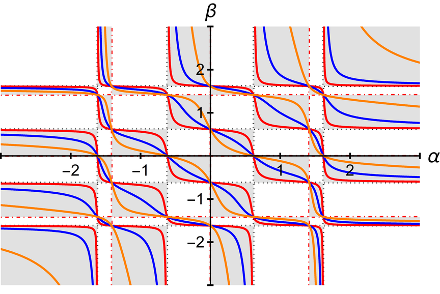
Figure 2: A=B=A1A=B=A_{1} for n=4n=4. Left: Specp⁡(M)\operatorname{Spec}_{p}(M) with κ=0.4\kappa=0.4 (red curves), κ=1\kappa=1 (blue curves) and κ=2\kappa=2 (orange curves). Right: the superimposition of Specp⁡(M)\operatorname{Spec}_{p}(M) for the values of κ\kappa from 0.0010.001 to 1010 with the step-size of 0.10.1.

Note that ΓA1=∅\Gamma_{A_{1}}=\varnothing and the general spectral picture in the (α,β)(\alpha,\beta)-plane including the rectangular mesh can be seen in Figures 2 and 5. We see that the results of the simple Chess Board Theorem hold.

5.2 Example 2

This example illustrates the case when Γ=∅\Gamma=\varnothing. We denote by diag⁡(λ1,…,λn)\operatorname{diag}(\lambda_{1},\dots,\lambda_{n}) a diagonal matrix composed of the entries λ1,…,λn\lambda_{1},\dots,\lambda_{n}. Let A2=diag⁡(−1,1)A_{2}=\operatorname{diag}(-1,1) and B1=diag⁡(1,3)B_{1}=\operatorname{diag}(1,3). Set 𝐳=(1/5,2/5)T\mathbf{z}=\left(1/\sqrt{5},2/\sqrt{5}\right)^{T}. Then ΓA2=ΓB1=∅\Gamma_{A_{2}}=\Gamma_{B_{1}}=\varnothing. Also Spec((A2)⊥,⊥)={−3/5}\operatorname{Spec}((A_{2})_{\bot,\bot})=\left\{-3/5\right\}, Spec⁡((B1)⊥,⊥)={7/5}\operatorname{Spec}((B_{1})_{\bot,\bot})=\left\{7/5\right\}. The spectral picture can be seen in the left of Fig. 3, and we see that the simple Chess Board Theorem (Theorem 2.3) holds.

5.3 Example 3

This example illustrates two cases; the case when Γ≠∅\Gamma\neq\varnothing and Γ~=∅\widetilde{\Gamma}=\varnothing, and also the case when Γ=Γ~≠∅\Gamma=\widetilde{\Gamma}\neq\varnothing. Consider A3=diag⁡(−1,−1)A_{3}=\operatorname{diag}(-1,-1) and B1B_{1}. Set 𝐳=(1,0)T\mathbf{z}=(1,0)^{T}. Then ΓA3={−1}\Gamma_{A_{3}}=\{-1\}, Γ~A3=∅\widetilde{\Gamma}_{A_{3}}=\varnothing, and ΓB1=Γ~B1={3}\Gamma_{B_{1}}=\widetilde{\Gamma}_{B_{1}}=\{3\}. Also Spec⁡((A3)⊥,⊥)={−1}\operatorname{Spec}((A_{3})_{\bot,\bot})=\{-1\}, Spec⁡((B1)⊥,⊥)={3}\operatorname{Spec}((B_{1})_{\bot,\bot})=\{3\}. The spectral picture is shown in the right of Fig. 3. We see that Specp⁡(M)\operatorname{Spec}_{p}(M) has an additional vertical straight line at α=−1\alpha=-1, and there is also a blow-up at α=−1\alpha=-1. This line is included in the mesh since 𝐳\mathbf{z} is orthogonal to one eigenvector but 𝐳⟂̸ΦA3,−1\mathbf{z}\not\perp\Phi_{A_{3},-1}. On the other hand, there is a horizontal straight line passing through β=3\beta=3 which is not included in the mesh since B1B_{1} has simple eigenvalues and 𝐳⟂ΦB1,3\mathbf{z}\perp\Phi_{B_{1},3}.

Refer to caption
Refer to caption
Figure 3: Specp⁡(M)\operatorname{Spec}_{p}(M) for two cases. Left: with A=A2A=A_{2}, B=B1B=B_{1} and κ=2/3\kappa=2/3. Right: with A=A3A=A_{3}, B=B1B=B_{1} and κ=1/2\kappa=1/2.

5.4 Example 4

This example illustrates the case when Γ\Gamma, Γ~≠∅\widetilde{\Gamma}\neq\varnothing and Γ≠Γ~\Gamma\neq\widetilde{\Gamma}. Take

A4=diag⁡(1,1,3,3),B2=(−21001−10000210013).A_{4}=\operatorname{diag}(1,1,3,3),\qquad B_{2}=\begin{pmatrix}-2&1&0&0\\ 1&-1&0&0\\ 0&0&2&1\\ 0&0&1&3\end{pmatrix}. (5.3)

Set 𝐳=(0,0,0,1)T\mathbf{z}=(0,0,0,1)^{T}. Then we have Spec(B2)={−(3±5)/2,(5±5)/2}\operatorname{Spec}(B_{2})=\{-\left(3\pm\sqrt{5}\right)/2,\left(5\pm\sqrt{5}\right)/2\} and ΓA4={1,3}\Gamma_{A_{4}}=\{1,3\}, Γ~A4={1}\widetilde{\Gamma}_{A_{4}}=\{1\} and ΓB2=Γ~B2={−(3±5)/2}\Gamma_{B_{2}}=\widetilde{\Gamma}_{B_{2}}=\{-(3\pm\sqrt{5})/2\}. We also obtain Spec⁡((A4)⊥,⊥)={1,3}\operatorname{Spec}((A_{4})_{\bot,\bot})=\{1,3\}, where the eigenvalue 11 has multiplicity two, and Spec⁡((B2)⊥,⊥)={(−3±5)/2,2}\operatorname{Spec}((B_{2})_{\bot,\bot})=\{\left(-3\pm\sqrt{5}\right)/2,2\}. The spectral picture is shown in the left of Fig. 4. As expected, there are two additional vertical straight lines: at α=1\alpha=1, where is no blow-up and the line is not included in the mesh since 𝐳⟂ΦA4,1\mathbf{z}\perp\Phi_{{A_{4}},1}; and at α=3\alpha=3, where is a blow-up and the line is included in the mesh since 𝐳⟂̸ΦA4,3\mathbf{z}\not\perp\Phi_{{A_{4}},3}. On the other hand, there are two additional horizontal lines at β=−(3±5)/2\beta=-(3\pm\sqrt{5})/2 which are not included in the mesh as 𝐳\mathbf{z} is orthogonal to the corresponding eigenspaces.

5.5 Example 5

This example illustrates the case when Δ≠∅\Delta\neq\varnothing. Consider A5=diag⁡(1,2,2,3)A_{5}=\operatorname{diag}(1,2,2,3), and B2B_{2}. Set 𝐳=(1/2,0,0,1/2)T\mathbf{z}=\left(1/\sqrt{2},0,0,1/\sqrt{2}\right)^{T}. Then ΓA5=Γ~A5={2}\Gamma_{A_{5}}=\widetilde{\Gamma}_{A_{5}}=\{2\} and ΓB2=Γ~B2=∅\Gamma_{B_{2}}=\widetilde{\Gamma}_{B_{2}}=\varnothing. Also Spec⁡((A5)⊥,⊥)={2}\operatorname{Spec}((A_{5})_{\bot,\bot})=\{2\}, where the eigenvalue 22 has multiplicity three, and Spec⁡((B2)⊥,⊥)={(1±13)/2,1/2}\operatorname{Spec}((B_{2})_{\bot,\bot})=\{\left(1\pm\sqrt{13}\right)/2,1/2\}. The spectral picture is shown in the right side of Fig. 4. Since 𝐳⟂ΦA5,2\mathbf{z}\perp\Phi_{A_{5},2}, there is no blow-up at α=2\alpha=2. Nevertheless, this line is included in the mesh as ΔA5={2}\Delta_{A_{5}}=\{2\}, that is, dim(Φ(A5)⊥,⊥,2)>dim(ΦA5,2)\dim\left(\Phi_{(A_{5})_{\bot,\bot},2}\right)>\dim\left(\Phi_{A_{5},2}\right).

Refer to caption
Refer to caption
Figure 4: Specp⁡(M)\operatorname{Spec}_{p}(M) with κ=1\kappa=1 for two cases. Left: with A=A4A=A_{4}, B=B2B=B_{2}. Right: with A=A5A=A_{5}, B=B2B=B_{2}.

6 Relation to a non-self-adjoint problem

We now return to the example studied in [4]. Generally speaking, there are nn complex β⁡(α)∈ℂ\beta(\alpha)\in\mathbb{C} for every α∈Spec⁡(A)∖ℂ\alpha\in\operatorname{Spec}(A)\setminus\mathbb{C}. We therefore limit our attention to pair-eigenvalues subject to the additional restriction

Im⁡(α+β)=0,\mathrm{Im}(\alpha+\beta)=0, (6.1)

which is equivalent to introducing the additional restriction γ∈ℝ\gamma\in\mathbb{R}, see (5.2).

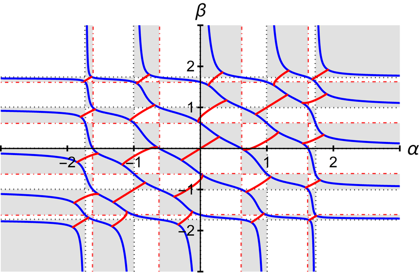
A general spectral picture of this non-self-adjoint problem in the (α,β)(\alpha,\beta)-plane is illustrated in Figure 5. Red curves depict the real parts of non-real pair-eigenvalues Re​β​(Re​α)\mathrm{Re}\ \beta(\mathrm{Re}\ \alpha) such that (6.1) holds, which keeps all (α,β)∈ℝ2(\alpha,\beta)\in\mathbb{R}^{2} in the picture (shown in blue) and also some non-real pair-eigenvalues. It is easily verified that the spectra are symmetric with respect to (α,β)↔(β,α)(\alpha,\beta)\leftrightarrow(\beta,\alpha) and (α,β)↔(−α,−β)(\alpha,\beta)\leftrightarrow(-\alpha,-\beta).

Refer to caption
Figure 5: Specp⁡(M)\operatorname{Spec}_{p}(M) with A=B=A1A=B=A_{1} and C=P1C=P_{1} for n=5n=5.

The real and non-real eigenvalue curves λ⁡(γ)\lambda(\gamma) may collide, with two possible types of collisions: those when two real eigenvalues collide and produce a complex conjugate pair, called Type-A, and those when a pair of complex conjugate eigenvalues collide and become real, called Type-B, see Figure 6 for equivalents in (α,β)(\alpha,\beta)-plane.

Refer to caption
Refer to caption
Refer to caption
Refer to caption
Figure 6: Left: the collisions in the (Re⁡(λ),Im⁡(λ))(\mathrm{Re}(\lambda),\mathrm{Im}(\lambda))-plane. Right: the collisions in the (α,β)(\alpha,\beta)-plane.
Lemma 6.1.

The collisions happen at the points where d​βd​α=−1\frac{d\beta}{d\alpha}=-1.

Proof.

Consider

(A−λ+γCC∗B+λ+γ)​(𝐮𝐯)=𝟎.\displaystyle\begin{pmatrix}A-\lambda+\gamma&C\\ C^{*}&B+\lambda+\gamma\end{pmatrix}\begin{pmatrix}\mathbf{u}\\ \mathbf{v}\end{pmatrix}=\mathbf{0}.

Considering the curves γ⁡(λ)\gamma(\lambda) instead of λ⁡(γ)\lambda(\gamma) and differentiating with respect to λ\lambda we arrive at

(−1+γ′1+γ′)​(𝐮𝐯)=−(A−λ+γCC∗B+λ+γ)​(𝐮′𝐯′),\begin{pmatrix}-1+\gamma^{\prime}&\\ &1+\gamma^{\prime}\end{pmatrix}\begin{pmatrix}\mathbf{u}\\ \mathbf{v}\end{pmatrix}=-\begin{pmatrix}A-\lambda+\gamma&C\\ C^{*}&B+\lambda+\gamma\end{pmatrix}\begin{pmatrix}\mathbf{u^{\prime}}\\ \mathbf{v^{\prime}}\end{pmatrix}, (6.2)

which is solvable if and only if the right hand side of (6.2) is perpendicular to (𝐮𝐯)\begin{pmatrix}\mathbf{u}\\ \mathbf{v}\end{pmatrix}. Therefore multiplying by (𝐮𝐯)\begin{pmatrix}\mathbf{u}\\ \mathbf{v}\end{pmatrix} we obtain

(−1+γ′)​‖𝐮‖2+(1+γ′)​‖𝐯‖2=0\displaystyle(-1+\gamma^{\prime})\|\mathbf{u}\|^{2}+(1+\gamma^{\prime})\|\mathbf{v}\|^{2}=0\quad ⇔γ′(∥𝐮∥2+∥𝐯∥2)=∥𝐮∥2−∥𝐯∥2\displaystyle\Leftrightarrow\quad\gamma^{\prime}(\|\mathbf{u}\|^{2}+\|\mathbf{v}\|^{2})=\|\mathbf{u}\|^{2}-\|\mathbf{v}\|^{2}
⇔γ′=0,\displaystyle\Leftrightarrow\quad\gamma^{\prime}=0,

and since at critical points d​γd​λ=0\frac{d\gamma}{d\lambda}=0, using (5.2) we obtain

d​γd​λ=d​γd​αd​λd​α=−12−12β′12−12β′=0⇔β′=−1.\displaystyle\frac{d\gamma}{d\lambda}=\frac{\frac{d\gamma}{d\alpha}}{\frac{d\lambda}{d\alpha}}=\frac{-\frac{1}{2}-\frac{1}{2}\beta^{{}^{\prime}}}{\frac{1}{2}-\frac{1}{2}\beta^{{}^{\prime}}}=0\quad\Leftrightarrow\quad\beta^{{}^{\prime}}=-1. ∎

Acknowledgments

We are grateful to E. Brian Davies for useful suggestions. The second author acknowledges the financial support by the Ministry of National Education of the Republic of Turkey.

References

  • [1] Atkinson, F. V., 1968. Multiparameter spectral theory. Bull. Amer. Math. Soc. 74(1), 1–27.
  • [2] Atkinson, F. V., 1972. Multiparameters eigenvalue problems. Academic Press, New York-London.
  • [3] Atkinson, F. V., & Mingarelli, A. B., 2011. Multiparameter eigenvalue problems: Sturm–Liouville theory. CRC Press, Boca Raton, FL.
  • [4] Davies, E. B. and Levitin, M., 2014. Spectra of a class of non-self-adjoint matrices. Linear Algebra Appl. 448, 55–84.
  • [5] Sleeman, B. D., 1978. Multiparameter spectral theory in Hilbert space. J. Math. Anal. Appl. 65(3), 511–530.