跳到论文正文
W Papers独立论文阅读器 arXiv:1801.05112 论文正文 计算阅读时间 · 0%
引用这篇论文根据当前论文元数据生成,正式投稿前建议核对。


License: arXiv.org perpetual non-exclusive license
arXiv:1801.05112v4 [cs.IT] 07 Jun 2019

Exact Error and Erasure Exponents for the Asymmetric Broadcast ChannelThanks: D. Cao is with the Southeast University of China (e-mail: dmcao@seu.edu.cn). Thanks: V. Y. F. Tan is with the National University of Singapore (e-mail: vtan@nus.edu.sg). Thanks: D. Cao is supported by the China Scholarship Council (No. 201706090064) and the National Natural Science Foundation of China under Grant No. 61571122. V. Y. F. Tan is supported by a Singapore National Research Foundation (NRF) Fellowship (R-263-000-D02-281).Thanks: This paper was presented in part at the 2018 IEEE International Symposium on Information Theory [1]. Thanks: Copyright (c) 2017 IEEE. Personal use of this material is permitted. However, permission to use this material for any other purposes must be obtained from the IEEE by sending a request to pubs-permissions@ieee.org.

Daming Cao, Student Member, IEEE Affiliation:     Vincent Y. F. Tan, Senior Member, IEEE Affiliation: 
Abstract

Consider the asymmetric broadcast channel with a random superposition codebook, which may be comprised of constant composition or i.i.d. codewords. By applying Forney’s optimal decoder for individual messages and the message pair for the receiver that decodes both messages, exact (ensemble-tight) error and erasure exponents are derived. It is shown that the optimal decoder designed to decode the pair of messages achieves the optimal trade-off between the total and undetected exponents associated with the optimal decoder for the private message. Convex optimization-based procedures to evaluate the exponents efficiently are proposed. Finally, numerical examples are presented to illustrate the results.

Index Terms: 
Broadcast channels, Degraded Message Sets, Erasure decoding, Undetected Error, Error exponents, Superposition coding.

I Introduction

I-A Background and Related Works

The broadcast channel [2] has been extensively studied in multi-user information theory. Although the capacity region is still unknown, some special cases have been solved. One example is the broadcast channel with degraded message sets, also known as the asymmetric broadcast channel (ABC). For this channel, one receiver desires to decode both the private message m1m_{1} and the common message m2m_{2} while the other receiver desires to decode only m2m_{2}. This model can be applied to a plethora of different scenarios; see Section I-D for concrete examples of broadcasting scenarios, taking into account the variation we consider herein.

The capacity region for the ABC was derived by Körner and Marton and is well known [3]. The earliest work on error exponents for the ABC is that by Körner and Sgarro [4], who used a constant composition ensemble for deriving an achievable error exponent. Later, Kaspi and Merhav [5] improved this work by deriving a tighter lower bound for the error exponent by analyzing the ensemble of i.i.d. random codes. Most recently, Averbuch et al. derived the exact random coding error exponents and expurgated exponents for the ensemble of constant composition codes in [6] and [7], respectively.

In this paper, we are interested in decoders with an erasure option. In this setting, the decoders may, instead of declaring that a particular message or set of messages is sent, output an erasure symbol. For the discrete memoryless channel (DMC), Forney [8] found the optimal decoder and derived a lower bound on the total and undetected error exponents using Gallager-style bounding techniques. Csiszár and Körner [9, Thm. 10.11] derived universally attainable erasure and error exponents using a generalization of the maximum mutual information (MMI) decoder. Telatar [10] also analyzed an erasure decoding rule with a general decoding metric. Moulin [11] generalized this family of decoders and proposed a new decoder parameterized by a weighting function. Merhav [12] derived lower bounds to these exponents by using a novel type-class enumerator method. In a breakthrough, Somekh-Baruch and Merhav [13] derived the exact random coding exponents for erasure decoding. Recently, Huleihel et al. [14] showed that the random coding exponent for erasure decoding is not universally achievable and established a simple relation between the total and undetected error exponents. Weinberger and Merhav [15] analyzed a simplified decoder for erasure decoding. Hayashi and Tan [16] derived ensemble-tight moderate deviations and second-order results for erasure decoding over additive DMCs. For the ABC, Tan [17] derived lower bounds on the total and undetected error exponents of an extended version of the universal decoder in Csiszár and Körner [9, Thm. 10.11]. Moreover, Merhav in another landmark work in [18] analyzed a random coding scheme with a binning (superposition coding) structure and showed that a potentially suboptimal bin index decoder achieves the random coding error exponent for decoding only the bin index.

Threshold T = E 1 u E Y u = E 1 t E Y t E 2 u E 2 t T T
Fig. 1: For a fixed rate pair (R1,R2)(R_{1},R_{2}) with varying threshold TT, the figure schematically illustrates E1u,E1t,E2u,E2t,EYuE_{1}^{\mathrm{u}},E_{1}^{\mathrm{t}},E_{2}^{\mathrm{u}},E_{2}^{\mathrm{t}},E_{Y}^{\mathrm{u}}, and EYtE_{Y}^{\mathrm{t}} which are respectively, the undetected exponent for decoding m1m_{1}, the total exponent for decoding m1m_{1}, the undetected exponent for decoding m2m_{2}, the total exponent for decoding m2m_{2}, the undetected exponent for decoding (m1,m2)(m_{1},m_{2}), and the total exponent for decoding (m1,m2)(m_{1},m_{2}). Note that E1u=EYuE_{1}^{\mathrm{u}}=E_{Y}^{\mathrm{u}} and E1t=EYtE_{1}^{\mathrm{t}}=E_{Y}^{\mathrm{t}} so decoding m1m_{1} optimally and (m1,m2)(m_{1},m_{2}) optimally result in the same undetected-total exponent trade-off. Clearly, the same is not true of optimal decoding of m2m_{2} and optimal decoding of (m1,m2)(m_{1},m_{2}).

I-B Main Contributions

In this paper, we consider erasure decoding for the ABC with a superposition codebook structure, in which the distribution of the codewords is either i.i.d. or constant composition. For the decoder that aims to decode both messages, there are six exponents of interest—the total and undetected exponents corresponding to the individual messages m1m_{1} and m2m_{2} and the pair of messages (m1,m2)(m_{1},m_{2}). We derive exact (ensemble-tight) exponents for this problem. The main technical contribution to obtain the exact random coding exponents is a set of tools to handle statistical dependencies between codewords that share the same cloud center. To wit, Lemmas 6 and 7 consists of two technical results that are to establish the equality between the total random coding error exponents pertaining to the first message (i.e., the private message m1m_{1}) and the message pair. This ameliorates the dependency problem, at least on the exponential scale, which is the asymptotic regime of interest.

We show that the minimizations required to evaluate these error exponents can be cast as convex optimization problems, and thus, can be solved efficiently using off-the-shelf convex optimization solvers such as CVX. As such, it is computationally tractable to compare the performance of practical codes to the information-theoretic limits presented here; this guides the design and analysis of future generations of codes. We present numerical examples to illustrate these exponents and the trade-offs involved in the erasure decoding problem for the ABC. We additionally show that the constant composition exponents are, in general, larger than the i.i.d. exponents.

I-C Motivation, Significance, Insights Gleaned, and a Surprise

Our motivation is to find exact (ensemble-tight) erasure and error exponents for the ABC and from the resulting form of the exponents, hope to gain valuable insights into the various trade-offs that are present. In particular, we are interested in whether the optimal decoder for the pair of messages (m1,m2)(m_{1},m_{2}) (at the receiver that is required to decode both messages) performs as well as that for decoding only the private message m1m_{1} or, for that matter, the common message m2m_{2}. Our main observation is that the optimal decoder for (m1,m2)(m_{1},m_{2}) achieves the optimal trade-off between the total and undetected exponents pertaining to m1m_{1}. What are the practical engineering implications and significance of this finding? In a broadcasting setting, the punchline of this paper says that if a communication engineer has the erasure option—e.g., in automatic repeat request/query (ARQ) [8] systems—and desires to only to decipher the private message m1m_{1}, she can essentially obtain the other (common) message m2m_{2} for free using a decoder designed to decode both m1m_{1} and m2m_{2}. By “for free”, we mean that the optimal trade-off in the total and undetected exponents for—i.e., the performance of—decoding m1m_{1} is the same as that for (m1,m2)(m_{1},m_{2}). In view of the packing lemma [19, Lemma 3.1] as applied to broadcast channels [19, Chapters 5 and 8], this observation might seem natural or unsurprising in the rate or capacity sense. However, what we show is much more—indeed, a refined asymptotic result. Our main observation and insight gleaned, which is surprising, implies that on the exponential scale—i.e., in terms of error and erasure exponents—there is no loss in the trade-off whether we choose to decode m1m_{1} or (m1,m2)(m_{1},m_{2}). On the other hand, if the engineer desires to decode only m2m_{2}, she needs to design a dedicated decoder for this task since the optimal trade-off in the total and undetected exponents for the joint decoder is, in general, worse than that of the dedicated one for m2m_{2}. This is illustrated schematically in Figure 1.

I-D Practical, Real-Life Examples

Let us provide practical, real-life examples for which the above theoretical observation is applicable.

Refer to captionNeeds to decode onlylocation of epicenter m 2 Needs to decode bothlocation and actions ( m 1 , m 2 )
Fig. 2: A map of countries affected by the 2004 Indian Ocean tsunami and its epicenter. In Sumatra, both m1m_{1} and m2m_{2} should be broadcasted to the residents. Decoding both is just as reliable, in the sense of total and undetected exponents, as decoding only m1m_{1}. Thus, the main take-home message of this paper is that m2m_{2} comes for free (i.e., E1t=EYtE_{1}^{\mathrm{t}}=E_{Y}^{\mathrm{t}} and E1u=EYuE_{1}^{\mathrm{u}}=E_{Y}^{\mathrm{u}} in Figure 1). In Somalia, though, m2m_{2}, the location of the tsunami’s epicenter is the more salient piece of information and m1m_{1} does not have to be known to the populace since they are unlikely to be required to take any substantial action. The performance of decoding m2m_{2} alone is not the same as decoding (m1,m2)(m_{1},m_{2}) and a dedicated decoder should be designed for the former (i.e., for Somalia). The figure, apart from annotations, is taken from https://en.wikipedia.org/wiki/2004_Indian_Ocean_earthquake_and_tsunami.

On Boxing Day in 2004, the massive Indian Ocean earthquake and tsunami struck. Its epicenter was off the west coast of northern Sumatra, Indonesia. This event resulted in a tremendous loss of lives (roughly a quarter million) and property (roughly worth USD $15 billion) to Indonesia, Sri Lanka, Myanmar, Thailand, the Maldives, and even countries as far as Somalia in East Africa in which damage was present but markedly less severe. See Figure 2. Since then, tsunami warning systems have been set up in Indonesia among other countries. These warning systems (such as DART ® or Deep-ocean Assessment and Reporting of Tsunamis) are used detect tsunamis in advance and to issue warnings to people that might be adversely affected; see [20, 21]. Often, various disparate pieces of information need to be disseminated or broadcast to common folk reliably. For example, those in the direct path of the tsunami may need to know m1m_{1}, the actions they should take to avoid loss of lives (e.g., move to higher ground) and m2m_{2}, the locations in which the tsunami will make landfall and the corresponding severities. For such countries, our result says that if the optimal decoder for (m1,m2)(m_{1},m_{2}) is used, the performance, as defined in Section I-C, is the same as that for decoding only m1m_{1}. Hence, the take-home message is that the residents of Sumatra will, in addition to the actions they need to take, also know the locations the tsunami makes landfall. This can be done without any loss of optimality from the perspective of the trade-off between the error and erasure exponents. For countries that are far away from a major fault line such as Somalia, perhaps the design of a decoder for only m2m_{2} is needed since the presence of the tsunami in Southeast Asia is not likely to require any drastic action from Somalians, so information about m1m_{1} is not needed there. In this case, the Somalian authorities and engineers need to design a dedicated decoder to ensure optimality of decoding m2m_{2} with the erasure option. Note that since tsunami warning systems have the potential to save hundreds of thousands of lives, they have to be ultra reliable. As such, our error and erasure formulation, in which the undetected exponents are designed to be larger than their erasure counterparts (and hence the undetected error probability is exponentially smaller than its erasure counterpart), is of particular relevance in this critical setting. In sum, the findings of our paper have the potential to guide the design and analysis of ultra-reliable infrastructure with varying demands, such as next-generation tsunami warning systems.

Refer to caption X needs Y ( m 1 , m 2 ) needs Z m 2
Fig. 3: A V2V communication network [22] in which receivers have different demands

Another example comes from vehicle-to-vehicle (V2V) communications [22]. In these systems, vehicles form a communication network in which the vehicles themselves are communicating nodes. Through wireless transmissions, they provide each other with crucial information to enhance the safety of all vehicles involved and, in particular, to prevent accidents. For a concrete example, let us consider three vehicles 𝒳\mathcal{X}, 𝒴\mathcal{Y} and 𝒵\mathcal{Z}; see Figure 3. 𝒳\mathcal{X} is in close proximity to 𝒴\mathcal{Y} and thus the two vehicles are likely to collide if no further action is taken. On the other hand, 𝒵\mathcal{Z} is farther away from 𝒳\mathcal{X} than 𝒴\mathcal{Y} is. Hence, in this ultra-reliable setting, 𝒳\mathcal{X} desires to transmit m1m_{1}, the course of actions 𝒴\mathcal{Y} should take to avoid the crash and m2m_{2}, its own location. The good news from our result says that using the optimal decoder, there is no loss in optimality in decoding both messages vis-à-vis only m1m_{1}. Since 𝒵\mathcal{Z} does not need to take any actions at this point in time, it does not need to know m1m_{1} and instead only needs to decode m2m_{2}. The optimal decoder for 𝒵\mathcal{Z} needs to be designed differently from that for m1m_{1} and (m1,m2)(m_{1},m_{2}).

II Problem Formulation

II-A Notation

Throughout this paper, random variables (RVs) will be denoted by upper case letters, their specific values will be denoted by the respective lower case letters, and their alphabets will be denoted by calligraphic letters. A similar convention will apply to random vectors of dimension n∈ℕn\in\mathbb{N} and their realizations. For example, the random vector Xn=(X1,…,Xn)X^{n}=(X_{1},\dots,X_{n}) may take on a certain realization xn=(x1,…,xn)x^{n}=(x_{1},\dots,x_{n}) in 𝒳n\mathcal{X}^{n}, the nn-th order Cartesian power of 𝒳\mathcal{X}, which is the alphabet of each component of this vector.

The distributions associated with random variables will be denoted by the letters PP or QQ, with subscripts being the names of the random variables, e.g., QU​X​YQ_{UXY} stands for a joint distribution of a triple of random variables (U,X,Y)(U,X,Y) on 𝒰×𝒳×𝒴\mathcal{U}\times\mathcal{X}\times\mathcal{Y}, the Cartesian product alphabets of 𝒰\mathcal{U}, 𝒳\mathcal{X} and 𝒴\mathcal{Y}. In accordance with these notations, the joint distribution induced by QYQ_{Y} and QX|YQ_{X|Y} will be denoted by QX​Y:=QY​QX|YQ_{XY}:=Q_{Y}Q_{X|Y}. Information measures induced by the joint distribution QX​YQ_{XY} (or QQ for short) will be subscripted by QQ. For example, IQ​(X,Y)I_{Q}(X;Y) denotes the mutual information of the random variables XX and YY with joint distribution Q=QX​YQ=Q_{XY}.

For a sequence xnx^{n}, let P^xn\hat{P}_{x^{n}} denote its empirical distribution or type. The type class 𝒯PX\mathcal{T}_{P_{X}} of PXP_{X} is the set of all xnx^{n} whose empirical distribution is PXP_{X}. For a given conditional probability distribution PX|UP_{X|U} and sequence unu^{n}, 𝒯PX|U​(un)\mathcal{T}_{P_{X|U}}(u^{n}) denotes the conditional type class of xnx^{n} (PX|UP_{X|U}-shell) given unu^{n}, namely, the set of sequences xnx^{n} whose joint empirical distribution with unu^{n} is given by PX|U​P^unP_{X|U}\hat{P}_{u^{n}}.

The probability of an event ℰ\mathcal{E} will be denoted by Pr⁡{ℰ}\Pr\{\mathcal{E}\}, and the expectation operator with respect to a joint distribution QQ, will be denoted by 𝔼Q​{⋅}\mathbb{E}_{Q}\{\cdot\}. For two positive sequences {an}\{a_{n}\} and {bn}\{b_{n}\}, the notation an≐bna_{n}\doteq b_{n} means that {an}\{a_{n}\} and {bn}\{b_{n}\} are of the same exponential order, i.e., limn→∞1n​ln⁡anbn=0\lim_{n\to\infty}\frac{1}{n}\ln\frac{a_{n}}{b_{n}}=0. Similarly, an≤⋅bna_{n}\stackrel{{\scriptstyle\cdot}}{{\leq}}b_{n} means that lim supn→∞1n​ln⁡anbn≤0\limsup_{n\to\infty}\frac{1}{n}\ln\frac{a_{n}}{b_{n}}\leq 0. The indicator function of an event ℰ\mathcal{E} will be denoted by 𝟙​{ℰ}\mathbbm{1}\{\mathcal{E}\}. The notation |x|+|x|_{+} will stand for max⁡{x,0}\max\{x,0\} and notation [M][M] stands for {1,…,M}\{1,\ldots,M\}. Finally, logarithms and exponents will be understood to be taken to the natural base.

II-B System Model

We consider a discrete memoryless ABC 𝒲:𝒳→𝒴×𝒵\mathcal{W}:\mathcal{X}\to\mathcal{Y}\times\mathcal{Z} with a finite input alphabet 𝒳\mathcal{X}, finite output alphabets 𝒴\mathcal{Y} and 𝒵\mathcal{Z} and a transition probability matrix {W(y,z|x):x∈𝒳,y∈𝒴,z∈𝒵}\{W(y,z|x):x\in\mathcal{X},y\in\mathcal{Y},z\in\mathcal{Z}\}. Let W𝒴:𝒳→𝒴W_{\mathcal{Y}}:\mathcal{X}\to\mathcal{Y} and W𝒵:𝒳→𝒵W_{\mathcal{Z}}:\mathcal{X}\to\mathcal{Z} be respectively the 𝒴\mathcal{Y}- and 𝒵\mathcal{Z}-marginals of WW.

Assume there is a random codebook 𝒞\mathcal{C} with superposition structure for this ABC, where the message pair (m1,m2)(m_{1},m_{2}) is destined for user 𝒴\mathcal{Y} and the common message m2m_{2} is destined for user 𝒵\mathcal{Z}. In this paper, we consider i.i.d. random codes and constant composition random codes.

  • •

    For i.i.d. random codes, fix a distribution PU​X​(u,x)P_{UX}(u,x) and randomly generate M2=en​R2M_{2}=e^{nR_{2}} “cloud centers” {Un​(m2):m2∈ℳ2=[M2]}\{U^{n}(m_{2}):m_{2}\in\mathcal{M}_{2}=[M_{2}]\} according to the distribution

    P⁡(un):=∏i=1nPU​(ui).P(u^{n}):=\prod_{i=1}^{n}P_{U}(u_{i}). (1)

    For each cloud center Un​(m2)U^{n}(m_{2}), randomly generate M1=en​R1M_{1}=e^{nR_{1}} “satellite” codewords {Xn​(m1,m2):m1∈ℳ1=[M1]}\{X^{n}(m_{1},m_{2}):m_{1}\in\mathcal{M}_{1}=[M_{1}]\} according to the conditional probability distribution

    P⁡(xn|un):=∏i=1nPX|U​(xi|ui).\displaystyle P(x^{n}|u^{n}):=\prod_{i=1}^{n}P_{X|U}(x_{i}|u_{i}). (2)
  • •

    For constant composition random codes, we fix a joint type PU​XP_{UX} and randomly and independently generate M2=en​R2M_{2}=e^{nR_{2}} “cloud centers” {Un​(m2):m2∈ℳ2=[M2]}\{U^{n}(m_{2}):m_{2}\in\mathcal{M}_{2}=[M_{2}]\} under the uniform distribution on the type class 𝒯PU\mathcal{T}_{P_{U}}. For each cloud center Un​(m2)U^{n}(m_{2}), randomly and independently generate M1=en​R1M_{1}=e^{nR_{1}} “satellite” codewords {Xn​(m1,m2):m1∈ℳ1=[M1]}\{X^{n}(m_{1},m_{2}):m_{1}\in\mathcal{M}_{1}=[M_{1}]\} under the uniform distribution on the conditional type class 𝒯PX|U​(Un​(m2))\mathcal{T}_{P_{X|U}}(U^{n}(m_{2}))

The two decoders with erasure options are given by g1:𝒴n→(ℳ1∪{e})×(ℳ2∪{e})g_{1}:\mathcal{Y}^{n}\to(\mathcal{M}_{1}\cup\{\mathrm{e}\})\times(\mathcal{M}_{2}\cup\{\mathrm{e}\}) and g2:𝒵n→ℳ2∪{e}g_{2}:\mathcal{Z}^{n}\to\mathcal{M}_{2}\cup\{\mathrm{e}\} where e\mathrm{e} is the erasure symbol.

II-C Definitions of Error Probabilities and Error Exponents

In this paper, there are essentially twelve error probabilities under consideration: the error probabilities of decoding the pair of messages, the error probabilities of decoding the private message m1m_{1} only and the error probabilities of decoding the common message m2m_{2} only. For each of these probabilities, there are the total and undetected error probabilities, and each can be computed at any of the terminals. We focus on six different error probabilities associated to terminal 𝒴\mathcal{Y}. We do not derive the total and undetected error probabilities at terminal 𝒵\mathcal{Z} since the analysis is completely analogous to the analysis of the error and erasure probabilities of the “cloud centers” at terminal 𝒴\mathcal{Y} by replacing W𝒴W_{\mathcal{Y}} with W𝒵W_{\mathcal{Z}}. However, we do compute these exponents numerically in Section V-C (see Figure 9). Define the disjoint decoding regions according to the decoder g1g_{1} as 𝒟m1​m2:={yn:g1​(yn)=(m1,m2)}\mathcal{D}_{m_{1}m_{2}}:=\{y^{n}:g_{1}(y^{n})=(m_{1},m_{2})\}. Moreover, let {𝒟m1:m1∈ℳ1}\{\mathcal{D}_{m_{1}}:m_{1}\in\mathcal{M}_{1}\} and {𝒟m2:m2∈ℳ2}\{\mathcal{D}_{m_{2}}:m_{2}\in\mathcal{M}_{2}\} be the disjoint decoding regions associated to messages m1m_{1} and m2m_{2} respectively. For terminal 𝒴\mathcal{Y}, define for message mj,j=1,2m_{j},j=1,2 and the message pair (m1,m2)(m_{1},m_{2}), the conditional total error and undetected error probabilities as

ejt​(m1,m2):=W𝒴n​(𝒟mjc|xn​(m1,m2))\displaystyle e_{j}^{\mathrm{t}}(m_{1},m_{2}):=W_{\mathcal{Y}}^{n}\big(\mathcal{D}^{c}_{m_{j}}\,\big|\,x^{n}(m_{1},m_{2})\big) (3)
eju​(m1,m2):=W𝒴n​(⋃m^j∈ℳj∖{mj}𝒟m^j|xn​(m1,m2))\displaystyle e_{j}^{\mathrm{u}}(m_{1},m_{2}):=W_{\mathcal{Y}}^{n}\bigg(\bigcup_{\hat{m}_{j}\in\mathcal{M}_{j}\setminus\{m_{j}\}}\mathcal{D}_{\hat{m}_{j}}\,\bigg|\,x^{n}(m_{1},m_{2})\bigg) (4)
eYt​(m1,m2):=W𝒴n​(𝒟m1,m2c|xn​(m1,m2))\displaystyle e_{Y}^{\mathrm{t}}(m_{1},m_{2}):=W_{\mathcal{Y}}^{n}\left(\mathcal{D}^{c}_{m_{1},m_{2}}\,\big|\,x^{n}(m_{1},m_{2})\right) (5)
eYu​(m1,m2):=W𝒴n​(⋃(m^1,m^2)≠(m1,m2)𝒟m^1​m^2|xn​(m1,m2)).\displaystyle e_{Y}^{\mathrm{u}}(m_{1},m_{2}):=W_{\mathcal{Y}}^{n}\bigg(\bigcup_{(\hat{m}_{1},\hat{m}_{2})\neq(m_{1},m_{2})}\mathcal{D}_{\hat{m}_{1}\hat{m}_{2}}\,\bigg|\,x^{n}(m_{1},m_{2})\bigg). (6)

Then we may define the average total and undetected error probabilities at terminal 𝒴\mathcal{Y} as follows:

ejk:=1M1​M2​∑(m1,m2)∈ℳ1×ℳ2ejk​(m1,m2),k∈{t,u}\displaystyle e_{j}^{k}\!:=\!\frac{1}{M_{1}M_{2}}\sum_{(m_{1},m_{2})\in\mathcal{M}_{1}\times\mathcal{M}_{2}}e_{j}^{k}(m_{1},m_{2}),\;\,\,k\in\{\mathrm{t},\mathrm{u}\} (7)
eYk:=1M1​M2​∑(m1,m2)∈ℳ1×ℳ2eYk​(m1,m2),k∈{t,u}.\displaystyle e_{Y}^{k}\!:=\!\frac{1}{M_{1}M_{2}}\sum_{(m_{1},m_{2})\in\mathcal{M}_{1}\times\mathcal{M}_{2}}e_{Y}^{k}(m_{1},m_{2}),\;k\in\{\mathrm{t},\mathrm{u}\}. (8)

Using the Neyman-Pearson theorem, Forney [8] obtained the optimal trade-off between the average total and undetected error probabilities for discrete memoryless channels. By following his idea and using a similar argument, we can show that the optimal trade-off between the average total and undetected error probabilities for the ABC is attained by the following decoding regions11 1 In the following, the threshold TT may take different values depending on whether we are decoding individual messages or the message pair.

𝒟mj∗\displaystyle\mathcal{D}^{*}_{m_{j}} :={yn:Pr⁡(yn|𝒞j​(mj))∑mj′≠mjPr⁡(yn|𝒞j​(mj′))≥en​T},\displaystyle:=\bigg\{y^{n}:\frac{\Pr(y^{n}|\mathcal{C}_{j}(m_{j}))}{\sum_{m^{\prime}_{j}\neq m_{j}}\Pr(y^{n}|\mathcal{C}_{j}(m^{\prime}_{j}))}\geq e^{nT}\bigg\}, (9)
𝒟m1​m2∗\displaystyle\mathcal{D}^{*}_{m_{1}m_{2}} :={yn:W𝒴n​(yn|xn​(m1,m2))∑(m1′,m2′)≠(m1,m2)W𝒴n​(yn|xn​(m1′,m2′))\displaystyle:=\bigg\{y^{n}:\frac{W_{\mathcal{Y}}^{n}(y^{n}|x^{n}(m_{1},m_{2}))}{\sum_{(m^{\prime}_{1},m^{\prime}_{2})\neq(m_{1},m_{2})}W_{\mathcal{Y}}^{n}(y^{n}|x^{n}(m^{\prime}_{1},m^{\prime}_{2}))}
≥en​T},\displaystyle\qquad\qquad\qquad\qquad\qquad\qquad\qquad\geq e^{nT}\bigg\}, (10)

where the distribution of the output yny^{n} conditioned on the subcodebook 𝒞1​(m1)={xn​(m1,m2):m2∈ℳ2}\mathcal{C}_{1}(m_{1})=\{x^{n}(m_{1},m_{2}):m_{2}\in\mathcal{M}_{2}\} is

Pr⁡(yn|𝒞1​(m1)):=1M2​∑m2∈ℳ2W𝒴n​(yn|xn​(m1,m2))\displaystyle\Pr(y^{n}|\mathcal{C}_{1}(m_{1})):=\frac{1}{M_{2}}\sum_{m_{2}\in\mathcal{M}_{2}}W_{\mathcal{Y}}^{n}(y^{n}|x^{n}(m_{1},m_{2})) (11)

and similarly for Pr⁡(yn|𝒞2​(m2))\Pr(y^{n}|\mathcal{C}_{2}(m_{2})).

We would like to find the exact error exponents EjtE^{\mathrm{t}}_{j}, EjuE^{\mathrm{u}}_{j}, EYtE^{\mathrm{t}}_{Y} and EYuE^{\mathrm{u}}_{Y}, j=1,2j=1,2 with the erasure option, i.e., T≥0T\geq 0 (we do not consider the list decoding mode, i.e., T<0T<0, in this paper). These are the exponents associated to the expectation of the error probabilities, where the expectation is taken with respect to the randomness of the codebook 𝒞\mathcal{C} which possess the superposition structure as described in Section II-B. In other words,

E1t​(R1,R2,T):=lim supn→∞[−1n​ln⁡𝔼𝒞​[e1t]],\displaystyle E_{1}^{\mathrm{t}}(R_{1},R_{2},T):=\limsup_{n\to\infty}\left[-\frac{1}{n}\ln\mathbb{E}_{\mathcal{C}}[e^{\mathrm{t}}_{1}]\right], (12)

and similarly for the other exponents E1u,EYt,EYt,E2tE_{1}^{\mathrm{u}},E_{Y}^{\mathrm{t}},E_{Y}^{\mathrm{t}},E_{2}^{\mathrm{t}}, and E2uE_{2}^{\mathrm{u}}. We show, in fact, that the lim sup\limsup in (12) is a limit. These exponents are also called random coding error exponents. If these exponents are known exactly, we say that ensemble-tight results are established.

III Main Results and Discussions

The main result in this paper are stated below in Theorems 1 and 2, establishing exact random coding error exponents for the messages mjm_{j}, j=1,2j=1,2, and the message pair at terminal 𝒴\mathcal{Y}, i.e., the random coding exponents corresponding to the probabilities in (7)–(8).

Before stating our results, we state a few additional definitions. For a given probability distribution Q=QU​X​YQ=Q_{UXY} on 𝒰×𝒳×𝒴\mathcal{U}\times\mathcal{X}\times\mathcal{Y}, rates R1R_{1} and R2R_{2}, and the fixed random coding distribution P=PU​XP=P_{UX}, define

β⁡(Q,R1)\displaystyle\beta(Q,R_{1}) :=D(QX|U∥PX|U|QU)\displaystyle:=D(Q_{X|U}\|P_{X|U}|Q_{U})
+IQ​(X;Y|U)−R1\displaystyle\qquad+I_{Q}(X;Y|U)-R_{1} (13)
γ⁡(Q,R2)\displaystyle\gamma(Q,R_{2}) :=D(QU∥PU)+IQ(U;Y)−R2\displaystyle:=D(Q_{U}\|P_{U})+I_{Q}(U;Y)-R_{2} (14)
Φ⁡(Q,R1,R2)\displaystyle\Phi(Q,R_{1},R_{2}) :=|γ⁡(Q,R2)+|​β​(Q,R1)|+|+\displaystyle:=\big|\gamma(Q,R_{2})+|\beta(Q,R_{1})|_{+}\big|_{+} (15)
Δ⁡(Q,R1,R2)\displaystyle\Delta(Q,R_{1},R_{2}) :=||−γ⁡(Q,R2)|+−β⁡(Q,R1)|+.\displaystyle:=\big||-\gamma(Q,R_{2})|_{+}-\beta(Q,R_{1})\big|_{+}. (16)

III-A Main Results

Theorem 1.

For i.i.d. random codes, the error exponents E1tE_{1}^{\mathrm{t}}, E1uE_{1}^{\mathrm{u}}, EYtE_{Y}^{\mathrm{t}} and EYuE_{Y}^{\mathrm{u}} are given by22 2 In the following analyses and derivations, for ease of notation, we sometimes drop the dependencies of the error exponents (including those in Theorem 2) on the parameters (R1,R2,T)(R_{1},R_{2},T).

E1t​(R1,R2,T)\displaystyle E_{1}^{\mathrm{t}}(R_{1},R_{2},T) =EYt​(R1,R2,T)\displaystyle=E_{Y}^{\mathrm{t}}(R_{1},R_{2},T)
=min⁡{Ψa​(R1,R2,T),Ψb​(R1,T)}\displaystyle=\min\{\Psi_{\mathrm{a}}(R_{1},R_{2},T),\Psi_{\mathrm{b}}(R_{1},T)\} (17)
E1u​(R1,R2,T)\displaystyle E_{1}^{\mathrm{u}}(R_{1},R_{2},T) =EYu​(R1,R2,T)\displaystyle=E_{Y}^{\mathrm{u}}(R_{1},R_{2},T)
=E1t​(R1,R2,T)+T\displaystyle=E_{1}^{\mathrm{t}}(R_{1},R_{2},T)+T (18)

where

Ψa​(R1,R2,T)\displaystyle\Psi_{\mathrm{a}}(R_{1},R_{2},T)
:=minQ^U​X​Y[D(Q^U​X​Y∥PU​X​Y)\displaystyle:=\min_{\hat{Q}_{UXY}}\Big[D(\hat{Q}_{UXY}\|P_{UXY})
+minQU​X|Y∈ℒ1​(Q^X​Y,R1,R2,T)Φ(QU​X|YQ^Y,R1,R2)]\displaystyle\quad+\min_{Q_{UX|Y}\in\mathcal{L}_{1}(\hat{Q}_{XY},R_{1},R_{2},T)}\Phi(Q_{UX|Y}\hat{Q}_{Y},R_{1},R_{2})\Big] (19)
Ψb​(R1,T)\displaystyle\Psi_{\mathrm{b}}(R_{1},T)
:=minQ^U​X​Y[D(Q^U​X​Y∥PU​X​Y)\displaystyle:=\min_{\hat{Q}_{UXY}}\Big[D(\hat{Q}_{UXY}\|P_{UXY})
+minQX|U​Y∈ℒ2​(Q^U​X​Y,R1,T)|β(QX|U​YQ^U​Y,R1)|+]\displaystyle\quad+\min_{Q_{X|UY}\in\mathcal{L}_{2}(\hat{Q}_{UXY},R_{1},T)}|\beta(Q_{X|UY}\hat{Q}_{UY},R_{1})|_{+}\Big] (20)

with PU​X​Y​(u,x,y):=PU​X​(u,x)​W𝒴​(y|x)P_{UXY}(u,x,y):=P_{UX}(u,x)W_{\mathcal{Y}}(y|x) and the sets ℒ1\mathcal{L}_{1} and ℒ2\mathcal{L}_{2} are defined as

ℒ1​(Q^X​Y,R1,R2,T)\displaystyle\mathcal{L}_{1}(\hat{Q}_{XY},R_{1},R_{2},T)
:={QU​X|Y:𝔼Q​ln⁡1W𝒴+𝔼Q^​ln⁡W𝒴−T≤Δ⁡(Q,R1,R2)}\displaystyle\!:=\!\Big\{Q_{UX|Y}\!:\!\mathbb{E}_{Q}\ln\frac{1}{W_{\mathcal{Y}}}\!+\!\mathbb{E}_{\hat{Q}}\ln W_{\mathcal{Y}}\!-\!T\!\leq\!\Delta(Q,R_{1},R_{2})\Big\} (21)
ℒ2​(Q^U​X​Y,R1,T)\displaystyle\mathcal{L}_{2}(\hat{Q}_{UXY},R_{1},T)
:={QX|U​Y:𝔼Q​ln⁡1W𝒴+𝔼Q^​ln⁡W𝒴−T≤|−β⁡(Q,R1)|+},\displaystyle\!:=\!\Big\{Q_{X|UY}\!:\!\mathbb{E}_{Q}\ln\frac{1}{W_{\mathcal{Y}}}\!+\!\mathbb{E}_{\hat{Q}}\ln W_{\mathcal{Y}}\!-\!T\!\leq\!|-\beta(Q,R_{1})\big|_{+}\Big\}, (22)

where QQ in (21) is equal to Q=QU​X|Y​Q^YQ=Q_{UX|Y}\hat{Q}_{Y}, QQ in (22) is equal to Q=QX|U​Y​Q^U​YQ=Q_{X|UY}\hat{Q}_{UY}, and the expectation 𝔼Q^​ln⁡W𝒴\mathbb{E}_{\hat{Q}}\ln W_{\mathcal{Y}} can be explicitly written as ∑u,x,yQ^U​X​Y​(u,x,y)​ln⁡W𝒴​(y|x)\sum_{u,x,y}\hat{Q}_{UXY}(u,x,y)\ln W_{\mathcal{Y}}(y|x).

For constant composition random codes, the corresponding error exponents E1tE_{1}^{\mathrm{t}}, E1uE_{1}^{\mathrm{u}}, EYtE_{Y}^{\mathrm{t}} and EYuE_{Y}^{\mathrm{u}} can be obtained by adding additional constraints to the optimization problems that define the i.i.d. random coding error exponents above. In particular, all joint distributions QU​X​YQ_{UXY} and Q^U​X​Y\hat{Q}_{UXY} that appear in (19)–(22) should satisfy the marginal constraint QU​X=PU​XQ_{UX}=P_{UX}. For example, the corresponding exponent Ψa′\Psi^{\prime}_{\mathrm{a}} for constant composition random codes is given by

Ψ~a​(R1,R2,T)\displaystyle\widetilde{\Psi}_{\mathrm{a}}(R_{1},R_{2},T)
:=minQ^U​X​Y:Q^U​X=PU​X[D(Q^U​X​Y∥PU​X​Y)\displaystyle:=\min_{\hat{Q}_{UXY}:\hat{Q}_{UX}=P_{UX}}\Big[D(\hat{Q}_{UXY}\|P_{UXY})
+minQU​X|Y∈ℒ~1​(Q^X​Y,R1,R2,T)Φ(QU​X|YQ^Y,R1,R2)]\displaystyle\quad\ +\min_{Q_{UX|Y}\in\widetilde{\mathcal{L}}_{1}(\hat{Q}_{XY},R_{1},R_{2},T)}\Phi(Q_{UX|Y}\hat{Q}_{Y},R_{1},R_{2})\Big] (23)

and the set ℒ~1\widetilde{\mathcal{L}}_{1} is defined as

ℒ~1​(Q^X​Y,R1,R2,T)\displaystyle\widetilde{\mathcal{L}}_{1}(\hat{Q}_{XY},R_{1},R_{2},T)
:={QU​X|Y:QU​X=PU​X,\displaystyle:=\Big\{Q_{UX|Y}:Q_{UX}=P_{UX},
𝔼Qln1W𝒴+𝔼Q^lnW𝒴−T≤Δ(Q,R1,R2)}\displaystyle\quad\quad\quad\mathbb{E}_{Q}\ln\frac{1}{W_{\mathcal{Y}}}+\mathbb{E}_{\hat{Q}}\ln W_{\mathcal{Y}}-T\leq\Delta(Q,R_{1},R_{2})\Big\} (24)

where QQ in (24) is equal to Q=QU​X|Y​Q^YQ=Q_{UX|Y}\hat{Q}_{Y} and QU​XQ_{UX} in (24) is the (𝒰×𝒳)(\mathcal{U}\times\mathcal{X})-marginal distribution of QQ.

The proof of Theorem 1 is provided in Section VI. It can be shown that there exists a sequence of (deterministic) codebooks which can simultaneously achieve these following exponents in Theorems 1 and 2 by using Markov’s inequality. (cf. [16, Proof of Theorem 1]).

Theorem 2.

For i.i.d. random codes, the error exponents E2tE_{2}^{\mathrm{t}} and E2uE_{2}^{\mathrm{u}} are given by

E2t​(R1,R2,T)\displaystyle\!\!E_{2}^{\mathrm{t}}(R_{1},R_{2},T) =max⁡{Ψa​(R1,R2,T),Ψc​(R1,R2,T)},\displaystyle\!=\!\max\{\Psi_{\mathrm{a}}(R_{1},R_{2},T),\Psi_{\mathrm{c}}(R_{1},R_{2},T)\}, (25)
E2u​(R1,R2,T)\displaystyle\!\!E_{2}^{\mathrm{u}}(R_{1},R_{2},T) =E2t​(R1,R2,T)+T,\displaystyle\!=\!E_{2}^{\mathrm{t}}(R_{1},R_{2},T)+T, (26)

where

Ψc​(R1,R2,T)\displaystyle\Psi_{\mathrm{c}}(R_{1},R_{2},T)
:=minQ^U​X​Y[D(Q^U​X​Y∥PU​X​Y)\displaystyle:=\min_{\hat{Q}_{UXY}}\Big[D(\hat{Q}_{UXY}\|P_{UXY})
+minQU​X|Y∈ℒ3​(Q^U​X​Y,R1,R2,T)Φ(QU​X|YQ^Y,R1,R2)]\displaystyle\quad+\min_{Q_{UX|Y}\in\mathcal{L}_{3}(\hat{Q}_{UXY},R_{1},R_{2},T)}\Phi(Q_{UX|Y}\hat{Q}_{Y},R_{1},R_{2})\Big] (27)

with

ℒ3​(Q^U​X​Y,R1,R2,T)\displaystyle\mathcal{L}_{3}(\hat{Q}_{UXY},R_{1},R_{2},T)
:={QU​X|Y:𝔼Qln1W𝒴+s0(Q^U​Y,R1)−T\displaystyle:=\Big\{Q_{UX|Y}:\mathbb{E}_{Q}\ln\frac{1}{W_{\mathcal{Y}}}+s_{0}(\hat{Q}_{UY},R_{1})-T
≤Δ(Q,R1,R2)}\displaystyle\qquad\qquad\qquad\qquad\qquad\qquad\quad\leq\Delta(Q,R_{1},R_{2})\Big\} (28)

where QQ in (28) is equal to Q=QU​X|Y​Q^YQ=Q_{UX|Y}\hat{Q}_{Y}, and

s0​(Q^U​Y,R1)\displaystyle s_{0}(\hat{Q}_{UY},R_{1})
:=−minQ~X|U​Y:β⁡(Q~,R1)≤0\displaystyle:=-\min_{\tilde{Q}_{X|UY}:\beta(\tilde{Q},R_{1})\leq 0} [β⁡(Q~,R1)−𝔼Q~​ln⁡W𝒴]\displaystyle\big[\beta(\tilde{Q},R_{1})-\mathbb{E}_{\tilde{Q}}\ln W_{\mathcal{Y}}\big] (29)

and where Q~\tilde{Q} in (29) is equal to Q~=Q~X|U​Y​Q^U​Y\tilde{Q}=\tilde{Q}_{X|UY}\hat{Q}_{UY}.

For constant composition random codes, the error exponents E2tE_{2}^{\mathrm{t}} and E2uE_{2}^{\mathrm{u}} are given by

E2t​(R1,R2,T)\displaystyle\!\!\!\!E_{2}^{\mathrm{t}}(R_{1},R_{2},T) =max⁡{Ψ~a​(R1,R2,T),Ψ~c​(R1,R2,T)},\displaystyle\!=\!\max\big\{\widetilde{\Psi}_{\mathrm{a}}(R_{1},R_{2},T),\widetilde{\Psi}_{\mathrm{c}}(R_{1},R_{2},T)\big\}, (30)
E2u​(R1,R2,T)\displaystyle\!\!\!\!E_{2}^{\mathrm{u}}(R_{1},R_{2},T) =E2t​(R1,R2,T)+T,\displaystyle\!=\!E_{2}^{\mathrm{t}}(R_{1},R_{2},T)+T, (31)

where

Ψ~c​(R1,R2,T)\displaystyle\widetilde{\Psi}_{\mathrm{c}}(R_{1},R_{2},T)
:=minQ^U​X​Y:Q^U​X=PU​X[D(Q^U​X​Y∥PU​X​Y)\displaystyle:=\min_{\hat{Q}_{UXY}:\hat{Q}_{UX}=P_{UX}}\Big[D(\hat{Q}_{UXY}\|P_{UXY})
+minQU​X|Y∈ℒ~3​(Q^U​X​Y,R1,R2,T)Φ(QU​X|YQ^Y,R1,R2)]\displaystyle\quad+\min_{Q_{UX|Y}\in\widetilde{\mathcal{L}}_{3}(\hat{Q}_{UXY},R_{1},R_{2},T)}\Phi(Q_{UX|Y}\hat{Q}_{Y},R_{1},R_{2})\Big] (32)

with

ℒ~3​(Q^U​X​Y,R1,R2,T)\displaystyle\widetilde{\mathcal{L}}_{3}(\hat{Q}_{UXY},R_{1},R_{2},T)
:={QU​X|Y:QU​X=PU​X,\displaystyle:=\Big\{Q_{UX|Y}:Q_{UX}=P_{UX},
𝔼Qln1W𝒴+s~0(Q^U​Y,R1)−T≤Δ(Q,R1,R2)}\displaystyle\quad\mathbb{E}_{Q}\ln\frac{1}{W_{\mathcal{Y}}}+\tilde{s}_{0}(\hat{Q}_{UY},R_{1})-T\leq\Delta(Q,R_{1},R_{2})\Big\} (33)

where QQ in (33) is equal to Q=QU​X|Y​Q^YQ=Q_{UX|Y}\hat{Q}_{Y}, QU​XQ_{UX} in (33) is the (𝒰×𝒳)(\mathcal{U}\times\mathcal{X})-marginal distribution of QQ and

s~0​(Q^U​Y,R1)\displaystyle\tilde{s}_{0}(\hat{Q}_{UY},R_{1})
:=−minQ~X|U​Y:β⁡(Q~,R1)≤0,Q~U​X=PU​X[β(Q~,R1)−𝔼Q~lnW𝒴]\displaystyle:=-\min_{\begin{subarray}{c}\tilde{Q}_{X|UY}:\beta(\tilde{Q},R_{1})\leq 0,\\ \tilde{Q}_{UX}=P_{UX}\end{subarray}}\big[\beta(\tilde{Q},R_{1})-\mathbb{E}_{\tilde{Q}}\ln W_{\mathcal{Y}}\big] (34)

and where Q~\tilde{Q} in (34) is equal to Q~=Q~X|U​Y​Q^U​Y\tilde{Q}=\tilde{Q}_{X|UY}\hat{Q}_{UY} and Q~U​X\tilde{Q}_{UX} in (34) is the (𝒰×𝒳)(\mathcal{U}\times\mathcal{X})-marginal distribution of Q~\tilde{Q}.

The proof of Theorem 2 is provided in Section VII.

III-B Discussion of Main Results

A few remarks on the theorems above are in order.

  • •

    Eqn. (17) in Theorem 1 implies that the optimal decoder for the pair of messages (m1,m2)(m_{1},m_{2}) (i.e., 𝒟m1​m2∗\mathcal{D}_{m_{1}m_{2}}^{*} defined in (10)) achieves the optimal trade-off between the total and undetected error exponents pertaining to the private message m1m_{1}. This observation is non-trivial and not immediately obvious. When 𝒴\mathcal{Y} wishes to decode only the private message m1m_{1}, the optimal decoder for the pair of messages (m1,m2)(m_{1},m_{2}), called the joint decoder, declares the message m^1\hat{m}_{1} of the decoded message pair (m^1,m^2)(\hat{m}_{1},\hat{m}_{2}) is the final output. It is not clear that this decoding strategy is optimal error exponent-wise. The main difference between the error events for these two decoders is that the user 𝒴\mathcal{Y} can decode the correct private message m1m_{1} but the wrong common message m2m_{2}. This is an error event for the joint decoder (but not for the one that focuses only on m1m_{1}). However, Lemma 7 implies that on the exponential scale, the exponents of the two decoders are the same, i.e., there is no loss in optimality in using the joint decoder for decoding only message m1m_{1}.

  • •

    One of our key technical contributions is Lemma 7 (to follow). This lemma allows us to simplify the calculation of the exponents by disentangling the statistical dependencies between “satellite codewords” that share the same cloud center. In particular, when we take into account the fact that the “cloud centers” 𝒞U′\mathcal{C}_{U}^{\prime} (of which there are exponentially many) are random, this lemma allows us to decouple the dependence between two key random variables

    F1=∑m1′∈ℳ1∖{1}∑m2′∈ℳ2∖{1}W𝒴n​(yn|Xn​(m1′,m2′)),F_{1}=\sum_{m^{\prime}_{1}\in\mathcal{M}_{1}\setminus\{1\}}\sum_{m^{\prime}_{2}\in\mathcal{M}_{2}\setminus\{1\}}W_{\mathcal{Y}}^{n}(y^{n}|X^{n}(m^{\prime}_{1},m^{\prime}_{2})), (35)

    and

    F4=∑m2′∈ℳ2∖{1}W𝒴n​(yn|Xn​(1,m2′))F_{4}=\sum_{m^{\prime}_{2}\in\mathcal{M}_{2}\setminus\{1\}}W_{\mathcal{Y}}^{n}(y^{n}|X^{n}(1,m^{\prime}_{2})) (36)

    which are on different sides of a fundamental error probability (see (63) and (95) in the proof of Theorem 1 in Section VI). In contrast, for the analysis of the interference channel in [23] and [24], only an upper bound of the error probability is sought. This upper bound is not necessarily exponentially tight. On the other hand, the use of Lemma 7 incurs no loss in optimality on the exponential scale when appropriately combined with Lemma 6.

  • •

    In an elegant work in [18], Merhav showed that for ordinary channel coding, independent random selection of codewords within a given type class together with suboptimal bin index decoding (which is based on ordinary maximum likelihood decoding), performs as well as optimal bin index decoding in terms of the error exponent achieved. Furthermore, Merhav showed that for constant composition random codes with superposition coding and optimal decoding, the conclusion above no longer holds in general. In this paper, we show that for i.i.d. and constant composition random codes with superposition coding and erasure decoding, the conclusion holds for the case of decoding the “satellite” codewords. That is the (in general) suboptimal decoding of the “satellite” codewords achieves same random coding error exponent as the optimal decoding of the “satellite” codewords (see Theorem 1).

  • •

    In Theorem 1, the total error exponent for the private message m1m_{1} is the minimum of two exponents Ψa\Psi_{\mathrm{a}} and Ψb\Psi_{\mathrm{b}}. The first exponent Ψa\Psi_{\mathrm{a}} intuitively means that the user 𝒴\mathcal{Y} is in a regime where it decodes the pair of messages (m^1,m^2)(\hat{m}_{1},\hat{m}_{2}). Loosely speaking, the second exponent Ψb\Psi_{\mathrm{b}} means that user 𝒴\mathcal{Y} knows the true common message m~2\tilde{m}_{2} (given by a genie), then decodes the “satellite” codeword Xn​(m1,m~2)X^{n}(m_{1},\tilde{m}_{2}). In contrast to the single-user DMC case, now every codeword is generated according to a conditional probability distribution PX|UP_{X|U}. Thus all codewords are conditioned on a particular un​(m~2)u^{n}(\tilde{m}_{2}) sequence rather than being generated according to a marginal distribution PXP_{X}. This is also reflected in the expression of the inner optimization in (20) which is averaged over the random variable UU (see definition of β⁡(⋅)\beta(\cdot) in (13)).

  • •

    In this work, while it seems natural, we do not consider the list decoding mode in which T<0T<0 due to a couple of technical reasons. To ensure that e−n⁡(T+R1)e^{-n(T+R_{1})} in (88) vanishes, Lemma 6 holds on the condition that T>−R1T>-R_{1}, rather than the more general T<0T<0. Furthermore, Lemma 7, which is crucial in removing the dependence between two key random variables F1F_{1} and F4F_{4}, requires that T≥0T\geq 0 due to the derivation of (184). It appears to the authors that relaxations of the conditions on TT in Lemmas 6 and 7 would be rather involved and so we defer the consideration of the list decoding mode to future work.

  • •

    It is clear from the closed-form expressions of the exponents in Theorems 1 and 2 that the constant composition ones are at least as large as their i.i.d. counterparts. In Section V-B, we present a numerical example to show that this inequality can be strict. Furthermore, if the broadcast channel is degraded in favor of 𝒴\mathcal{Y} (i.e., X⊸--Y⊸--ZX\mathrel{\multimap}\joinrel\mathrel{-}\joinrel\mathrel{\mkern-6.0mu}\joinrel\mathrel{-}Y\mathrel{\multimap}\joinrel\mathrel{-}\joinrel\mathrel{\mkern-6.0mu}\joinrel\mathrel{-}Z forms a Markov chain in this order), the error exponents at 𝒵\mathcal{Z} are smaller than that at 𝒴\mathcal{Y}. We also verify this numerically in Section V-C.

  • •

    Finally, for the case in which user 𝒴\mathcal{Y} wishes to decode the common message m2m_{2}, the intuition gleaned from Theorem 2 is that if the decoding is not correct, both events {F1′≥f3e−n​T}\{F^{\prime}_{1}\geq f_{3}e^{-nT}\} and {F1′≥F2e−n​T}\{F^{\prime}_{1}\geq F_{2}e^{-nT}\} should occur (see (140)). This also means that 𝒴\mathcal{Y} can take one of two actions. First, decode the true transmitted codeword Xn​(m1,m2)X^{n}(m_{1},m_{2}) to identify m2m_{2} when the complement of the first event (i.e., {F1′≤f3e−n​T}\{F^{\prime}_{1}\leq f_{3}e^{-nT}\}) occurs; this corresponds to the exponent Ψa\Psi_{\mathrm{a}}. Second it can decode the sub-codebook for the common message 𝒞2′​(m2):={Xn​(m1,m2):m1∈[M1]∖{1}}\mathcal{C}^{\prime}_{2}(m_{2}):=\{X^{n}(m_{1},m_{2}):m_{1}\in[M_{1}]\setminus\{1\}\} to identify m2m_{2} when the second event {F1′≤F2e−n​T}\{F^{\prime}_{1}\leq F_{2}e^{-nT}\} occurs; this corresponds to Ψc\Psi_{\mathrm{c}}. This explains the maximization in the first expression in (25). When R1R_{1} is large, the term Ψc\Psi_{\mathrm{c}} in (27) of Theorem 2 implies that 𝒴\mathcal{Y} is more likely than not to decode the “cloud center” Un​(m2)U^{n}(m_{2}) according to the “test channel” WY|U​(y|u):=∑xW𝒴​(y|x)​PX|U​(x|u)W_{Y|U}(y|u):=\sum_{x}W_{\mathcal{Y}}(y|x)P_{X|U}(x|u). This corresponds to the second decoding strategy, i.e., decoding the entire sub-codebook 𝒞2′​(m2)\mathcal{C}^{\prime}_{2}(m_{2}) indexed by m2m_{2}. Also see Remark 1 to follow.

IV Evaluating the Exponents via Convex Optimization

In this section, we first consider i.i.d. random codes. To evaluate E1tE^{\mathrm{t}}_{1} in Theorem 1, we need to devise an efficient numerical procedure to solve the minimization problems Ψa\Psi_{\mathrm{a}} and Ψb\Psi_{\mathrm{b}}. As will be shown below, these problems can be solved efficiently even though they are not convex.

For the second term Ψb\Psi_{\mathrm{b}} in (20), we can split the feasible region of the inner minimization, i.e., ℒ2​(Q^U​X​Y,R1,T)\mathcal{L}_{2}(\hat{Q}_{UXY},R_{1},T) (see (22)), into two closed sets, namely ℒ21​(Q^U​X​Y):=ℒ2​(Q^U​X​Y,R1,T)∩ℬ1​(Q^U​Y,R1)\mathcal{L}_{21}(\hat{Q}_{UXY}):=\mathcal{L}_{2}(\hat{Q}_{UXY},R_{1},T)\cap\mathcal{B}_{1}(\hat{Q}_{UY},R_{1}) and ℒ22​(Q^U​X​Y):=ℒ2​(Q^U​X​Y,R1,T)∩ℬ2​(Q^U​Y,R1)\mathcal{L}_{22}(\hat{Q}_{UXY}):=\mathcal{L}_{2}(\hat{Q}_{UXY},R_{1},T)\cap\mathcal{B}_{2}(\hat{Q}_{UY},R_{1}), where

ℬ1​(Q^U​Y,R1)\displaystyle\mathcal{B}_{1}(\hat{Q}_{UY},R_{1}) :={QX|U​Y:β⁡(QX|U​Y​Q^U​Y,R1)≥0}\displaystyle:=\{Q_{X|UY}:\beta(Q_{X|UY}\hat{Q}_{UY},R_{1})\geq 0\} (37)
ℬ2​(Q^U​Y,R1)\displaystyle\mathcal{B}_{2}(\hat{Q}_{UY},R_{1}) :={QX|U​Y:β⁡(QX|U​Y​Q^U​Y,R1)≤0}.\displaystyle:=\{Q_{X|UY}:\beta(Q_{X|UY}\hat{Q}_{UY},R_{1})\leq 0\}. (38)

We denote the corresponding minimization problems pertaining to Ψb\Psi_{\mathrm{b}} in (20) (and (22)) in which the function |⋅|+|\cdot|_{+} is inactive or active as Ψb1\Psi_{\mathrm{b}1} and Ψb2\Psi_{\mathrm{b}2}, respectively, i.e.,

Ψb1\displaystyle\Psi_{\mathrm{b}1} :=minQ^U​X​Y[D(Q^U​X​Y∥PU​X​Y)\displaystyle:=\min_{\hat{Q}_{UXY}}\Big[D(\hat{Q}_{UXY}\|P_{UXY})
+minQX|U​Y∈ℒ21​(Q^U​X​Y)β(QX|U​YQ^U​Y,R1)]\displaystyle\qquad+\min_{Q_{X|UY}\in\mathcal{L}_{21}(\hat{Q}_{UXY})}\beta(Q_{X|UY}\hat{Q}_{UY},R_{1})\Big] (39)
Ψb2\displaystyle\Psi_{\mathrm{b}2} :=minQ^U​X​Y:ℒ22​(Q^U​X​Y)≠∅D(Q^U​X​Y∥PU​X​Y),\displaystyle:=\min_{\hat{Q}_{UXY}:\mathcal{L}_{22}(\hat{Q}_{UXY})\neq\emptyset}D(\hat{Q}_{UXY}\|P_{UXY}), (40)

where the sets ℒ21\mathcal{L}_{21} and ℒ22\mathcal{L}_{22} are defined as

ℒ21​(Q^U​X​Y)\displaystyle\mathcal{L}_{21}(\hat{Q}_{UXY})
:={QX|U​Y:𝔼Qln1W𝒴+𝔼Q^lnW𝒴−T≤0,\displaystyle:=\Big\{Q_{X|UY}:\mathbb{E}_{Q}\ln\frac{1}{W_{\mathcal{Y}}}+\mathbb{E}_{\hat{Q}}\ln W_{\mathcal{Y}}-T\leq 0,
β(Q,R1)≥0},\displaystyle\qquad\qquad\qquad\qquad\qquad\qquad\qquad\quad\beta(Q,R_{1})\geq 0\Big\}, (41)
ℒ22​(Q^U​X​Y)\displaystyle\mathcal{L}_{22}(\hat{Q}_{UXY})
:={QX|U​Y:𝔼Qln1W𝒴+𝔼Q^lnW𝒴−T+β(Q,R1)≤0,\displaystyle:=\Big\{Q_{X|UY}:\mathbb{E}_{Q}\ln\frac{1}{W_{\mathcal{Y}}}+\mathbb{E}_{\hat{Q}}\ln W_{\mathcal{Y}}-T+\beta(Q,R_{1})\leq 0,
β(Q,R1)≤0},\displaystyle\qquad\qquad\qquad\qquad\qquad\qquad\qquad\quad\beta(Q,R_{1})\leq 0\Big\}, (42)

and where QQ in (41) and (42) is equal to Q=QX|U​Y​Q^U​YQ=Q_{X|UY}\hat{Q}_{UY}. We thus have Ψb=min⁡{Ψb1,Ψb2}\Psi_{\mathrm{b}}=\min\{\Psi_{\mathrm{b}1},\Psi_{\mathrm{b}2}\}.

As the minimization problem Ψb2\Psi_{\mathrm{b}2} is convex, it can be solved efficiently. However Ψb1\Psi_{\mathrm{b}1} is non-convex due to the non-convex constraint β⁡(QX|U​Y​Q^U​Y)≥0\beta(Q_{X|UY}\hat{Q}_{UY})\geq 0 in the inner optimization.33 3 In this section, we drop the dependences of β⁡(⋅)\beta(\cdot) and γ⁡(⋅)\gamma(\cdot) on the rates R1R_{1} and R2R_{2} For the inner optimization, if we remove this constraint in ℒ21\mathcal{L}_{21}, the modified problem is

Ψb1′\displaystyle\Psi^{\prime}_{\mathrm{b}1} :=minQ^U​X​Y[D(Q^U​X​Y∥PU​X​Y)\displaystyle:=\min_{\hat{Q}_{UXY}}\Big[D(\hat{Q}_{UXY}\|P_{UXY})
+minQX|U​Y∈ℒ21′​(Q^U​X​Y)β(QX|U​YQ^U​Y)],\displaystyle\qquad+\min_{Q_{X|UY}\in\mathcal{L}^{\prime}_{21}(\hat{Q}_{UXY})}\beta(Q_{X|UY}\hat{Q}_{UY})\Big], (43)

where

ℒ21′​(Q^U​X​Y)\displaystyle\mathcal{L}^{\prime}_{21}(\hat{Q}_{UXY})
:={QX|U​Y:𝔼Q​ln⁡1W𝒴+𝔼Q^​ln⁡W𝒴−T≤0},\displaystyle:=\Big\{Q_{X|UY}:\mathbb{E}_{Q}\ln\frac{1}{W_{\mathcal{Y}}}+\mathbb{E}_{\hat{Q}}\ln W_{\mathcal{Y}}-T\leq 0\Big\}, (44)

is convex and can be solved efficiently. Furthermore, we have the following proposition.

Proposition 3.

For the optimization problem Ψb1\Psi_{\mathrm{b}1}, if the optimal solution to the inner optimization of the modified problem Ψb1′\Psi^{\prime}_{\mathrm{b}1} is not feasible for the original problem Ψb1\Psi_{\mathrm{b}1}, i.e., β⁡(QX|U​Y​Q^U​Y)<0\beta(Q_{X|UY}\hat{Q}_{UY})<0, then there exists an optimal solution to the original inner optimization problem that satisfies β⁡(QX|U​Y​Q^U​Y)=0\beta(Q_{X|UY}\hat{Q}_{UY})=0. Moreover, in this case, the optimal value of Ψb\Psi_{\mathrm{b}} is equal that for Ψb2\Psi_{\mathrm{b}2} (i.e., Ψb2\Psi_{\mathrm{b}2} is active in the minimum that defines Ψb\Psi_{\mathrm{b}}).

Proof:

See Appendix A. ∎In summary, we can solve the non-convex optimization problem Ψb\Psi_{\mathrm{b}} by solving two convex problems Ψb2\Psi_{\mathrm{b}2} and Ψb1′\Psi^{\prime}_{\mathrm{b}1}, i.e.,

Ψb=min⁡{(Ψb1′)+,Ψb2},\displaystyle\Psi_{\mathrm{b}}=\min\{(\Psi^{\prime}_{\mathrm{b}1})^{+},\Psi_{\mathrm{b}2}\}, (45)

where the superscript “++” of (Ψb1′)+(\Psi^{\prime}_{\mathrm{b}1})^{+} means the value of (Ψb1′)+(\Psi^{\prime}_{\mathrm{b}1})^{+} is active in the minimization if the optimal solution (Q^∗,Q∗)(\hat{Q}^{*},Q^{*}) is also feasible for the original optimization Ψb1\Psi_{\mathrm{b}1}, i.e., β⁡(QX|U​Y∗​Q^U​Y∗)≥0\beta(Q^{*}_{X|UY}\hat{Q}^{*}_{UY})\geq 0. In other words,

Ψb={min⁡{Ψb1′,Ψb2}β⁡(QX|U​Y∗​Q^U​Y∗)≥0Ψb2else.\displaystyle\Psi_{\mathrm{b}}=\left\{\begin{aligned} &\min\{\Psi^{\prime}_{\mathrm{b}1},\Psi_{\mathrm{b}2}\}\quad&&\beta(Q^{*}_{X|UY}\hat{Q}^{*}_{UY})\geq 0\\ &\Psi_{\mathrm{b}2}&&\text{else}\end{aligned}\right.. (46)

Consequently, Ψb\Psi_{\mathrm{b}} can be solved efficiently.

For Ψa\Psi_{\mathrm{a}} in (19), let

Ω⁡(QU​X|Y​Q^Y)\displaystyle\Omega(Q_{UX|Y}\hat{Q}_{Y})
:=𝔼QU​X|Y​Q^Y​ln⁡1W𝒴+𝔼Q^​ln⁡W𝒴−T,\displaystyle:=\mathbb{E}_{Q_{UX|Y}\hat{Q}_{Y}}\ln\frac{1}{W_{\mathcal{Y}}}+\mathbb{E}_{\hat{Q}}\ln W_{\mathcal{Y}}-T, (47)

then similarly, we can partition the feasible region of the inner minimization into four parts and denote the corresponding inner optimization problems as follows:

  1. 1.

    If γ⁡(Q)≥0\gamma(Q)\geq 0 and β⁡(Q)≥0\beta(Q)\geq 0, then

    Φa1∗:=minQ⁡γ⁡(Q)+β⁡(Q),such thatΩ⁡(Q)≤0.\displaystyle\Phi_{\mathrm{a}1}^{*}:=\min_{Q}\gamma(Q)+\beta(Q),\ \ \mbox{such that}\ \ \Omega(Q)\leq 0. (48)
  2. 2.

    If γ⁡(Q)≥0\gamma(Q)\geq 0 and β⁡(Q)≤0\beta(Q)\leq 0, then

    Φa2∗:=minQ⁡γ⁡(Q),such thatΩ⁡(Q)+β⁡(Q)≤0.\displaystyle\Phi_{\mathrm{a}2}^{*}:=\min_{Q}\gamma(Q),\ \ \mbox{such that}\ \ \Omega(Q)+\beta(Q)\leq 0. (49)
  3. 3.

    If γ⁡(Q)≤0\gamma(Q)\leq 0 and γ⁡(Q)+β⁡(Q)≥0\gamma(Q)+\beta(Q)\geq 0, then

    Φa3∗:=minQ⁡γ⁡(Q)+β⁡(Q),such thatΩ⁡(Q)≤0.\displaystyle\Phi_{\mathrm{a}3}^{*}:=\min_{Q}\gamma(Q)+\beta(Q),\ \ \mbox{such that}\ \ \Omega(Q)\leq 0. (50)
  4. 4.

    If γ⁡(Q)≤0\gamma(Q)\leq 0 and γ⁡(Q)+β⁡(Q)≤0\gamma(Q)+\beta(Q)\leq 0, then

    Φa4∗:=0such thatΩ⁡(Q)+γ⁡(Q)+β⁡(Q)≤0.\displaystyle\Phi_{\mathrm{a}4}^{*}:=0\ \ \mbox{such that}\ \ \Omega(Q)+\gamma(Q)+\beta(Q)\leq 0. (51)

where QQ in the above definitions is equal to Q=QU​X|Y​Q^YQ=Q_{UX|Y}\hat{Q}_{Y} (compare the above to the definition of the optimization problem Ψa\Psi_{\mathrm{a}} in (19)). Thus we have,

Ψa=minQ^U​X​Y[D(Q^U​X​Y∥PU​X​Y)+mini∈[4]{Φa​i∗(Q^X​Y)}].\displaystyle\Psi_{\mathrm{a}}=\min_{\hat{Q}_{UXY}}\big[D(\hat{Q}_{UXY}\|P_{UXY})+\min_{i\in[4]}\{\Phi^{*}_{\mathrm{a}i}({\hat{Q}_{XY}})\}\big]. (52)

We can rewrite the objective functions of Φa1∗\Phi_{\mathrm{a}1}^{*} and Φa3∗\Phi_{\mathrm{a}3}^{*} as follows

minQU​X|Y⁡γ⁡(QU​X|Y​Q^Y)+β⁡(QU​X|Y​Q^Y)\displaystyle\min_{Q_{UX|Y}}\gamma(Q_{UX|Y}\hat{Q}_{Y})+\beta(Q_{UX|Y}\hat{Q}_{Y})
=minQU|Y⁡[γ⁡(QU|Y​Q^Y)+minQX|U​Y⁡β⁡(QX|U​Y​QU|Y​Q^Y)]\displaystyle=\min_{Q_{U|Y}}[\gamma(Q_{U|Y}\hat{Q}_{Y})+\min_{Q_{X|UY}}\beta(Q_{X|UY}Q_{U|Y}\hat{Q}_{Y})] (53)

where the notation γ⁡(QU|Y​Q^Y)\gamma(Q_{U|Y}\hat{Q}_{Y}) is consistent due to the fact that the function γ⁡(Q,R2)\gamma(Q,R_{2}) (see (14)) only depends on the marginal distribution QU​YQ_{UY}. Therefore, by using a similar argument as that for Ψb1\Psi_{\mathrm{b}1} above, we can remove the non-convex constraint β⁡(Q)≥0\beta(Q)\geq 0 in Φa1∗\Phi_{\mathrm{a}1}^{*} due to Φa2∗\Phi_{\mathrm{a}2}^{*}. We can also remove the non-convex constraint γ⁡(Q)+β⁡(Q)≥0\gamma(Q)+\beta(Q)\geq 0 in Φa3∗\Phi_{\mathrm{a}3}^{*} due to Φa4∗\Phi_{\mathrm{a}4}^{*}. Denote these two modified optimizations as Φa1′\Phi_{\mathrm{a}1}^{\prime} and Φa3′\Phi_{\mathrm{a}3}^{\prime}, respectively. We can merge these two modified optimizations Φa1′\Phi_{\mathrm{a}1}^{\prime} and Φa3′\Phi_{\mathrm{a}3}^{\prime} into a new convex optimization problem Φa5∗\Phi_{\mathrm{a}5}^{*} i.e.,

Φa5∗:=min⁡γ⁡(Q)+β⁡(Q)such thatΩ⁡(Q)≤0.\displaystyle\Phi_{\mathrm{a}5}^{*}:=\min\gamma(Q)+\beta(Q)\quad\mbox{such that}\quad\Omega(Q)\leq 0. (54)

We now state and prove a proposition that simplifies the calculation of (52).

Proposition 4.

For the inner minimization problem in (52), i.e., mini∈[4]⁡{Φa​i∗​(Q^X​Y)}\min_{i\in[4]}\{\Phi^{*}_{\mathrm{a}i}(\hat{Q}_{XY})\}, without loss of optimality, we can replace Φa1∗\Phi_{\mathrm{a}1}^{*} and Φa3∗\Phi_{\mathrm{a}3}^{*} with the new convex optimization problem Φa5∗\Phi_{\mathrm{a}5}^{*}.

Proof:

See Appendix B. ∎For the second term Ψa2\Psi_{\mathrm{a}2}, we can also remove the non-convex constraint γ⁡(Q)≥0\gamma(Q)\geq 0 in Φa2∗\Phi_{\mathrm{a}2}^{*} due to Φa4∗\Phi_{\mathrm{a}4}^{*}. Therefore, we can solve the minimization problem Ψa\Psi_{\mathrm{a}} in (19) efficiently, as the remaining case Φa4∗\Phi_{\mathrm{a}4}^{*} is a convex minimization problem.

Similarly to the above, we can also efficiently calculate E2tE_{2}^{\mathrm{t}} in Theorem 2 as s0​(Q^,R1)s_{0}(\hat{Q},R_{1}) is a convex minimization problem.

Finally, for constant composition random codes, since the additional marginal constraints are linear, the transformed optimization problems remain convex and can be solved efficiently as we show in Section V-B.

V Numerical Evaluations

In this section, we present numerical examples to illustrate the following.

  • •

    The behavior of the i.i.d. exponents in Theorems 1 and 2;

  • •

    The comparison between the constant composition and the i.i.d. error exponents in Theorem 1;

  • •

    The comparison between the i.i.d. error exponents for message m2m_{2} at terminals 𝒴\mathcal{Y} and 𝒵\mathcal{Z}.

We consider binary symmetric channels (BSCs): Y=X⊕V1Y=X\oplus V_{1} and Z=X⊕V2Z=X\oplus V_{2}, where X,Y,V1,V2∈{0,1}X,Y,V_{1},V_{2}\in\{0,1\}, V1∼Bern​(p1)V_{1}\sim\text{Bern}(p_{1}) and V2∼Bern​(p2)V_{2}\sim\text{Bern}(p_{2}). Let UU be binary as well and U∼Bern​(0.5)U\sim\text{Bern}(0.5). Also, let X=U⊕V3X=U\oplus V_{3}, where V3∈{0,1}V_{3}\in\{0,1\} and V3∼Bern​(q)V_{3}\sim\text{Bern}(q). In this example, we fix p1=0.2p_{1}=0.2, p2=0.25p_{2}=0.25 and q=0.1q=0.1, and all the rates are in nats.

All the Matlab® code to reproduce Figures 4–9 can be found at https://www.ece.nus.edu.sg/stfpage/vtan/isit18.zip.
Refer to caption

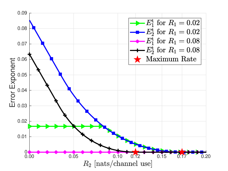
Fig. 4: Total error exponents E1tE_{1}^{\mathrm{t}} and E2tE_{2}^{\mathrm{t}} as a function of R2R_{2} for two different values of R1R_{1} and where the threshold T=0T=0.

Refer to caption

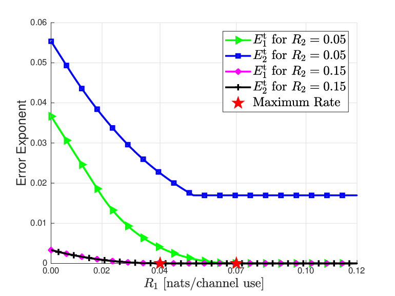
Fig. 5: Total error exponents E1tE_{1}^{\mathrm{t}} and E2tE_{2}^{\mathrm{t}} as a function of R1R_{1} for two different values of R2R_{2} and where the threshold T=0T=0.

Refer to caption

Fig. 6: Total error exponent E1tE^{\mathrm{t}}_{1} and undetected error exponent E1uE^{\mathrm{u}}_{1} for message m1m_{1} as a function of TT for two different pairs of (R1,R2)(R_{1},R_{2}).

Refer to caption

Fig. 7: Total error exponent E2tE^{\mathrm{t}}_{2} and undetected error exponent E2uE^{\mathrm{u}}_{2} for message m2m_{2} as a function of TT for two different pairs of (R1,R2)(R_{1},R_{2}).

V-A Behavior of i.i.d. Exponents

Firstly, we consider the i.i.d. case in which T=0T=0. We obtain a three-dimensional exponent-rate region (Ejt,R1,R2)(E^{\mathrm{t}}_{j},R_{1},R_{2}) for decoding (m1,m2)(m_{1},m_{2}). To obtain a two-dimensional plot, we consider projections: Fix one rate and vary the other rate and plot the error exponent EjtE^{\mathrm{t}}_{j}, j=1,2j=1,2. Figure 4 shows one projection for R1=0.02R_{1}=0.02 and R1=0.08R_{1}=0.08 nats/channel use. For message m1m_{1}, the range of R2R_{2} for which E1t>0E^{\mathrm{t}}_{1}>0 (i.e., R2<0.17R_{2}<0.17 for R1=0.02R_{1}=0.02 and R2=0R_{2}=0 for R1=0.08R_{1}=0.08) coincides with that for the set of achievable rate pairs (R1,R2)(R_{1},R_{2}) corresponding to our choice of input distribution PU​XP_{UX} for decoding only message m1m_{1}, namely44 4 The rate region in (55) and (56) can be obtained by applying the packing lemma in [19, Lemma 3]. Also see [19, Sec. 5.3.1] for a similar analysis of the superposition coding inner bound.

{R1≤I(X;Y|U)=0.07}\displaystyle\{R_{1}\leq I(X;Y|U)=0.07\}
⋂{R1+R2≤I(X;Y)=0.19}.\displaystyle\qquad\,\bigcap\,\{R_{1}+R_{2}\leq I(X;Y)=0.19\}. (55)

Moreover, we see that E1tE^{\mathrm{t}}_{1} for a fixed R1R_{1} is horizontal for R2R_{2} below a critical value and curved for R2R_{2} above this value. For message m1m_{1}, the range of R2R_{2} for which E2t>0E^{\mathrm{t}}_{2}>0 (i.e., R2<0.17R_{2}<0.17 for R1=0.02R_{1}=0.02 and R2<0.12R_{2}<0.12 for R1=0.08R_{1}=0.08) coincides that for the set of achievable rate pairs (R1,R2)(R_{1},R_{2}) corresponding to our choice of input distribution PU​XP_{UX} for decoding only m2m_{2}, i.e.,

{R2≤I(U;Y)=0.12}\displaystyle\{R_{2}\leq I(U;Y)=0.12\}
⋃{R1+R2≤I(X;Y)=0.19}.\displaystyle\qquad\,\bigcup\,\{R_{1}+R_{2}\leq I(X;Y)=0.19\}. (56)

Figure 5 shows the other projection for R2=0.05R_{2}=0.05 and R2=0.15R_{2}=0.15 nats/channel use. It also can be checked that the range of R1R_{1} for both messages (m1,m2)(m_{1},m_{2}) coincides with (55). When R2=0.05≤I⁡(U,Y)R_{2}=0.05\leq I(U;Y), we see the curve of E2tE^{\mathrm{t}}_{2} rapidly decreases for R1R_{1} below a critical value and remains horizontal for R1R_{1} above the critical value. This is because when R2=0.05≤I⁡(U,Y)R_{2}=0.05\leq I(U;Y), the rate pair (R1,R2)(R_{1},R_{2}) is always achievable, i.e., (R1,R2)(R_{1},R_{2}) belongs to the region defined in (56). When R2=0.15≥I⁡(U,Y)R_{2}=0.15\geq I(U;Y), we observe that the two error exponents E1tE^{\mathrm{t}}_{1} and E2tE^{\mathrm{t}}_{2} are equal.

Figures 6 and 7 illustrate the optimal trade-off between the i.i.d. total error exponent and the i.i.d. undetected error exponent as function of TT for two different pairs of (R1,R2)(R_{1},R_{2}). We observe that for both messages, the total error exponent decreases and the undetected error exponent increases when the threshold TT increases. We also observe that the smallest threshold TT for which the total error exponent is zero depends on the rate pair (R1,R2)(R_{1},R_{2}) and decreases as either rate increases.

Refer to caption

Fig. 8: Constant composition and i.i.d. total error exponents E~1t\tilde{E}^{\mathrm{t}}_{1} and E1tE^{\mathrm{t}}_{1} for message m1m_{1} as a function of TT for two different pairs of (R1,R2)(R_{1},R_{2}).

V-B Gain of Constant Composition Exponents over i.i.d. Ones

We now demonstrate the gain of the constant composition exponents over the i.i.d. ones in Theorem 1. Denote the constant composition and i.i.d. total error exponents for m1m_{1} as E~1t\tilde{E}^{\mathrm{t}}_{1} and E1tE^{\mathrm{t}}_{1} respectively. For the example of BSCs described at the start of this section, Figure 8 displays these exponents as functions of TT for two different pairs of (R1,R2)(R_{1},R_{2}). We observe that the constant composition exponents are strictly larger than their i.i.d. counterparts.

V-C Comparison of i.i.d. Exponents at Two Terminals

Finally, we consider the relationship between the exponents at the two terminals. We denote the i.i.d. total and undetected error exponent for m2m_{2} at terminal 𝒵\mathcal{Z} as E2,𝒵tE^{\mathrm{t}}_{2,\mathcal{Z}} and E2,𝒵uE^{\mathrm{u}}_{2,\mathcal{Z}} respectively. Figure 9 compares the optimal trade-off between these exponents as functions of TT for terminals 𝒴\mathcal{Y} and 𝒵\mathcal{Z}. We observe that similar to the standard decoding, if the channel quality is worse, this leads to a smaller exponent for the decoding with erasure option (and vice versa).

Refer to caption

Fig. 9: Total and undetected error exponents E2uE^{\mathrm{u}}_{2} and E2tE^{\mathrm{t}}_{2} at terminal 𝒴\mathcal{Y} and E2,𝒵uE^{\mathrm{u}}_{2,\mathcal{Z}} and E2,𝒵tE^{\mathrm{t}}_{2,\mathcal{Z}} at terminal 𝒵\mathcal{Z} for message m2m_{2} as a function of TT for a given rate pair (R1,R2)=(0.01,0.01)(R_{1},R_{2})=(0.01,0.01).

VI Proof of Theorem 1

Proof:

Firstly, we consider i.i.d. random codes. At the end of the proof, we describe how to extend the analysis to constant composition codes. Assume, without loss of generality, that the true transmitted message pair is (m1,m2)=(1,1)(m_{1},m_{2})=(1,1). Denote the random sub-codebook {Un​(m2′):m2′∈ℳ2∖{1}}\{U^{n}(m^{\prime}_{2}):m^{\prime}_{2}\in\mathcal{M}_{2}\setminus\{1\}\} as 𝒞U′\mathcal{C}^{\prime}_{U}, and the (total) error event ℰ1\mathcal{E}_{1} as

ℰ1:={∑m1′≠1Pr(Yn|𝒞1(m1′))>Pr(Yn|𝒞1(1))e−n​T}.\displaystyle\mathcal{E}_{1}\!:=\!\bigg\{\sum_{m^{\prime}_{1}\neq 1}\Pr(Y^{n}|\mathcal{C}_{1}(m^{\prime}_{1}))\!>\!\Pr(Y^{n}|\mathcal{C}_{1}(1))e^{-nT}\bigg\}. (57)

Given the optimal decoding region 𝒟m1∗\mathcal{D}_{m_{1}}^{*} in (9), by using the law of total probability, the average total error probability for message m1=1m_{1}=1 is

𝔼𝒞​[e1t​(1,1)]=𝔼(Un​(1),Xn​(1,1),Yn)\displaystyle\mathbb{E}_{\mathcal{C}}[e_{1}^{\mathrm{t}}(1,1)]=\mathbb{E}_{(U^{n}(1),X^{n}(1,1),Y^{n})}
[𝔼𝒞U′[Pr{ℰ1|(Un(1),Xn(1,1),Yn),𝒞U′}]],\displaystyle\qquad\qquad\Big[\mathbb{E}_{\mathcal{C}^{\prime}_{U}}\big[\Pr\{\mathcal{E}_{1}|(U^{n}(1),X^{n}(1,1),Y^{n}),\mathcal{C}^{\prime}_{U}\}\big]\Big], (58)

Next, we calculate the error probability given (Un​(1),Xn​(1,1),Yn)=(un,xn,yn)(U^{n}(1),X^{n}(1,1),Y^{n})=(u^{n},x^{n},y^{n}) with joint type Q^U​X​Y\hat{Q}_{UXY} and the sub-codebook 𝒞U′=cU′\mathcal{C}^{\prime}_{U}=c^{\prime}_{U}. For brevity, define the quantities

F1\displaystyle F_{1} :=∑m1′∈ℳ1∖{1}∑m2′∈ℳ2∖{1}W𝒴n​(yn|Xn​(m1′,m2′))\displaystyle:=\sum_{m^{\prime}_{1}\in\mathcal{M}_{1}\setminus\{1\}}\sum_{m^{\prime}_{2}\in\mathcal{M}_{2}\setminus\{1\}}W_{\mathcal{Y}}^{n}(y^{n}|X^{n}(m^{\prime}_{1},m^{\prime}_{2})) (59)
F2\displaystyle F_{2} :=∑m1′∈ℳ1∖{1}W𝒴n​(yn|Xn​(m1′,1))\displaystyle:=\sum_{m^{\prime}_{1}\in\mathcal{M}_{1}\setminus\{1\}}W_{\mathcal{Y}}^{n}(y^{n}|X^{n}(m^{\prime}_{1},1)) (60)
f3\displaystyle f_{3} :=W𝒴n​(yn|xn)\displaystyle:=W_{\mathcal{Y}}^{n}(y^{n}|x^{n}) (61)
F4\displaystyle F_{4} :=∑m2′∈ℳ2∖{1}W𝒴n​(yn|Xn​(1,m2′)).\displaystyle:=\sum_{m^{\prime}_{2}\in\mathcal{M}_{2}\setminus\{1\}}W_{\mathcal{Y}}^{n}(y^{n}|X^{n}(1,m^{\prime}_{2})). (62)

Note that f3f_{3} is a deterministic quantity given (Xn​(1,1),Yn)=(xn,yn)(X^{n}(1,1),Y^{n})=(x^{n},y^{n}) while the others are random. These definitions allow us to express Pr⁡{ℰ1}\Pr\{\mathcal{E}_{1}\} compactly as55 5 In the following analysis, for ease of notation, we drop the conditioning events {Un(1),Xn(1,1),Yn)=(un,xn,yn)}\{U^{n}(1),X^{n}(1,1),Y^{n})=(u^{n},x^{n},y^{n})\} and {𝒞U′=cU′}\{\mathcal{C}^{\prime}_{U}=c^{\prime}_{U}\} when there is no possibility of confusion.

Pr{ℰ1}=Pr{F1+F2>(f3+F4)⋅e−n​T}.\displaystyle\Pr\{\mathcal{E}_{1}\}=\Pr\left\{F_{1}+F_{2}>(f_{3}+F_{4})\cdot e^{-nT}\right\}. (63)

Let QU|YQ_{U|Y}, QU​X|YQ_{UX|Y} and QX|U​YQ_{X|UY} be conditional types such that QU|Y​Q^YQ_{U|Y}\hat{Q}_{Y}, QU​X|Y​Q^YQ_{UX|Y}\hat{Q}_{Y} and QX|U​Y​Q^U​YQ_{X|UY}\hat{Q}_{UY} are joint types defined on 𝒰×𝒴\mathcal{U}\times\mathcal{Y}, 𝒰×𝒳×𝒴\mathcal{U}\times\mathcal{X}\times\mathcal{Y} and 𝒰×𝒳×𝒴\mathcal{U}\times\mathcal{X}\times\mathcal{Y}, respectively. Define the following quantities

Λ⁡(QU​Y,𝒞U′)\displaystyle\Lambda(Q_{UY},\mathcal{C}^{\prime}_{U}) :=|{Un(m2):m2∈ℳ2∖{1},\displaystyle:=\big|\big\{U^{n}(m_{2}):m_{2}\in\mathcal{M}_{2}\setminus\{1\},
(Un(m2),yn)∈𝒯QU​Y}|,\displaystyle\qquad(U^{n}(m_{2}),y^{n})\in\mathcal{T}_{Q_{UY}}\big\}\big|, (64)
Nm1​(QU​X​Y)\displaystyle N_{m_{1}}(Q_{UXY}) :=|{Xn(m1,m2):m2∈ℳ2∖{1},\displaystyle:=\big|\big\{X^{n}(m_{1},m_{2}):m_{2}\in\mathcal{M}_{2}\setminus\{1\},
(un(m2),Xn(m1,m2),yn)∈𝒯QU​X​Y}|\displaystyle\qquad(u^{n}(m_{2}),X^{n}(m_{1},m_{2}),y^{n})\in\mathcal{T}_{Q_{UXY}}\big\}\big|
for all​m1∈ℳ1,\displaystyle\qquad\qquad\qquad\mbox{for all}\;\;m_{1}\in\mathcal{M}_{1}, (65)
N⁡(QU​X​Y)\displaystyle N(Q_{UXY}) :=|{Xn(m1,1):m1∈ℳ1∖{1},\displaystyle:=\big|\big\{X^{n}(m_{1},1):m_{1}\in\mathcal{M}_{1}\setminus\{1\},
(Xn(m1,1),un,yn)∈𝒯QU​X​Y}|.\displaystyle\qquad(X^{n}(m_{1},1),u^{n},y^{n})\in\mathcal{T}_{Q_{UXY}}\big\}\big|. (66)

which represent the number of codewords Xn​(m1,m2)X^{n}(m_{1},m_{2}) (resp. Un​(m2)U^{n}(m_{2})) whose joint types with the corresponding “cloud centers” un​(m2)u^{n}(m_{2}) and the received sequence yny^{n} (resp. and only the received sequence yny^{n}) are QU​X​YQ_{UXY} (resp. QU​YQ_{UY}), i.e.,

Note that Λ⁡(QU|Y​Q^Y,cU′)\Lambda(Q_{U|Y}\hat{Q}_{Y},c^{\prime}_{U}) is a deterministic quantity given Yn=ynY^{n}=y^{n} and a fixed 𝒞U′=cU′\mathcal{C}^{\prime}_{U}=c^{\prime}_{U}. However, if we take into account the fact that 𝒞U′\mathcal{C}_{U}^{\prime} is a collection of random variables, then Λ⁡(QU​Y,𝒞U′)\Lambda(Q_{UY},\mathcal{C}^{\prime}_{U}) is a random variable given Yn=ynY^{n}=y^{n}.

Now, recall the i.i.d. and constant composition random codebook generation procedures (see Section II-B) and the definitions of β⁡(QU​X​Y,R1)\beta(Q_{UXY},R_{1}) and γ⁡(QU​X​Y,R2)\gamma(Q_{UXY},R_{2}) (see (13) and (14)). Then, Λ⁡(QU|Y​Q^Y,𝒞U′)\Lambda(Q_{U|Y}\hat{Q}_{Y},\mathcal{C}^{\prime}_{U}), Ni​(QU​X|Y​Q^Y)N_{i}(Q_{UX|Y}\hat{Q}_{Y}), i∈ℳ1i\in\mathcal{M}_{1} and N⁡(QX|U​Y​Q^U​Y)N(Q_{X|UY}\hat{Q}_{UY}) possess the following properties:

Fact 1.
  1. 1.

    For a given QU|YQ_{U|Y}, Λ⁡(QU|Y​Q^Y,𝒞U′)\Lambda(Q_{U|Y}\hat{Q}_{Y},\mathcal{C}^{\prime}_{U}) is a binomial random variable with (en​R2−1)(e^{nR_{2}}-1) trials and ‘‘success’’ probability66 6 In Fact 1, PUn,XnP_{U^{n},X^{n}} (in (67), (68) and (69)) either denotes the i.i.d. distribution defined in (1) and (2) or the uniform distribution over the type class 𝒯PU​X\mathcal{T}_{P_{UX}}. See discussion in Section II-B.

    |𝒯QU|Y​(yn)||𝒯QU|⋅PUn​(𝒯QU)\displaystyle\!\!\frac{\big|\mathcal{T}_{Q_{U|Y}}(y^{n})\big|}{\big|\mathcal{T}_{Q_{U}}\big|}\cdot P_{U^{n}}\big(\mathcal{T}_{Q_{U}}\big) ≐e−n[D(QU∥PU)+IQU​Y(U;Y)]\displaystyle\doteq\!e^{-n[D(Q_{U}\|P_{U})+I_{Q_{UY}}(U;Y)]}
    =e−n⁡[γ⁡(QU​Y,R2)+R2],\displaystyle=e^{-n[\gamma(Q_{UY},R_{2})+R_{2}]}, (67)

    where QU​Y=QU|Y​Q^YQ_{UY}=Q_{U|Y}\hat{Q}_{Y}. Note that the notation γ⁡(QU​Y,R2)\gamma(Q_{UY},R_{2}) is consistent since the function γ⁡(Q,R2)\gamma(Q,R_{2}) (see (14)) only depends on the marginal distribution QU​YQ_{UY}.

  2. 2.

    For a given QU​X|YQ_{UX|Y}, Nm1​(QU​X|Y​Q^Y)N_{m_{1}}(Q_{UX|Y}\hat{Q}_{Y}), m1∈ℳ1m_{1}\in\mathcal{M}_{1} are i.i.d. binomial random variables each with Λ⁡(QU|Y​Q^Y,cU′)\Lambda(Q_{U|Y}\hat{Q}_{Y},c^{\prime}_{U}) trials and “success” probability

    |𝒯QX|U​Y​(u~n,yn)||𝒯QX|U​(u~n)|⋅PXn|Un​(𝒯QX|U​(u~n)|u~n)\displaystyle\frac{\big|\mathcal{T}_{Q_{X|UY}}(\tilde{u}^{n},y^{n})\big|}{\big|\mathcal{T}_{Q_{X|U}}(\tilde{u}^{n})\big|}\cdot P_{X^{n}|U^{n}}\big(\mathcal{T}_{Q_{X|U}}(\tilde{u}^{n})|\tilde{u}^{n}\big)
    ≐e−n[D(QX|U∥PX|U|QU)+IQU​X​Y(X;Y|U)]\displaystyle\qquad\doteq e^{-n[D(Q_{X|U}\|P_{X|U}|Q_{U})+I_{Q_{UXY}}(X;Y|U)]}
    =e−n⁡[β⁡(QU​X​Y,R1)+R1],\displaystyle\qquad=e^{-n[\beta(Q_{UXY},R_{1})+R_{1}]}, (68)

    where QU​X​Y=QU​X|Y​Q^YQ_{UXY}=Q_{UX|Y}\hat{Q}_{Y} and (u~n,yn)∈𝒯QU​Y(\tilde{u}^{n},y^{n})\in\mathcal{T}_{Q_{UY}}.

  3. 3.

    For a given QX|U​YQ_{X|UY}, N⁡(QX|U​Y​Q^U​Y)N(Q_{X|UY}\hat{Q}_{UY}) is a binomial random variable with (en​R1−1)(e^{nR_{1}}-1) trials and “success” probability

    |𝒯QX|U​Y​(un,yn)||𝒯QX|U​(un)|⋅PXn|Un​(𝒯QX|U​(un)|un)\displaystyle\frac{\big|\mathcal{T}_{Q_{X|UY}}(u^{n},y^{n})\big|}{\big|\mathcal{T}_{Q_{X|U}}(u^{n})\big|}\cdot P_{X^{n}|U^{n}}\big(\mathcal{T}_{Q_{X|U}}(u^{n})|u^{n}\big)
    ≐e−n[D(QX|U∥PX|U|Q^U)+IQU​X​Y(X;Y|U)]\displaystyle\qquad\doteq e^{-n[D(Q_{X|U}\|P_{X|U}|\hat{Q}_{U})+I_{Q_{UXY}}(X;Y|U)]}
    =e−n⁡[β⁡(QU​X​Y,R1)+R1],\displaystyle\qquad=e^{-n[\beta(Q_{UXY},R_{1})+R_{1}]}, (69)

    where QU​X​Y=QX|U​Y​Q^U​YQ_{UXY}=Q_{X|UY}\hat{Q}_{UY}.

By using a standard large deviations analysis, we obtain the following proposition which is useful to analyze the concentration properties of the random variables defined in (64)–(66).

Proposition 5.

Suppose Vi,i=1,…,en​rV_{i},i=1,\ldots,e^{nr}, where r>0r>0, are i.i.d. Bernoulli random variables with 𝔼⁡[Vi]=e−n​p\mathbb{E}[V_{i}]=e^{-np}, where p>0p>0. We have

  1. 1.

    The probability of the event {∑i=1en​rVi≥1}\{\sum_{i=1}^{e^{nr}}V_{i}\geq 1\} is

    Pr{∑i=1en​rVi≥1}≐e−n​|p−r|+.\Pr\left\{\sum_{i=1}^{e^{nr}}V_{i}\geq 1\right\}\doteq e^{-n|p-r|_{+}}. (70)
  2. 2.

    Let a=|r−p|++ϵ∈(0,r)a=|r-p|_{+}+\epsilon\in(0,r) where ϵ>0\epsilon>0, then the probability of the event {ln∑i=1en​rVi≥na}\{\ln\sum_{i=1}^{e^{nr}}V_{i}\geq na\} decays doubly exponentially, i.e.,

    Pr{∑i=1en​rVi≥en​a}≤exp{−en​a[n(p+a−r)−1]}.\Pr\left\{\sum_{i=1}^{e^{nr}}V_{i}\geq e^{na}\right\}\leq\exp\{-e^{na}[n(p+a-r)-1]\}. (71)
  3. 3.

    Assume r>pr>p and let a=r−p−ϵ>0a=r-p-\epsilon>0 where ϵ>0\epsilon>0, then the probability of the event {ln∑i=1en​rVi≤na}\{\ln\sum_{i=1}^{e^{nr}}V_{i}\leq na\} decays doubly exponentially, i.e.,

    Pr{∑i=1en​rVi≤en​a}≤exp{−en​a(en​ϵ−nϵ−1)}.\Pr\left\{\sum_{i=1}^{e^{nr}}V_{i}\leq e^{na}\right\}\leq\exp\{-e^{na}(e^{n\epsilon}-n\epsilon-1)\}. (72)
Proof:

Part 1 follows from a clipped version of Markov’s inequality. See the derivation of [13, Eqn. (41)]. Parts 2) and 3) follows by applying the Chernoff bound. See [25, Appendix B]. ∎ Base on Fact 1 and Proposition 5, we can derive the following lemma which is essential in handling the statistical dependence between F1F_{1} and F4F_{4}. Note that, by definition, these random variables share the same “cloud centers”.

Lemma 6.

Given Yn=ynY^{n}=y^{n}, 𝒞U′=cU′\mathcal{C}^{\prime}_{U}=c^{\prime}_{U} and T≥0T\geq 0, for nn sufficiently large, we have

Pr{F1≤e−n​T⋅F4|Yn=yn,𝒞U′=cU′}≤e−n⋅R1/4.\displaystyle\Pr\big\{F_{1}\!\leq\!e^{-nT}\cdot F_{4}\,\big|\,Y^{n}\!=\!y^{n},\mathcal{C}^{\prime}_{U}=c^{\prime}_{U}\big\}\leq e^{-n\cdot R_{1}/4}. (73)
Proof:

Let 𝒞X′:={Xn(m1,m2):m1∈ℳ1,m2∈ℳ2∖{1}}\mathcal{C}^{\prime}_{X}:=\{X^{n}(m_{1},m_{2}):m_{1}\in\mathcal{M}_{1},m_{2}\in\mathcal{M}_{2}\setminus\{1\}\}, and define

f⁡(QU​X​Y):=−𝔼QU​X​Y​[ln⁡W𝒴​(Y|X)].f(Q_{UXY}):=-\mathbb{E}_{Q_{UXY}}[\ln W_{\mathcal{Y}}(Y|X)]. (74)

Recall the definitions of Λ⁡(QU​Y,cU′)\Lambda(Q_{UY},c^{\prime}_{U}) and Ni​(QU​X​Y)N_{i}(Q_{UXY}) (see (64) and (65)) and let QU​X​Y=QU|Y​QX|U​Y​Q^YQ_{UXY}=Q_{U|Y}Q_{X|UY}\hat{Q}_{Y} and QU​X​Y′=QU|Y′​QX|U​Y′​Q^YQ^{\prime}_{UXY}=Q^{\prime}_{U|Y}Q^{\prime}_{X|UY}\hat{Q}_{Y}, we have

Pr{F1≤e−n​TF4|Yn=yn,𝒞U′=cU′}\displaystyle\Pr\{F_{1}\leq e^{-nT}F_{4}|Y^{n}=y^{n},\mathcal{C}^{\prime}_{U}=c^{\prime}_{U}\}
=∑cX′Pr{𝒞X′=cX′|Yn=yn,𝒞U′=cU′}\displaystyle=\sum_{c^{\prime}_{X}}\Pr\{\mathcal{C}^{\prime}_{X}=c^{\prime}_{X}|Y^{n}=y^{n},\mathcal{C}^{\prime}_{U}=c^{\prime}_{U}\}
×𝟙{∑QU|Y∑QX|U​Y∑i=2en​R1Ni(QU​X​Y)e−n​f​(QU​X​Y)\displaystyle\quad\times\mathbbm{1}\Bigg\{\sum_{Q_{U|Y}}\sum_{Q_{X|UY}}\sum_{i=2}^{e^{nR_{1}}}N_{i}(Q_{UXY})e^{-nf(Q_{UXY})}
≤e−n​T∑QU|Y′∑QX|U​Y′N1(QU​X​Y′)e−n​f​(QU​X​Y′)}.\displaystyle\quad\quad\leq e^{-nT}\sum_{Q^{\prime}_{U|Y}}\sum_{Q^{\prime}_{X|UY}}N_{1}(Q^{\prime}_{UXY})e^{-nf(Q^{\prime}_{UXY})}\Bigg\}. (75)

Define the sets

𝒬0​(yn,cU′):={QU|Y:Λ⁡(QU|Y​Q^Y,cU′)≥1},\displaystyle\mathcal{Q}_{0}(y^{n},c^{\prime}_{U}):=\{Q_{U|Y}:\Lambda(Q_{U|Y}\hat{Q}_{Y},c^{\prime}_{U})\geq 1\}, (76)

and

𝒬1(QU|Y,yn,cU′,cX′):={QX|U​Y:∃i∈ℳ1,\displaystyle\mathcal{Q}_{1}(Q_{U|Y},y^{n},c^{\prime}_{U},c^{\prime}_{X}):=\{Q_{X|UY}:\exists\,i\in\mathcal{M}_{1},
s.t.Ni(QX|U​YQU|YQ^Y)≥1}.\displaystyle\qquad\mbox{s.t.}\;\;\;N_{i}(Q_{X|UY}Q_{U|Y}\hat{Q}_{Y})\geq 1\}. (77)

We have the chain of inequalities (78)–(81) on the top of the next page,

𝟙{∑QU|Y∑QX|U​Y∑i=2en​R1Ni(QU​X​Y)e−n​f​(QU​X​Y)≤e−n​T∑QU|Y′∑QX|U​Y′N1(QU​X​Y′)e−n​f​(QU​X​Y′)}\displaystyle\mathbbm{1}\left\{\sum_{Q_{U|Y}}\sum_{Q_{X|UY}}\sum_{i=2}^{e^{nR_{1}}}N_{i}(Q_{UXY})e^{-nf(Q_{UXY})}\leq e^{-nT}\sum_{Q^{\prime}_{U|Y}}\sum_{Q^{\prime}_{X|UY}}N_{1}(Q^{\prime}_{UXY})e^{-nf(Q^{\prime}_{UXY})}\right\}
=𝟙{∑QU|Y∈𝒬0​(yn,cU′)∑QX|U​Y∈𝒬1​(QU|Y,yn,cU′,cX′)∑i=2en​R1Ni(QU​X​Y)e−n​f​(QU​X​Y)\displaystyle=\mathbbm{1}\Bigg\{\sum_{Q_{U|Y}\in\mathcal{Q}_{0}(y^{n},c^{\prime}_{U})}\sum_{Q_{X|UY}\in\mathcal{Q}_{1}(Q_{U|Y},y^{n},c^{\prime}_{U},c^{\prime}_{X})}\sum_{i=2}^{e^{nR_{1}}}N_{i}(Q_{UXY})e^{-nf(Q_{UXY})}
≤e−n​T∑QU|Y′∈𝒬0​(yn,cU′)∑QX|U​Y′∈𝒬1​(QU|Y′,yn,cU′,cX′)N1(QU​X​Y′)e−n​f​(QU​X​Y′)}\displaystyle\quad\quad\leq e^{-nT}\sum_{Q^{\prime}_{U|Y}\in\mathcal{Q}_{0}(y^{n},c^{\prime}_{U})}\sum_{Q^{\prime}_{X|UY}\in\mathcal{Q}_{1}(Q^{\prime}_{U|Y},y^{n},c^{\prime}_{U},c^{\prime}_{X})}N_{1}(Q^{\prime}_{UXY})e^{-nf(Q^{\prime}_{UXY})}\Bigg\} (78)
≤∑QU|Y∈𝒬0​(yn,cU′)∑QX|U​Y∈𝒬1​(QU|Y,yn,cU′,cX′)𝟙{∑i=2en​R1Ni(QU​X​Y)e−n​f​(QU​X​Y)≤e−n​TN1(QU​X​Y)e−n​f​(QU​X​Y)}\displaystyle\leq\sum_{Q_{U|Y}\in\mathcal{Q}_{0}(y^{n},c^{\prime}_{U})}\sum_{Q_{X|UY}\in\mathcal{Q}_{1}(Q_{U|Y},y^{n},c^{\prime}_{U},c^{\prime}_{X})}\mathbbm{1}\Bigg\{\sum_{i=2}^{e^{nR_{1}}}N_{i}(Q_{UXY})e^{-nf(Q_{UXY})}\leq e^{-nT}N_{1}(Q_{UXY})e^{-nf(Q_{UXY})}\Bigg\} (79)
=∑QU|Y∈𝒬0​(yn,cU′)∑QX|U​Y∈𝒬1​(QU|Y,yn,cU′,cX′)𝟙{∑i=2en​R1Ni(QU​X​Y)≤e−n​TN1(QU​X​Y)}\displaystyle=\sum_{Q_{U|Y}\in\mathcal{Q}_{0}(y^{n},c^{\prime}_{U})}\sum_{Q_{X|UY}\in\mathcal{Q}_{1}(Q_{U|Y},y^{n},c^{\prime}_{U},c^{\prime}_{X})}\mathbbm{1}\left\{\sum_{i=2}^{e^{nR_{1}}}N_{i}(Q_{UXY})\leq e^{-nT}N_{1}(Q_{UXY})\right\} (80)
=∑QU|Y∑QX|U​Y𝟙{∑i=2en​R1Ni(QU​X​Y)≤e−n​TN1(QU​X​Y)}𝟙{Λ(QU|YQ^Y,cU′)≥1}𝟙{N1(QU​X​Y)≥1}\displaystyle=\sum_{Q_{U|Y}}\sum_{Q_{X|UY}}\mathbbm{1}\left\{\sum_{i=2}^{e^{nR_{1}}}N_{i}(Q_{UXY})\leq e^{-nT}N_{1}(Q_{UXY})\right\}\mathbbm{1}\{\Lambda(Q_{U|Y}\hat{Q}_{Y},c^{\prime}_{U})\geq 1\}\mathbbm{1}\{N_{1}(Q_{UXY})\geq 1\} (81)


where (78) is from the fact that Λ⁡(QU|Y​Q^Y,cU′)\Lambda(Q_{U|Y}\hat{Q}_{Y},c^{\prime}_{U}) and Ni​(QU​X​Y)N_{i}(Q_{UXY}), i∈ℳ1i\in\mathcal{M}_{1}, are non-negative integers, (79) is due to the fact that ∑i=1kai≤∑i=1kbi\sum_{i=1}^{k}a_{i}\leq\sum_{i=1}^{k}b_{i} implies that there exists an i∈{1,…,k}i\in\{1,\ldots,k\} such that ai≤bia_{i}\leq b_{i}, and the last indicator function 𝟙{N1(QU​X​Y)≥1}\mathbbm{1}\{N_{1}(Q_{UXY})\geq 1\} in (81) is present because when N1​(QU​X​Y)=0N_{1}(Q_{UXY})=0, we have ∑i=2en​R1Ni​(QU​X​Y)≥1\sum_{i=2}^{e^{nR_{1}}}N_{i}(Q_{UXY})\geq 1 since QX|U​Y∈𝒬1​(QU|Y,yn,cU′,cX′)Q_{X|UY}\in\mathcal{Q}_{1}(Q_{U|Y},y^{n},c^{\prime}_{U},c^{\prime}_{X}) and QU|Y∈𝒬0​(yn,cU′)Q_{U|Y}\in\mathcal{Q}_{0}(y^{n},c^{\prime}_{U}).

Therefore, combining (75) and (81), we have:

Pr{F1≤e−n​TF4|Yn=yn,𝒞U′=cU′}\displaystyle\Pr\big\{F_{1}\leq e^{-nT}F_{4}\,\big|\,Y^{n}=y^{n},\mathcal{C}^{\prime}_{U}=c^{\prime}_{U}\big\}
≤∑QU|Y∑QX|U​Y𝔼CX′[𝟙{∑i=2en​R1Ni(QU​X​Y)≤e−n​TN1(QU​X​Y)}\displaystyle\leq\sum_{Q_{U|Y}}\sum_{Q_{X|UY}}\!\mathbb{E}_{C^{\prime}_{X}}\bigg[\mathbbm{1}\bigg\{\sum_{i=2}^{e^{nR_{1}}}N_{i}(Q_{UXY})\!\leq\!e^{-nT}N_{1}(Q_{UXY})\bigg\}
×𝟙{Λ(QU|YQ^Y,cU′)≥1}𝟙{N1(QU​X​Y)≥1}\displaystyle\quad\quad\times\mathbbm{1}\{\Lambda(Q_{U|Y}\hat{Q}_{Y},c^{\prime}_{U})\geq 1\}\mathbbm{1}\{N_{1}(Q_{UXY})\geq 1\}\,
|Yn=yn,𝒞U′=cU′]\displaystyle\qquad\qquad\bigg|\,Y^{n}=y^{n},\mathcal{C}^{\prime}_{U}=c^{\prime}_{U}\bigg] (82)

Moreover, let An≜∑i=2en​R1Ni​(QU​X​Y)A_{n}\triangleq\sum_{i=2}^{e^{nR_{1}}}N_{i}(Q_{UXY}). From Part 2 of Fact 1, we know that AnA_{n} is a binomial random variable with Λ⁡(QU|Y​Q^Y,cU′)​(en​R1−1)\Lambda(Q_{U|Y}\hat{Q}_{Y},c^{\prime}_{U})(e^{nR_{1}}-1) trials and ”success” probability where the corresponding exponent is (β⁡(QU​X​Y)+R1)(\beta(Q_{UXY})+R_{1}).

There are two cases for the exponent of the expectation of AnA_{n}, i) lim infn→∞1n​ln⁡𝔼⁡[An]>0\liminf_{n\to\infty}\frac{1}{n}\ln\mathbb{E}[A_{n}]>0, and ii) lim infn→∞1n​ln⁡𝔼⁡[An]≤0\liminf_{n\to\infty}\frac{1}{n}\ln\mathbb{E}[A_{n}]\leq 0.

For the first case, we know that for sufficiently large nn,

Bn:=1n​ln⁡Λ⁡(QU|Y​Q^Y,cU′)−β⁡(QU​X​Y,R1)>0B_{n}:=\frac{1}{n}\ln\Lambda(Q_{U|Y}\hat{Q}_{Y},c^{\prime}_{U})-\beta(Q_{UXY},R_{1})>0 (83)

uniformly. Then using Parts 2 and 3 of Proposition 5, for any sufficiently small ϵ∈(0,Bn)\epsilon\in(0,B_{n}), we have

Pr{1nlnAn≤Bn−ϵ⋃1nlnAn≥Bn+ϵ}\displaystyle\Pr\left\{\frac{1}{n}\ln A_{n}\leq B_{n}-\epsilon\bigcup\frac{1}{n}\ln A_{n}\geq B_{n}+\epsilon\right\}
≤2​exp⁡{−en⁡(Bn−ϵ)}.\displaystyle\qquad\leq 2\exp\big\{-e^{n(B_{n}-\epsilon)}\big\}. (84)

In other words, AnA_{n} concentrates doubly exponentially fast around its expectation 𝔼⁡[An]\mathbb{E}[A_{n}].

Therefore, using a similar derivation as in [18, Eqns. (36)–(39)], for any sufficiently small ϵ>0\epsilon>0, we have the chain of inequalities (85)–(88) on the top of the next page,

Pr{∑i=2en​R1Ni(QU​X​Y)≤e−n​TN1(QU​X​Y)|Yn=yn,𝒞U′=cU′}\displaystyle\Pr\left\{\sum_{i=2}^{e^{nR_{1}}}N_{i}(Q_{UXY})\leq e^{-nT}N_{1}(Q_{UXY})\,\bigg|\,Y^{n}=y^{n},\mathcal{C}^{\prime}_{U}=c^{\prime}_{U}\right\}
≤∑j=0(R1+R2)/ϵPr{jϵ≤1nlnAn≤(j+1)ϵ}Pr{en​j​ϵ≤e−n​TN1(QU​X​Y)|Yn=yn,𝒞U′=cU′}\displaystyle\leq\sum_{j=0}^{(R_{1}+R_{2})/\epsilon}\Pr\left\{j\epsilon\leq\frac{1}{n}\ln A_{n}\leq(j+1)\epsilon\right\}\Pr\left\{e^{nj\epsilon}\leq e^{-nT}N_{1}(Q_{UXY})\,\big|\,Y^{n}=y^{n},\mathcal{C}^{\prime}_{U}=c^{\prime}_{U}\right\} (85)
≐Pr{𝔼[∑i=2en​R1Ni(QU​X​Y)]≤e−n​TN1(QU​X​Y)|Yn=yn,𝒞U′=cU′}\displaystyle\doteq\Pr\left\{\mathbb{E}\left[\sum_{i=2}^{e^{nR_{1}}}N_{i}(Q_{UXY})\right]\leq e^{-nT}N_{1}(Q_{UXY})\,\bigg|\,Y^{n}=y^{n},\mathcal{C}^{\prime}_{U}=c^{\prime}_{U}\right\} (86)
≐Pr{N1(QU​X​Y)≥en​Ten​R1𝔼[N1(QU​X​Y)]|Yn=yn,𝒞U′=cU′}\displaystyle\doteq\Pr\left\{N_{1}(Q_{UXY})\geq e^{nT}e^{nR_{1}}\mathbb{E}[N_{1}(Q_{UXY})]\,\Big|\,Y^{n}=y^{n},\mathcal{C}^{\prime}_{U}=c^{\prime}_{U}\right\} (87)
≤e−n⁡(T+R1),\displaystyle\leq e^{-n(T+R_{1})}, (88)


where (86) is due to (84) and the fact that ϵ\epsilon can be made arbitrarily small, (87) is due to the fact that Ni​(QU​X​Y)N_{i}(Q_{UXY}), i∈ℳ1i\in\mathcal{M}_{1} are i.i.d. (see Part 2 of Fact 1) and (88) is due to Markov’s inequality.

For the second case in which 𝔼⁡[An]\mathbb{E}[A_{n}] is not exponentially large, we also have that

𝔼⁡[∑i=2en​R1Ni​(QU​X​Y)]=(en​R1−1)​𝔼​[N1​(QU​X​Y)].\mathbb{E}\bigg[\sum_{i=2}^{e^{nR_{1}}}N_{i}(Q_{UXY})\bigg]=(e^{nR_{1}}-1)\mathbb{E}\big[N_{1}(Q_{UXY})\big]. (89)

Thus, we have

lim infn→∞−1nln𝔼[N1(QU​X​Y)]≥R1.\liminf_{n\to\infty}-\frac{1}{n}\ln\mathbb{E}\big[N_{1}(Q_{UXY})\big]\geq R_{1}. (90)

Furthermore, for sufficiently large nn, by using (90) and Markov’s inequality, we have

Pr{N1(QU​X​Y)≥1|Yn=yn,𝒞U′=cU′}≤e−nR1/2\displaystyle\Pr\big\{N_{1}(Q_{UXY})\geq 1\,\big|\,Y^{n}=y^{n},\mathcal{C}^{\prime}_{U}=c^{\prime}_{U}\big\}\leq e^{-nR_{1}/2} (91)

Therefore, combining (82), (88) and (91), for sufficiently large nn, we have

Pr{F1≤e−n​TF4|Yn=yn,𝒞U′=cU′}≤e−nR1/4.\Pr\big\{F_{1}\leq e^{-nT}F_{4}\,\big|\,Y^{n}=y^{n},\mathcal{C}^{\prime}_{U}=c^{\prime}_{U}\big\}\leq e^{-nR_{1}/4}. (92)

This concludes the proof of Lemma 6. ∎ Now, we use Lemma 6 to prove the following lemma which eliminates F4F_{4} from the probability of interest, removes the dependence between F1F_{1} and F4F_{4}, and also simplifies the calculation of Pr⁡{ℰ1}\Pr\{\mathcal{E}_{1}\} (see (63)).

Lemma 7.

For given (Un​(1),Xn​(1,1),Yn)=(un,xn,yn)(U^{n}(1),X^{n}(1,1),Y^{n})=(u^{n},x^{n},y^{n}), 𝒞U′=cU′\mathcal{C}^{\prime}_{U}=c^{\prime}_{U} and T≥0T\geq 0, we have

Pr{F1+F2>max{f3,F4}⋅e−n​T}\displaystyle\Pr\left\{{F_{1}+F_{2}}>\max\{f_{3},F_{4}\}\cdot e^{-nT}\right\}
≐max{Pr{F1>f3⋅e−n​T},Pr{F2>f3⋅e−n​T}}.\displaystyle\doteq\max\left\{\Pr\{F_{1}>f_{3}\cdot e^{-nT}\},\Pr\{F_{2}>f_{3}\cdot e^{-nT}\}\right\}. (93)
Proof:

See Appendix C. ∎

Now, we continue the proof of Theorem 1 by using Lemma 7. Recall the error probability in (63). Note that

Pr⁡{ℰ1}\displaystyle\Pr\{\mathcal{E}_{1}\} ≐Pr{F1+F2>max{f3,F4}⋅e−n​T}.\displaystyle\doteq\Pr\left\{F_{1}+F_{2}>\max\{f_{3},F_{4}\}\cdot e^{-nT}\right\}. (94)

By using Lemma 7, we have

Pr⁡{ℰ1}\displaystyle\Pr\{\mathcal{E}_{1}\}
≐max{Pr{F1>f3⋅e−n​T},Pr{F2>f3⋅e−n​T}}.\displaystyle\doteq\max\left\{\Pr\{F_{1}>f_{3}\cdot e^{-nT}\},\Pr\{F_{2}>f_{3}\cdot e^{-nT}\}\right\}. (95)

Next, we consider the first term in the right-hand-side of (95). Recall the definitions of f⁡(QU​X​Y)f(Q_{UXY}) and 𝒬0​(yn,cU′)\mathcal{Q}_{0}(y^{n},c^{\prime}_{U}) in the proof of Lemma 6 (see (74) and (76)) and let

s:=−1n​ln⁡(f3⋅e−n​T)=f⁡(Q^U​X​Y)+T.\displaystyle s:=-\frac{1}{n}\ln(f_{3}\cdot e^{-nT})=f(\hat{Q}_{UXY})+T. (96)

Now, let QU​X​Y=QX|U​Y​QU|Y​Q^YQ_{UXY}=Q_{X|UY}Q_{U|Y}\hat{Q}_{Y}, we have the chain of exponential equalities (97)–(102) on the top of the next page,

𝔼𝒞U′​[Pr⁡{F1>f3⋅e−n​T|𝒞U′}]\displaystyle\mathbb{E}_{\mathcal{C}^{\prime}_{U}}\left[\Pr\{F_{1}>f_{3}\cdot e^{-nT}\big|\mathcal{C}^{\prime}_{U}\}\right]
=𝔼𝒞U′​[Pr⁡{∑QU|Y∈𝒬0​(yn,𝒞U′)∑QX|U​Y∑i=2en​R1Ni​(QU​X​Y)​e−n​f​(QU​X​Y)≥e−n​s|𝒞U′}]\displaystyle=\mathbb{E}_{\mathcal{C}^{\prime}_{U}}\left[\Pr\bigg\{\sum_{Q_{U|Y}\in\mathcal{Q}_{0}(y^{n},\mathcal{C}^{\prime}_{U})}\sum_{Q_{X|UY}}\sum_{i=2}^{e^{nR_{1}}}N_{i}(Q_{UXY})e^{-nf(Q_{UXY})}\geq e^{-ns}\,\bigg|\,\mathcal{C}^{\prime}_{U}\bigg\}\right] (97)
≐𝔼𝒞U′​[Pr⁡{maxQU|Y∈𝒬0​(yn,𝒞U′)⁡max⁡∑i=2en​R1QX|U​Y⁡Ni​(QU​X​Y)​e−n​f​(QU​X​Y)≥e−n​s|𝒞U′}]\displaystyle\doteq\mathbb{E}_{\mathcal{C}^{\prime}_{U}}\left[\Pr\bigg\{\max_{Q_{U|Y}\in\mathcal{Q}_{0}(y^{n},\mathcal{C}^{\prime}_{U})}\max_{Q_{X|UY}}\sum_{i=2}^{e^{nR_{1}}}N_{i}(Q_{UXY})e^{-nf(Q_{UXY})}\geq e^{-ns}\,\bigg|\,\mathcal{C}^{\prime}_{U}\bigg\}\right] (98)
≐𝔼𝒞U′​[maxQU|Y∈𝒬0​(yn,𝒞U′)⁡maxQX|U​Y​Pr⁡{∑i=2en​R1Ni​(QU​X​Y)​e−n​f​(QU​X​Y)≥e−n​s|𝒞U′}]\displaystyle\doteq\mathbb{E}_{\mathcal{C}^{\prime}_{U}}\left[\max_{Q_{U|Y}\in\mathcal{Q}_{0}(y^{n},\mathcal{C}^{\prime}_{U})}\max_{Q_{X|UY}}\Pr\bigg\{\sum_{i=2}^{e^{nR_{1}}}N_{i}(Q_{UXY})e^{-nf(Q_{UXY})}\geq e^{-ns}\,\bigg|\,\mathcal{C}^{\prime}_{U}\bigg\}\right] (99)
≐𝔼𝒞U′​[∑QU|Y∈𝒬0​(yn,𝒞U′)maxQX|U​Y⁡Pr⁡{∑i=2en​R1Ni​(QU​X​Y)​e−n​f​(QU​X​Y)≥e−n​s|𝒞U′}]\displaystyle\doteq\mathbb{E}_{\mathcal{C}^{\prime}_{U}}\left[\sum_{Q_{U|Y}\in\mathcal{Q}_{0}(y^{n},\mathcal{C}^{\prime}_{U})}\max_{Q_{X|UY}}\Pr\bigg\{\sum_{i=2}^{e^{nR_{1}}}N_{i}(Q_{UXY})e^{-nf(Q_{UXY})}\geq e^{-ns}\,\bigg|\,\mathcal{C}^{\prime}_{U}\bigg\}\right] (100)
=𝔼𝒞U′[∑QU|Y𝟙{Λ(QU|YQ^Y,𝒞U′)≥1}maxQX|U​YPr{∑i=2en​R1Ni(QU​X​Y)e−n​f​(QU​X​Y)≥e−n​s|𝒞U′}]\displaystyle=\mathbb{E}_{\mathcal{C}^{\prime}_{U}}\left[\sum_{Q_{U|Y}}\mathbbm{1}\{\Lambda(Q_{U|Y}\hat{Q}_{Y},\mathcal{C}^{\prime}_{U})\geq 1\}\max_{Q_{X|UY}}\Pr\bigg\{\sum_{i=2}^{e^{nR_{1}}}N_{i}(Q_{UXY})e^{-nf(Q_{UXY})}\geq e^{-ns}\,\bigg|\,\mathcal{C}^{\prime}_{U}\bigg\}\right] (101)
=∑QU|Y𝔼𝒞U′[𝟙{Λ(QU|YQ^Y,𝒞U′)≥1}maxQX|U​YPr{∑i=2en​R1Ni(QU​X​Y)≥en⁡(f⁡(QU​X​Y)−s)|𝒞U′}]\displaystyle=\sum_{Q_{U|Y}}\mathbb{E}_{\mathcal{C}^{\prime}_{U}}\left[\mathbbm{1}\{\Lambda(Q_{U|Y}\hat{Q}_{Y},\mathcal{C}^{\prime}_{U})\geq 1\}\max_{Q_{X|UY}}\Pr\bigg\{\sum_{i=2}^{e^{nR_{1}}}N_{i}(Q_{UXY})\geq e^{n(f(Q_{UXY})-s)}\,\bigg|\,\mathcal{C}^{\prime}_{U}\bigg\}\right] (102)


where the interchange of max⁡{⋅}\max\{\cdot\} and Pr⁡{⋅}\Pr\{\cdot\} in (99) is justified similarly as [13, Eqn. (37)] and [18, Eqns. (15)–(20)].

Using Part 2 of Fact 1, for a given 𝒞U′=cU′\mathcal{C}_{U}^{\prime}=c_{U}^{\prime}, we evaluate the inner probability in (102) as follows.

  1. 1.

    The case f⁡(QU​X​Y)−s≤0f(Q_{UXY})-s\leq 0. Note that Ni​(QU​X​Y)N_{i}(Q_{UXY}), i∈ℳ1∖{1}i\in\mathcal{M}_{1}\setminus\{1\}, are non-negative integers. Using Part 1 of Proposition 5, we have

    Pr⁡{∑i=2en​R1Ni​(QU​X​Y)≥en⁡[f⁡(QU​X​Y)−s]|𝒞U′=cU′}\displaystyle\Pr\bigg\{\sum_{i=2}^{e^{nR_{1}}}N_{i}(Q_{UXY})\geq e^{n[f(Q_{UXY})-s]}\,\bigg|\,\mathcal{C}^{\prime}_{U}=c^{\prime}_{U}\bigg\}
    =Pr⁡{∑i=2en​R1Ni​(QU​X​Y)≥1|𝒞U′=cU′}\displaystyle=\Pr\bigg\{\sum_{i=2}^{e^{nR_{1}}}N_{i}(Q_{UXY})\geq 1\,\bigg|\,\mathcal{C}^{\prime}_{U}=c^{\prime}_{U}\bigg\} (103)
    ≐exp⁡{−n|β⁡(QU​X​Y)−1n​ln⁡Λ⁡(QU|Y​Q^Y,cU′)|+}.\displaystyle\doteq\exp\bigg\{-n\Big|\beta(Q_{UXY})-\frac{1}{n}\ln\Lambda(Q_{U|Y}\hat{Q}_{Y},c^{\prime}_{U})\Big|_{+}\bigg\}. (104)
  2. 2.

    The case f⁡(QU​X​Y)−s>|1n​ln⁡Λ⁡(QU|Y​Q^Y,cU′)−β⁡(QU​X​Y)|+f(Q_{UXY})-s>\big|\frac{1}{n}\ln\Lambda(Q_{U|Y}\hat{Q}_{Y},c^{\prime}_{U})-\beta(Q_{UXY})\big|_{+}. Using Part 2 of Proposition 5, for sufficiently large nn, we have

    Pr⁡{∑i=2en​R1Ni​(QU​X​Y)≥en⁡[f⁡(QU​X​Y)−s]|𝒞U′=cU′}\displaystyle\Pr\bigg\{\sum_{i=2}^{e^{nR_{1}}}N_{i}(Q_{UXY})\geq e^{n[f(Q_{UXY})-s]}\,\bigg|\,\mathcal{C}^{\prime}_{U}=c^{\prime}_{U}\bigg\}
    ≤exp⁡{−en⁡[f⁡(QU​X​Y)−s]}.\displaystyle\qquad\leq\exp\big\{-e^{n[f(Q_{UXY})-s]}\big\}. (105)

    This term decays at least doubly exponentially rapidly and hence its exponent is infinity.

  3. 3.

    The case 0<f⁡(QU​X​Y)−s<[1n​ln⁡Λ⁡(QU|Y​Q^Y,cU′)−β⁡(QU​X​Y)]0<f(Q_{UXY})-s<\big[\frac{1}{n}\ln\Lambda(Q_{U|Y}\hat{Q}_{Y},c^{\prime}_{U})-\beta(Q_{UXY})\big]. Using Part 3 of Proposition 5, for sufficiently large nn, we have

    Pr⁡{∑i=2en​R1Ni​(QU​X​Y)≥en⁡[f⁡(QU​X​Y)−s]|𝒞U′=cU′}\displaystyle\Pr\bigg\{\sum_{i=2}^{e^{nR_{1}}}N_{i}(Q_{UXY})\geq e^{n[f(Q_{UXY})-s]}\,\bigg|\,\mathcal{C}^{\prime}_{U}=c^{\prime}_{U}\bigg\}
    =1−Pr{∑i=2en​R1Ni(QU​X​Y)<en⁡[f⁡(QU​X​Y)−s]\displaystyle=1-\Pr\bigg\{\sum_{i=2}^{e^{nR_{1}}}N_{i}(Q_{UXY})<e^{n[f(Q_{UXY})-s]}\,
    |𝒞U′=cU′}\displaystyle\qquad\qquad\qquad\qquad\qquad\qquad\qquad\bigg|\,\mathcal{C}^{\prime}_{U}=c^{\prime}_{U}\bigg\} (106)
    ≥1−exp⁡{−en⁡[f⁡(QU​X​Y)−s]}.\displaystyle\geq 1-\exp\big\{-e^{n[f(Q_{UXY})-s]}\big\}. (107)

    This term converges to 1 at least doubly exponentially fast and hence its exponent is 0.

In summary, we have (108)–(109) on the top of the next page,

Pr⁡{∑i=2en​R1Ni​(QU​X​Y)≥en⁡(f⁡(QU​X​Y)−s)|𝒞U′=cU′}\displaystyle\Pr\bigg\{\sum_{i=2}^{e^{nR_{1}}}N_{i}(Q_{UXY})\geq e^{n(f(Q_{UXY})-s)}\,\bigg|\,\mathcal{C}^{\prime}_{U}=c^{\prime}_{U}\bigg\}
≐exp{−n{|β⁡(QU​X​Y)−1n​ln⁡Λ⁡(QU|Y​Q^Y,cU′)|+iff⁡(QU​X​Y)−s≤|1n​ln⁡Λ⁡(QU|Y​Q^Y,cU′)−β⁡(QU​X​Y)|+∞iff⁡(QU​X​Y)−s>|1n​ln⁡Λ⁡(QU|Y​Q^Y,cU′)−β⁡(QU​X​Y)|+}\displaystyle\doteq\exp\left\{-n\left\{\begin{aligned} &\Big|\beta(Q_{UXY})-\frac{1}{n}\ln\Lambda(Q_{U|Y}\hat{Q}_{Y},c^{\prime}_{U})\Big|_{+}&&\text{if}\quad f(Q_{UXY})-s\leq\Big|\frac{1}{n}\ln\Lambda(Q_{U|Y}\hat{Q}_{Y},c^{\prime}_{U})-\beta(Q_{UXY})\Big|_{+}\\ &\infty&&\text{if}\quad f(Q_{UXY})-s>\Big|\frac{1}{n}\ln\Lambda(Q_{U|Y}\hat{Q}_{Y},c^{\prime}_{U})-\beta(Q_{UXY})\Big|_{+}\end{aligned}\right.\right\} (108)
=exp{−nE3(QU​X​Y,−s,R1+1nlnΛ(QU|Y,cU′)}\displaystyle=\exp\bigg\{-nE_{3}\Big(Q_{UXY},-s,R_{1}+\frac{1}{n}\ln\Lambda(Q_{U|Y},c^{\prime}_{U}\Big)\bigg\} (109)


where

E3​(QU​X​Y,t,r)\displaystyle E_{3}(Q_{UXY},t,r)
:={|β⁡(QU​X​Y,R1)+R1−r|+ifQU​X​Y∈ℒ4​(t,r,R1)∞else\displaystyle:=\left\{\begin{aligned} &|\beta(Q_{UXY},R_{1})+R_{1}-r|_{+}\\ &\qquad\qquad\qquad\mbox{if}\quad Q_{UXY}\in\mathcal{L}_{4}(t,r,R_{1})\\ &\infty\qquad\qquad\quad\text{else}\end{aligned}\right. (110)

and where

ℒ4​(t,r,R1)\displaystyle\mathcal{L}_{4}(t,r,R_{1})
:={QU​X​Y:t+f⁡(QU​X​Y)≤|r−β⁡(QU​X​Y,R1)−R1|+}.\displaystyle:=\left\{Q_{UXY}:t+f(Q_{UXY})\leq|r-\beta(Q_{UXY},R_{1})-R_{1}|_{+}\right\}. (111)

Note that the first clause in (108) comes from cases 1) and 3) above. The second clause in (108) comes from case 2) above. For brevity, define

E3∗​(QU​Y,t,r):=minQX|U​Y⁡E3​(QX|U​Y​QU​Y,t,r).\displaystyle E^{*}_{3}(Q_{UY},t,r):=\min_{Q_{X|UY}}E_{3}(Q_{X|UY}Q_{UY},t,r). (112)

Therefore, recall that QU​X​Y=QX|U​Y​QU|Y​Q^YQ_{UXY}=Q_{X|UY}Q_{U|Y}\hat{Q}_{Y}, by combining (102), (109) and (112), we have the exponential equalities (113)–(115) on the top of the next page.

𝔼𝒞U′​[Pr⁡{F1>f3⋅e−n​T|𝒞U′}]\displaystyle\mathbb{E}_{\mathcal{C}^{\prime}_{U}}\left[\Pr\{F_{1}>f_{3}\cdot e^{-nT}\big|\mathcal{C}^{\prime}_{U}\}\right]
≐∑QU|Y𝔼𝒞U′[𝟙{Λ(QU|YQ^Y,𝒞U′)≥1}maxQX|U​Yexp{−nE3(QU​X​Y,−s,R1+1nlnΛ(QU|YQ^Y,𝒞U′)}]\displaystyle\doteq\sum_{Q_{U|Y}}\mathbb{E}_{\mathcal{C}^{\prime}_{U}}\left[\mathbbm{1}\{\Lambda(Q_{U|Y}\hat{Q}_{Y},\mathcal{C}^{\prime}_{U})\geq 1\}\max_{Q_{X|UY}}\exp\Big\{-nE_{3}\Big(Q_{UXY},-s,R_{1}+\frac{1}{n}\ln\Lambda(Q_{U|Y}\hat{Q}_{Y},\mathcal{C}^{\prime}_{U}\Big)\Big\}\right] (113)
=∑QU|Y𝔼𝒞U′[𝟙{Λ(QU|YQ^Y,𝒞U′)≥1}exp{−nE3∗(QU|YQ^Y,−s,R1+1nlnΛ(QU|YQ^Y,𝒞U′)}]\displaystyle=\sum_{Q_{U|Y}}\mathbb{E}_{\mathcal{C}^{\prime}_{U}}\left[\mathbbm{1}\{\Lambda(Q_{U|Y}\hat{Q}_{Y},\mathcal{C}^{\prime}_{U})\geq 1\}\exp\Big\{-nE^{*}_{3}\Big(Q_{U|Y}\hat{Q}_{Y},-s,R_{1}+\frac{1}{n}\ln\Lambda(Q_{U|Y}\hat{Q}_{Y},\mathcal{C}^{\prime}_{U}\Big)\Big\}\right] (114)
≐maxQU|Y𝔼𝒞U′[𝟙{Λ(QU|YQ^Y,𝒞U′)≥1}exp{−nE3∗(QU|YQ^Y,−s,R1+1nlnΛ(QU|YQ^Y,𝒞U′)}]\displaystyle\doteq\max_{Q_{U|Y}}\mathbb{E}_{\mathcal{C}^{\prime}_{U}}\left[\mathbbm{1}\{\Lambda(Q_{U|Y}\hat{Q}_{Y},\mathcal{C}^{\prime}_{U})\geq 1\}\exp\Big\{-nE^{*}_{3}\Big(Q_{U|Y}\hat{Q}_{Y},-s,R_{1}+\frac{1}{n}\ln\Lambda(Q_{U|Y}\hat{Q}_{Y},\mathcal{C}^{\prime}_{U}\Big)\Big\}\right] (115)


Now we regard 𝒞U′\mathcal{C}^{\prime}_{U} as a collection of random variables. Consequently, Λ⁡(QU|Y​Q^Y,𝒞U′)\Lambda(Q_{U|Y}\hat{Q}_{Y},\mathcal{C}^{\prime}_{U}) is also a random variable. Using a similar derivation as in [18, Eqns. (36)–(39)], for any sufficiently small ϵ>0\epsilon>0, we have

𝔼𝒞U′​[Pr⁡{F1>f3⋅e−n​T|𝒞U′}]\displaystyle\mathbb{E}_{\mathcal{C}^{\prime}_{U}}\left[\Pr\{F_{1}>f_{3}\cdot e^{-nT}\big|\mathcal{C}^{\prime}_{U}\}\right]
≐maxQU|Y∑1≤λ≤en​R2Pr{Λ(QU|YQ^Y,𝒞U′)=λ}\displaystyle\doteq\max_{Q_{U|Y}}\sum_{1\leq\lambda\leq e^{nR_{2}}}\Pr\{\Lambda(Q_{U|Y}\hat{Q}_{Y},\mathcal{C}^{\prime}_{U})=\lambda\}
×exp⁡{−n​E3∗​(QU|Y​Q^Y,−s,R1+1n​ln⁡λ)}\displaystyle\qquad\times\exp\Big\{-nE^{*}_{3}\Big(Q_{U|Y}\hat{Q}_{Y},-s,R_{1}+\frac{1}{n}\ln\lambda\Big)\Big\} (116)
≥maxQU|Y∑0≤i≤R2/ϵ\displaystyle\geq\max_{Q_{U|Y}}\sum_{0\leq i\leq R_{2}/\epsilon}
Pr{iϵ≤1nlnΛ(QU|YQ^Y,𝒞U′)≤(i+1)ϵ}\displaystyle\qquad\Pr\left\{i\epsilon\leq\frac{1}{n}\ln\Lambda(Q_{U|Y}\hat{Q}_{Y},\mathcal{C}^{\prime}_{U})\leq(i+1)\epsilon\right\}
×exp⁡{−n​E3∗​(QU|Y​Q^Y,−s,R1+i​ϵ)}\displaystyle\qquad\qquad\times\exp\big\{-nE^{*}_{3}(Q_{U|Y}\hat{Q}_{Y},-s,R_{1}+i\epsilon)\big\} (117)

Recalling Part 1 of Fact 1, we can evaluate the probability Pr{iϵ≤1nlnΛ(QU|YQ^Y,𝒞U′)≤(i+1)ϵ}\Pr\{i\epsilon\leq\frac{1}{n}\ln\Lambda(Q_{U|Y}\hat{Q}_{Y},\mathcal{C}^{\prime}_{U})\leq(i+1)\epsilon\} as follows.

  1. 1.

    Case γ⁡(QU|Y​Q^Y,R2)<0\gamma(Q_{U|Y}\hat{Q}_{Y},R_{2})<0: Similarly as before, we see that Λ⁡(QU|Y​Q^Y,𝒞U′)\Lambda(Q_{U|Y}\hat{Q}_{Y},\mathcal{C}^{\prime}_{U}) concentrates doubly exponentially around its expectation which is, on the exponential scale, e−n​γ​(QU|Y​Q^Y,R2)e^{-n\gamma(Q_{U|Y}\hat{Q}_{Y},R_{2})}. In other words, we have

    Pr{iϵ≤1nlnΛ(QU|YQ^Y,𝒞U′)≤(i+1)ϵ}\displaystyle\Pr\left\{i\epsilon\leq\frac{1}{n}\ln\Lambda(Q_{U|Y}\hat{Q}_{Y},\mathcal{C}^{\prime}_{U})\leq(i+1)\epsilon\right\}
    ≐𝟙{iϵ≤−γ(QU|YQ^Y,R2)≤(i+1)ϵ}\displaystyle\doteq\mathbbm{1}\{i\epsilon\leq-\gamma(Q_{U|Y}\hat{Q}_{Y},R_{2})\leq(i+1)\epsilon\} (118)
  2. 2.

    Case γ⁡(QU|Y​Q^Y,R2)≥0\gamma(Q_{U|Y}\hat{Q}_{Y},R_{2})\geq 0: Similarly as before, we see that, on the one hand,

    Pr{1nlnΛ(QU|YQ^Y,𝒞U′)≥0}\displaystyle\Pr\left\{\frac{1}{n}\ln\Lambda(Q_{U|Y}\hat{Q}_{Y},\mathcal{C}^{\prime}_{U})\geq 0\right\}
    ≐exp⁡{−n​γ​(QU|Y​Q^Y,R2)};\displaystyle\qquad\doteq\exp\{-n\gamma(Q_{U|Y}\hat{Q}_{Y},R_{2})\}; (119)

    on the other hand,

    Pr{1nlnΛ(QU|YQ^Y,𝒞U′)≥ϵ}≤.exp{−en​ϵ}.\Pr\left\{\frac{1}{n}\ln\Lambda(Q_{U|Y}\hat{Q}_{Y},\mathcal{C}^{\prime}_{U})\geq\epsilon\right\}\stackrel{{\scriptstyle.}}{{\leq}}\exp\{-e^{n\epsilon}\}. (120)

    Therefore, we have

    Pr{iϵ≤1nlnΛ(QU|YQ^Y,𝒞U′)≤(i+1)ϵ}\displaystyle\Pr\left\{i\epsilon\leq\frac{1}{n}\ln\Lambda(Q_{U|Y}\hat{Q}_{Y},\mathcal{C}^{\prime}_{U})\leq(i+1)\epsilon\right\}
    ≐𝟙{i=0}exp{−nγ(QU|YQ^Y,R2)}\displaystyle\qquad\doteq\mathbbm{1}\{i=0\}\exp\{-n\gamma(Q_{U|Y}\hat{Q}_{Y},R_{2})\} (121)

In summary, we have

Pr{iϵ≤1nlnΛ(QU|YQ^Y,𝒞U′)≤(i+1)ϵ}\displaystyle\Pr\left\{i\epsilon\leq\frac{1}{n}\ln\Lambda(Q_{U|Y}\hat{Q}_{Y},\mathcal{C}^{\prime}_{U})\leq(i+1)\epsilon\right\}
≐𝟙​{i​ϵ≤|−γ⁡(QU|Y​Q^Y,R2)|+≤(i+1)​ϵ}\displaystyle\qquad\doteq\mathbbm{1}\{i\epsilon\leq|-\gamma(Q_{U|Y}\hat{Q}_{Y},R_{2})|_{+}\leq(i+1)\epsilon\}
×exp⁡{−n|γ⁡(QU|Y​Q^Y,R2)|+}\displaystyle\qquad\qquad\times\exp\{-n|\gamma(Q_{U|Y}\hat{Q}_{Y},R_{2})|_{+}\} (122)

Therefore, by recalling the definitions of Φ⁡(QU​X​Y,R1,R2)\Phi(Q_{UXY},R_{1},R_{2}) and ℒ1​(Q^X​Y,R1,R2,T)\mathcal{L}_{1}(\hat{Q}_{XY},R_{1},R_{2},T) (see (15) and (21)), and combining (117) and (122), we have the exponential equalities (123)–(126) on the top of the next page,77 7 We use the notation ≐\doteq (i.e., equality to first-order in the exponent) in (123) since the other direction of the inequality in (117) can be derived by replacing i​ϵi\epsilon with (i+1)​ϵ(i+1)\epsilon in the function E3∗​(⋅)E_{3}^{*}(\cdot). See [18, Eqns. (36)–(39)] for another instance of this calculation.

𝔼𝒞U′​[Pr⁡{F1>f3⋅e−n​T|𝒞U′}]\displaystyle\mathbb{E}_{\mathcal{C}^{\prime}_{U}}\left[\Pr\{F_{1}>f_{3}\cdot e^{-nT}|\mathcal{C}^{\prime}_{U}\}\right]
≐maxQU|Y⁡[exp⁡{−n​E3∗​(QU|Y​Q^Y,−s,R1+|−γ⁡(QU|Y​Q^Y,R2)|+)}⋅exp⁡{−n|γ⁡(QU|Y​Q^Y,R2)|+}]\displaystyle\doteq\max_{Q_{U|Y}}\bigg[\exp\{-nE^{*}_{3}(Q_{U|Y}\hat{Q}_{Y},-s,R_{1}+|-\gamma(Q_{U|Y}\hat{Q}_{Y},R_{2})|_{+})\}\cdot\exp\{-n|\gamma(Q_{U|Y}\hat{Q}_{Y},R_{2})|_{+}\}\bigg] (123)
≐exp⁡{−n​minQU|Y​[E3∗​(QU|Y​Q^Y,−s,R1+|−γ⁡(QU|Y​Q^Y,R2)|+)+|γ⁡(QU|Y​Q^Y,R2)|+]}\displaystyle\doteq\exp\bigg\{-n\min_{Q_{U|Y}}\Big[E^{*}_{3}(Q_{U|Y}\hat{Q}_{Y},-s,R_{1}+|-\gamma(Q_{U|Y}\hat{Q}_{Y},R_{2})|_{+})+|\gamma(Q_{U|Y}\hat{Q}_{Y},R_{2})|_{+}\Big]\bigg\} (124)
=exp⁡{−n​minQU​X|Y​[E3​(QU​X|Y​Q^Y,−s,R1+|−γ⁡(QU|Y​Q^Y,R2)|+)+|γ⁡(QU|Y​Q^Y,R2)|+]}\displaystyle=\exp\bigg\{-n\min_{Q_{UX|Y}}\Big[E_{3}(Q_{UX|Y}\hat{Q}_{Y},-s,R_{1}+|-\gamma(Q_{U|Y}\hat{Q}_{Y},R_{2})|_{+})+|\gamma(Q_{U|Y}\hat{Q}_{Y},R_{2})|_{+}\Big]\bigg\} (125)
=exp⁡{−n​minQU​X|Y∈ℒ1​(Q^X​Y,R1,R2,T)⁡Φ⁡(QU​X|Y​Q^Y,R1,R2)},\displaystyle=\exp\bigg\{-n\min_{Q_{UX|Y}\in\mathcal{L}_{1}(\hat{Q}_{XY},R_{1},R_{2},T)}\Phi(Q_{UX|Y}\hat{Q}_{Y},R_{1},R_{2})\bigg\}, (126)


where (123) is due to (122) and the fact that ϵ\epsilon can be made arbitrarily small and (126) is due to the fact that

|β⁡(QU​X​Y,R1)−|−γ⁡(QU​X​Y,R2)|+|++|​γ​(QU​X​Y,R2)|+\displaystyle|\beta(Q_{UXY},R_{1})-|-\gamma(Q_{UXY},R_{2})|_{+}|_{+}+|\gamma(Q_{UXY},R_{2})|_{+}
={β⁡(QU​X​Y,R1)+γ⁡(QU​X​Y,R2)ifγ⁡(QU​X​Y,R2)≥0,β⁡(QU​X​Y,R1)≥0γ⁡(QU​X​Y,R2)ifγ⁡(QU​X​Y,R2)≥0,β⁡(QU​X​Y,R1)≤0β⁡(QU​X​Y,R1)+γ⁡(QU​X​Y,R2)ifγ⁡(QU​X​Y,R2)≤0,andβ⁡(QU​X​Y,R1)+γ⁡(QU​X​Y,R2)≥00ifγ⁡(QU​X​Y,R2)≤0,andβ⁡(QU​X​Y,R1)+γ⁡(QU​X​Y,R2)≤0\displaystyle=\left\{\begin{aligned} &\beta(Q_{UXY},R_{1})+\gamma(Q_{UXY},R_{2})\\ &\qquad\mbox{if}\quad\gamma(Q_{UXY},R_{2})\geq 0,\beta(Q_{UXY},R_{1})\geq 0\\ &\gamma(Q_{UXY},R_{2})\\ &\qquad\mbox{if}\quad\gamma(Q_{UXY},R_{2})\geq 0,\beta(Q_{UXY},R_{1})\leq 0\\ &\beta(Q_{UXY},R_{1})+\gamma(Q_{UXY},R_{2})\\ &\qquad\mbox{if}\quad\gamma(Q_{UXY},R_{2})\leq 0,\\ &\qquad\qquad\mbox{and}\quad\beta(Q_{UXY},R_{1})+\gamma(Q_{UXY},R_{2})\geq 0\\ &0\quad\ \,\mbox{if}\quad\gamma(Q_{UXY},R_{2})\leq 0,\\ &\qquad\qquad\mbox{and}\quad\beta(Q_{UXY},R_{1})+\gamma(Q_{UXY},R_{2})\leq 0\\ \end{aligned}\right. (127)
=Φ⁡(QU​X​Y,R1,R2).\displaystyle=\Phi(Q_{UXY},R_{1},R_{2}). (128)

After averaging over (Un​(1),Xn​(1,1),Yn)(U^{n}(1),X^{n}(1,1),Y^{n}), we have

limn→∞−1nln𝔼(Un​(1),Xn​(1,1),Yn)\displaystyle\lim_{n\to\infty}-\frac{1}{n}\ln\mathbb{E}_{(U^{n}(1),X^{n}(1,1),Y^{n})}
[𝔼𝒞U′​[Pr⁡{F1>f3⋅e−n​T|𝒞U′}]]\displaystyle\qquad\qquad\Big[\mathbb{E}_{\mathcal{C}^{\prime}_{U}}[\Pr\{F_{1}>f_{3}\cdot e^{-nT}\big|\,\mathcal{C}^{\prime}_{U}\}]\Big]
=minQ^U​X​Y[D(Q^U​X​Y∥PU​X​Y)\displaystyle=\min_{\hat{Q}_{UXY}}\Big[D(\hat{Q}_{UXY}\|P_{UXY})
+minQU​X|Y∈ℒ1​(Q^X​Y,R1,R2,T)Φ(QU​X|YQ^Y,R1,R2)].\displaystyle\quad+\min_{Q_{UX|Y}\in\mathcal{L}_{1}(\hat{Q}_{XY},R_{1},R_{2},T)}\Phi(Q_{UX|Y}\hat{Q}_{Y},R_{1},R_{2})\Big]. (129)

For the remaining term 𝔼(Un​(1),Xn​(1,1),Yn)​[𝔼𝒞U′​[Pr⁡{F2>f3⋅e−n​T|𝒞U′}]]\mathbb{E}_{(U^{n}(1),X^{n}(1,1),Y^{n})}[\mathbb{E}_{\mathcal{C}^{\prime}_{U}}[\Pr\{F_{2}>f_{3}\cdot e^{-nT}\big|\,\mathcal{C}^{\prime}_{U}\}]] (second term in (95)), the proof is similar to the proof for (129), therefore we will only provide an outline. Recalling the definition of N⁡(QU​X​Y)N(Q_{UXY}) in (66) and Part 3 of Fact 1, we have

𝔼𝒞U′​[Pr⁡{F2>f3⋅e−n​T|𝒞U′}]\displaystyle\mathbb{E}_{\mathcal{C}^{\prime}_{U}}\big[\Pr\{F_{2}>f_{3}\cdot e^{-nT}\big|\mathcal{C}^{\prime}_{U}\}\big]
=Pr{∑QX|U​YN(QX|U​YQ^U​Y)e−n​f​(QX|U​Y​Q^U​Y)≥e−n​s}\displaystyle=\Pr\bigg\{\sum_{Q_{X|UY}}N(Q_{X|UY}\hat{Q}_{UY})e^{-nf(Q_{X|UY}\hat{Q}_{UY})}\geq e^{-ns}\bigg\} (130)
≐exp⁡{−n​minQX|U​Y​E3​(QX|U​Y​Q^U​Y,−s,R1)},\displaystyle\doteq\exp\Big\{-n\min_{Q_{X|UY}}E_{3}(Q_{X|UY}\hat{Q}_{UY},-s,R_{1})\Big\}, (131)

After averaging over (Un​(1),Xn​(1,1),Yn)(U^{n}(1),X^{n}(1,1),Y^{n}), we have

limn→∞−1nln𝔼(Un​(1),Xn​(1,1),Yn)\displaystyle\lim_{n\to\infty}-\frac{1}{n}\ln\mathbb{E}_{(U^{n}(1),X^{n}(1,1),Y^{n})}
[𝔼𝒞U′​[Pr⁡{F2>f3⋅e−n​T|𝒞U′}]]\displaystyle\qquad\qquad\qquad\Big[\mathbb{E}_{\mathcal{C}^{\prime}_{U}}[\Pr\{F_{2}>f_{3}\cdot e^{-nT}\big|\,\mathcal{C}^{\prime}_{U}\}]\Big]
=Ψb.\displaystyle=\Psi_{\mathrm{b}}. (132)

Then, due to (95), we have E1t=min⁡{Ψa,Ψb}E_{1}^{\mathrm{t}}=\min\{\Psi_{\mathrm{a}},\Psi_{\mathrm{b}}\}.

For the total error probability of the message pair, according to the optimal decoding region (10), we obtain

𝔼𝒞​[eYt​(1,1)]=𝔼𝒞​[Pr⁡{F1′+F2>f3⋅e−n​T|𝒞}],\displaystyle\mathbb{E}_{\mathcal{C}}[e_{Y}^{\mathrm{t}}(1,1)]=\mathbb{E}_{\mathcal{C}}\left[\Pr\{F^{\prime}_{1}+F_{2}>f_{3}\cdot e^{-nT}\big|{\mathcal{C}}\}\right], (133)

where

F1′\displaystyle F^{\prime}_{1} :=∑m1′∈ℳ1∑m2′∈ℳ2∖{1}W𝒴n​(Yn|Xn​(m1′,m2′))\displaystyle:=\sum_{m^{\prime}_{1}\in\mathcal{M}_{1}}\sum_{m^{\prime}_{2}\in\mathcal{M}_{2}\setminus\{1\}}W_{\mathcal{Y}}^{n}(Y^{n}|X^{n}(m^{\prime}_{1},m^{\prime}_{2})) (134)
=F1+F4.\displaystyle=F_{1}+F_{4}. (135)

As the difference between F1F_{1} and F1′F^{\prime}_{1} is only in the number of m1′m^{\prime}_{1} (the difference is exactly one and the rates are asymptotically equal), the exponents of 𝔼𝒞U′​[Pr⁡{F1>f3⋅e−n​T|𝒞U′}]\mathbb{E}_{\mathcal{C}^{\prime}_{U}}\big[\Pr\{F_{1}>f_{3}\cdot e^{-nT}\big|\mathcal{C}^{\prime}_{U}\}\big] and 𝔼𝒞U′​[Pr⁡{F1′>f3⋅e−n​T|𝒞U′}]\mathbb{E}_{\mathcal{C}^{\prime}_{U}}\big[\Pr\{F^{\prime}_{1}>f_{3}\cdot e^{-nT}\big|\mathcal{C}^{\prime}_{U}\}\big] are identical. Therefore, we have EYt=E1tE_{Y}^{\mathrm{t}}=E_{1}^{\mathrm{t}}.

Now we explain why E1u=E1t+TE_{1}^{\mathrm{u}}=E_{1}^{\mathrm{t}}+T and EYu=EYt+TE_{Y}^{\mathrm{u}}=E_{Y}^{\mathrm{t}}+T. In [14, Lemma 1], it was shown that, for discrete memoryless channels W:𝒳→𝒴W:\mathcal{X}\to\mathcal{Y}, the undetected error exponent EuE^{\mathrm{u}} is equal to the sum of the total error exponent EtE^{\mathrm{t}} and the threshold TT. The main argument is based on the fact that the optimal decoding region

𝒟m∗:={yn:Wn​(yn|xn​(m))∑m′≠mWn​(yn|xn​(m′))≥en​T}\mathcal{D}^{*}_{m}:=\left\{y^{n}:\frac{W^{n}(y^{n}|x^{n}(m))}{\sum_{m^{\prime}\neq m}W^{n}(y^{n}|x^{n}(m^{\prime}))}\geq e^{nT}\right\} (136)

minimizes the following function

Γ⁡(𝒞,𝒟)=eu+e−n​T​et\Gamma(\mathcal{C},\mathcal{D})=e^{\mathrm{u}}+e^{-nT}e^{\mathrm{t}} (137)

for a given codebook 𝒞\mathcal{C} and a given threshold TT, where eue^{\mathrm{u}} and ete^{\mathrm{t}} are the average total and undetected error probabilities, respectively. Moreover, the proof of  [14, Lemma 1] does not depend on the structure of the codebook and the closed-form expressions of the exponents EtE^{\mathrm{t}} and EuE^{\mathrm{u}}. Therefore, we can use the same idea to show that E1u=E1t+TE_{1}^{\mathrm{u}}=E_{1}^{\mathrm{t}}+T and EYu=EYt+TE_{Y}^{\mathrm{u}}=E_{Y}^{\mathrm{t}}+T since the optimal decoding regions 𝒟m1∗\mathcal{D}^{*}_{m_{1}} and 𝒟m1​m2∗\mathcal{D}^{*}_{m_{1}m_{2}} defined in (9) and (10) also minimize Γ⁡(𝒞,𝒟)\Gamma(\mathcal{C},\mathcal{D}) for the ABC.

For constant composition random codes, since (Un​(m2),Xn​(m1,m2))∈𝒯PU​X(U^{n}(m_{2}),X^{n}(m_{1},m_{2}))\in\mathcal{T}_{P_{UX}} for all (m1,m2)∈ℳ1×ℳ2(m_{1},m_{2})\in\mathcal{M}_{1}\times\mathcal{M}_{2}, all joint types QU​X​YQ_{UXY} (resp. QU​YQ_{UY}) must satisfy the condition that their marginal distributions QU​XQ_{UX} (resp. QUQ_{U}) are PU​XP_{UX} (resp. PUP_{U}). Therefore, the results can be proved similarly to the case for i.i.d. random codes, except that all types QU​X​YQ_{UXY} (resp. QU​YQ_{UY}) must additionally satisfy the condition that their marginal distributions QU​XQ_{UX} (resp. QUQ_{U}) are PU​XP_{UX} (resp. PUP_{U}).

This concludes the proof of Theorem 1. ∎

VII Proof of Theorem 2

Proof:

Firstly, we consider i.i.d. random codes. Assume the true transmitted message pair is (m1,m2)=(1,1)(m_{1},m_{2})=(1,1). Define the (total) error event ℰ2\mathcal{E}_{2} as

ℰ2:={∑m2′≠1Pr(Yn|𝒞2(m2′))>Pr(Yn|𝒞2(1))e−n​T}.\displaystyle\mathcal{E}_{2}:=\bigg\{\sum_{m^{\prime}_{2}\neq 1}\Pr(Y^{n}|\mathcal{C}_{2}(m^{\prime}_{2}))>\Pr(Y^{n}|\mathcal{C}_{2}(1))e^{-nT}\bigg\}. (138)

The average total error probability for message m2=1m_{2}=1 associated to the decoding region 𝒟m2∗\mathcal{D}^{*}_{m_{2}} in (9) is given by

𝔼𝒞​[e2t​(1,1)]\displaystyle\mathbb{E}_{\mathcal{C}}[e_{2}^{\mathrm{t}}(1,1)]
=𝔼(Un​(1),Xn​(1,1),Yn)​[Pr⁡{ℰ2|(Un​(1),Xn​(1,1),Yn)}].\displaystyle=\mathbb{E}_{(U^{n}(1),X^{n}(1,1),Y^{n})}\left[\Pr\{\mathcal{E}_{2}|(U^{n}(1),X^{n}(1,1),Y^{n})\}\right]. (139)

Recall the definitions of F1′F^{\prime}_{1} and F2F_{2} (see (135) and (60)). Similarly, for given (Un​(1),Xn​(1,1),Yn)=(un,xn,yn)(U^{n}(1),X^{n}(1,1),Y^{n})=(u^{n},x^{n},y^{n}) with joint type Q^U​X​Y\hat{Q}_{UXY}, we have

Pr⁡{ℰ2}\displaystyle\Pr\{\mathcal{E}_{2}\} =Pr{F1′>(f3+F2)⋅e−n​T}.\displaystyle=\Pr\{F^{\prime}_{1}>(f_{3}+F_{2})\cdot e^{-nT}\}. (140)

For a given sub-codebook 𝒞2′​(1):={Xn​(m1,1):m1∈ℳ1∖{1}}\mathcal{C}^{\prime}_{2}(1):=\{X^{n}(m_{1},1):m_{1}\in\mathcal{M}_{1}\setminus\{1\}\}, let

k:=1n​ln⁡(f3+F2)=1n​ln​∑m1∈ℳ1W𝒴n​(yn|xn​(m1,1))k:=\frac{1}{n}\ln(f_{3}+F_{2})=\frac{1}{n}\ln\sum_{m_{1}\in\mathcal{M}_{1}}W^{n}_{\mathcal{Y}}(y^{n}|x^{n}(m_{1},1)) (141)

and so, the right-hand-side of the inequality inside the probability of (140) is constant. Similarly to the calculation of 𝔼𝒞U′​[Pr⁡{F1>f3⋅e−n​T|𝒞U′}]\mathbb{E}_{\mathcal{C}^{\prime}_{U}}\left[\Pr\{F_{1}>f_{3}\cdot e^{-nT}|\mathcal{C}^{\prime}_{U}\}\right] in (126), we obtain

Pr{F1′>en⁡(k−T)}\displaystyle\Pr\left\{F^{\prime}_{1}>e^{n(k-T)}\right\}
≐exp⁡{−n​E4​(Q^Y,k−T,R1,R2)}\displaystyle\qquad\doteq\exp\{-nE_{4}(\hat{Q}_{Y},k-T,R_{1},R_{2})\} (142)

where

E4​(Q^Y,t,R1,R2)\displaystyle E_{4}(\hat{Q}_{Y},t,R_{1},R_{2}) (143)
:=minQU​X|Y[E3(QU​X|YQ^Y,t,R1+|−γ(QU​X|YQ^Y,R2)|+)\displaystyle:=\min_{Q_{UX|Y}}\bigg[E_{3}\left(Q_{UX|Y}\hat{Q}_{Y},t,R_{1}+|-\gamma(Q_{UX|Y}\hat{Q}_{Y},R_{2})|_{+}\right)
+|γ(QU​X|YQ^Y,R2)|+]\displaystyle\qquad\qquad+|\gamma(Q_{UX|Y}\hat{Q}_{Y},R_{2})|_{+}\bigg] (144)
=minQU​X|Y∈ℒ5​(Q^Y,t,R1,R2)⁡Ψ⁡(QU​X|Y​Q^Y,R1,R2)\displaystyle=\min_{Q_{UX|Y}\in\mathcal{L}_{5}(\hat{Q}_{Y},t,R_{1},R_{2})}\Psi(Q_{UX|Y}\hat{Q}_{Y},R_{1},R_{2}) (145)

and where

ℒ5(Q^Y,t,R1,R2):={QU​X|Y:\displaystyle\mathcal{L}_{5}(\hat{Q}_{Y},t,R_{1},R_{2}):=\Big\{Q_{UX|Y}:
𝔼QU​X|Y​Q^Yln1W𝒴+t≤Δ(QU​X|YQ^Y,R1,R2)}.\displaystyle\quad\mathbb{E}_{Q_{UX|Y}\hat{Q}_{Y}}\ln\frac{1}{W_{\mathcal{Y}}}+t\leq\Delta(Q_{UX|Y}\hat{Q}_{Y},R_{1},R_{2})\Big\}. (146)

Next, we consider the scenario in which the sub-codebook 𝒞2′​(1)\mathcal{C}^{\prime}_{2}(1) is random. Consequently,

K=1n​ln⁡(f3+F2)K=\frac{1}{n}\ln(f_{3}+F_{2}) (147)

is also random. Using a similar derivation as in [18, Eqns. (36)–(39)], for any sufficiently small ϵ>0\epsilon>0, we have

Pr{F1′>(f3+F2)⋅e−n​T}\displaystyle\Pr\left\{F^{\prime}_{1}>(f_{3}+F_{2})\cdot e^{-nT}\right\}
≐∑kPr{K=k}⋅exp{−nE4(Q^Y,k−T,R1,R2)}\displaystyle\doteq\sum_{k}\Pr\left\{K=k\right\}\cdot\exp\{-nE_{4}(\hat{Q}_{Y},k-T,R_{1},R_{2})\} (148)
≤.∑iPr{iϵ≤K<(i+1)ϵ}\displaystyle\stackrel{{\scriptstyle.}}{{\leq}}\sum_{i}\Pr\left\{i\epsilon\leq K<(i+1)\epsilon\right\}
×exp⁡{−n​E4​(Q^Y,i​ϵ−T,R1,R2)},\displaystyle\qquad\times\exp\{-nE_{4}(\hat{Q}_{Y},i\epsilon-T,R_{1},R_{2})\}, (149)

where ii in the last inequality ranges from −f(Q^U​X​Y)/ϵ-f(\hat{Q}_{UXY})/\epsilon to R2/ϵR_{2}/\epsilon.

Recall the definition of N⁡(QU​X​Y)N(Q_{UXY}) (see (66)), and let QU​X​Y=QX|U​Y​Q^U​YQ_{UXY}=Q_{X|UY}\hat{Q}_{UY}, we have

en​k=e−n​f​(Q^U​X​Y)+∑QX|U​YN⁡(QU​X​Y)​e−n​f​(QU​X​Y).\displaystyle e^{nk}=e^{-nf(\hat{Q}_{UXY})}+\sum_{Q_{X|UY}}N(Q_{UXY})e^{-nf(Q_{UXY})}. (150)

Note that the first term in the right side of (150) is fixed. For the second term, we now evaluate the following probability

Pr{en​t≤∑QX|U​YN(QU​X​Y)e−n​f​(QU​X​Y)≤en⁡(t+ϵ)}.\displaystyle\Pr\Big\{e^{nt}\leq\sum_{Q_{X|UY}}N(Q_{UXY})e^{-nf(Q_{UXY})}\leq e^{n(t+\epsilon)}\Big\}. (151)

On the one hand, we have (similarly as before)

Pr{∑QX|U​YN(QU​X​Y)e−n​f​(QU​X​Y)≥en​t}\displaystyle\Pr\Big\{\sum_{Q_{X|UY}}N(Q_{UXY})e^{-nf(Q_{UXY})}\geq e^{nt}\Big\}
≐exp⁡{−n​E3∗​(Q^U​Y,t,R1)}\displaystyle\doteq\exp\{-nE^{*}_{3}(\hat{Q}_{UY},t,R_{1})\} (152)

On the other hand, by using a similar derivation as in [18, Eqns. (30)–(34)] and [6, pp. 5081], we can derive the exponent of the probability of that ∑QX|U​YN⁡(QU​X​Y)​e−n​f​(QU​X​Y)\sum_{Q_{X|UY}}N(Q_{UXY})e^{-nf(Q_{UXY})} is upper bounded by en⁡(t+ϵ)e^{n(t+\epsilon)} in the following steps. Firstly, we have

Pr{∑QX|U​YN(QU​X​Y)e−n​f​(QU​X​Y)≤en⁡(t+ϵ)}\displaystyle\Pr\Big\{\sum_{Q_{X|UY}}N(Q_{UXY})e^{-nf(Q_{UXY})}\leq e^{n(t+\epsilon)}\Big\}
≐Pr{maxQX|U​YN(QU​X​Y)e−n​f​(QU​X​Y)≤en⁡(t+ϵ)}\displaystyle\doteq\Pr\Big\{\max_{Q_{X|UY}}N(Q_{UXY})e^{-nf(Q_{UXY})}\leq e^{n(t+\epsilon)}\Big\} (153)
≐Pr{⋂QX|U​Y{N(QU​X​Y)≤exp{n[t+ϵ+f(QU​X​Y)]}}}.\displaystyle\doteq\Pr\bigg\{\!\bigcap_{Q_{X|UY}}\!\Big\{N(Q_{UXY})\!\leq\!\exp\{n[t\!+\!\epsilon\!+\!f(Q_{UXY})]\}\Big\}\bigg\}. (154)

Recall Part 3 of Fact 1, there are two cases for the probability of the events {N(QU​X​Y)≤exp{n[t+ϵ+f(QU​X​Y)]}}\{N(Q_{UXY})\leq\exp\{n[t+\epsilon+f(Q_{UXY})]\}\}:

  1. 1.

    Case β⁡(QU​X​Y,R1)<0\beta(Q_{UXY},R_{1})<0 and [t+ϵ+f⁡(QU​X​Y)]<−β⁡(QU​X​Y,R1)[t+\epsilon+f(Q_{UXY})]<-\beta(Q_{UXY},R_{1}). From Part 3 of Proposition 5, we see that

    Pr{N(QU​X​Y)≤exp{n[t+ϵ+f(QU​X​Y)]}}≐0\Pr\big\{N(Q_{UXY})\leq\exp\{n[t+\epsilon+f(Q_{UXY})]\}\big\}\doteq 0 (155)
  2. 2.

    Case β⁡(QU​X​Y,R1)>0\beta(Q_{UXY},R_{1})>0 or [t+ϵ+f⁡(QU​X​Y)]≥−β⁡(QU​X​Y,R1)[t+\epsilon+f(Q_{UXY})]\geq-\beta(Q_{UXY},R_{1}). Similarly as before, for sufficiently large nn, we have

    Pr{N(QU​X​Y)≤exp{n[t+ϵ+f(QU​X​Y)]}}\displaystyle\Pr\big\{N(Q_{UXY})\leq\exp\{n[t+\epsilon+f(Q_{UXY})]\}\big\}
    =1−Pr{N(QU​X​Y)>exp{n[t+ϵ+f(QU​X​Y)]}}\displaystyle=1-\Pr\big\{N(Q_{UXY})>\exp\{n[t+\epsilon+f(Q_{UXY})]\}\big\} (156)
    ≥1−exp⁡{−n​|β⁡(QU​X​Y,R1)|}→1\displaystyle\geq 1-\exp\{-n|\beta(Q_{UXY},R_{1})|\}\,{\to 1} (157)

Therefore, the probability in (154) is on the exponential scale equal to the indicator function which returns 11 if for every QX|U​YQ_{X|UY}, either β⁡(QU​X​Y,R1)>0\beta(Q_{UXY},R_{1})>0 or [t+ϵ+f⁡(QU​X​Y)]≥−β⁡(QU​X​Y,R1)[t+\epsilon+f(Q_{UXY})]\geq-\beta(Q_{UXY},R_{1}), or equivalently,

Pr{∑QX|U​YN(QU​X​Y)≤en⁡[t+ϵ+f⁡(QU​X​Y)]}\displaystyle\Pr\Big\{\sum_{Q_{X|UY}}N(Q_{UXY})\leq e^{n[t+\epsilon+f(Q_{UXY})]}\Big\}
≐𝟙{minQX|U​Y{β(QU​X​Y,R1)+|t+ϵ+f(QU​X​Y)|+}≥0}\displaystyle\doteq\mathbbm{1}\left\{\min_{Q_{X|UY}}\Big\{\beta(Q_{UXY},R_{1})+\big|t+\epsilon+f(Q_{UXY})\big|_{+}\Big\}\geq 0\right\} (158)

We now find the minimum value of t+ϵt+\epsilon for which the value of this indicator function is unity. The condition in the indicator function above is equivalent to

minQX|U​Y⁡max0≤a≤1​{β⁡(QU​X​Y,R1)+a⁡[t+ϵ+f⁡(QU​X​Y)]}≥0\min_{Q_{X|UY}}\max_{0\leq a\leq 1}\{\beta(Q_{UXY},R_{1})+a[t+\epsilon+f(Q_{UXY})]\}\geq 0 (159)

or, equivalently:

∀QX|U​Y​∃ 0≤a≤1:\displaystyle\forall\,Q_{X|UY}\>\exists\,0\leq a\leq 1:
β⁡(QU​X​Y,R1)+a⁡[t+ϵ+f⁡(QU​X​Y)]≥0,\displaystyle\qquad\beta(Q_{UXY},R_{1})+a[t+\epsilon+f(Q_{UXY})]\geq 0, (160)

which can also be written as

∀QX|U​Y​∃ 0≤a≤1:\displaystyle\forall\,Q_{X|UY}\>\exists\,0\leq a\leq 1:
t+ϵ≥−f⁡(QU​X​Y)−β⁡(QU​X​Y,R1)a.\displaystyle\qquad\qquad t+\epsilon\geq-f(Q_{UXY})-\frac{\beta(Q_{UXY},R_{1})}{a}. (161)

This is equivalent to

t+ϵ\displaystyle t+\epsilon
≥maxQX|U​Y⁡min0≤a≤1⁡[−f⁡(QU​X​Y)−β⁡(QU​X​Y,R1)a]\displaystyle\geq\max_{Q_{X|UY}}\min_{0\leq a\leq 1}\left[-f(Q_{UXY})-\frac{\beta(Q_{UXY},R_{1})}{a}\right] (162)
=maxQX|U​Y[−f(QU​X​Y)\displaystyle=\max_{Q_{X|UY}}\Bigg[-f(Q_{UXY})
−{β⁡(QU​X​Y,R1)β⁡(QU​X​Y,R1)≤0∞β⁡(QU​X​Y,R1)>0]\displaystyle\qquad-\left\{\begin{aligned} &\beta(Q_{UXY},R_{1})\quad&&\beta(Q_{UXY},R_{1})\leq 0\\ &\infty&&\beta(Q_{UXY},R_{1})>0\end{aligned}\right.\Bigg] (163)
=−minQX|U​Y:β⁡(QU​X​Y,R1)≤0[f(QU​X​Y)+β(QU​X​Y,R1)]\displaystyle=-\min_{Q_{X|UY}:\beta(Q_{UXY},R_{1})\leq 0}[f(Q_{UXY})+\beta(Q_{UXY},R_{1})] (164)
=s0​(Q^U​Y,R1)\displaystyle=s_{0}(\hat{Q}_{UY},R_{1}) (165)

where the minimum in (164) over an empty set is defined as infinity.

Furthermore, we need the following lemma which provides some useful properties of s0​(Q^U​Y,R1)s_{0}(\hat{Q}_{UY},R_{1}) defined in (29) (also see (165)) and E3∗​(Q^U​Y,t,R1)E^{*}_{3}(\hat{Q}_{UY},t,R_{1}) defined in (112). Using this lemma, we can obtain the exponent of the probability in (151).

Lemma 8.
  1. 1.

    s0​(Q^U​Y,R1)>−∞s_{0}(\hat{Q}_{UY},R_{1})>-\infty, i.e., the set {QX|U​Y:β⁡(QX|U​Y​Q^U​Y,R1)≤0}\{Q_{X|UY}:\beta(Q_{X|UY}\hat{Q}_{UY},R_{1})\leq 0\} is not empty.

  2. 2.

    E3∗​(Q^U​Y,t,R1)E^{*}_{3}(\hat{Q}_{UY},t,R_{1}) vanishes for all t≤s0​(Q^U​Y,R1)t\leq s_{0}(\hat{Q}_{UY},R_{1}).

  3. 3.

    E3∗​(Q^U​Y,t,R1)E^{*}_{3}(\hat{Q}_{UY},t,R_{1}) is strictly positive for all t>s0​(Q^U​Y,R1)t>s_{0}(\hat{Q}_{UY},R_{1}).

Proof:

See Appendix D. ∎ In summary, we have

Pr{∑QX|U​YN(QU​X​Y)e−n​f​(QU​X​Y)<en⁡[s0​(Q^U​Y,R1)−ϵ]}\displaystyle\Pr\Big\{\sum_{Q_{X|UY}}N(Q_{UXY})e^{-nf(Q_{UXY})}<e^{n[s_{0}(\hat{Q}_{UY},R_{1})-\epsilon]}\Big\}
≐0\displaystyle\doteq 0 (166)
Pr{∑QX|U​YN(QU​X​Y)e−n​f​(QU​X​Y)≥en⁡[s0​(Q^U​Y,R1)+ϵ]}\displaystyle\Pr\Big\{\sum_{Q_{X|UY}}N(Q_{UXY})e^{-nf(Q_{UXY})}\geq e^{n[s_{0}(\hat{Q}_{UY},R_{1})+\epsilon]}\Big\}
≐exp⁡{−n​E3∗​(Q^U​Y,s0​(Q^U​Y,R1)+ϵ,R1)}\displaystyle\doteq\exp\{-nE^{*}_{3}(\hat{Q}_{UY},s_{0}(\hat{Q}_{UY},R_{1})+\epsilon,R_{1})\} (167)

Furthermore, by using Lemma 8, we conclude that

Pr{en⁡[s0​(Q^U​Y,R1)−ϵ]≤∑QX|U​YN(QU​X​Y)e−n​f​(QU​X​Y)\displaystyle\Pr\Big\{e^{n[s_{0}(\hat{Q}_{UY},R_{1})-\epsilon]}\leq\sum_{Q_{X|UY}}N(Q_{UXY})e^{-nf(Q_{UXY})}
<en⁡[s0​(Q^U​Y,R1)+ϵ]}≐1\displaystyle\qquad\qquad\qquad\qquad\qquad<e^{n[s_{0}(\hat{Q}_{UY},R_{1})+\epsilon]}\Big\}\doteq 1 (168)

Therefore, we have

Pr{F1′>(f3+F2)⋅e−n​T}\displaystyle\Pr\left\{F^{\prime}_{1}>(f_{3}+F_{2})\cdot e^{-nT}\right\}
≤.∑iPr{en​i​ϵ≤∑QX|U​YN(QU​X​Y)e−n​f​(QU​X​Y)≤en⁡[(i+1)​ϵ]}\displaystyle\stackrel{{\scriptstyle.}}{{\leq}}\sum_{i}\Pr\Big\{e^{ni\epsilon}\!\leq\!\sum_{Q_{X|UY}}\!\!N(Q_{UXY})e^{-nf(Q_{UXY})}\!\leq\!e^{n[(i+1)\epsilon]}\Big\}
×exp⁡{−n​E4​(Q^Y,max⁡{i​ϵ,−f⁡(Q^U​X​Y)}−T,R1,R2)}\displaystyle\quad\times\!\exp\Big\{\!-nE_{4}\big(\hat{Q}_{Y},\max\{i\epsilon,-f(\hat{Q}_{UXY})\}\!-\!T,R_{1},R_{2}\big)\Big\} (169)

where the expression max⁡{i​ϵ,−f⁡(Q^U​X​Y)}\max\{i\epsilon,-f(\hat{Q}_{UXY})\} in the argument of E4​(Q^Y,⋅,R1,R2)E_{4}(\hat{Q}_{Y},\cdot,R_{1},R_{2}) is due to the fact that

K\displaystyle K =1n​ln⁡[e−n​f​(Q^U​X​Y)+∑QX|U​YN⁡(QU​X​Y)​e−n​f​(QU​X​Y)]\displaystyle=\frac{1}{n}\ln\bigg[e^{-nf(\hat{Q}_{UXY})}+\sum_{Q_{X|UY}}N(Q_{UXY})e^{-nf(Q_{UXY})}\bigg] (170)
≥1n​ln⁡[e−n​f​(Q^U​X​Y)+en​i​ϵ]\displaystyle\geq\frac{1}{n}\ln\left[e^{-nf(\hat{Q}_{UXY})}+e^{ni\epsilon}\right] (171)
≐max⁡{i​ϵ,−f⁡(Q^U​X​Y)}\displaystyle\doteq\max\{i\epsilon,-f(\hat{Q}_{UXY})\} (172)

By using the fact that ϵ\epsilon above can be made arbitrarily small, we obtain

Pr{F1′>(f3+F2)⋅e−n​T}\displaystyle\Pr\left\{F^{\prime}_{1}>(f_{3}+F_{2})\cdot e^{-nT}\right\}
≐exp{−nE4(Q^Y,max{s0(Q^U​Y,R1),−f(Q^U​X​Y)}−T,\displaystyle\doteq\exp\big\{-nE_{4}(\hat{Q}_{Y},\max\{s_{0}(\hat{Q}_{UY},R_{1}),-f(\hat{Q}_{UXY})\}-T,
R1,R2)}\displaystyle\qquad\qquad\qquad\qquad\qquad\qquad\qquad\qquad\quad R_{1},R_{2})\big\} (173)

where (173) is due to the fact that the dominant contribution to the sum over ii is due to the term indexed by i=s0​(Q^U​Y,R1)/ϵi=s_{0}(\hat{Q}_{UY},R_{1})/\epsilon. This, itself, follows from (168) and (169) as well as the fact that t↦E4​(Q^Y,t,R1,R2)t\mapsto E_{4}(\hat{Q}_{Y},t,R_{1},R_{2}), as defined in (145), is non-decreasing.

Note that s0​(Q^U​Y,R1)s_{0}(\hat{Q}_{UY},R_{1}) and f⁡(Q^U​X​Y)f(\hat{Q}_{UXY}) are constant (given (Un​(1),Xn​(1,1),Yn)=(un,xn,yn)(U^{n}(1),X^{n}(1,1),Y^{n})=(u^{n},x^{n},y^{n})). Once again, by using the fact that the function E4​(Q^Y,t,R1,R2)E_{4}(\hat{Q}_{Y},t,R_{1},R_{2}), as defined in (145), is non-decreasing in the parameter tt, we have

E4​(Q^Y,max⁡{s0​(Q^U​Y,R1),−f⁡(Q^U​X​Y)}−T,R1,R2)\displaystyle E_{4}(\hat{Q}_{Y},\max\{s_{0}(\hat{Q}_{UY},R_{1}),-f(\hat{Q}_{UXY})\}-T,R_{1},R_{2})
=max{E4(Q^Y,−f(Q^U​X​Y)−T,R1,R2),\displaystyle=\max\big\{E_{4}(\hat{Q}_{Y},-f(\hat{Q}_{UXY})-T,R_{1},R_{2}),
E4(Q^Y,s0(Q^U​Y,R1)−T,R1,R2)}\displaystyle\qquad\qquad\qquad E_{4}(\hat{Q}_{Y},s_{0}(\hat{Q}_{UY},R_{1})-T,R_{1},R_{2})\big\} (174)
=max{minQU​X|Y∈ℒ1​(Q^X​Y,R1,R2,T)Φ(QU​X|YQ^Y,R1,R2),\displaystyle=\max\Bigg\{\min_{\begin{subarray}{c}Q_{UX|Y}\\ \in\mathcal{L}_{1}(\hat{Q}_{XY},R_{1},R_{2},T)\end{subarray}}\Phi(Q_{UX|Y}\hat{Q}_{Y},R_{1},R_{2}),
minQU​X|Y∈ℒ3​(Q^U​X​Y,R1,R2,T)Φ(QU​X|YQ^Y,R1,R2)}\displaystyle\qquad\qquad\min_{\begin{subarray}{c}Q_{UX|Y}\\ \in\mathcal{L}_{3}(\hat{Q}_{UXY},R_{1},R_{2},T)\end{subarray}}\Phi(Q_{UX|Y}\hat{Q}_{Y},R_{1},R_{2})\Bigg\} (175)

By combining (139), (173) and (175) and averaging over (Un​(1),Xn​(1,1),Yn)(U^{n}(1),X^{n}(1,1),Y^{n}), we have

limn→∞−1nln𝔼𝒞[e2t(1,1)]\displaystyle\lim_{n\to\infty}-\frac{1}{n}\ln\mathbb{E}_{\mathcal{C}}[e_{2}^{\mathrm{t}}(1,1)]
=limn→∞−1nln𝔼(Un​(1),Xn​(1,1),Yn)\displaystyle=\lim_{n\to\infty}-\frac{1}{n}\ln\mathbb{E}_{(U^{n}(1),X^{n}(1,1),Y^{n})}
[Pr⁡{ℰ2|(Un​(1),Xn​(1,1),Yn)}]\displaystyle\qquad\qquad\qquad\big[\Pr\{\mathcal{E}_{2}|(U^{n}(1),X^{n}(1,1),Y^{n})\}\big] (176)
=max⁡{Ψa,Ψc}.\displaystyle=\max\{\Psi_{\mathrm{a}},\Psi_{\mathrm{c}}\}. (177)

Finally, the equality E2u=E2t+TE_{2}^{\mathrm{u}}=E_{2}^{\mathrm{t}}+T can be obtained by [14, Lemma 1] and the same argument as that used to justify E1u=E1t+TE_{1}^{\mathrm{u}}=E_{1}^{\mathrm{t}}+T in Theorem 1.

For constant composition random codes, by using the same argument in the end of the proof of Theorem 1, the result can be obtained. This concludes the proof of Theorem 2. ∎

Remark 1.

The maximization operations in (174) and (175) lead the somewhat unusual maximization in the error exponent E2tE_{2}^{\mathrm{t}} in (177) and hence (25) in the theorem statement. We provide some intuition for it here. Recall the BSC example in Section V-A. Note that the input distribution PU​XP_{UX} is given and may be chosen in a sub-optimal manner so the regions in (55) and (56) are not capacity regions.

  • •

    If the first inner minimization in (175), pertaining to f⁡(Q^U​X​Y)f(\hat{Q}_{UXY}) in (174), achieves the maximum, this corresponds to terminal 𝒴\mathcal{Y} using the channel W𝒴n​(yn|Xn​(m1,m2))W_{\mathcal{Y}}^{n}(y^{n}|X^{n}(m_{1},m_{2})) to decode the true transmitted codewords Xn​(m1,m2)X^{n}(m_{1},m_{2}) to find m2m_{2}. On the other hand, if terminal 𝒴\mathcal{Y} decodes m2m_{2} successfully by using this option, roughly speaking, this corresponds to the event {F1′≤f3e−n​T}\{F^{\prime}_{1}\leq f_{3}e^{-nT}\} (see (140)) occurring. This case is analogous to the rate constraint R1+R2≤I⁡(X,Y)R_{1}+R_{2}\leq I(X;Y) in (56).

  • •

    If the second inner minimization in (175), pertaining to s0​(Q^U​Y,R1)s_{0}(\hat{Q}_{UY},R_{1}) in (174), achieves the maximum, this corresponds to 𝒴\mathcal{Y} using the induced channel Pr⁡(yn|𝒞2′​(m2))\Pr(y^{n}|\mathcal{C}^{\prime}_{2}(m_{2})) to decode the sub-codebook 𝒞2′​(m2)={Xn​(m1,m2):m1∈[M1]∖{1}}\mathcal{C}^{\prime}_{2}(m_{2})=\{X^{n}(m_{1},m_{2}):m_{1}\in[M_{1}]\setminus\{1\}\}. On the other hand, if terminal 𝒴\mathcal{Y} decodes the message m2m_{2} successfully by using this option, roughly speaking, this means that the event {F1′≤F2e−n​T}\{F^{\prime}_{1}\leq F_{2}e^{-nT}\} (see (140)) occurs. This case is analogous to the rate constraint R2≤I⁡(U,Y)R_{2}\leq I(U;Y) in (56).

The union in (56) also corroborates the existence of the maximum in (175).

Appendix A Proof of proposition 3

Proof:

Let Q1∗Q^{*}_{1} and Q2∗Q^{*}_{2} (two distributions of the form Q=QX|U​Y​Q^U​YQ=Q_{X|UY}\hat{Q}_{UY}) be optimal solutions to the modified and original inner optimizations of Ψb1′\Psi^{\prime}_{\mathrm{b}1} and Ψb1\Psi_{\mathrm{b}1}, respectively. Assume, to the contrary, that β⁡(Q2∗)>0\beta(Q^{*}_{2})>0. Moreover, note that β⁡(Q1∗)<0\beta(Q^{*}_{1})<0 by the assumption. Due to the continuity of β⁡(Q)\beta(Q) in QQ, there exists a conditional probability distribution Q¯X|U​Y\bar{Q}_{X|UY} such that Q¯=α​Q1∗+(1−α)​Q2∗\bar{Q}=\alpha Q^{*}_{1}+(1-\alpha)Q^{*}_{2}, where Q¯=Q¯X|U​Y​Q^U​Y\bar{Q}=\bar{Q}_{X|UY}\hat{Q}_{UY}, for some α∈(0,1)\alpha\in(0,1) that satisfies β⁡(Q¯)=0\beta(\bar{Q})=0, . As the first constraint in ℒ21\mathcal{L}_{21} is convex in QQ, the solution Q¯\bar{Q} is feasible (for Ψb1\Psi_{\mathrm{b}1}). Note that the optimal value of objective function (in Ψb1\Psi_{\mathrm{b}1}) is β⁡(Q2∗)>0\beta(Q^{*}_{2})>0 while β⁡(Q¯)=0\beta(\bar{Q})=0. This is a contradiction. Hence, there exists an optimal solution to the original inner optimization problem Ψb1\Psi_{\mathrm{b}1} satisfying β⁡(QX|U​Y​Q^U​Y)=0\beta(Q_{X|UY}\hat{Q}_{UY})=0. Moreover, this optimal solution of Ψb1\Psi_{\mathrm{b}1} (i.e., (Q^∗,Q∗)(\hat{Q}^{*},Q^{*}) with β⁡(QX|U​Y∗​Q^U​Y∗)=0\beta(Q^{*}_{X|UY}\hat{Q}^{*}_{UY})=0) is also feasible for Ψb2\Psi_{\mathrm{b}2}. As a result, in this case, the optimal value of Ψb\Psi_{\mathrm{b}} is equal to that for Ψb2\Psi_{\mathrm{b}2} because Ψb=min⁡{Ψb1,Ψb2}\Psi_{\mathrm{b}}=\min\{\Psi_{\mathrm{b}1},\Psi_{\mathrm{b}2}\}. ∎

Appendix B Proof of proposition 4

Proof:

Let Q1∗Q^{*}_{1}, Q3∗Q^{*}_{3} and Q5∗Q^{*}_{5} (three distributions of the form Q∗=QX​U|Y∗​Q^YQ^{*}=Q^{*}_{XU|Y}\hat{Q}_{Y}) be optimal solutions to the modified and new optimizations Φa1′\Phi^{\prime}_{\mathrm{a}1}, Φa3′\Phi^{\prime}_{\mathrm{a}3} and Φa5∗\Phi_{\mathrm{a}5}^{*}, respectively. There are two cases for the solution Q5∗Q^{*}_{5}, namely case (i) γ⁡(Q5∗)≥0\gamma(Q^{*}_{5})\geq 0 and case (ii) γ⁡(Q5∗)≤0\gamma(Q^{*}_{5})\leq 0.

In case (i), as the solution Q5∗Q^{*}_{5} is also optimal for the problem Φa1′\Phi^{\prime}_{\mathrm{a}1}, we only need to consider the solution Q3∗Q^{*}_{3} to the problem Φa3′\Phi^{\prime}_{\mathrm{a}3}. Note that the convex objective functions of Φa3′\Phi^{\prime}_{\mathrm{a}3} and Φa5∗\Phi_{\mathrm{a}5}^{*} are the same and the convex feasible set of Φa3′\Phi^{\prime}_{\mathrm{a}3} is a subset of the convex feasible set of Φa5∗\Phi_{\mathrm{a}5}^{*}. Then the solution Q3∗Q^{*}_{3} must satisfy γ⁡(Q3∗)=0\gamma(Q^{*}_{3})=0 by using a similar argument as that for Ψb1\Psi_{\mathrm{b}1} in the proof of Proposition 3. Moreover, we may assume that this solution Q3∗Q^{*}_{3} is feasible for the original problem Φa3∗\Phi_{\mathrm{a}3}^{*} (if not, similar to the discussion for Ψb1\Psi_{\mathrm{b}1}, we do not need to consider this term Φa3∗\Phi^{*}_{\mathrm{a}3} in (52) due to Φa4∗\Phi_{\mathrm{a}4}^{*}). Hence, the optimal solution Q3∗Q^{*}_{3} to the problem Φa3∗\Phi_{\mathrm{a}3}^{*} satisfies γ⁡(Q3∗)=0\gamma(Q^{*}_{3})=0 and β⁡(Q3∗)+0≥0\beta(Q^{*}_{3})+0\geq 0 is also feasible for the problem Φa1∗\Phi_{\mathrm{a}1}^{*}. Therefore, we can remove the term Φa3∗\Phi^{*}_{\mathrm{a}3} in the inner minimization of (52).

For case (ii), using a similar argument as above, we can show that the solution Q1∗Q^{*}_{1} with γ⁡(Q1∗)=0\gamma(Q^{*}_{1})=0 and β⁡(Q1∗)≥0\beta(Q^{*}_{1})\geq 0 is feasible for the problem Φa3∗\Phi_{\mathrm{a}3}^{*}, therefore, we can remove this term Φa1∗\Phi^{*}_{\mathrm{a}1} in the inner minimization of (52).

In summary, without loss of optimality, we can replace Φa1∗\Phi_{\mathrm{a}1}^{*} and Φa3∗\Phi_{\mathrm{a}3}^{*} with the new convex optimization problem Φa5∗\Phi_{\mathrm{a}5}^{*}. Moreover, the optimal value of Φa5∗\Phi_{\mathrm{a}5}^{*} is active (see (46)) in the inner minimization problem in (52) if

{γ(Q5∗)≥0∩β(Q5∗)≥0}⋃\displaystyle\big\{\gamma(Q^{*}_{5})\geq 0\cap\beta(Q^{*}_{5})\geq 0\big\}\bigcup
{γ(Q5∗)≤0∩γ(Q5∗)+β(Q5∗)≥0}.\displaystyle\qquad\big\{\gamma(Q^{*}_{5})\leq 0\cap\gamma(Q^{*}_{5})+\beta(Q^{*}_{5})\geq 0\big\}. (178)

This completes the proof of Proposition 4. ∎

Appendix C Proof of Lemma 7

Proof:

We are given (Un​(1),Xn​(1,1),Yn)=(un,xn,yn)(U^{n}(1),X^{n}(1,1),Y^{n})=(u^{n},x^{n},y^{n}), 𝒞U′=cU′\mathcal{C}^{\prime}_{U}=c^{\prime}_{U} and T≥0T\geq 0. Note also that f3f_{3}, defined in (61), is constant/deterministic in this proof. In the following, we omit the dependence on the conditioning event {(Un​(1),Xn​(1,1),Yn)=(un,xn,yn),𝒞U′=cU′}\{(U^{n}(1),X^{n}(1,1),Y^{n})=(u^{n},x^{n},y^{n}),\mathcal{C}^{\prime}_{U}=c^{\prime}_{U}\} for notational convenience. Now we have

Pr{F1+F2>max{f3,F4}⋅e−n​T}\displaystyle\Pr\left\{{F_{1}+F_{2}}>\max\{f_{3},F_{4}\}\cdot e^{-nT}\right\}
=Pr{F1+F2>F4⋅e−n​T,F4>f3}+Pr{F4≤f3}\displaystyle=\Pr\left\{{F_{1}+F_{2}}>F_{4}\cdot e^{-nT},F_{4}>f_{3}\right\}+\Pr\{F_{4}\leq f_{3}\}
×Pr⁡{F1+F2>f3⋅e−n​T|F4≤f3}\displaystyle\quad\quad\times\Pr\left\{{F_{1}+F_{2}}>f_{3}\cdot e^{-nT}|F_{4}\leq f_{3}\right\} (179)
=Pr{F1+F2>F4⋅e−n​T,F4>f3}\displaystyle=\Pr\left\{{F_{1}+F_{2}}>F_{4}\cdot e^{-nT},F_{4}>f_{3}\right\}
+Pr{F4≤f3}⋅Pr{F1+F2>f3⋅e−n​T}\displaystyle\qquad+\Pr\{F_{4}\leq f_{3}\}\cdot\Pr\left\{{F_{1}+F_{2}}>f_{3}\cdot e^{-nT}\right\} (180)
≐Pr{F1+F2>F4⋅e−n​T,F4>f3}+Pr{F4≤f3}\displaystyle\doteq\Pr\left\{{F_{1}+F_{2}}>F_{4}\cdot e^{-nT},F_{4}>f_{3}\right\}+\Pr\{F_{4}\leq f_{3}\}
×Pr{max{F1,F2}>f3⋅e−n​T}\displaystyle\qquad\times\Pr\left\{\max\{F_{1},F_{2}\}>f_{3}\cdot e^{-nT}\right\} (181)
≐Pr{F1+F2>F4⋅e−n​T,F4>f3}+Pr{F4≤f3}\displaystyle\doteq\Pr\left\{{F_{1}+F_{2}}>F_{4}\cdot e^{-nT},F_{4}>f_{3}\right\}+\Pr\{F_{4}\leq f_{3}\}
×max{Pr{F1>f3⋅e−n​T},Pr{F2>f3⋅e−n​T}},\displaystyle\qquad\times\max\left\{\Pr\{F_{1}>f_{3}\cdot e^{-nT}\},\Pr\{F_{2}>f_{3}\cdot e^{-nT}\}\right\}, (182)

where (180) is due to the fact that (F1,F2)(F_{1},F_{2}) is independent of F4F_{4} given Yn=ynY^{n}=y^{n} and 𝒞U′=cU′\mathcal{C}^{\prime}_{U}=c^{\prime}_{U} (See the definitions of F1,F2F_{1},F_{2} and F4F_{4} in (59)–(62)), (181) is due to the fact that f3⋅e−n​Tf_{3}\cdot e^{-nT} is exponentially small, and the interchange of max⁡{⋅}\max\{\cdot\} and Pr⁡{⋅}\Pr\{\cdot\} in (182) is justified similarly as [13, Eqn. (37)] and [18, Eqns. (15)–(20)].

Recall the random codebook generation with superposition structure as described in Section II-B. We may rewrite F1F_{1} as

F1\displaystyle F_{1} =∑m1′∈ℳ1∖{1,2}∑m2′∈ℳ2∖{1}W𝒴n​(yn|Xn​(m1′,m2′))\displaystyle=\sum_{m^{\prime}_{1}\in\mathcal{M}_{1}\setminus\{1,2\}}\sum_{m^{\prime}_{2}\in\mathcal{M}_{2}\setminus\{1\}}W_{\mathcal{Y}}^{n}(y^{n}|X^{n}(m^{\prime}_{1},m^{\prime}_{2}))
+∑m2′∈ℳ2∖{1}W𝒴n(yn|Xn(2,m2′)).\displaystyle\qquad\qquad+\sum_{m^{\prime}_{2}\in\mathcal{M}_{2}\setminus\{1\}}W_{\mathcal{Y}}^{n}(y^{n}|X^{n}(2,m^{\prime}_{2})). (183)

Note that all the Xn​(m1,m2)X^{n}(m_{1},m_{2}) terms in F1F_{1} and F4F_{4} are generated in an i.i.d. manner. Hence the final term in (183), a non-negative random variable, has the same distribution as F4F_{4}. Since W𝒴n(yn|⋅)≥0W_{\mathcal{Y}}^{n}(y^{n}|\cdot)\geq 0 and e−n​T≤1e^{-nT}\leq 1, for any given cU′c^{\prime}_{U}, we obtain

Pr{F1>f3⋅e−n​T}≥Pr{F1>f3}≥Pr{F4>f3}.\displaystyle\Pr\{F_{1}>f_{3}\cdot e^{-nT}\}\geq\Pr\{F_{1}\!>\!f_{3}\}\!\geq\!\Pr\{F_{4}\!>\!f_{3}\}. (184)

The second inequality in (184) follows from the fact that if we have two random variables AA and A′A^{\prime} which have the same distribution and BB is a non-negative random variable, then clearly Pr{A+B≥c}≥Pr{A′≥c}\Pr\{A+B\geq c\}\geq\Pr\{A^{\prime}\geq c\} for all c∈ℝc\in\mathbb{R}. Now, we focus on the sequence ηn:=Pr{F4>f3}\eta_{n}:=\Pr\{F_{4}>f_{3}\}. Assume that the limit of ηn\eta_{n} exists (otherwise, we may pick a convergent subsequence and work with that subsequence in the following). There are two cases: case (i) limn→∞ηn=0\lim_{n\to\infty}\eta_{n}=0 and case (ii) limn→∞ηn>0\lim_{n\to\infty}\eta_{n}>0.

  • •

    For case (i), from (182), we have:

    Pr{F1+F2>max{f3,F4}⋅e−n​T}\displaystyle\Pr\left\{{F_{1}+F_{2}}>\max\{f_{3},F_{4}\}\cdot e^{-nT}\right\}
    ≐Pr{F1+F2>F4⋅e−n​T,F4>f3}\displaystyle\doteq\Pr\left\{{F_{1}+F_{2}}>F_{4}\cdot e^{-nT},F_{4}>f_{3}\right\}
    +max{Pr{F1>f3⋅e−n​T},Pr{F2>f3⋅e−n​T}}\displaystyle\quad+\max\left\{\Pr\{F_{1}>f_{3}\cdot e^{-nT}\},\Pr\{F_{2}>f_{3}\cdot e^{-nT}\}\right\} (185)
    ≐max{Pr{F1+F2>F4⋅e−n​T,F4>f3},\displaystyle\doteq\max\big\{\Pr\left\{{F_{1}+F_{2}}>F_{4}\cdot e^{-nT},F_{4}>f_{3}\right\},
    Pr{F1>f3⋅e−n​T},Pr{F2>f3⋅e−n​T}}\displaystyle\qquad\Pr\{F_{1}>f_{3}\cdot e^{-nT}\},\Pr\{F_{2}>f_{3}\cdot e^{-nT}\}\big\} (186)
    ≐max{Pr{F1>f3⋅e−n​T},Pr{F2>f3⋅e−n​T}},\displaystyle\doteq\max\left\{\Pr\{F_{1}>f_{3}\cdot e^{-nT}\},\Pr\{F_{2}>f_{3}\cdot e^{-nT}\}\right\}, (187)

    where (185) is due to the fact that Pr{F4≤f3}=1−ηn\Pr\{F_{4}\leq f_{3}\}=1-\eta_{n} tends to 1, and the final step (187) is due to the fact that

    Pr{F1+F2>F4⋅e−n​T,F4>f3}\displaystyle\Pr\left\{{F_{1}+F_{2}}>F_{4}\cdot e^{-nT},F_{4}>f_{3}\right\}
    ≤Pr{F4>f3}\displaystyle\leq\Pr\{F_{4}>f_{3}\} (188)
    ≤Pr{F1>f3⋅e−n​T},\displaystyle\leq\Pr\{F_{1}>f_{3}\cdot e^{-nT}\}, (189)

    and where (189) is due to (184).

  • •

    For case (ii), on the one hand, we have

    Pr{F1+F2>F4⋅e−n​T,F4>f3}\displaystyle\Pr\left\{{F_{1}+F_{2}}>F_{4}\cdot e^{-nT},F_{4}>f_{3}\right\}
    ≥1−Pr{F1+F2≤F4⋅e−n​T}−Pr{F4≤f3}\displaystyle\geq 1-\Pr\left\{{F_{1}+F_{2}}\leq F_{4}\cdot e^{-nT}\right\}-\Pr\{F_{4}\leq f_{3}\} (190)
    ≥1−Pr{F1≤F4⋅e−n​T}−Pr{F4≤f3}\displaystyle\geq 1-\Pr\{F_{1}\leq F_{4}\cdot e^{-nT}\}-\Pr\{F_{4}\leq f_{3}\} (191)
    ≥Pr{F4>f3}−e−nR1/4\displaystyle\geq\Pr\{F_{4}>f_{3}\}-e^{-nR_{1}/4} (192)
    ≐1,\displaystyle\doteq 1, (193)

    where (191) is due to the fact that F2≥0F_{2}\geq 0, (192) is due to Lemma 6 and (193) is due to the fact that (192) does not tend to 00 (and is obviously bounded above by 11) from the assumption that limn→∞ηn>0\lim_{n\to\infty}\eta_{n}>0. From (182), we have

    Pr{F1+F2>max{f3,F4}⋅e−n​T}≐1.\displaystyle\Pr\left\{{F_{1}+F_{2}}>\max\{f_{3},F_{4}\}\cdot e^{-nT}\right\}\doteq 1. (194)

    On the other hand, we have

    max{Pr{F1>f3⋅e−n​T},Pr{F2>f3⋅e−n​T}}\displaystyle\max\left\{\Pr\{F_{1}>f_{3}\cdot e^{-nT}\},\Pr\{F_{2}>f_{3}\cdot e^{-nT}\}\right\}
    ≥Pr{F1>f3⋅e−n​T}\displaystyle\geq\Pr\{F_{1}>f_{3}\cdot e^{-nT}\} (195)
    ≥Pr{F4>f3}\displaystyle\geq\Pr\{F_{4}>f_{3}\} (196)
    ≐1,\displaystyle\doteq 1, (197)

    where (196) is due to (184), and (197) is due to the fact that (196) does not tend to 00 from the assumption that limn→∞ηn>0\lim_{n\to\infty}\eta_{n}>0. Thus, for case (ii), combining (194) and (197), we have

    Pr{F1+F2>max{f3,F4}⋅e−n​T}\displaystyle\Pr\left\{{F_{1}+F_{2}}>\max\{f_{3},F_{4}\}\cdot e^{-nT}\right\}
    ≐max{Pr{F1>f3⋅e−n​T},Pr{F2>f3⋅e−n​T}}.\displaystyle\doteq\max\left\{\Pr\{F_{1}>f_{3}\cdot e^{-nT}\},\Pr\{F_{2}>f_{3}\cdot e^{-nT}\}\right\}. (198)

Since for both cases, we arrive at the same conclusions in (187) and (198), this completes the proof of Lemma 7. ∎

Appendix D Proof of Lemma 8

Proof:

The three parts of Lemma 8 are proved as follows:

  1. 1.

    Recall the definition of β⁡(QU​X​Y,R1)\beta(Q_{UXY},R_{1}) (see (13)). Let QX|U​Y′=PX|UQ^{\prime}_{X|UY}=P_{X|U}, we have

    β⁡(PX|U​Q^U​Y,R1)\displaystyle\beta(P_{X|U}\hat{Q}_{UY},R_{1})
    =D(PX|U∥PX|U|Q^U)+IPX|U​Q^U​Y(X;Y|U)−R1\displaystyle=D(P_{X|U}\|P_{X|U}|\hat{Q}_{U})+I_{P_{X|U}\hat{Q}_{UY}}(X;Y|U)-R_{1} (199)
    =−R1<0\displaystyle=-R_{1}<0 (200)

    Thus, there exists a conditional distribution QX|U​Y′=PX|UQ^{\prime}_{X|UY}=P_{X|U} belonging to {QX|U​Y:β⁡(QX|U​Y​Q^U​Y,R1)≤0}\{Q_{X|UY}:\beta(Q_{X|UY}\hat{Q}_{UY},R_{1})\leq 0\}.

  2. 2.

    As E3∗​(Q^U​Y,t,R1)E^{*}_{3}(\hat{Q}_{UY},t,R_{1}) is non-decreasing in tt, we only need to show that E3∗​(Q^U​Y,t,R1)=0E^{*}_{3}(\hat{Q}_{UY},t,R_{1})=0 when t=s0​(Q^U​Y,R1)t=s_{0}(\hat{Q}_{UY},R_{1}). From the conclusion above, we have s0​(Q^U​Y,R1)>−∞s_{0}(\hat{Q}_{UY},R_{1})>-\infty. Assume that the optimal solution corresponding to s0​(Q^U​Y,R1)s_{0}(\hat{Q}_{UY},R_{1}) is Q∗=QX|U​Y∗​Q^U​YQ^{*}=Q^{*}_{X|UY}\hat{Q}_{UY}. Now, we take QU​X​Y=Q∗Q_{UXY}=Q^{*} for the constraint in ℒ4​(s0​(Q^U​Y,R1),R1,R1)\mathcal{L}_{4}(s_{0}(\hat{Q}_{UY},R_{1}),R_{1},R_{1}) in (111), then we have

    s0+f⁡(Q∗)−|R1−β⁡(Q∗,R1)−R1|+\displaystyle s_{0}+f(Q^{*})-|R_{1}-\beta(Q^{*},R_{1})-R_{1}|_{+}
    =[−f⁡(Q∗)−β⁡(Q∗,R1)]+f⁡(Q∗)−|−β⁡(Q∗,R1)|+\displaystyle=[-f(Q^{*})-\beta(Q^{*},R_{1})]+f(Q^{*})-|-\beta(Q^{*},R_{1})|_{+} (201)
    =[−f(Q∗)−β(Q∗,R1)]+f(Q∗)+β(Q∗,R1)\displaystyle=[-f(Q*)-\beta(Q^{*},R_{1})]+f(Q^{*})+\beta(Q^{*},R_{1}) (202)
    =0,\displaystyle=0, (203)

    where (202) is because Q∗Q^{*} satisfies the constraint β⁡(Q∗,R1)≤0\beta(Q^{*},R_{1})\leq 0 in (164). Therefore, Q∗∈ℒ4​(s0​(Q^U​Y,R1),R1,R1)Q^{*}\in\mathcal{L}_{4}(s_{0}(\hat{Q}_{UY},R_{1}),R_{1},R_{1}) and |β⁡(Q∗,R1)|+=0|\beta(Q^{*},R_{1})|_{+}=0. Thus, E3∗​(Q^U​Y,t,R1)=0E^{*}_{3}(\hat{Q}_{UY},t,R_{1})=0 for t≤s0​(Q^U​Y,R1)t\leq s_{0}(\hat{Q}_{UY},R_{1}).

  3. 3.

    Recall the definition E3​(QX|U​Y​Q^U​Y,t,R1)E_{3}(Q_{X|UY}\hat{Q}_{UY},t,R_{1}) and E3∗​(Q^U​Y,t,R1)E^{*}_{3}(\hat{Q}_{UY},t,R_{1}) (see (110) and (112)). We only need to show that any conditional probability distribution QX|U​YQ_{X|UY} such that β⁡(QX|U​Y​Q^U​Y,R1)≤0\beta(Q_{X|UY}\hat{Q}_{UY},R_{1})\leq 0 satisfies the condition QX|U​Y∉ℒ4​(t,R1,R1)Q_{X|UY}\notin\mathcal{L}_{4}(t,R_{1},R_{1}). Assume, to the contrary, that there exist a conditional probability distribution Q~X|U​Y\tilde{Q}_{X|UY} such that β⁡(Q~,R1)≤0\beta(\tilde{Q},R_{1})\leq 0 and Q~∈ℒ4​(t,R1,R1)\tilde{Q}\in\mathcal{L}_{4}(t,R_{1},R_{1}), where Q~=Q~X|U​Y​Q^U​Y\tilde{Q}=\tilde{Q}_{X|UY}\hat{Q}_{UY}. Now, we have

    t\displaystyle t ≤−f⁡(Q~)+|R1−β⁡(Q~,R1)−R1|+\displaystyle\leq-f(\tilde{Q})+|R_{1}-\beta(\tilde{Q},R_{1})-R_{1}|_{+} (204)
    =−f⁡(Q~)−β⁡(Q~,R1)\displaystyle=-f(\tilde{Q})-\beta(\tilde{Q},R_{1}) (205)
    ≤maxβ⁡(Q~,R1)≤0⁡[−f⁡(Q~)−β⁡(Q~,R1)]\displaystyle\leq\max_{\beta(\tilde{Q},R_{1})\leq 0}[-f(\tilde{Q})-\beta(\tilde{Q},R_{1})] (206)
    =s0​(Q^U​Y,R1)\displaystyle=s_{0}(\hat{Q}_{UY},R_{1}) (207)

    where (204) is because Q~∈ℒ4​(t,R1,R1)\tilde{Q}\in\mathcal{L}_{4}(t,R_{1},R_{1}) and (205) is because β⁡(Q~,R1)≤0\beta(\tilde{Q},R_{1})\leq 0. However, note that t>s0​(Q^U​Y,R1)t>s_{0}(\hat{Q}_{UY},R_{1}) as assumed in Lemma 8. This is a contradiction. Hence, E3∗​(Q^U​Y,t,R1)E^{*}_{3}(\hat{Q}_{UY},t,R_{1}) is strictly positive for all t>s0​(Q^U​Y,R1)t>s_{0}(\hat{Q}_{UY},R_{1}).

These justifications complete the proof of Lemma 8.∎

Acknowledgements

The authors are indebted to the associate editor Prof. Neri Merhav and the two anonymous reviewers for extremely detailed comments that have helped to improve the clarity of the paper. The authors also thank Dr. Anshoo Tandon for discussions related to the examples in Section I-D.

References

  • [1] D. Cao and V. Y. F. Tan, “Exact error and erasure exponents for the asymmetric broadcast channel,” in IEEE Intl. Symp. on Inf. Theory, Vail, CO, 2018, pp. 1690–1694.
  • [2] T. Cover, “Broadcast channels,” IEEE Trans. on Inform. Theory, vol. 18, no. 1, pp. 2–14, Jan 1972.
  • [3] J. Körner and K. Marton, “General broadcast channels with degraded message sets,” IEEE Trans. on Inform. Theory, vol. 23, no. 1, pp. 60–64, Jan 1977.
  • [4] J. Körner and A. Sgarro, “Universally attainable error exponents for broadcast channels with degraded message sets,” IEEE Trans. on Inform. Theory, vol. 26, no. 6, pp. 670–679, Nov 1980.
  • [5] Y. Kaspi and N. Merhav, “Error exponents for broadcast channels with degraded message sets,” IEEE Trans. on Inform. Theory, vol. 57, no. 1, pp. 101–123, Jan 2011.
  • [6] R. Averbuch and N. Merhav, “Exact random coding exponents and universal decoders for the asymmetric broadcast channel,” IEEE Trans. on Inform. Theory, vol. 64, no. 7, pp. 5070–5086, July 2018.
  • [7] R. Averbuch, N. Weinberger, and N. Merhav, “Expurgated bounds for the asymmetric broadcast channel,” arXiv:1711.10299, 2017.
  • [8] G. Forney, “Exponential error bounds for erasure, list, and decision feedback schemes,” IEEE Trans. on Inform. Theory, vol. 14, no. 2, pp. 206–220, Mar 1968.
  • [9] I. Csiszár and J. Körner, Information Theory: Coding Theorems for Discrete Memoryless Systems. Cambridge University Press, 2011.
  • [10] E. Telatar, “Multi-access communications with decision feedback decoding,” Ph.D. dissertation, Massachusetts Institute of Technology, 1992.
  • [11] P. Moulin, “A Neyman-Pearson approach to universal erasure and list decoding,” IEEE Trans. on Inform. Theory, vol. 55, no. 10, pp. 4462–4478, Oct 2009.
  • [12] N. Merhav, “Error exponents of erasure/list decoding revisited via moments of distance enumerators,” IEEE Trans. on Inform. Theory, vol. 54, no. 10, pp. 4439–4447, Oct 2008.
  • [13] A. Somekh-Baruch and N. Merhav, “Exact random coding exponents for erasure decoding,” IEEE Trans. on Inform. Theory, vol. 57, no. 10, pp. 6444–6454, Oct 2011.
  • [14] W. Huleihel, N. Weinberger, and N. Merhav, “Erasure/list random coding error exponents are not universally achievable,” IEEE Trans. on Inform. Theory, vol. 62, no. 10, pp. 5403–5421, Oct 2016.
  • [15] N. Weinberger and N. Merhav, “Simplified erasure/list decoding,” IEEE Trans. on Inform. Theory, vol. 63, no. 7, pp. 4218–4239, July 2017.
  • [16] M. Hayashi and V. Y. F. Tan, “Asymmetric evaluations of erasure and undetected error probabilities,” IEEE Trans. on Inform. Theory, vol. 61, no. 12, pp. 6560–6577, Dec 2015.
  • [17] V. Y. F. Tan, “Error and erasure exponents for the asymmetric broadcast channel,” in IEEE Information Theory Workshop - Fall, Jeju, S. Korea, 2015, pp. 153 – 157.
  • [18] N. Merhav, “Exact random coding error exponents of optimal bin index decoding,” IEEE Trans. on Inform. Theory, vol. 60, no. 10, pp. 6024–6031, Oct 2014.
  • [19] A. El Gamal and Y.-H. Kim, Network Information Theory. Cambridge University Press, 2011.
  • [20] E. N. Bernard and C. Meinig, “History and future of deep-ocean tsunami measurements,” in IEEE OCEANS’11 MTS/IEEE KONA, Waikoloa, HI, USA, 2011.
  • [21] E. Bernard and V. Titov, “Evolution of tsunami warning systems and products,” Philosophical Transactions of the Royal Society A: Mathematical, Physical and Engineering Sciences., vol. 373, p. 20140371, 2015.
  • [22] F. Arena and G. Pau, “An overview of vehicular communications,” Entropy, vol. 11, no. 2, p. 27, Jan 2019.
  • [23] W. Huleihel and N. Merhav, “Random coding error exponents for the two-user interference channel,” IEEE Trans. on Inform. Theory, vol. 63, no. 2, pp. 1019–1042, Feb 2017.
  • [24] R. H. Etkin, N. Merhav, and E. Ordentlich, “Error exponents of optimum decoding for the interference channel,” IEEE Trans. on Inform. Theory, vol. 56, no. 1, pp. 40–56, Jan 2010.
  • [25] N. Merhav, “Relations between random coding exponents and the statistical physics of random codes,” IEEE Trans. on Inform. Theory, vol. 55, no. 1, pp. 83–92, Jan 2009.
Daming Cao received the B.Eng. degree in information engineering from Southeast University, Nanjing, China, in 2013. He is currently working toward the Ph.D. degree from the School of Information Science and Engineering, Southeast University. From Oct 2017 to Sep 2018, he was a visiting student in the Department of Electrical and Computer Engineering at the National University of Singapore. His research interests include information theory, network coding, and security.
Vincent Y. F. Tan (S’07-M’11-SM’15) was born in Singapore in 1981. He is currently a Dean’s Chair Associate Professor in the Department of Electrical and Computer Engineering and the Department of Mathematics at the National University of Singapore (NUS). He received the B.A. and M.Eng. degrees in Electrical and Information Sciences from Cambridge University in 2005 and the Ph.D. degree in Electrical Engineering and Computer Science (EECS) from the Massachusetts Institute of Technology (MIT) in 2011. His research interests include information theory, machine learning, and statistical signal processing. Dr. Tan received the MIT EECS Jin-Au Kong outstanding doctoral thesis prize in 2011, the NUS Young Investigator Award in 2014, the Singapore National Research Foundation (NRF) Fellowship (Class of 2018) and the NUS Young Researcher Award in 2019. He is also an IEEE Information Theory Society Distinguished Lecturer for 2018/9. He has authored a research monograph on “Asymptotic Estimates in Information Theory with Non-Vanishing Error Probabilities” in the Foundations and Trends in Communications and Information Theory Series (NOW Publishers). He is currently serving as an Associate Editor of the IEEE Transactions on Signal Processing.