跳到论文正文
W Papers独立论文阅读器 arXiv:1801.04790 论文正文 计算阅读时间 · 0%
引用这篇论文根据当前论文元数据生成,正式投稿前建议核对。


License: arXiv.org perpetual non-exclusive license
arXiv:1801.04790v1 [math.GT] 15 Jan 2018

A new relationship between the dilatation of pseudo-Anosov braids and fixed point theory

Yumehito Kawashima
Abstract.

A relation between the dilatation of pseudo-Anosov braids and fixed point theory was studied by Ivanov. In this paper we reveal a new relationship between the above two subjects by showing a formula for the dilatation of pseudo-Anosov braids by means of the representations of braid groups due to B. Jiang and H. Zheng.

1. Introduction

The purpose of this paper is to reveal a new relationship between the dilatation of pseudo-Anosov braids and fixed point theory. For this purpose we obtain a new formula to determine the dilatation of pseudo-Anosov braids from the representation ζn,m\zeta_{n,m} due to Jiang and Zheng [14].

Let us recall the notion of pseudo-Anosov braids. Let Σg\Sigma_{g} be a closed surface of genus gg and PnP_{n} be an nn-point subset of Σg\Sigma_{g}. We denote by Σg,n\Sigma_{g,n} the subset of Σg\Sigma_{g} deleting PnP_{n}. We consider the case when Σg,n\Sigma_{g,n} has negative Euler characteristic. Let ff be a homeomorphism of Σg\Sigma_{g} fixing PnP_{n} setwise. We recall that ff is periodic if fkf^{k} equals identity for some k>0k>0, and it is reducible if there exists an ff-invariant closed 11-manifold J⊂Σg,nJ\subset\Sigma_{g,n} whose complementary components in Σg,n\Sigma_{g,n} have negative Euler characteristic or else are Möbius bands. We refer to JJ as a reduction of ff. Finally, ff is pseudo-Anosov if there exists a number λ>1\lambda>1 and a pair ℱs\mathcal{F}^{s}, ℱu\mathcal{F}^{u} of transverse measured foliations with singularities modelled on kk-prongs, k=1,2,…k=1,2,\dots in Figure 1 such that the equalities f⁡(ℱs)=(1/λ)​ℱsf(\mathcal{F}^{s})=(1/\penalty\lambda)\mathcal{F}^{s} and f⁡(ℱu)=λ​ℱuf(\mathcal{F}^{u})=\lambda\mathcal{F}^{u} hold. Furthermore, the one-prong singularities of these foliations are allowed to occur only at the punctures. For an isotopy class φ\varphi of homeomorphisms of Σg\Sigma_{g}, φ\varphi is periodic if there exists a periodic element in φ\varphi. Similarly, φ\varphi is reducible if there exists a reducible element in φ\varphi and φ\varphi is pseudo-Anosov if there exists a pseudo-Anosov element in φ\varphi.

Refer to caption
Figure 1. local chart around the singularities

In [21], Thurston classified the isotopy classes of homeomorphisms on Σg\Sigma_{g} fixing PnP_{n} into periodic, reducible and pseudo-Anosov. Since we can regard the braid group BnB_{n} on nn strands as the mapping class group of disk with nn punctures, every element of BnB_{n} is also classified into periodic, reducible and pseudo-Anosov types. In [3], Bestvina and Handel obtained an algorithm which gave the classification for surface homeomorphisms. Using this algorithm, they established a method to calculate the dilatation of a pseudo-Anosov maping class φ\varphi.

Dilatations themselves are related to many fields and have been intensively studied by many authors. For example, it is known that the logarithm of the dilatation of pseudo-Anosov maps is the same as the topological entropy of pseudo-Anosov maps, which is an important subject in ergodic theory. Also in [10], Ivanov showed that the logarithm of the asymptotic Nielsen number, which appeared in fixed point theory, coincides with the entropy. In this paper, we obtain a new formula to determine the dilatation of pseudo-Anosov braids from the representation ζn,m\zeta_{n,m} due to B. Jiang and H. Zheng [14].

The growth rate of a sequence {an}\{a_{n}\} of complex numbers is defined by

Growthn→∞⁡an=max⁡{1,lim supn→∞|an|1/n}.\operatorname{\underset{n\to\infty}{\operatorname{Growth}}}a_{n}=\max\left\{1,\limsup_{n\to\infty}|a_{n}|^{1/n}\right\}.

Let us notice that the above growth rate could be infinity. When the inequality Growthn→∞⁡an>1\operatorname{\underset{n\to\infty}{\operatorname{Growth}}}a_{n}>1 holds, we say that the sequence grows exponentially.

For any set SS, ℤ​S\mathbb{Z}S denotes the free abelian group with the specified basis SS. If x=∑s∈Sks​sx=\sum_{s\in S}k_{s}s is a finite sum, we define the norm of xx in ℤ​S\mathbb{Z}S by

‖x‖=∑s∈S|ks|.\left\|x\right\|=\sum_{s\in S}|k_{s}|.

For any matrix A=(ai​j)A=(a_{ij}) with coefficients in ℤ​S\mathbb{Z}S, the norm of AA is the matrix defined by ‖A‖=(‖ai​j‖)\left\|A\right\|=(\left\|a_{ij}\right\|) when ai​ja_{ij} is a finite sum for all ii and jj.

Let PnP_{n} be a finite subset of int⁡D2\operatorname{int}{D^{2}} of n≥0n\geq 0 points and we set Dn=D2∖PnD_{n}=D^{2}\setminus P_{n}. For integers n,m≥0n,m\geq 0, we consider three types of configuration spaces as follows: The space of mm-tuples of distinct points in DnD_{n} denoted by

Fn,m​(D2)={(z1,…,zm)∈(Dn)m∣zi≠zj​for​all​i≠j},F_{n,m}(D^{2})=\{(z_{1},\dots,z_{m})\in(D_{n})^{m}\mid z_{i}\neq z_{j}\>\mathrm{for\>all}\>i\neq j\},

the space of subsets of distinct mm elements in DnD_{n} denoted by

𝒞n,m​(D2)=Fn,m​(D2)/𝒮m\mathcal{C}_{n,m}(D^{2})=F_{n,m}(D^{2})/\penalty\mathcal{S}_{m}

and the space I​Tn,m​(D2)IT_{n,m}(D^{2}) of pairs of disjoint subsets of nn distinct elements and mm distinct elements in D2D^{2} denoted by

I​Tn,m​(D2)=F0,n+m​(D2)/𝒮n×𝒮m,IT_{n,m}(D^{2})={F_{0,n+m}(D^{2})}/\penalty\mathcal{S}_{n}\times\mathcal{S}_{m},

where the symmetric group 𝒮m\mathcal{S}_{m} acts on Fn,m​(D2)F_{n,m}(D^{2}) by permuting components of an mm-tuple and similarly, the subgroup 𝒮n×𝒮m\mathcal{S}_{n}\times\mathcal{S}_{m} of 𝒮n+m\mathcal{S}_{n+m} acts on F0,n+m​(D2){F_{0,n+m}(D^{2})}. We write {y1,…,ym}\{y_{1},\dots,y_{m}\} and ({x1,…,xn},{y1,…,ym})(\{x_{1},\dots,x_{n}\},\{y_{1},\dots,y_{m}\}) for the elements of 𝒞n,m​(D2)\mathcal{C}_{n,m}(D^{2}) and I​Tn,m​(D2)IT_{n,m}(D^{2}) respectively.

We choose mm distinct points d1,…,dmd_{1},\dots,d_{m} in ∂D2\partial D^{2} and take a base point c={d1,…,dm}c=\{d_{1},\dots,d_{m}\} of 𝒞n,m​(D2)\mathcal{C}_{n,m}(D^{2}). Let b=(Pn,c)b=(P_{n},c) be a base point of I​Tn,m​(D2)IT_{n,m}(D^{2}). The mm-braid group on DnD_{n} is defined by

𝐁n,m​(D2)=π1​(𝒞n,m​(D2),c){\bf B}_{n,m}(D^{2})=\pi_{1}(\mathcal{C}_{n,m}(D^{2}),c)

and the intertwining (n,m)(n,m)-braid group on D2D^{2} is defined by

𝐄n,m​(D2)=π1​(I​Tn,m​(D2),b).{\bf E}_{n,m}(D^{2})=\pi_{1}(IT_{n,m}(D^{2}),b).

We set

ℰn,m={μ=(μ1,…,μn−1)∈ℕn−1∣μ1+⋯+μn−1=m}.\mathcal{E}_{n,m}=\{\mu=(\mu_{1},\dots,\mu_{n-1})\in\mathbb{N}^{n-1}\mid\mu_{1}+\dots+\mu_{n-1}=m\}.

We construct a RBR_{B}-invariant free RBR_{B}-submodule ℋF\mathcal{H}_{F} of a relative homology of the universal covering of some configuration space generated by certain mm-dimensional subspaces corresponding to μ∈ℰn,m\mu\in\mathcal{E}_{n,m}. The precise definition is given in Section 4.1. The braid group BnB_{n} acts on the homology as the mapping class group and acts on RR by the right multiplication. Tensoring these two actions, BnB_{n} acts on R⊗RBℋFR\otimes_{R_{B}}\mathcal{H}_{F} and we define a representation ζn,m\zeta_{n,m} by this action.

Let Γ\Gamma be a group, ℤ​Γ\mathbb{Z}\Gamma its group ring, Γc\Gamma_{c} the set of conjugacy classes, ℤ​Γc\mathbb{Z}\Gamma_{c} the free Abelian group generated by Γc\Gamma_{c}, and πΓ:ℤ​Γ→ℤ​Γc\pi_{\Gamma}:\mathbb{Z}\Gamma\rightarrow\mathbb{Z}\Gamma_{c} the natural projection. We suppose ζ\zeta is an endomorphism of a free ℤ​Γ\mathbb{Z}\Gamma-module satisfying ζ⁡(vi)=∑j=1kai​j⋅vj\zeta(v_{i})=\sum_{j=1}^{k}a_{ij}\cdot v_{j} for a basis {v1,…,vk}\{v_{1},\dots,v_{k}\}. The trace of ζ\zeta is defined as

trΓ⁡ζ=πΓ​(∑i=1kai​i)∈ℤ​Γc.\operatorname{tr}_{\Gamma}\zeta=\pi_{\Gamma}\left(\sum_{i=1}^{k}a_{ii}\right)\in\mathbb{Z}\Gamma_{c}.

We note that, under the basis ℰn,m\mathcal{E}_{n,m}, all matrix elements of ζn,m​(β)\zeta_{n,m}(\beta) belong to ℤ​Γβ,m\mathbb{Z}\Gamma_{\beta,m}, where Γβ,m\Gamma_{\beta,m} is the subgroup of Bn+mB_{n+m} generated by β\beta and 𝐁n,m​(D2){\bf B}_{n,m}(D^{2}). Therefore, ζn,m​(β)\zeta_{n,m}(\beta) can be naturally regarded as an endomorphism of the free ℤ​Γβ,m\mathbb{Z}\Gamma_{\beta,m}-module generated by ℰn,m\mathcal{E}_{n,m}.

Our main result is stated as follows.

Theorem 1.1.

For any pseudo-Anosov braid β∈Bn\beta\in B_{n}, we denote by λ\lambda the dilatation of β\beta. Then we obtain

Growthk→∞⁡‖trΓβk,m⁡ζn,m​(βk)‖=Growthk→∞⁡tr⁡‖ζn,m​(βk)‖=λmGrowthm→∞⁡‖trΓβ,m⁡ζn,m​(β)‖=λ.\begin{array}[]{l}\operatorname{\underset{k\to\infty}{\operatorname{Growth}}}\left\|\operatorname{tr}_{\Gamma_{\beta^{k},m}}\zeta_{n,m}(\beta^{k})\right\|=\operatorname{\underset{k\to\infty}{\operatorname{Growth}}}\operatorname{tr}\left\|\zeta_{n,m}(\beta^{k})\right\|=\lambda^{m}\\ \operatorname{\underset{m\to\infty}{\operatorname{Growth}}}\left\|\operatorname{tr}_{\Gamma_{\beta,m}}\zeta_{n,m}(\beta)\right\|=\lambda.\end{array}

The representations ζn,m\zeta_{n,m} are related to homological representations of braid groups in the following way. For m=1m=1, there exists a homomorphism ρB:𝐄n,1​(D2)→ℤ\rho_{B}:{\bf E}_{n,1}(D^{2})\rightarrow\mathbb{Z} such that the representation induced by ρB\rho_{B} is equivalent to the reduced Burau representation. Similarly for m≥2m\geq 2, there exists a homomorphism ρ𝐿𝐾𝐵:𝐄n,m​(D2)→ℤ⊕ℤ\rho_{\mathit{LKB}}:{\bf E}_{n,m}(D^{2})\rightarrow\mathbb{Z}\oplus\mathbb{Z} such that the representation induced by ρ𝐿𝐾𝐵\rho_{\mathit{LKB}} is equivalent to Lawrence-Krammer-Bigelow representation. The Lawrence-Krammer-Bigelow representations of the braid groups were studied by Lawrence [20] in relation with Hecke algebra representations of the braid groups. In [4], [18] and [19], Bigelow and Krammer showed the faithfulness of the Lawrence-Krammer-Bigelow representation independently.

In [8], Fried proved that the entropy of pseudo-Anosov braids is bounded below by the logarithm of the spectral radius of the Burau matrix B⁡(t)B(t) of pseudo-Anosov braids after substituting a complex number of modulus 1 in place of tt. In [17], Kolev proved the same estimation directly with different methods. The estimate will be called the Burau estimate. In [2], Band and Boyland showed that the spectral radius of the Burau matrix B⁡(t)B(t) of pseudo-Anosov braids after substituting the root of unity in place of tt is the dilatation itself of pseudo-Anosov braids only if t=−1t=-1. Furthermore, Band and Boyland showed that the spectral radius of B⁡(−1)B(-1) is the dilatation of pseudo-Anosov braids if and only if the invariant foliations for pseudo-Anosov maps in the classes of pseudo-Anosov braids have odd order singularities at all punctures and all interior singularities are even order.

In [16], Koberda proved that the square of the dilatation of pseudo-Anosov braids is bounded below by the spectral radius of Lawrence-Krammer-Bigelow representation 𝐿𝐾𝐵⁡(q,t)\mathit{LKB}(q,t) of pseudo-Anosov braids after substituting complex numbers of modulus 1 in place of qq and tt. In this paper we recover the following result of [8], [17] and [16].

Theorem 1.2.

(Fried [8], Kolev [17] and Koberda [16]) For a pseudo-Anosov braid β\beta, the dilatation of β\beta is equal to or greater than the spectral radius of the Burau matrix B⁡(t)B(t) of β\beta after substituting a complex number of modulus 1 in place of tt and the mm-th power of the dilatation of β\beta is equal to or greater than the spectral radius of the Lawrence-Krammer-Bigelow matrix 𝐿𝐾𝐵m​(q,t)\mathit{LKB}_{m}(q,t) of β\beta after substituting complex numbers of modulus 1 in place of qq and tt.

This paper is organized as follows. In Section 2 we recall the definition of the topological entropy due to Adler, Konheim and McAndrew [1]. In Section 3, we review asymptotic fixed point theory. We recall asymptotic fixed point theory for compact spaces due to Jiang [13] and a version of relative Nielsen theory due to Jiang, Zhao and Zheng [15] and Jiang and Zheng [14]. In Section 4, we construct the representation ζn,m\zeta_{n,m} due to Jiang and Zheng [14] and state the relation between the trace of ζn,m\zeta_{n,m} and the number of essential fixed points of some good self map. In Section 5 we prove the main theorem using the relation among dilatation, entropy and fixed point theory. In Section 6 we recover from our main theorem the estimation of the dilatation of pseudo-Anosov braids in [8], [17] and [16] by means of the homological representation.

2. preliminaries

2.1. Topological entropy

The most widely used measure for the complexity of a dynamical system is the topological entropy. We refer the readers to [22] for an introductory treatment. We recall basic notions of the topological entropy due to Adler, Konheim and McAndrew [1]. Originally the topological entropy is defined in [1]. We recall [1] for the definition of the topological entropy. For any open cover α\alpha of XX, let N⁡(α)N(\alpha) denote the number of sets in a subcover of minimal cardinality. For open covers α\alpha and β\beta of XX, their join is the open cover consisting of all sets of the form A∩BA\cap B with A∈αA\in\alpha and B∈βB\in\beta. Similarly, we can define the join ⋁i=1nαi\bigvee_{i=1}^{n}\alpha_{i} of any finite collection {αi}\{\alpha_{i}\} of open covers of XX. For a continuous self map TT of XX, T−1​αT^{-1}\alpha denotes the open cover consisting of all sets T−1​AT^{-1}A with A∈αA\in\alpha. The entropy h⁡(T,α)h(T,\alpha) of a map TT with respect to a cover α\alpha is defined as limn→∞1n​log⁡N⁡(⋁i=0n−1T−i​α)\lim_{n\to\infty}\frac{1}{n}\!\>\log N\left(\bigvee_{i=0}^{n-1}T^{-i}\alpha\right). The topological entropy h⁡(T)h(T) of a map TT is defined as suph⁡(T,α)\sup h(T,\alpha), where the supremum is taken over all open covers α\alpha.

For a compact surface XX with negative Euler characteristic and a pseudo-Anosov homeomorphism ff of XX with the dilatation λ>1\lambda>1, h⁡(f)=log⁡λh(f)=\log\lambda is the minimal entropy in the homotopy class of ff([7, p. 194]).

3. Asymptotic Nielsen theory for stratified maps

In [13], Jiang studied fixed point theory using mapping torus. In [15], Jiang, Zhao and Zheng studied fixed point theory for some good noncompact spaces. In [14], Jiang and Zheng studied fixed point theory for configuration spaces using the method in [15]. In this section we will review some of the relevant materials from [13], [14] and [15] about fixed point theory.

3.1. Mapping torus

Subsections 3.1 and 3.2 are devoted to recall basic notions of fixed point theory due to [13]. In [13], Jiang studied fixed points by using mapping torus. Let XX be a topological space and f:X→Xf:X\rightarrow X be a continuous self map. The mapping torus TfT_{f} of ff is the space obtained from X×ℝ+X\times\mathbb{R}_{+} by identifying (x,s+1)(x,s+1) with (f⁡(x),s)(f(x),s) for any element x∈Xx\in X and s∈ℝ+s\in\mathbb{R}_{+}, where ℝ+\mathbb{R}_{+} stands for the real interval [0,∞)[0,\infty). On TfT_{f} there exists the natural semi-flow

φ:Tf×ℝ+→Tf,φ⁡((x,s),t)=(x,s+t)​for​all​t≥0.\varphi:T_{f}\times\mathbb{R}_{+}\rightarrow T_{f},\>\varphi((x,s),t)=(x,s+t)\>\mathrm{for\>all}\>t\geq 0.

A point xx of XX and a positive number τ>0\tau>0 determine the time-τ\tau orbit curve φ(x,τ)={φt​(x,0)}0≤t≤τ\varphi_{(x,\tau)}=\{\varphi_{t}(x,0)\}_{0\leq t\leq\tau} in TfT_{f}. We may identify XX with the cross-section X×{0}⊂TfX\times\{0\}\subset T_{f}, then the map f:X→Xf:X\rightarrow X is just the return map of the semi-flow φ\varphi.

We take the base point vv of XX as the base point of TfT_{f}. We define Γ\Gamma to be the fundamental group π1​(Tf,v)\pi_{1}(T_{f},v) of TfT_{f} and let Γc\Gamma_{c} be the set of conjugacy classes of Γ\Gamma. Then Γc\Gamma_{c} is independent of the base point of TfT_{f} and can be regarded as the set of free homotopy classes of closed curves in TfT_{f}. By the van Kampen Theorem, Γ\Gamma is obtained from GG by adding a new generator zz represented by the loop φ(v,1)​w−1\varphi_{(v,1)}w^{-1}, and the relations z−1​g​z=fG​(g)z^{-1}gz=f_{G}(g) for all g∈Gg\in G:

Γ=⟨G,z∣gz=zfG(g)forallg∈G⟩.\Gamma=\langle G,z\mid gz=zf_{G}(g)\>\mathrm{for\>all\>}g\in G\rangle.

We note that xx is a fixed point of ff if and only if its time-11 orbit curve is closed on the mapping torus TfT_{f}. For fixed points xx and yy of ff, we define xx and yy to be in the same fixed point class if and only if their time-11 orbit curves are freely homotopic in TfT_{f}. Therefore every fixed point class 𝐅{\bf F} gives rise to a conjugacy class cd⁡(𝐅)\mathrm{cd}({\bf F}) in Γc\Gamma_{c}, called the coordinate of 𝐅{\bf F}. A fixed point class 𝐅{\bf F} is called essential if its index ind⁡(f,𝐅)\mathrm{ind}(f,{\bf F}) is nonzero.

Remark 3.1.

We take an arbitrary path cc from vv to a fixed point xx. In the light of the continuous map H:I×I→TfH:I\times I\rightarrow T_{f} defined by H⁡(s,t)=(c⁡(t),s)H(s,t)=(c(t),s), φ(x,1)\varphi_{(x,1)} is homotopic to the loop c−1​φ(v,1)​f​(c)=c−1​z​w​f​(c)c^{-1}\varphi_{(v,1)}f(c)=c^{-1}zwf(c) and we obtain

cd⁡(x)=[[z​w​f​(c)​c−1]],\mathrm{cd}(x)={[[zwf(c)c^{-1}]]},

where [[γ]]{[[\gamma]]} is a free homotopy class obtained by γ\gamma.

Given a nontrivial nn-strand braid β\beta, there exists a connecting isotopy {ht:D2→D2}0≤t≤1\{h_{t}:D^{2}\rightarrow D^{2}\}_{0\leq t\leq 1} from id\mathrm{id} such that the curves {ht​(Pn)}0≤t≤1\{h_{t}(P_{n})\}_{0\leq t\leq 1} represent the braid β\beta. We set fβ=h1f_{\beta}=h_{1}. The map fβf_{\beta} induces a map fβ^:𝒞n,m​(D2)→𝒞n,m​(D2)\widehat{f_{\beta}}:\mathcal{C}_{n,m}(D^{2})\rightarrow\mathcal{C}_{n,m}(D^{2}) given by

fβ^​({x1,…,xm})={fβ​(x1),…,fβ​(xm)}.\widehat{f_{\beta}}(\{x_{1},\dots,x_{m}\})=\{f_{\beta}(x_{1}),\dots,f_{\beta}(x_{m})\}.

In [14], Jiang and Zheng showed that the fundamental group Γβ,m\Gamma_{\beta,m} of Tfβ^T_{\widehat{f_{\beta}}} is isomorphic to the subgroup in Bn+mB_{n+m} generated by β\beta and 𝐁n,m​(D2){\bf B}_{n,m}(D^{2}).

3.2. Periodic orbit classes

In [13], Jiang studied the periodic orbit of ff, i.e. the fixed points of the iterates of ff.

The periodic point set of ff is the set of points (x,n)(x,n) in X×ℕX\times\mathbb{N} satisfying x=fn​(x)x=f^{n}(x) and is denoted by PP​f\mathrm{PP}f. An nn-point of ff is a fixed point xx of fnf^{n}. For an nn-point xx of ff, an nn-orbit of ff at xx is the ff-orbit {x,…,fn−1​(x)}\{x,\dots,f^{n-1}(x)\} in XX. An nn-orbit of ff at xx is a primary nn-orbit if nn is the least period of the periodic point xx.

An nn-point class of ff is a fixed point class 𝐅n{\bf F}^{n} of fnf^{n}. Two points xx and x′x^{\prime} in Fix⁡fn\operatorname{Fix}f^{n} are said to be in the same nn-orbit class of ff if and only if there exist natural numbers ii and jj such that fi​(x)f^{i}(x) and fj​(x′)f^{j}(x^{\prime}) are in the same nn-point class of ff. The set Fix⁡fn\operatorname{Fix}f^{n} splits into a disjoint union of nn-orbit classes. On the mapping torus TfT_{f}, we observe that (x,n)(x,n) is in the periodic point set of ff if and only if the time-nn orbit curve φ(x,n)\varphi_{(x,n)} is closed. The free homotopy class [[φ(x,n)]]∈Γc{[[\varphi_{(x,n)}]]}\in\Gamma_{c} of the closed curve φ(x,n)\varphi_{(x,n)} is called the Γ\Gamma-coordinate of (x,n)(x,n) and is denoted by cdΓ​(x,n)\mathrm{cd}_{\Gamma}(x,n). Every nn-orbit class 𝐎n{\bf O}^{n} gives rise to a conjugacy class cdΓ​(𝐎n)\mathrm{cd}_{\Gamma}({\bf O}^{n}) in Γc\Gamma_{c}, called the Γ\Gamma-coordinate of 𝐎n{\bf O}^{n}.

An important notion in the Nielsen theory for periodic orbits is the notion of reducibility. Suppose mm is a divisor of nn and mm is less than nn. An nn-orbit class 𝐎n{\bf O}^{n} is reducible to period mm if cdΓ​(𝐎n)\mathrm{cd}_{\Gamma}({\bf O}^{n}) has an (n/m)(n/m)-th root and is irreducible if cdΓ​(𝐎n)\mathrm{cd}_{\Gamma}({\bf O}^{n}) has no nontrivial root.

An nn-orbit class 𝐎n{\bf O}^{n} is called essential if its index ind⁡(𝐎n,fn)\mathrm{ind}({\bf O}^{n},f^{n}) is nonzero. For each natural number nn, the generalized Lefschetz number with respect to Γ\Gamma is defined as

LΓ​(fn)=∑𝐎nind⁡(𝐎n,fn)⋅cdΓ​(𝐎n)∈ℤ​Γc,L_{\Gamma}(f^{n})=\sum_{{\bf O}^{n}}\mathrm{ind}({\bf O}^{n},f^{n})\cdot\mathrm{cd}_{\Gamma}({\bf O}^{n})\in\mathbb{Z}\Gamma_{c},

where the summation is taken over all essential nn-orbit classes 𝐎n{\bf O}^{n} of ff. The Nielsen number of nn-orbits NΓ​(fn)N_{\Gamma}(f^{n}) is the number of nonzero terms in LΓ​(fn)L_{\Gamma}(f^{n}) and the indices of the essential fixed point classes appear as the coefficients in LΓ​(fn)L_{\Gamma}(f^{n}). Clearly it is a lower bound for the number of nn-orbits of ff. The Nielsen number of irreducible nn-orbits N​IΓ​(fn)NI_{\Gamma}(f^{n}) is the number of nonzero primary terms in LΓ​(fn)L_{\Gamma}(f^{n}). It is the number of irreducible essential nn-orbit classes. It is a lower bound for the number of primary nn-orbits of ff. These are homotopy invariants.

3.3. Asymptotic Nielsen theory

In [13] Jiang defines the asymptotic Nielsen number of ff to be the growth rate of the Nielsen numbers

N∞​(f)=Growthn→∞⁡NΓ​(fn),N^{\infty}(f)=\operatorname{\underset{n\to\infty}{\operatorname{Growth}}}N_{\Gamma}(f^{n}),

the asymptotic irreducible Nielsen number of ff to be the growth rate of the Nielsen numbers of irreducible orbits

N​I∞​(f)=Growthn→∞⁡NΓ​(fn)NI^{\infty}(f)=\operatorname{\underset{n\to\infty}{\operatorname{Growth}}}N_{\Gamma}(f^{n})

and the asymptotic absolute Lefschetz number of ff to be the growth rate of the norm of generalized Lefschetz numbers

L∞​(f)=Growthn→∞⁡‖LΓ​(fn)‖.L^{\infty}(f)=\operatorname{\underset{n\to\infty}{\operatorname{Growth}}}\left\|L_{\Gamma}(f^{n})\right\|.

In [13] all these asymptotic numbers are shown to enjoy the homotopy invariance.

Remark 3.2.

Since the inequality N​IΓ​(f)≤NΓ​(f)≤‖LΓ​(f)‖NI_{\Gamma}(f)\leq N_{\Gamma}(f)\leq\left\|L_{\Gamma}(f)\right\| holds, we obtain N​I∞​(f)≤N∞​(f)≤L∞​(f)NI^{\infty}(f)\leq N^{\infty}(f)\leq L^{\infty}(f). In [13], Jiang showed that a sufficient condition for the equality N​I∞​(f)=N∞​(f)NI^{\infty}(f)=N^{\infty}(f) is that ff satisfies the following Property of Essential Irreducibility: The number EnE_{n} of essentially irreducible nn-point classes that are reducible is uniformly bounded in nn. Also in [13], Jiang showed that a sufficient condition for the equality N∞​(f)=L∞​(f)N^{\infty}(f)=L^{\infty}(f) is that ff satisfies the following Property of Bounded Index: The maximum absolute value BnB_{n} of the indices of nn-point classes 𝐅mn{\bf F}_{m}^{n} is uniformly bounded in nn. These conditions are not strong . For example, every homeomorphism of DnD_{n} satisfies the Property of Essential Irreducibility and the Property of Bounded Index.

In [10], Ivanov showed that the logarithm of the asymptotic Nielsen number N∞​(f)N^{\infty}(f) of a self map ff coincides with the entropy of a self map ff.

Theorem 3.3.

(Ivanov [10]) Let XX be a compact surface with negative Euler characteristic and ff be a self map of XX. Then the entropy of ff coincides with log⁡N∞​(f)\log N^{\infty}(f).

For a compact surface XX with negative Euler characteristic, we take a pseudo-Anosov homeomorphism ff of XX with the dilatation λ>1\lambda>1. Then we obtain that

(3.1) h⁡(f)=log⁡λ=log⁡N∞​(f)h(f)=\log\lambda=\log N^{\infty}(f)

is the minimal entropy in the homotopy class of ff.

4. The representation ζn,m\zeta_{n,m} and fixed points

4.1. The definition of ζn,m\zeta_{n,m}

In [6], Bigelow defined the triangle corresponding to the embedded edge for m=2m=2. Triangles are elements of the relative homology of some abelian covering of the configuration space 𝒞n,m​(D2)\mathcal{C}_{n,m}(D^{2}). In this subsection we define ζn,m\zeta_{n,m} due to Jiang and Zheng by using the lifts of triangles to the universal covering. Let RBR_{B} denote the group ring ℤ⁡[𝐁n,m​(D2)]\mathbb{Z}[{\bf B}_{n,m}(D^{2})] and RR denote the group ring ℤ⁡[𝐄n,m​(D2)]\mathbb{Z}[{\bf E}_{n,m}(D^{2})].

We introduce some relative homology of the universal covering of the configuration space 𝒞n,m​(D2)\mathcal{C}_{n,m}(D^{2}). Let p:𝒞~n,m​(D2)→𝒞n,m​(D2)p:\widetilde{\mathcal{C}}_{n,m}(D^{2})\rightarrow\mathcal{C}_{n,m}(D^{2}) be the universal covering of 𝒞n,m​(D2)\mathcal{C}_{n,m}(D^{2}) and fix c~∈p−1​(c)\widetilde{c}\in p^{-1}(c) as a base point of 𝒞~n,m​(D2)\widetilde{\mathcal{C}}_{n,m}(D^{2}). For ε>0\varepsilon>0, we define VεV_{\varepsilon} to be the set of points {x1,…,xm}\{x_{1},\dots,x_{m}\} in 𝒞n,m​(D2)\mathcal{C}_{n,m}(D^{2}) such that at least one of the pair (xi,xj)(x_{i},x_{j}) is within distance ε\varepsilon of each other. We define Vε~\widetilde{V_{\varepsilon}} to be the preimage of VεV_{\varepsilon} in 𝒞~n,m​(D2)\widetilde{\mathcal{C}}_{n,m}(D^{2}). The relative homology Hm​(𝒞~n,m​(D2),∂𝒞~n,m​(D2)∪Vε~)H_{m}(\widetilde{\mathcal{C}}_{n,m}(D^{2}),\partial\widetilde{\mathcal{C}}_{n,m}(D^{2})\cup\widetilde{V_{\varepsilon}}) is nested by inclusion.

fβ^\widehat{f_{\beta}} has a unique lift fβ~:(𝒞~n,m​(D2),c~)→(𝒞~n,m​(D2),c~)\widetilde{f_{\beta}}:(\widetilde{\mathcal{C}}_{n,m}(D^{2}),\widetilde{c})\rightarrow(\widetilde{\mathcal{C}}_{n,m}(D^{2}),\widetilde{c}) and induces an automorphism of the left RBR_{B}-module

limε→0Hm​(𝒞~n,m​(D2),∂𝒞~n,m​(D2)∪Vε~).\lim_{\varepsilon\to 0}H_{m}(\widetilde{\mathcal{C}}_{n,m}(D^{2}),\partial\widetilde{\mathcal{C}}_{n,m}(D^{2})\cup\widetilde{V_{\varepsilon}}).

The induced automorphism is independent of the choice of the representative and denoted by β~∗\widetilde{\beta}_{*}.

The intertwining (n,m)(n,m)-braid group 𝐄n,m​(D2){\bf E}_{n,m}(D^{2}) is isomorphic to the subgroup En,mE_{n,m} of Bn+mB_{n+m} generated by

σ1,…,σn−1,σn2,σn+1,…,σn+m−1\sigma_{1},\dots,\sigma_{n-1},\sigma_{n}^{2},\sigma_{n+1},\dots,\sigma_{n+m-1}

and 𝐁n,m​(D2){\bf B}_{n,m}(D^{2}) is isomorphic to the subgroup Bn,mB_{n,m} of Bn+mB_{n+m} generated by

A1,n+1,…,An,n+1,σn+1,…,σn+m−1,A_{1,n+1},\dots,A_{n,n+1},\sigma_{n+1},\dots,\sigma_{n+m-1},

where Ai​jA_{ij} is defined by

Ai​j=σj−1​…​σi+1​σi2​σi+1−1​…​σj−1−1.A_{ij}=\sigma_{j-1}\dots\sigma_{i+1}\sigma_{i}^{2}\sigma_{i+1}^{-1}\dots\sigma_{j-1}^{-1}.

Therefore BnB_{n} acts on 𝐄n,m​(D2){\bf E}_{n,m}(D^{2}) by the right multiplication and so there exists an induced action of β\beta on the RR. Moreover, since 𝐁n,m​(D2){\bf B}_{n,m}(D^{2}) is included in 𝐄n,m​(D2){\bf E}_{n,m}(D^{2}), RR is a right RBR_{B}-module. Using the ℤ\mathbb{Z}-module automorphism β~∗\widetilde{\beta}_{*} and the action on 𝐄n,m​(D2){\bf E}_{n,m}(D^{2}) by BnB_{n}, we construct an automorphism β⊗β~∗\beta\otimes\widetilde{\beta}_{*} on the left RR-module

R⊗limε→0RB⁡Hm​(𝒞~n,m​(D2),∂𝒞~n,m​(D2)∪Vε~)R\otimes_{R_{B}}\lim_{\varepsilon\to 0}H_{m}(\widetilde{\mathcal{C}}_{n,m}(D^{2}),\partial\widetilde{\mathcal{C}}_{n,m}(D^{2})\cup\widetilde{V_{\varepsilon}})

by

(β⊗β~∗)​(h⊗c)=h​β⊗β~∗​(c).(\beta\otimes\widetilde{\beta}_{*})(h\otimes c)=h\beta\otimes\widetilde{\beta}_{*}(c).

Clearly β⊗β~∗\beta\otimes\widetilde{\beta}_{*} is a RR-homomorphism.

From now on, we define a representation ζn,m\zeta_{n,m} of BnB_{n} over the free left RR-module generated by ℰn,m\mathcal{E}_{n,m}. The cardinality dn,md_{n,m} of the basis ℰn,m\mathcal{E}_{n,m} is (n+m−2m)\left(\begin{array}[]{c}n+m-2\\ m\end{array}\right).

We now introduce some other relative homology and an intersection pairing. Henceforth every path is a continuous map from I=[0,1]I=[0,1]. For ε>0\varepsilon>0, we define UεU_{\varepsilon} to be the set of points {x1,…,xm}∈𝒞n,m​(D2)\{x_{1},\dots,x_{m}\}\in\mathcal{C}_{n,m}(D^{2}) such that at least one of them is within distance ε\varepsilon of some puncture point. We define U~ε\widetilde{U}_{\varepsilon} to be the preimage of pp in 𝒞~n,m​(D2)\widetilde{\mathcal{C}}_{n,m}(D^{2}). The relative homology Hm​(𝒞~n,m​(D2),Uε~)H_{m}(\widetilde{\mathcal{C}}_{n,m}(D^{2}),\widetilde{U_{\varepsilon}}) is nested by inclusion.

Refer to caption
Figure 2. The picture for n=5n=5 and m=3m=3

We set

pi=(i2​n,0),Pn={p1,…,pn},dj=(cosj3​mπ,sinj3​mπ),c={d1,…,dm},Ni={x=2​i+14​n}∩D2,αi={(x,0)|i2​n<x<i+12​n},zij=(2​i+14​n,sin⁡j3​m​π)\begin{array}[]{l}\displaystyle{p_{i}=\left(\frac{i}{2n},0\right),P_{n}=\{p_{1},\dots,p_{n}\},}\\ \displaystyle{d_{j}=\left(\cos\frac{j}{3m}\pi,\sin\frac{j}{3m}\pi\right),c=\{d_{1},\dots,d_{m}\},}\\ \displaystyle{N_{i}=\left\{x=\frac{2i+1}{4n}\right\}\cap D^{2},\alpha_{i}=\left\{(x,0)\mathrel{}|\mathrel{}\frac{i}{2n}<x<\frac{i+1}{2n}\right\},}\\ \displaystyle{z_{i}^{j}=\left(\frac{2i+1}{4n},\sin\frac{j}{3m}\pi\right)}\end{array}

and let αij\alpha_{i}^{j} be a polygonal line connecting pip_{i}, zijz_{i}^{j} and pi+1p_{i+1}. We call αij\alpha_{i}^{j} fork. For μ∈ℰn,m\mu\in\mathcal{E}_{n,m}, we set

Fμ={{x1,…,xm}∈𝒞n,m​(D2)|#⁡({x1,…,xm}∩Ni)=μi}F_{\mu}=\left\{\{x_{1},\dots,x_{m}\}\in\mathcal{C}_{n,m}(D^{2})\mathrel{}|\mathrel{}\#(\{x_{1},\dots,x_{m}\}\cap N_{i})=\mu_{i}\right\}

and

Sμ=∏i=1n−1∏j=ui+1ui+1int⁡αij,S_{\mu}=\prod_{i=1}^{n-1}\prod_{j=u_{i}+1}^{u_{i+1}}\operatorname{int}\alpha_{i}^{j},

where ui=∑j=1i−1μju_{i}=\sum_{j=1}^{i-1}\mu_{j}. We take line segments θj\theta_{j} on DnD_{n} from cjc_{j} to zijz_{i}^{j}, where ui<j≤ui+1u_{i}<j\leq u_{i+1}. We notice that they are disjoint. Let zμz_{\mu} be the endpoint of Θμ={θ1,…,θm}\Theta_{\mu}=\{\theta_{1},\dots,\theta_{m}\}. We take a lift z~μ\widetilde{z}_{\mu} of zμz_{\mu} so that the lift Θ~μ\widetilde{\Theta}_{\mu} of Θμ\Theta_{\mu} is starting at c~\widetilde{c} and ending at z~μ\widetilde{z}_{\mu}. We take lifts F~μ\widetilde{F}_{\mu} and S~μ\widetilde{S}_{\mu} of FμF_{\mu} and SμS_{\mu} containing z~μ\widetilde{z}_{\mu} respectively. Let [X]\left[X\right] denote the element of certain relative homology corresponding to the mm-dimensional subspace XX of 𝒞~n,m​(D2)\widetilde{\mathcal{C}}_{n,m}(D^{2}). We set

ℋF=⨁μ∈ℰn,mRB​[F~μ]⊂limε→0Hm​(𝒞~n,m​(D2),∂𝒞~n,m​(D2)∪Vε~)\mathcal{H}_{F}=\bigoplus_{\mu\in\mathcal{E}_{n,m}}R_{B}\left[\widetilde{F}_{\mu}\right]\subset\lim_{\varepsilon\to 0}H_{m}(\widetilde{\mathcal{C}}_{n,m}(D^{2}),\partial\widetilde{\mathcal{C}}_{n,m}(D^{2})\cup\widetilde{V_{\varepsilon}})

and

ℋS=⨁μ∈ℰn,mRB​[S~μ]⊂limε→0Hm​(𝒞~n,m​(D2),Uε~).\mathcal{H}_{S}=\bigoplus_{\mu\in\mathcal{E}_{n,m}}R_{B}\left[\widetilde{S}_{\mu}\right]\subset\lim_{\varepsilon\to 0}H_{m}(\widetilde{\mathcal{C}}_{n,m}(D^{2}),\widetilde{U_{\varepsilon}}).

For x∈ℋSx\in\mathcal{H}_{S} and y∈ℋFy\in\mathcal{H}_{F}, let (x⋅y)∈ℤ(x\cdot y)\in\mathbb{Z} denote the standard intersection number. In [6] for m=2m=2 and [5], Bigelow defined an intersection pairing. Similarly, we define an intersection pairing

⟨⋅,⋅⟩:ℋS×ℋF→RB​by​⟨x,y⟩=∑β∈RB(x⋅β~∗​(y))​β.\left\langle\cdot,\cdot\right\rangle:\mathcal{H}_{S}\times\mathcal{H}_{F}\rightarrow R_{B}\mathrm{\>by\>}\left\langle x,y\right\rangle=\sum_{\beta\in R_{B}}(x\cdot\widetilde{\beta}_{*}(y))\beta.

We notice that ⟨[S~μ],[F~ν]⟩\left\langle\left[\widetilde{S}_{\mu}\right],\left[\widetilde{F}_{\nu}\right]\right\rangle equals 11 when μ=ν\mu=\nu and 00 otherwise. Therefore {[F~μ]}μ∈ℰn,m\left\{\left[\widetilde{F}_{\mu}\right]\right\}_{\mu\in\mathcal{E}_{n,m}} is linearly independent. We define elements dμ​ν(β)d_{\mu\nu}^{(\beta)} of RBR_{B} so that {dμ​ν(β)}μ,ν∈ℰn,m\{d_{\mu\nu}^{(\beta)}\}_{\mu,\nu\in\mathcal{E}_{n,m}} satisfies the relations ∑νdμ​ν(β)​[F~ν]=β~∗​([F~μ])\sum_{\nu}d_{\mu\nu}^{(\beta)}\left[\widetilde{F}_{\nu}\right]=\widetilde{\beta}_{*}\left(\left[\widetilde{F}_{\mu}\right]\right). for all μ∈ℰn,m\mu\in\mathcal{E}_{n,m}. Using the intersection pairing, we obtain

(4.1) dμ​ν(β)=τ⁡(⟨[S~ν],β~∗​([F~μ])⟩),d_{\mu\nu}^{(\beta)}=\tau\left(\left\langle\left[\widetilde{S}_{\nu}\right],\widetilde{\beta}_{*}\left(\left[\widetilde{F}_{\mu}\right]\right)\right\rangle\right),

where τ\tau is an automorphism of RBR_{B} with τ⁡(β)=β−1\tau(\beta)=\beta^{-1}. There exists a homomorphism

ζn,m′:Bn→AutR⁡(R⊗RBℋF)\zeta_{n,m}^{\prime}:B_{n}\rightarrow\operatorname{Aut}_{R}\left(R\otimes_{R_{B}}\mathcal{H}_{F}\right)

defined by ζn,m′​(β)=(β⊗β~∗)|ℋF\zeta_{n,m}^{\prime}(\beta)=(\beta\otimes\widetilde{\beta}_{*})|_{\mathcal{H}_{F}}. We notice that R⊗RBℋF≅⨁μ∈ℰn,mR⁡[F~μ]R\otimes_{R_{B}}\mathcal{H}_{F}\cong\bigoplus_{\mu\in\mathcal{E}_{n,m}}R\left[\widetilde{F}_{\mu}\right] and this gives the representation ζn,m\zeta_{n,m} to the matrix group GL⁡(dn,m,R)\operatorname{GL}(d_{n,m},R). We set ζn,m​(β)=(cμ​ν(β))\zeta_{n,m}(\beta)=(c_{\mu\nu}^{(\beta)}) and notice that cμ​ν(β)=β​dμ​ν(β)c_{\mu\nu}^{(\beta)}=\beta d_{\mu\nu}^{(\beta)} in RR. It is straightforward that the map ζn,m\zeta_{n,m} is a group homomorphism.

We recall the definition of trace. Let Γ\Gamma be a group, ℤ​Γ\mathbb{Z}\Gamma its group ring, Γc\Gamma_{c} the set of conjugacy classes, ℤ​Γc\mathbb{Z}\Gamma_{c} the free Abelian group generated by Γc\Gamma_{c}, and πΓ:ℤ​Γ→ℤ​Γc\pi_{\Gamma}:\mathbb{Z}\Gamma\rightarrow\mathbb{Z}\Gamma_{c} the natural projection. Let ζ\zeta be an endomorphism of a free ℤ​Γ\mathbb{Z}\Gamma-module satisfying ζ⁡(vi)=∑j=1kai​j⋅vj\zeta(v_{i})=\sum_{j=1}^{k}a_{ij}\cdot v_{j} for a basis {v1,…,vk}\{v_{1},\dots,v_{k}\}. The trace of ζ\zeta is defined as

trΓ⁡ζ=πΓ​(∑i=1kai​i)∈ℤ​Γc.\operatorname{tr}_{\Gamma}\zeta=\pi_{\Gamma}\left(\sum_{i=1}^{k}a_{ii}\right)\in\mathbb{Z}\Gamma_{c}.

The definition is independent of the choice of the basisand for two endomorphism ζ\zeta and ξ\xi, we have trΓ⁡ζ∘ξ=trΓ⁡ξ∘ζ\operatorname{tr}_{\Gamma}\zeta\circ\xi=\operatorname{tr}_{\Gamma}\xi\circ\zeta.

We note that, under the basis ℰn,m\mathcal{E}_{n,m}, all matrix elements of ζn,m​(β)\zeta_{n,m}(\beta) belong to ℤ​Γβ,m\mathbb{Z}\Gamma_{\beta,m}. Therefore ζn,m​(β)\zeta_{n,m}(\beta) can naturally be regarded as an endomorphism of the free ℤ​Γβ,m\mathbb{Z}\Gamma_{\beta,m}-module generated by ℰn,m\mathcal{E}_{n,m}. In this way, the notations trΓβ,m⁡ζn,m​(β)\operatorname{tr}_{\Gamma_{\beta,m}}\zeta_{n,m}(\beta) and trΓβk,m⁡ζn,m​(βk)\operatorname{tr}_{\Gamma_{\beta^{k},m}}\zeta_{n,m}(\beta^{k}) in the main theorem are well-defined.

Theorem 4.1.

For any pseudo-Anosov braid β∈Bn\beta\in B_{n}, we denote by λ\lambda the dilatation of β\beta. Then we obtain

Growthk→∞⁡‖trΓβk,m⁡ζn,m​(βk)‖=Growthk→∞⁡tr⁡‖ζn,m​(βk)‖=λm,Growthm→∞⁡‖trΓβ,m⁡ζn,m​(β)‖=λ.\begin{array}[]{l}\operatorname{\underset{k\to\infty}{\operatorname{Growth}}}\left\|\operatorname{tr}_{\Gamma_{\beta^{k},m}}\zeta_{n,m}(\beta^{k})\right\|=\operatorname{\underset{k\to\infty}{\operatorname{Growth}}}\operatorname{tr}\left\|\zeta_{n,m}(\beta^{k})\right\|=\lambda^{m},\\ \operatorname{\underset{m\to\infty}{\operatorname{Growth}}}\left\|\operatorname{tr}_{\Gamma_{\beta,m}}\zeta_{n,m}(\beta)\right\|=\lambda.\end{array}

4.2. The work of Jiang and Zheng

The representation ζn,m\zeta_{n,m} is the same as the representation due to Jiang and Zheng [14]. We compactify DnD_{n} to a 2-disk with nn holes and denote it by YnY_{n}, and assume further that there exists a homeomorphism fβ¯:Yn→Yn\overline{f_{\beta}}:Y_{n}\rightarrow Y_{n} such that fβf_{\beta} is the map restricting fβ¯\overline{f_{\beta}} on int⁡Yn\operatorname{int}Y_{n}. We identify int⁡Yn∪∂D2\operatorname{int}{Y_{n}}\cup\partial D^{2} with DnD_{n}. We decompose the surface YnY_{n} into an anulus and n−1n-1 foliated rectangles, as shown in Figure 3.

Refer to caption
Figure 3. Decomposition of YnY_{n}

We define U=U1∪⋯∪Un−1U=U_{1}\cup\dots\cup U_{n-1} to be the union of the n−1n-1 foliated open rectangles. We define a partial ordering on UU such that x1≺x2x_{1}\prec x_{2} if either x1x_{1} lies in a rectangle to the right of x2x_{2} or x1x_{1} lies in a strictly lower leaf of the same rectangle as x2x_{2}. For example, the order of the three points in Figure 3 is x1≺x2≺x3x_{1}\prec x_{2}\prec x_{3}.

We set

V={{x1,…,xm}∈𝒞m,0(Yn)|xi∈U,there​exists​η∈𝒮m​s.t.xη⁡(1)≺⋯≺xη⁡(m)}.V=\left\{\{x_{1},\dots,x_{m}\}\in\mathcal{C}_{m,0}(Y_{n})\mathrel{}|\mathrel{}x_{i}\in U,\begin{array}[]{l}\mathrm{there\>exists\>}\eta\in\mathcal{S}_{m}\mathrm{\>s.t.\>}\\ x_{\eta(1)}\prec\dots\prec x_{\eta(m)}\end{array}\right\}.

Then we have V=⋃μ∈ℰn,mVμV=\bigcup_{\mu\in\mathcal{E}_{n,m}}V_{\mu}, where

Vμ={{x1,…,xm}∈V|#⁡{x1,…,xm}∩Ui=μi}.V_{\mu}=\left\{\{x_{1},\dots,x_{m}\}\in V\mathrel{}|\mathrel{}\#\{x_{1},\dots,x_{m}\}\cap U_{i}=\mu_{i}\right\}.

Each VμV_{\mu} is connected; thus the elements of ℰn,m\mathcal{E}_{n,m} are in one-to-one correspondence to the components of VV.

Refer to caption
Figure 4. The image of the self map ϕi\phi_{i}
Refer to caption
Figure 5. The image of the self map ϕ¯i\overline{\phi}_{i}

Illustrated in Figure 5 and Figure 5 are two embeddings ϕi\phi_{i} and ϕ¯i\overline{\phi}_{i}, which can be understood as the action of the elementary mapping σi\sigma_{i} and σi−1\sigma_{i}^{-1} on YnY_{n} respectively. Both push the annulus outward, irrationally rotate the outmost boundary, keep the foliations of (ϕi)−1​(U)(\phi_{i})^{-1}(U) and (ϕ¯i)−1​(U)(\overline{\phi}_{i})^{-1}(U), uniformly contract along the leaves of the foliations, and uniformly expand along the transversal direction.

For every ϕ∈{ϕ1,…,ϕn−1,ϕ¯1,…,ϕ¯n−1}\phi\in\{\phi_{1},\dots,\phi_{n-1},\overline{\phi}_{1},\dots,\overline{\phi}_{n-1}\}, we have

Vμ∩ϕ−1​(Vν)=⋃η∈𝒮mWμ​ν​η(ϕ),V_{\mu}\cap\phi^{-1}(V_{\nu})=\bigcup_{\eta\in\mathcal{S}_{m}}W_{\mu\nu\eta}^{(\phi)},

where

Wμ​ν​η(ϕ)={x∈Vμ∩ϕ−1​(Vν)|there​exist​x1,…,xm​s.t.x={x1,…,xm},xη⁡(1)≺⋯≺xη⁡(m),ϕ⁡(x1)≺⋯≺ϕ⁡(xm),}.W_{\mu\nu\eta}^{(\phi)}=\left\{x\in V_{\mu}\cap\phi^{-1}(V_{\nu})\mathrel{}|\mathrel{}\begin{array}[]{l}\mathrm{there\>exist\>}x_{1},\dots,x_{m}\mathrm{\>s.t.\>}\\ x=\{x_{1},\dots,x_{m}\},\\ x_{\eta(1)}\prec\dots\prec x_{\eta(m)},\\ \phi(x_{1})\prec\dots\prec\phi(x_{m}),\\ \end{array}\right\}.

Each Wμ​ν​η(ϕ)W_{\mu\nu\eta}^{(\phi)} is connected; thus the elements of the set {η∈𝒮m∣Wμ​ν​η(ϕ)≠∅}\{\eta\in\mathcal{S}_{m}\mid W_{\mu\nu\eta}^{(\phi)}\neq\emptyset\} are in one-to-one correspondence to the components of Vμ∩ϕ−1​(Vν)V_{\mu}\cap\phi^{-1}(V_{\nu}).

We choose a base point b={b1,…,bm}b=\{b_{1},\dots,b_{m}\} in int⁡A\operatorname{int}A. For every element x={x1,…,xm}x=\{x_{1},\dots,x_{m}\} in VV with x1≺⋯≺xmx_{1}\prec\dots\prec x_{m}, the disjoint “descending” paths connecting bkb_{k} to xkx_{k} in YnY_{n} give rise to a path γx\gamma_{x} in 𝒞n,m​(Yn)\mathcal{C}_{n,m}(Y_{n}). Similarly, the disjoint “ascending” paths connecting bkb_{k} to ϕ⁡(bk)\phi(b_{k}) give rise to a path γϕ⁡(b)\gamma_{\phi(b)} in 𝒞n,m​(Yn)\mathcal{C}_{n,m}(Y_{n}). For every nonempty Wμ​ν​η(ϕ)W_{\mu\nu\eta}^{(\phi)}, we choose a point x∈Wμ​ν​η(ϕ)x\in W_{\mu\nu\eta}^{(\phi)} and αμ​ν​η(ϕ)\alpha_{\mu\nu\eta}^{(\phi)} denotes the element of π1​(𝒞n,m​(Yn),b)\pi_{1}(\mathcal{C}_{n,m}(Y_{n}),b) represented by the loop γϕ⁡(b)⋅ϕ⁡(γx)⋅γϕ⁡(x)−1\gamma_{\phi(b)}\cdot\phi(\gamma_{x})\cdot\gamma^{-1}_{\phi(x)}. We note that αμ​ν​η(ϕ)\alpha_{\mu\nu\eta}^{(\phi)} is independent of the choices of xx, γx\gamma_{x}, γϕ⁡(b)\gamma_{\phi(b)} and γϕ⁡(x)\gamma_{\phi(x)}.

In [14], Jiang and Zheng showed that the equations

μ⋅ζn,m​(σi)=∑ν∈ℰn,mcμ​ν(i)⋅ν,μ⋅ζn,m​(σi−1)=∑ν∈ℰn,mdμ​ν(i)⋅ν,\begin{array}[]{l}\displaystyle{\mu\cdot\zeta_{n,m}(\sigma_{i})=\sum_{\nu\in\mathcal{E}_{n,m}}c_{\mu\nu}^{(i)}\cdot\nu},\\ \displaystyle{\mu\cdot\zeta_{n,m}(\sigma_{i}^{-1})=\sum_{\nu\in\mathcal{E}_{n,m}}d_{\mu\nu}^{(i)}\cdot\nu},\end{array}

where

cμ​ν(i)=(−1)νi⋅σi⋅∑η:Wμ​ν​η(ϕ)≠∅sgnη⋅αμ​ν​η(ϕi),dμ​ν(i)=(−1)νi⋅σi−1⋅∑η:Wμ​ν​η(ϕ)≠∅sgnη⋅αμ​ν​η(ϕ¯i),\begin{array}[]{l}\displaystyle{c_{\mu\nu}^{(i)}=(-1)^{\nu_{i}}\cdot\sigma_{i}\cdot\sum_{\eta:W_{\mu\nu\eta}^{(\phi)}\neq\emptyset}\operatorname{sgn}\eta\cdot\alpha_{\mu\nu\eta}^{(\phi_{i})}},\\ \displaystyle{d_{\mu\nu}^{(i)}=(-1)^{\nu_{i}}\cdot\sigma_{i}^{-1}\cdot\sum_{\eta:W_{\mu\nu\eta}^{(\phi)}\neq\emptyset}\operatorname{sgn}\eta\cdot\alpha_{\mu\nu\eta}^{(\overline{\phi}_{i})}},\end{array}

give rise to a group representation of BnB_{n} over the free ℤ​Bn+m\mathbb{Z}B_{n+m} module generated by ℰn,m\mathcal{E}_{n,m}.

We take the base point bb in Θμ∩A\Theta_{\mu}\cap A. We can take the base point bb independent of μ\mu because of the definition of Θμ\Theta_{\mu} and AA. Let Θb\Theta_{b} be a path from bb to Θμ​(1)\Theta_{\mu}(1) along Θμ\Theta_{\mu} and Θb′\Theta_{b}^{\prime} be a path from bb to Θμ​(0)\Theta_{\mu}(0) along Θμ\Theta_{\mu}. We identify π1​(𝒞n,m​(D2),c)\pi_{1}(\mathcal{C}_{n,m}(D^{2}),c) with π1​(𝒞0,m​(Yn),b)\pi_{1}(\mathcal{C}_{0,m}(Y_{n}),b) by the map induced by Θb\Theta_{b}.

Proposition 4.2.

The representation defined above and the representation ζn,m\zeta_{n,m} give the same matrix for any braid under the above identification.

Proof.

We consider the case β=σi\beta=\sigma_{i} and the case β=σi−1\beta=\sigma_{i}^{-1} is similar. We notice that FμF_{\mu} is given by shrinking VμV_{\mu} along the leaves of foliations and then ϕ^​(Wμ​ν​ηϕ)\widehat{\phi}(W_{\mu\nu\eta}^{\phi}) is homotopy equivalent to FνF_{\nu}. Therefore the nonzero terms of σi~∗​([Fμ~])\widetilde{\sigma_{i}}_{*}(\left[\widetilde{F_{\mu}}\right]) are in one-to-one correspondence to the components of Vμ∩ϕ−1​(Vν)V_{\mu}\cap\phi^{-1}(V_{\nu}), which are in one-to-one correspondence to the elements of the set {η∈𝒮m∣Wμ​ν​η(ϕi)≠∅}\{\eta\in\mathcal{S}_{m}\mid W_{\mu\nu\eta}^{(\phi_{i})}\neq\emptyset\}.

There exists a homotopy {H:Dn×I→Dn}\{H:D_{n}\times I\rightarrow D_{n}\} with H⁡(x,0)=ϕi​(x)H(x,0)=\phi_{i}(x) and H⁡(x,1)=fβ​(x)H(x,1)=f_{\beta}(x) such that a map H⁡(⋅,t)H(\cdot,t) defined by H⁡(⋅,t)​(x)=H⁡(x,t)H(\cdot,t)(x)=H(x,t) is injective for any tt. Let H^:𝒞n,m​(D2)×I→𝒞n,m​(D2)\widehat{H}:\mathcal{C}_{n,m}(D^{2})\times I\rightarrow\mathcal{C}_{n,m}(D^{2}) be the map defined by H^​({x1,…,xm},t)={H⁡(x1,t),…,H⁡(xm,t)}\widehat{H}(\{x_{1},\dots,x_{m}\},t)=\{H(x_{1},t),\dots,H(x_{m},t)\} and H^​(x,⋅)\widehat{H}(x,\cdot) be the path defined by H^​(x,⋅)​(t)=H^​(x,t)\widehat{H}(x,\cdot)(t)=\widehat{H}(x,t).

For nonempty Wμ​ν​η(ϕi)W_{\mu\nu\eta}^{(\phi_{i})}, we take an element xx in Wμ​ν​η(ϕi)∩FμW_{\mu\nu\eta}^{(\phi_{i})}\cap F_{\mu}. We take γx\gamma_{x} the composition of two paths Θb\Theta_{b} and the path from zμz_{\mu} to xx in FμF_{\mu}. Since γϕ⁡(b)\gamma_{\phi(b)} is homotopic to the composition of two paths Θb′\Theta_{b}^{\prime} and ϕi^​(Θb′)−1\widehat{\phi_{i}}(\Theta_{b}^{\prime})^{-1} relative to the endpoints, the loop fβ^​(γx)​γfβ^​(x)−1\widehat{f_{\beta}}(\gamma_{x})\gamma_{\widehat{f_{\beta}}(x)}^{-1} is identified with αμ​ν​η(ϕi)\alpha_{\mu\nu\eta}^{(\phi_{i})} by the above identification. Therefore αμ​ν​η(ϕi)\alpha_{\mu\nu\eta}^{(\phi_{i})} is the term of σi~∗​(Fμ~)\widetilde{\sigma_{i}}_{*}(\widetilde{F_{\mu}}) corresponding to Wμ​ν​η(ϕi)W_{\mu\nu\eta}^{(\phi_{i})} and the signature is (−1)νi​sgn⁡η(-1)^{\nu_{i}}\operatorname{sgn}\eta. Finally, left multiplication of σi\sigma_{i} and tensoring σi\sigma_{i} from left induce the same action on RR. Therefore ζn,m\zeta_{n,m} and the representation due to Jiang and Zheng [14] give the same matrix for all β∈Bn\beta\in B_{n}. ∎

4.3. Trace of ζn,m\zeta_{n,m} and fixed points

In this subsection, we prove the key lemma of the proof of main theorem. We define eFix⁡f\operatorname{eFix}{f} to be the set of essential fixed points of ff. We choose a word β=τ1​…​τN\beta=\tau_{1}\dots\tau_{N}, where τi\tau_{i} is an element of {σ1±1,…,σn−1±1}\{\sigma_{1}^{\pm 1},\dots,\sigma_{n-1}^{\pm 1}\}. We put φi=ϕji\varphi_{i}=\phi_{j_{i}} if there exists a number jij_{i} satisfying τi=σji\tau_{i}=\sigma_{j_{i}} and φi=ϕ¯ji\varphi_{i}=\overline{\phi}_{j_{i}} if there exists a number jij_{i} satisfying τi=σji−1\tau_{i}=\sigma_{j_{i}}^{-1}. Then the embedding g=φN​…​φ1:Yn→Yng=\varphi_{N}\dots\varphi_{1}:Y_{n}\rightarrow Y_{n} induces a map g^:Bn,m​(Yn)→Bn,m​(Yn)\widehat{g}:B_{n,m}(Y_{n})\rightarrow B_{n,m}(Y_{n}). It is immediate from the definition of ϕi\phi_{i} and ϕ¯i\overline{\phi}_{i} that Fix⁡g^\operatorname{Fix}\widehat{g} is a subset of VV.

We prove the next lemma whose proof is similar to that of [14, Proposition 4.3.] by Jiang and Zheng.

Lemma 4.3.

There exists a positive number BB such that we have the inequality

#​eFix⁡(g^k)≤‖trΓβk,m⁡ζn,m​(βk)‖≤B​#​eFix⁡(g^k).\#\operatorname{eFix}(\widehat{g}^{k})\leq\left\|\operatorname{tr}_{\Gamma_{\beta^{k},m}}\zeta_{n,m}(\beta^{k})\right\|\leq B\#\operatorname{eFix}(\widehat{g}^{k}).
Proof.

Without loss of generality, we only have to prove the case k=1k=1. We note that each of the components WμjW_{\mu}^{j} of ⋃μ∈ℰn,mVμ∩(g^)−1​(Vμ)\bigcup_{\mu\in\mathcal{E}_{n,m}}V_{\mu}\cap(\widehat{g})^{-1}(V_{\mu}) is homeomorphic to ℝ2​m\mathbb{R}^{2m}. Since g^\widehat{g} is a hyperbolic map on WμjW_{\mu}^{j}, there exists precisely one fixed point of g^\widehat{g} on WμjW_{\mu}^{j}. Let xj∈Wμjx_{j}\in W_{\mu}^{j} be the fixed point of g^\widehat{g} on WμjW_{\mu}^{j}. We notice that the fixed point class containing xx consists of one element xx. We set

αg​(xj)=γg^​(c)⋅(g^)​(γxj)⋅γxj−1.\alpha^{g}(x_{j})=\gamma_{\widehat{g}(c)}\cdot(\widehat{g})(\gamma_{x_{j}})\cdot\gamma^{-1}_{x_{j}}.

We obtain

cd⁡(xj)=[[z​γg^​(c)⋅(g^)​(γxj)⋅γxj−1]]=β⁡[[αg​(xj)]]∈(Γβ,m)c\mathrm{cd}(x_{j})={[[z\gamma_{\widehat{g}(c)}\cdot(\widehat{g})(\gamma_{x_{j}})\cdot\gamma^{-1}_{x_{j}}]]}=\beta{[[\alpha^{g}(x_{j})]]}\in(\Gamma_{\beta,m})_{c}

by Remark 3.1 and recall that

ind⁡(g^,xj)=⟨diag⁡(𝒞n,m​(D2)),graph⁡(g^)⟩|xj\mathrm{ind}(\widehat{g},x_{j})=\langle\mathrm{diag}(\mathcal{C}_{n,m}(D^{2})),\mathrm{graph}(\widehat{g})\rangle|_{x_{j}}

is the definition of ind⁡(g^,xj)\mathrm{ind}(\widehat{g},x_{j}).

On the other hand, we take a lift x~\widetilde{x} of xx so that the lift γx~\widetilde{\gamma_{x}} of γx\gamma_{x} is starting at c~\widetilde{c} and ending at x~\widetilde{x}. Then we obtain g~​(xj~)=αg​(xj)​xj~\widetilde{g}(\widetilde{x_{j}})=\alpha^{g}(x_{j})\widetilde{x_{j}}. Computing the fixed point index ind⁡(g^,xj)\mathrm{ind}(\widehat{g},x_{j}) of g^\widehat{g} at xjx_{j}, we obtain

ind⁡(g^,xj)=(−1)m​(αg​(xj)​S~μ⋅(g~)∗​(F~μ)).\mathrm{ind}(\widehat{g},x_{j})=(-1)^{m}\left(\alpha^{g}(x_{j})\widetilde{S}_{\mu}\cdot(\widetilde{g})_{*}(\widetilde{F}_{\mu})\right).

Therefore we obtain

(−1)m​[[cμ​μ(β)]]=∑jind⁡(g^,xj)​cd​(xj),(-1)^{m}{[[c_{\mu\mu}^{(\beta)}]]}=\sum_{j}\mathrm{ind}(\widehat{g},x_{j})\mathrm{cd}(x_{j}),

where [[c]]{[[c]]} is the element of the free abelian group ℤ​(Γβ,m)c\mathbb{Z}(\Gamma_{\beta,m})_{c} projecting cc, and

(−1)m​trΓβ,m​ζn,m​(β)=∑x∈Fix⁡g^ind⁡(g^,x)⋅cd⁡(x).(-1)^{m}\operatorname{tr}_{\Gamma_{\beta,m}}\zeta_{n,m}(\beta)=\sum_{x\in\operatorname{Fix}{\widehat{g}}}\mathrm{ind}(\widehat{g},x)\cdot\mathrm{cd}(x).

In the above equality, the number of nonzero terms in the right hand side is eFix⁡(g^)\operatorname{eFix}(\widehat{g}). By Remark 3.2, there exists a positive number BB such that the inequality

#​eFix⁡(g^)≤‖trΓβ,m⁡ζn,m​(β)‖≤B​#​eFix⁡(g^)\#\operatorname{eFix}(\widehat{g})\leq\left\|\operatorname{tr}_{\Gamma_{\beta,m}}\zeta_{n,m}(\beta)\right\|\leq B\#\operatorname{eFix}(\widehat{g})

holds. ∎

We count the number of essential fixed points of g^k\widehat{g}^{k}. Let {x1,…,xm}\{x_{1},\dots,x_{m}\} be a fixed point of Fix⁡(g^k)\operatorname{Fix}{(\widehat{g}^{k})}. Then there exists an mm-tuple (n1,…,nm)(n_{1},\dots,n_{m}) of natural numbers with ∑i=1mi​ni=m\sum_{i=1}^{m}in_{i}=m such that there exist nin_{i} periodic orbits of gkg^{k} of period ii in {x1,…,xm}\{x_{1},\dots,x_{m}\} for all 1≤i≤m1\leq i\leq m. Let AmA_{m} be the set of such mm-tuples and DikD_{i}^{k} be the number of essential periodic points of gkg^{k} of period ii. Then there exist Dik/iD_{i}^{k}/\penalty i periodic orbits of gkg^{k} of period ii and we obtain

#​eFix⁡(g^k)=∑(n1,…,nm)∈Am∏i=1m(Dik/ini).\#\operatorname{eFix}{(\widehat{g}^{k})}=\sum_{(n_{1},\dots,n_{m})\in A_{m}}\prod_{i=1}^{m}\left(\begin{array}[]{c}D_{i}^{k}/\penalty i\\ n_{i}\end{array}\right).
Remark 4.4.

When we consider the period of periodic points of gkg^{k} of period ii as periodic points of gg, we notice that Dik=Dg⁡(k,i)​i1D_{i}^{k}=D_{g(k,i)i}^{1}, where g⁡(k,i)g(k,i) is the greatest common divisor of kk and ii. Moreover, if ii a divisor of kk then periodic orbits of gg of period ii is contained in some periodic orbits of gg of period kk and Di1/iD_{i}^{1}/\penalty i is equal to or greater than Dk1/kD_{k}^{1}/\penalty k. Therefore we have

Dik/i=Dg⁡(k,i)​i1/i≥Dk​i1/l⁡(k​i),D_{i}^{k}/\penalty i=D_{g(k,i)i}^{1}/\penalty i\geq D_{ki}^{1}/\penalty l(ki),

where l⁡(k,i)l(k,i) is the least common multiplier, and we obtain

#​eFix⁡(g^k)≥∑(n1,…,nm)∈Am∏i=1m(Dk​i1/l⁡(k,i)ni).\#\operatorname{eFix}{(\widehat{g}^{k})}\geq\sum_{(n_{1},\dots,n_{m})\in A_{m}}\prod_{i=1}^{m}\left(\begin{array}[]{c}D_{ki}^{1}/\penalty l(k,i)\\ n_{i}\end{array}\right).

5. Proof of the main theorem

In this section we conclude the proof of main theorem. We denote by λ\lambda the dilatation of a pseudo-Anosov braid β\beta.

Proposition 5.1.

For any pseudo-Anosov braid β∈Bn\beta\in B_{n}, the inequalities

Growthk→∞⁡‖trΓβk,m⁡ζn,m​(βk)‖≥λmGrowthm→∞⁡‖trΓβ,m⁡ζn,m​(β)‖≥λ\begin{array}[]{l}\operatorname{\underset{k\to\infty}{\operatorname{Growth}}}\left\|\operatorname{tr}_{\Gamma_{\beta^{k},m}}\zeta_{n,m}(\beta^{k})\right\|\geq\lambda^{m}\\ \operatorname{\underset{m\to\infty}{\operatorname{Growth}}}\left\|\operatorname{tr}_{\Gamma_{\beta,m}}\zeta_{n,m}(\beta)\right\|\geq\lambda\end{array}

hold.

Proof.

We recall that N​IΓβk,1​((gk)i)NI_{\Gamma_{\beta^{k},1}}((g^{k})^{i}) defined in Section 3.2 is a lower bound for the number of primary ii-orbits of gkg^{k}. In other words, we have the inequality Dik/i≥N​IΓβk,1​(gk​i)D_{i}^{k}/\penalty i\geq NI_{\Gamma_{\beta^{k},1}}(g^{ki}). When we use this inequality and Remark 4.4, and consider the case (n1,…,nm)=(0,…,0,1)(n_{1},\dots,n_{m})=(0,\dots,0,1), we obtain the inequality

‖trΓβ,m⁡ζn,m​(βk)‖≥#​eFix⁡(g^k)=∑(n1,…,nm)∈Am∏i=1m(Dik/ini)≥Dmkm=Dk​m1l⁡(k,m)≥g⁡(k,m)​N​IΓβ,1​(gk​m).\begin{array}[]{rl}\left\|\operatorname{tr}_{\Gamma_{\beta,m}}\zeta_{n,m}(\beta^{k})\right\|&\!\!\!\!\displaystyle{\geq\#\operatorname{eFix}{(\widehat{g}^{k})}}\\ &\!\!\!\!\displaystyle{=\sum_{(n_{1},\dots,n_{m})\in A_{m}}\prod_{i=1}^{m}}\left(\begin{array}[]{c}D_{i}^{k}/\penalty i\\ n_{i}\end{array}\right)\\ &\!\!\!\!\displaystyle{\geq\frac{D_{m}^{k}}{m}=\frac{D_{km}^{1}}{l(k,m)}}\\ &\!\!\!\!\displaystyle{\geq g(k,m)NI_{\Gamma_{\beta,1}}(g^{km})}.\end{array}

Since gg is homotopic to fβf_{\beta}, we obtain

Growthk→∞⁡‖trΓβ,m⁡ζn,m​(βk)‖≥Growthk→∞⁡g⁡(k,m)​N​IΓβ,1​(gk​m)=λm,Growthm→∞⁡‖trΓβ,m⁡ζn,m​(β)‖≥Growthm→∞⁡N​IΓβ,1​(gm)=λ.\begin{array}[]{l}\displaystyle{\operatorname{\underset{k\to\infty}{\operatorname{Growth}}}\left\|\operatorname{tr}_{\Gamma_{\beta,m}}\zeta_{n,m}(\beta^{k})\right\|\geq\operatorname{\underset{k\to\infty}{\operatorname{Growth}}}g(k,m)NI_{\Gamma_{\beta,1}}(g^{km})=\lambda^{m}},\\ \displaystyle{\operatorname{\underset{m\to\infty}{\operatorname{Growth}}}\left\|\operatorname{tr}_{\Gamma_{\beta,m}}\zeta_{n,m}(\beta)\right\|\geq\operatorname{\underset{m\to\infty}{\operatorname{Growth}}}NI_{\Gamma_{\beta,1}}(g^{m})=\lambda}.\end{array}

∎

Proposition 5.2.

For any pseudo-Anosov braid β∈Bn\beta\in B_{n}, the inequality

Growthk→∞⁡tr⁡‖ζn,m​(βk)‖≤λm\operatorname{\underset{k\to\infty}{\operatorname{Growth}}}\operatorname{tr}\left\|\zeta_{n,m}(\beta^{k})\right\|\leq\lambda^{m}

holds.

Proof.

By (4.1), the (μ,ν)(\mu,\nu)-entry of ‖ζn,m​(βk)‖\left\|\zeta_{n,m}(\beta^{k})\right\| is ‖⟨[S~ν],β~∗k​([F~μ])⟩‖\left\|\left\langle\left[\widetilde{S}_{\nu}\right],\widetilde{\beta}_{*}^{k}\left(\left[\widetilde{F}_{\mu}\right]\right)\right\rangle\right\|. We notice that ‖⟨[S~ν],β~∗k​([F~μ])⟩‖\left\|\left\langle\left[\widetilde{S}_{\nu}\right],\widetilde{\beta}_{*}^{k}\left(\left[\widetilde{F}_{\mu}\right]\right)\right\rangle\right\| is equal to or less than the number of intersections of SνS_{\nu} and g^k​(Fμ)\widehat{g}^{k}(F_{\mu}). We define Ki​jkK_{ij}^{k} to be the number of intersections of αi1\alpha_{i}^{1} and gk​(Nj)g^{k}(N_{j}) and set Ak=∑i,jKi​jkA^{k}=\sum_{i,j}K_{ij}^{k}. We set

M(n,μ,ν)={ρ∈M(n−1,ℕ)|∑i=1n−1ρi​j=νj,∑j=1n−1ρi​j=μi}.M(n,\mu,\nu)=\left\{\rho\in M(n-1,\mathbb{N})\mathrel{}|\mathrel{}\sum_{i=1}^{n-1}\rho_{ij}=\nu_{j},\sum_{j=1}^{n-1}\rho_{ij}=\mu_{i}\right\}.

For every i,ji,j and ρ∈M⁡(n,μ,ν)\rho\in M(n,\mu,\nu), we can choose ρi​j\rho_{ij} paths from μi\mu_{i} forks and choose one intersection from Ki​jK_{ij} intersections for each forks; see Figure 6. Therefore we obtain
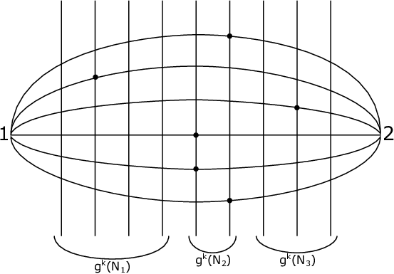
Refer to caption
Figure 6. The case when μ1=6,K11k=4,K12k=2,K13k=3,ρ11=1,ρ12=4,ρ13=1\mu_{1}=6,K_{11}^{k}=4,K_{12}^{k}=2,K_{13}^{k}=3,\rho_{11}=1,\rho_{12}=4,\rho_{13}=1
‖⟨[S~ν],β~∗k​([F~μ])⟩‖≤∑ρ∈M⁡(n,μ,ν)∏i=1n−1μi!​∏j=1n−11ρi​j!​(Ki​jk)ρi​j≤(∏i=1n−1μi)​∑ρ∈M⁡(n,μ,ν)∏i=1n−1∏j=1n−11ρi​j!​(Ak)ρi​j=(∏i=1n−1μi)​(Ak)m​∑ρ∈M⁡(n,μ,ν)∏i=1n−1∏j=1n−11ρi​j!\begin{array}[]{rcl}\left\|\left\langle\left[\widetilde{S}_{\nu}\right],\widetilde{\beta}_{*}^{k}\left(\left[\widetilde{F}_{\mu}\right]\right)\right\rangle\right\|&\leq&\displaystyle{\sum_{\rho\in M(n,\mu,\nu)}\prod_{i=1}^{n-1}\mu_{i}!\prod_{j=1}^{n-1}\frac{1}{\rho_{ij}!}\left(K_{ij}^{k}\right)^{\rho_{ij}}}\\ &\leq&\displaystyle{\left(\prod_{i=1}^{n-1}\mu_{i}\right)\sum_{\rho\in M(n,\mu,\nu)}\prod_{i=1}^{n-1}\prod_{j=1}^{n-1}\frac{1}{\rho_{ij}!}\left(A^{k}\right)^{\rho_{ij}}}\\ &=&\displaystyle{\left(\prod_{i=1}^{n-1}\mu_{i}\right)\left(A^{k}\right)^{m}\sum_{\rho\in M(n,\mu,\nu)}\prod_{i=1}^{n-1}\prod_{j=1}^{n-1}\frac{1}{\rho_{ij}!}}\end{array}

and

Growthk→∞⁡‖⟨[S~ν],β~∗k​([F~μ])⟩‖≤(Growthk→∞⁡Ak)m.\operatorname{\underset{k\to\infty}{\operatorname{Growth}}}\left\|\left\langle\left[\widetilde{S}_{\nu}\right],\widetilde{\beta}_{*}^{k}\left(\left[\widetilde{F}_{\mu}\right]\right)\right\rangle\right\|\leq\left(\operatorname{\underset{k\to\infty}{\operatorname{Growth}}}A^{k}\right)^{m}.

It suffices to show Growthk→∞⁡Ak≤λ\operatorname{\underset{k\to\infty}{\operatorname{Growth}}}A^{k}\leq\lambda. We set

Ui∩g−1​(Uj)=∐l=1Ki​j1Vi​j​lU_{i}\cap g^{-1}(U_{j})=\coprod_{l=1}^{K_{ij}^{1}}V_{ijl}

and take an open cover α={Vi​j​k∣1≤i,j≤n−1,1≤k≤Ki​j1}∪A′\alpha=\{V_{ijk}\mid 1\leq i,j\leq n-1,1\leq k\leq K_{ij}^{1}\}\cup A^{\prime} of the compact set YnY_{n}, where A′A^{\prime} does not contain any intersections of g−1​(αi)g^{-1}(\alpha_{i}) and NjN_{j}.

Lemma 5.3.

Each element of ⋁p=0k−1g−p​(α)\bigvee_{p=0}^{k-1}g^{-p}(\alpha) contains at most one intersection of g−k​(αj)g^{-k}(\alpha_{j}) and NiN_{i}.

Proof.

Every nonempty element of ⋁p=0k−1g−p​(α)\bigvee_{p=0}^{k-1}g^{-p}(\alpha) can be written as

B=Vi0​i1​l1∩⋯∩g−k+1​(Vik−1​ik​lk)B=V_{i_{0}i_{1}l_{1}}\cap\dots\cap g^{-k+1}(V_{i_{k-1}i_{k}l_{k}})

with i0=ii_{0}=i and ik=ji_{k}=j. By the definition of ϕ\phi and ϕ¯\overline{\phi}, gk|B:B→Ujg^{k}|_{B}:B\rightarrow U_{j} is bijective. Therefore (gk|B)−1​(αj)(g^{k}|_{B})^{-1}(\alpha_{j}) is one leaf of UiU_{i} and there exists only one intersection of g−k​(αj)g^{-k}(\alpha_{j}) and NiN_{i}. ∎

It follows from Lemma 5.3 that

Aℓ=∑i,jKi​jℓ≤N⁡(⋁i=0ℓ−1g−i​(α))A^{\ell}=\sum_{i,j}K_{ij}^{\ell}\leq N\left(\bigvee_{i=0}^{\ell-1}g^{-i}(\alpha)\right)

and by (3.1), the growth rate of N⁡(⋁i=0ℓ−1g−i​(α))N\left(\bigvee_{i=0}^{\ell-1}g^{-i}(\alpha)\right) is equal to or less than the dilatation of β\beta. Therefore the proposition follows. ∎

Proposition 5.4.

For any pseudo-Anosov braid β∈Bn\beta\in B_{n}, the inequality

Growthm→∞⁡‖trΓβ,m⁡ζn,m​(β)‖≤λ\operatorname{\underset{m\to\infty}{\operatorname{Growth}}}\left\|\operatorname{tr}_{\Gamma_{\beta,m}}\zeta_{n,m}(\beta)\right\|\leq\lambda

holds.

Proof.

By Lemma 4.3, ‖trΓβk,m⁡ζn,m​(βk)‖\left\|\operatorname{tr}_{\Gamma_{\beta^{k},m}}\zeta_{n,m}(\beta^{k})\right\| is equal to or greater than the number of essential fixed points of g^k\widehat{g}^{k}. For m=1m=1, we notice that g^k\widehat{g}^{k} is gkg^{k}. Therefore ‖trΓβk,1⁡ζn,1​(βk)‖\left\|\operatorname{tr}_{\Gamma_{\beta^{k},1}}\zeta_{n,1}(\beta^{k})\right\| is equal to or greater than the number of essential periodic points of gg whose period is a divisor of kk. In particular, we obtain ‖trΓβk,1⁡ζn,1​(βk)‖≥Dk1/k\left\|\operatorname{tr}_{\Gamma_{\beta^{k},1}}\zeta_{n,1}(\beta^{k})\right\|\geq D_{k}^{1}/\penalty k. Therefore we obtain

‖trΓβ,m⁡ζn,m​(β)‖≤B​#​eFix⁡g^=B​∑(n1,…,nm)∈Am∏i=1m(Di1/ini)≤B​∑(n1,…,nm)∈Am∏i=1m(‖trΓβi,1⁡ζn,1​(βi)‖ni).\begin{array}[]{rcl}\left\|\operatorname{tr}_{\Gamma_{\beta,m}}\zeta_{n,m}(\beta)\right\|&\leq&\displaystyle{B\#\operatorname{eFix}{\widehat{g}}=B\sum_{(n_{1},\dots,n_{m})\in A_{m}}\prod_{i=1}^{m}}\left(\begin{array}[]{c}D_{i}^{1}/\penalty i\\ n_{i}\end{array}\right)\\ &\leq&\displaystyle{B\sum_{(n_{1},\dots,n_{m})\in A_{m}}\prod_{i=1}^{m}}\left(\begin{array}[]{c}\left\|\operatorname{tr}_{\Gamma_{\beta^{i},1}}\zeta_{n,1}(\beta^{i})\right\|\\ n_{i}\end{array}\right).\end{array}

By Proposition 5.2, there exists a monotonically increasing sequence {ai}\{a_{i}\} of real numbers such that

‖trΓβ,1⁡ζn,1​(βi)‖≤(ai​λ)i​and​lim supi→∞ai=1\left\|\operatorname{tr}_{\Gamma_{\beta,1}}\zeta_{n,1}(\beta^{i})\right\|\leq(a_{i}\lambda)^{i}\>\mathrm{and}\>\limsup_{i\to\infty}a_{i}=1

holds. Therefore we obtain

‖trΓβ,m⁡ζn,m​(β)‖≤B​∑(n1,…,nm)∈Am∏i=1m(ai​λ)i​ni≤B​(am​λ)m​Sm,\begin{array}[]{rcl}\left\|\operatorname{tr}_{\Gamma_{\beta,m}}\zeta_{n,m}(\beta)\right\|&\leq&\displaystyle{B\sum_{(n_{1},\dots,n_{m})\in A_{m}}\prod_{i=1}^{m}}(a_{i}\lambda)^{in_{i}}\\ &\leq&\displaystyle{B(a_{m}\lambda)^{m}S_{m}},\end{array}

where SmS_{m} is the number of elements of AmA_{m}.

Lemma 5.5.

The equality limm→∞Sm1/m=1\lim_{m\to\infty}S_{m}^{1/\penalty m}=1 holds.

Proof.

We suppose that m−cm>cm​dmm-c_{m}>c_{m}d_{m}, where

cm=4​(⌊m4⌋+1)2,dm=4​(⌊m4⌋+2)c_{m}=4(\lfloor\sqrt[4]{m}\rfloor+1)^{2},\>d_{m}=4(\lfloor\sqrt[4]{m}\rfloor+2)

and ⌊x⌋\lfloor x\rfloor is the floor function. Let CmC_{m} be the subset of AmA_{m} satisfying the following condition

∑i=1cmni=dm​and​nm−∑i=1cmi​ni=1.\sum_{i=1}^{c_{m}}n_{i}=d_{m}\>\mathrm{and}\>n_{m-\sum_{i=1}^{c_{m}}in_{i}}=1.

Then CmC_{m} is in one-to-one correspondence with the dmd_{m}-combinations with repetition from cmc_{m} elements. Therefore we obtain the inequality

Sm≥(cm+dm−1dm)=(4​(⌊m4⌋+2)​(⌊m4⌋+1)4​(⌊m4⌋+2))=4​(⌊m4⌋+2)​(⌊m4⌋+1)4​(⌊m4⌋+2)×⋯×4​(⌊m4⌋+1)21≥(⌊m4⌋+1)4​(⌊m4⌋+2)≥m44​(⌊m4⌋+2)=m⌊m4⌋+2.\begin{array}[]{rcl}S_{m}&\geq&\left(\begin{array}[]{c}c_{m}+d_{m}-1\\ d_{m}\end{array}\right)=\left(\begin{array}[]{c}4(\lfloor\sqrt[4]{m}\rfloor+2)(\lfloor\sqrt[4]{m}\rfloor+1)\\ 4(\lfloor\sqrt[4]{m}\rfloor+2)\end{array}\right)\\ &=&\displaystyle{\frac{4(\lfloor\sqrt[4]{m}\rfloor+2)(\lfloor\sqrt[4]{m}\rfloor+1)}{4(\lfloor\sqrt[4]{m}\rfloor+2)}\times\dots\times\frac{4(\lfloor\sqrt[4]{m}\rfloor+1)^{2}}{1}}\\ &\geq&\displaystyle{(\lfloor\sqrt[4]{m}\rfloor+1)^{4(\lfloor\sqrt[4]{m}\rfloor+2)}\geq\sqrt[4]{m}^{4(\lfloor\sqrt[4]{m}\rfloor+2)}=m^{\lfloor\sqrt[4]{m}\rfloor+2}}.\end{array}

We set

Am,k={(n1,…,nm)∈Am∣max⁡{i∣ni≠0}=k}.A_{m,k}=\{(n_{1},\dots,n_{m})\in A_{m}\mid\>\max\{i\mid n_{i}\neq 0\}=k\}.

and let Sm,kS_{m,k} be the number of the elements of Am,kA_{m,k}. Then clearly

Sm=∑k=1mSm,kS_{m}=\sum_{k=1}^{m}S_{m,k}

holds and the recursion formula

(5.1) Sm+1,k+1=Sm,k+Sm−k,k+1S_{m+1,k+1}=S_{m,k}+S_{m-k,k+1}

follows from the equality Am,k=∐j=1kAm−k,jA_{m,k}=\coprod_{j=1}^{k}A_{m-k,j}. Moreover, Sm,kS_{m,k} is less than the number of how to put mm balls in distinct kk boxes, which is mkm^{k}.

We assume that maxk⁡Sm,k=Sm,k0\max_{k}S_{m,k}=S_{m,k_{0}}. Since Sm≤m​Sm,k0S_{m}\leq mS_{m,k_{0}} holds, we obtain

mk0≥Sm,k0≥1m​Sm≥mm4m^{k_{0}}\geq S_{m,k_{0}}\geq\frac{1}{m}S_{m}\geq m^{\sqrt[4]{m}}

and k0≥m4k_{0}\geq\sqrt[4]{m}. From (5.1), we obtain

Sm,k0≤S2​(m−k0),m−k0=Sm−k0.S_{m,k_{0}}\leq S_{2(m-k_{0}),m-k_{0}}=S_{m-k_{0}}.

Since SmS_{m} is monotonically increasing for mm, we obtain

Sm≤m​Sm,k0≤m​Sm−k0≤m​Sm−m4.S_{m}\leq mS_{m,k_{0}}\leq mS_{m-k_{0}}\leq mS_{m-\sqrt[4]{m}}.

There exists a natural number NN such that the assumption holds for all m≥Nm\geq N. We set f⁡(m)=m−m4f(m)=m-\sqrt[4]{m} and nN​(m)=min⁡{i∣fi​(m)≤N}n_{N}(m)=\min\{i\mid f^{i}(m)\leq N\}. Then we obtain Sm≤mnN​(m)​SNS_{m}\leq m^{n_{N}(m)}S_{N}. We notice that if xx is larger than (m4−1)4(\sqrt[4]{m}-1)^{4}, then x−f⁡(x)=x4x-f(x)=\sqrt[4]{x} is larger than m4−1\sqrt[4]{m}-1. Therefore we obtain

f⌊m42−2​m4+2⌋+1​(m)≤m−(m4+(m4−1)​(m42−2​m4+2))=(m4−1)4.f^{\lfloor\sqrt[4]{m}^{2}-2\sqrt[4]{m}+2\rfloor+1}(m)\leq m-(\sqrt[4]{m}+(\sqrt[4]{m}-1)(\sqrt[4]{m}^{2}-2\sqrt[4]{m}+2))=(\sqrt[4]{m}-1)^{4}.

Therefore we obtain

nN​(m)≤∑k=1m4⌊4​k2−2​k+2⌋+1≤m4​(4​m42−2​m4+3)≤4​m3/4n_{N}(m)\leq\sum_{k=1}^{\sqrt[4]{m}}\lfloor 4k^{2}-2k+2\rfloor+1\leq\sqrt[4]{m}(4\sqrt[4]{m}^{2}-2\sqrt[4]{m}+3)\leq 4m^{3/\penalty 4}

and

1<Smm≤(mnN​(m)​SfnN​(m)​(m))1/m≤SNm​m4​m−14.1<\sqrt[m]{S_{m}}\leq(m^{n_{N}(m)}S_{f^{n_{N}(m)}(m)})^{1/\penalty m}\leq\sqrt[m]{S_{N}}m^{4m^{-\frac{1}{4}}}.

Since the limit limm→∞SNm​m4/m4\lim_{m\to\infty}\sqrt[m]{S_{N}}m^{4/\penalty\sqrt[4]{m}} equals 1, squeeze theorem leads to the conclusion limm→∞Sm1/m=1\lim_{m\to\infty}S_{m}^{1/\penalty m}=1. ∎

By this lemma, we obtain

lim supm→∞‖trΓβ,m⁡ζn,m​(β)‖1/m≤lim supm→∞(B​Sm)1/m​am​λ=λ.\limsup_{m\to\infty}\left\|\operatorname{tr}_{\Gamma_{\beta,m}}\zeta_{n,m}(\beta)\right\|^{1/\penalty m}\leq\limsup_{m\to\infty}(BS_{m})^{1/\penalty m}a_{m}\lambda=\lambda.

∎

Proof of Theorem 1.1. Since we have the inequality tr⁡(‖A‖)≥‖tr⁡A‖\operatorname{tr}(\left\|A\right\|)\geq\left\|\operatorname{tr}A\right\| for any matrix AA with coefficients in Laurent polynomial ring, we obtain

λm≤Growthk→∞⁡‖trΓβk,m⁡ζn,m​(βk)‖≤Growthk→∞⁡tr⁡‖ζn,m​(βk)‖≤λm\lambda^{m}\leq\operatorname{\underset{k\to\infty}{\operatorname{Growth}}}\left\|\operatorname{tr}_{\Gamma_{\beta^{k},m}}\zeta_{n,m}(\beta^{k})\right\|\leq\operatorname{\underset{k\to\infty}{\operatorname{Growth}}}\operatorname{tr}\left\|\zeta_{n,m}(\beta^{k})\right\|\leq\lambda^{m}

by Proposition 5.1 and Proposition 5.2. Therefore we have

Growthk→∞⁡‖trΓβk,m⁡ζn,m​(βk)‖=Growthk→∞⁡tr⁡‖ζn,m​(βk)‖=λm.\operatorname{\underset{k\to\infty}{\operatorname{Growth}}}\left\|\operatorname{tr}_{\Gamma_{\beta^{k},m}}\zeta_{n,m}(\beta^{k})\right\|=\operatorname{\underset{k\to\infty}{\operatorname{Growth}}}\operatorname{tr}\left\|\zeta_{n,m}(\beta^{k})\right\|=\lambda^{m}.

We have

λ≤Growthm→∞⁡‖trΓβ,m⁡ζn,m​(β)‖≤λ\lambda\leq\operatorname{\underset{m\to\infty}{\operatorname{Growth}}}\left\|\operatorname{tr}_{\Gamma_{\beta,m}}\zeta_{n,m}(\beta)\right\|\leq\lambda

by Proposition 5.1 and Proposition 5.4 and we have Growthm→∞⁡‖trΓβ,m⁡ζn,m​(β)‖=λ\operatorname{\underset{m\to\infty}{\operatorname{Growth}}}\left\|\operatorname{tr}_{\Gamma_{\beta,m}}\zeta_{n,m}(\beta)\right\|=\lambda. □\Box

6. Homological representation of braid groups

6.1. Homological representation of braid groups

In [20] Lawrence construct a monodromy representation of braid groups. We review the representation. We take a homomorphism

ρB:𝐁n,1​(D2)≅⟨σ1,…,σn−1,σn2⟩→ℤ\rho_{B}:{\bf B}_{n,1}(D^{2})\cong\langle\sigma_{1},\dots,\sigma_{n-1},\sigma_{n}^{2}\rangle\rightarrow\mathbb{Z}

defined by ρB​(σi)=0\rho_{B}(\sigma_{i})=0 for all 1≤i<n1\leq i<n and ρB​(σn2)=1\rho_{B}(\sigma_{n}^{2})=1. Let pB:Dn~B→Dnp_{B}:\widetilde{D_{n}}^{B}\rightarrow D_{n} be the covering corresponding to Ker⁡ρB\operatorname{Ker}\rho_{B} and fix d~B∈pB−1​(d1)\widetilde{d}^{B}\in p_{B}^{-1}(d_{1}). For an nn-braid β\beta, we take a representative ff. Let

f~B:(Dn~B,d~B)→(Dn~B,d~B)\widetilde{f}^{B}:(\widetilde{D_{n}}^{B},\widetilde{d}^{B})\rightarrow(\widetilde{D_{n}}^{B},\widetilde{d}^{B})

be the lift of ff. Then f~B\widetilde{f}^{B} acts on H1​(Dn~B,∂Dn~B)H_{1}(\widetilde{D_{n}}^{B},\partial\widetilde{D_{n}}^{B}) as ℤ⁡[ℤ]\mathbb{Z}[\mathbb{Z}]-homomorphism. The linear representation BB defined by B⁡(β)=f~∗BB(\beta)=\widetilde{f}^{B}_{*} is called the reduced Burau representation. Let tt denote the generator of covering transformation of Dn~B\widetilde{D_{n}}^{B} corresponding to 1∈ℤ1\in\mathbb{Z}. Then the ring ℤ⁡[ℤ]\mathbb{Z}[\mathbb{Z}] is isomorphic to the Laurent polynomial ring ℤ⁡[t±1]\mathbb{Z}[t^{\pm 1}] and B⁡(β)B(\beta) can be regarded as a matrix with coefficients in the Laurent polynomial ring ℤ⁡[t±1]\mathbb{Z}[t^{\pm 1}]. Similarly for m≥2m\geq 2, we take a homomorphism

ρ𝐿𝐾𝐵:𝐁n,m​(D2)≅⟨σ1,…,σn−1,σn2,σn+1,…,σn+m−1⟩→ℤ⊕ℤ\rho_{\mathit{LKB}}:{\bf B}_{n,m}(D^{2})\cong\langle\sigma_{1},\dots,\sigma_{n-1},\sigma_{n}^{2},\sigma_{n+1},\dots,\sigma_{n+m-1}\rangle\rightarrow\mathbb{Z}\oplus\mathbb{Z}

defined by ρ𝐿𝐾𝐵​(σi)=0⊕0\rho_{\mathit{LKB}}(\sigma_{i})=0\oplus 0 for all 1≤i<n1\leq i<n, ρ𝐿𝐾𝐵​(σn2)=1⊕0\rho_{\mathit{LKB}}(\sigma_{n}^{2})=1\oplus 0 and ρ𝐿𝐾𝐵​(σn+j)=0⊕1\rho_{\mathit{LKB}}(\sigma_{n+j})=0\oplus 1 for all 1≤j<m1\leq j<m. Let p𝐿𝐾𝐵:𝒞~n,m𝐿𝐾𝐵​(D2)→𝒞n,m​(D2)p_{\mathit{LKB}}:\widetilde{\mathcal{C}}^{\mathit{LKB}}_{n,m}(D^{2})\rightarrow\mathcal{C}_{n,m}(D^{2}) be the covering corresponding to Ker⁡ρ𝐿𝐾𝐵\operatorname{Ker}\rho_{\mathit{LKB}} and fix c~𝐿𝐾𝐵∈p𝐿𝐾𝐵−1​(c)\widetilde{c}^{\mathit{LKB}}\in p_{\mathit{LKB}}^{-1}(c). For β∈Bn\beta\in B_{n}, we take a representative ff. Let

f~𝐿𝐾𝐵:(𝒞~n,m𝐿𝐾𝐵​(D2),c~𝐿𝐾𝐵)→(𝒞~n,m𝐿𝐾𝐵​(D2),c~𝐿𝐾𝐵)\widetilde{f}^{\mathit{LKB}}:(\widetilde{\mathcal{C}}^{\mathit{LKB}}_{n,m}(D^{2}),\widetilde{c}^{\mathit{LKB}})\rightarrow(\widetilde{\mathcal{C}}^{\mathit{LKB}}_{n,m}(D^{2}),\widetilde{c}^{\mathit{LKB}})

be the lift of f^\widehat{f}. Then f~𝐿𝐾𝐵\widetilde{f}^{\mathit{LKB}} acts on H2​(B~n,m𝐿𝐾𝐵​(D2))H_{2}(\widetilde{B}^{\mathit{LKB}}_{n,m}(D^{2})) as an ℤ⁡[ℤ⊕ℤ]\mathbb{Z}[\mathbb{Z}\oplus\mathbb{Z}]-homomorphism. The linear representation 𝐿𝐾𝐵m\mathit{LKB}_{m} defined by 𝐿𝐾𝐵m​(β)=f~∗𝐿𝐾𝐵\mathit{LKB}_{m}(\beta)=\widetilde{f}^{\mathit{LKB}}_{*} is called the Lawrence-Krammer-Bigelow representations. Let qq and tt denote the generator of covering transformation of 𝒞~n,m𝐿𝐾𝐵​(D2)\widetilde{\mathcal{C}}^{\mathit{LKB}}_{n,m}(D^{2}) corresponding to 1⊕0∈ℤ⊕ℤ1\oplus 0\in\mathbb{Z}\oplus\mathbb{Z} and 0⊕1∈ℤ⊕ℤ0\oplus 1\in\mathbb{Z}\oplus\mathbb{Z} respectively. Then the ring ℤ⁡[ℤ⊕ℤ]\mathbb{Z}[\mathbb{Z}\oplus\mathbb{Z}] is isomorphic to the Laurent polynomial ring ℤ⁡[q±1,t±1]\mathbb{Z}[q^{\pm 1},t^{\pm 1}] and 𝐿𝐾𝐵m​(β)\mathit{LKB}_{m}(\beta) can be regarded as a matrix with coefficients in the 2-variable Laurent polynomial ring ℤ⁡[q±1,t±1]\mathbb{Z}[q^{\pm 1},t^{\pm 1}].

The homological representation of braid groups has been also intensively studied. The Lawrence-Krammer-Bigelow representations of the braid groups were studied by Lawrence [20] in relation with Hecke algebra representations of the braid groups. In [4], [18] and [19], Bigelow and Krammer showed the faithfulness of the Lawrence-Krammer-Bigelow representation for m=2m=2 independently.

In [8], Fried showed how to estimate the entropy of a pseudo-Anosov braid by using the Burau matrix B⁡(t)B(t) of a pseudo-Anosov braid. In [17], Kolev proved the same estimation directly with different methods. The following theorem is the estimate and this estimate is called the Burau estimate.

Theorem 6.1.

(Fried [8], Kolev [17]) Let ff be a homeomorphism of D2D^{2} fixing PnP_{n} setwise and β\beta be an nn-braid represented by ff. Then the topological entropy of ff is equal to or greater than the logarithm of the spectral radius of the Burau matrix B⁡(t)B(t) of β\beta after substituting a complex number of modulus 1 in place of tt.

If the inequality is an equality for η=η0\eta=\eta_{0}, then the Burau estimate is said to be sharp at η0\eta_{0}. In [2], Band and Boyland determined a necessary and sufficient condition when the Burau estimate is sharp at the root of unity.

Theorem 6.2.

(Band and Boyland [2]) For a pseudo-Anosov braid β\beta, the Burau estimate is sharp at the root of unity η0\eta_{0} only if η0=−1\eta_{0}=-1. Furthermore, the Burau estimate is sharp at −1-1 if and only if the invariant foliations for a pseudo-Anosov map in the class represented by β\beta have odd order singularities at all punctures and all interior singularities are even order.

In [16], Koberda shows the similar estimate by using Lawrence-Krammer-Bigelow representation.

Theorem 6.3.

(Koberda [16]) For a pseudo-Anosov braid β\beta, the mm-th power of the dilatation of β\beta is equal to or greater than the spectral radius of the Lawrence-Krammer-Bigelow matrix 𝐿𝐾𝐵m​(q,t)\mathit{LKB}_{m}(q,t) of β\beta after substituting complex numbers of modulus 1 in place of qq and tt.

6.2. Homological estimation and Theorem 1.1

In this section, we recover the estimation in [8], [17] and [16] using Theorem 1.1. If we have a homomorphism ρ\rho from 𝐄n,m​(D2){\bf E}_{n,m}(D^{2}) to some group GG, we have an another representation ρ∗​(ζn,m)\rho_{*}(\zeta_{n,m}) on the free ℤ⁡[G]\mathbb{Z}[G]-module defined by ρ∗​(ζn,m)=(ρ∗​(cμ​ν(β)))\rho_{*}(\zeta_{n,m})=(\rho_{*}(c_{\mu\nu}^{(\beta)})). Moreover, if GG is a finitely generated free abelian group, ℤ⁡[G]\mathbb{Z}[G] can be embedded in ℂ\mathbb{C} and in this way, ρ∗​(ζn,m)\rho_{*}(\zeta_{n,m}) gives rise to a linear representation ρ∗′​(ζn,m)\rho_{*}^{\prime}(\zeta_{n,m}) over ℂ\mathbb{C}.

When m=1m=1, Let ρB′:𝐄n,1​(D2)→ℤ\rho_{B}^{\prime}:{\bf E}_{n,1}(D^{2})\rightarrow\mathbb{Z} be a the homomorphism defined by ρB′​(σi)=0\rho_{B}^{\prime}(\sigma_{i})=0 for all 1≤i<n1\leq i<n and ρB′​(σi2)=1\rho_{B}^{\prime}(\sigma_{i}^{2})=1. When m≥2m\geq 2, let ρ𝐿𝐾𝐵′:𝐄n,m​(D2)→ℤ⊕ℤ\rho_{\mathit{LKB}}^{\prime}:{\bf E}_{n,m}(D^{2})\rightarrow\mathbb{Z}\oplus\mathbb{Z} be a homomorphism defined by ρ𝐿𝐾𝐵′​(σi)=0⊕0\rho_{\mathit{LKB}}^{\prime}(\sigma_{i})=0\oplus 0 for all 1≤i<n1\leq i<n, ρ𝐿𝐾𝐵′​(σn2)=1⊕0\rho_{\mathit{LKB}}^{\prime}(\sigma_{n}^{2})=1\oplus 0 and ρ𝐿𝐾𝐵′​(σn+j)=0⊕1\rho_{\mathit{LKB}}^{\prime}(\sigma_{n+j})=0\oplus 1. We consider the homomorphism from AutR⁡(R⊗RBℋF)\operatorname{Aut}_{R}\left(R\otimes_{R_{B}}\mathcal{H}_{F}\right) induced by ρ𝐿𝐾𝐵′\rho_{\mathit{LKB}}^{\prime}. Since ρ𝐿𝐾𝐵′​(σi)\rho_{\mathit{LKB}}^{\prime}(\sigma_{i}) is 0⊕00\oplus 0 for all 1≤i<n1\leq i<n, the action as the right multiplication becomes trivial and (ρ𝐿𝐾𝐵′)∗​(ζn,m)(\rho_{\mathit{LKB}}^{\prime})_{*}(\zeta_{n,m}) is equivalent to the Lawrence-Krammer-Bigelow representations for all m≥2m\geq 2. Similarly, (ρB′)∗​(ζn,m)(\rho_{B}^{\prime})_{*}(\zeta_{n,m}) is equivalent to the reduced Burau representation.

For any matrix AA with coefficients in nn-variable Laurent polynomial ring and complex numbers x1,…,xnx_{1},\dots,x_{n}, we denote by A⁡(x1,…,xn)A(x_{1},\dots,x_{n}) the matrix with coefficients in ℂ\mathbb{C} substituting xix_{i} for ii-th variable. For any matrix AA with coefficients in ℂ\mathbb{C}, we denote by sr⁡A\operatorname{sr}A the spectral radius of AA. We state the main result of this section.

Proposition 6.4.

For any matrix AA with coefficients in the Laurent polynomial ring ℤ⁡[x1,…,xn]\mathbb{Z}[x_{1},\dots,x_{n}], we have

Growthk→∞⁡‖tr⁡Ak‖=supxi∈S1sr⁡A⁡(x1,…,xn).\operatorname{\underset{k\to\infty}{\operatorname{Growth}}}\left\|\operatorname{tr}A^{k}\right\|=\sup_{x_{i}\in S^{1}}\operatorname{sr}A(x_{1},\dots,x_{n}).

Let I=(i1,…,in)I=(i_{1},\dots,i_{n}) be a multi index and xI=∏k=0nxkikx^{I}=\prod_{k=0}^{n}x_{k}^{i_{k}}.

Lemma 6.5.

We suppose f⁡(x1,…,xn)=∑i1=0M…​∑in=0MaI​xIf(x_{1},\dots,x_{n})=\sum_{i_{1}=0}^{M}\dots\sum_{i_{n}=0}^{M}a_{I}x^{I} is an nn-variable polynomial of degree MM. Then we have the inequality

∑I|aI|≤(M+1)n​supxk∈S1|f⁡(x1,…,xn)|\sum_{I}|a_{I}|\leq(M+1)^{n}\sup_{x_{k}\in S^{1}}|f(x_{1},\dots,x_{n})|
Proof.

First of all, we prove the case n=1n=1. Then f⁡(x)f(x) is a polynomial ∑i=0Mai​xi\sum_{i=0}^{M}a_{i}x^{i} of degree MM. We consider the Vandermonde matrix

V=VM+1​(x0,…,xM)=(1x0⋯x0M1x1⋯x1M⋮⋮⋱⋮1xM⋯xMM).V=V_{M+1}(x_{0},\dots,x_{M})=\left(\begin{array}[]{cccc}1&x_{0}&\cdots&x_{0}^{M}\\ 1&x_{1}&\cdots&x_{1}^{M}\\ \vdots&\vdots&\ddots&\vdots\\ 1&x_{M}&\cdots&x_{M}^{M}\\ \end{array}\right).

Then we have V​𝐚=𝐀V{\bf a}={\bf A}, where

𝐚=(a0⋮aM)​and​𝐀=(f⁡(x0)⋮f⁡(xM)).{\bf a}=\left(\begin{array}[]{c}a_{0}\\ \vdots\\ a_{M}\end{array}\right)\mathrm{\>and\>}{\bf A}=\left(\begin{array}[]{c}f(x_{0})\\ \vdots\\ f(x_{M})\end{array}\right).

We denote by σm\sigma_{m} the mm-th elementary symmetric function in the (M+1)(M+1) variables x0,…,xMx_{0},\dots,x_{M}. In other words, we have

σm=σm​(x0,…,xM)=∑ν∈𝒮mxν⁡(1)​…​xν⁡(m)\sigma_{m}=\sigma_{m}(x_{0},\dots,x_{M})=\sum_{\nu\in\mathcal{S}_{m}}x_{\nu(1)}\dots x_{\nu(m)}

for all 1≤m≤M+11\leq m\leq M+1 and σ0=1\sigma_{0}=1. We use the notation σmi\sigma_{m}^{i} to denote the mm-th elementary symmetric function in the MM variables xkx_{k} with xix_{i} missing. In other words, we have

σmi=σm​(x0,…,xi−1,xi+1,…,xM).\sigma_{m}^{i}=\sigma_{m}(x_{0},\dots,x_{i-1},x_{i+1},\dots,x_{M}).

We set V−1=(vi​j)0≤i,j≤MV^{-1}=(v_{ij})_{0\leq i,j\leq M}. It is well known (see [9]) that we have

vi​j=(−1)i​σM−ij∏k≠j(xk−xj)v_{ij}=(-1)^{i}\frac{\sigma_{M-i}^{j}}{\prod_{k\neq j}(x_{k}-x_{j})}

We put θ=π/M+1\theta=\pi/\penalty M+1 and xk=exp⁡(2​−1​k​θ)x_{k}=\exp(2\sqrt{-1}k\theta). Since xix_{i}’s are all the roots of zM+1−1=0z^{M+1}-1=0, we obtain σm​(x0,…,xM)=0\sigma_{m}(x_{0},\dots,x_{M})=0 for all 1≤m≤M1\leq m\leq M. Since the recursion formula σm+1i=σm+1−xi​σmi\sigma_{m+1}^{i}=\sigma_{m+1}-x_{i}\sigma_{m}^{i} holds, we obtain σm+1i=−xi​σmi\sigma_{m+1}^{i}=-x_{i}\sigma_{m}^{i} and σmi=(−xi)m\sigma_{m}^{i}=(-x_{i})^{m}. Then we obtain

|vi​j|=|(−1)i−1​σM−ij∏k≠j(xk−xj)|=1∏k=1M(2​sin⁡k​θ).|v_{ij}|=\left|(-1)^{i-1}\frac{\sigma_{M-i}^{j}}{\prod_{k\neq j}(x_{k}-x_{j})}\right|=\frac{1}{\prod_{k=1}^{M}(2\sin k\theta)}.

Since we have 𝐚=V−1​𝐀{\bf a}=V^{-1}{\bf A}, we have the inequality

|ai|≤M+1∏k=1M(2​sin⁡k​θ)​maxk​|f⁡(xk)|≤M+1∏k=1M(2​sin⁡k​θ)​supx∈S1|f⁡(x)|.|a_{i}|\leq\frac{M+1}{\prod_{k=1}^{M}(2\sin k\theta)}\max_{k}\left|f(x_{k})\right|\leq\frac{M+1}{\prod_{k=1}^{M}(2\sin k\theta)}\sup_{x\in S^{1}}\left|f(x)\right|.
Lemma 6.6.

The equality ∏k=1M(2​sin⁡k​θ)=M+1\prod_{k=1}^{M}(2\sin k\theta)=M+1 holds.

Proof.

We set

cos⁡(2​n−1)​θ=cos⁡θ​fn​(cos⁡θ),sin⁡2​n​θ=sin⁡2​θ​gn​(cos⁡θ)\cos(2n-1)\theta=\cos\theta f_{n}(\cos\theta),\>\sin 2n\theta=\sin 2\theta g_{n}(\cos\theta)

for n≥1n\geq 1. Since

{cos⁡(2​n+3)​θ+cos⁡(2​n−1)​θ=2​cos⁡2​θ​cos⁡(2​n+1)​θsin⁡2​(n+2)​θ+sin⁡2​n​θ=2​cos⁡2​θ​sin⁡2​(n+1)​θ,\left\{\begin{array}[]{l}\cos(2n+3)\theta+\cos(2n-1)\theta=2\cos 2\theta\cos(2n+1)\theta\\ \sin 2(n+2)\theta+\sin 2n\theta=2\cos 2\theta\sin 2(n+1)\theta,\end{array}\right.

hold, we obtain recursion formulae fn+2​(x)=2​(2​x2−1)​fn+1​(x)−fn​(x)f_{n+2}(x)=2(2x^{2}-1)f_{n+1}(x)-f_{n}(x) and gn+2​(x)=2​(2​x2−1)​gn+1​(x)−gn​(x)g_{n+2}(x)=2(2x^{2}-1)g_{n+1}(x)-g_{n}(x). Moreover, because of the initial conditions f1​(x)=1f_{1}(x)=1, f2​(x)=4​x2−3f_{2}(x)=4x^{2}-3, g1​(x)=1g_{1}(x)=1 and g2​(x)=4​x2−2g_{2}(x)=4x^{2}-2, fn​(x)f_{n}(x) and gn​(x)g_{n}(x) are polynomials of degree 2​(n−1)2(n-1). Solving the recursion formulae of leading coefficient and constant term, we find that the leading coefficients of fn​(x)f_{n}(x) and gn​(x)g_{n}(x) is 4n4^{n}, the constant term of fn​(x)f_{n}(x) is (2​n−1)​(−1)n−1(2n-1)(-1)^{n-1} and the constant term of gn​(x)g_{n}(x) is n​(−1)n−1n(-1)^{n-1}.

There exist distinct 2​(n−1)2(n-1) solutions

±sin⁡(k​π/(2​n−1))=cos⁡(π/2±k​π/(2​n−1))​k=1,…,n−1\pm\sin(k\pi/\penalty(2n-1))=\cos(\pi/2\pm k\pi/\penalty(2n-1))\>\>k=1,\dots,n-1

of fn​(x)=0f_{n}(x)=0 and distinct 2​(n−1)2(n-1) solutions

±sin⁡(k​π/2​n)=cos⁡(π/2±k​π/2​n)​k=1,…,n−1\pm\sin(k\pi/\penalty 2n)=\cos(\pi/2\pm k\pi/\penalty 2n)\>\>k=1,\dots,n-1

of gn​(x)=0g_{n}(x)=0. Vieta’s formula implies ∏k=1M(2​sin⁡k​θ)=M+1\prod_{k=1}^{M}(2\sin k\theta)=M+1. ∎

Lemma 6.6 implies ∑i=0M|ai|≤(M+1)​supx∈S1|f⁡(x)|\sum_{i=0}^{M}|a_{i}|\leq(M+1)\sup_{x\in S^{1}}|f(x)|.

Now we consider the general case. For any nn-variable polynomial

f⁡(x1,…,xn)=∑i1=0M…​∑in=0MaI​xIf(x_{1},\dots,x_{n})=\sum_{i_{1}=0}^{M}\dots\sum_{i_{n}=0}^{M}a_{I}x^{I}

of degree MM, we set

f⁡(x1,…,xn)=∑in=0Mfin​(x1,…,xn−1)​xnin.f(x_{1},\dots,x_{n})=\sum_{i_{n}=0}^{M}f_{i_{n}}(x_{1},\dots,x_{n-1})x_{n}^{i_{n}}.

Then we obtain

supx1,…,xn−1∈S1∑i|fi​(x1,…,xn−1)|≤(M+1)​supx1,…,xn∈S1|f⁡(x1,…,xn)|.\sup_{x_{1},\dots,x_{n-1}\in S^{1}}\sum_{i}|f_{i}(x_{1},\dots,x_{n-1})|\leq(M+1)\sup_{x_{1},\dots,x_{n}\in S^{1}}|f(x_{1},\dots,x_{n})|.

Repeating this nn times shows the inequality

∑I|aI|≤(M+1)n​supx1,…,xn∈S1|f⁡(x1,…,xn)|.\sum_{I}|a_{I}|\leq(M+1)^{n}\sup_{x_{1},\dots,x_{n}\in S^{1}}|f(x_{1},\dots,x_{n})|.

∎

Proof of Proposition 6.4. We notice that

supxi∈S1|∑i1=mM…​∑in=mMaI​xI|=supxi∈S1|∑i1=0M−m…​∑in=0M−maI​xI|\sup_{x_{i}\in S^{1}}\left|\sum_{i_{1}=m}^{M}\dots\sum_{i_{n}=m}^{M}a_{I}x^{I}\right|=\sup_{x_{i}\in S^{1}}\left|\sum_{i_{1}=0}^{M-m}\dots\sum_{i_{n}=0}^{M-m}a_{I}x^{I}\right|

holds. We denote by AA a matrix with coefficients in nn-variable Laurent polynomial ring. Let MM and mm be the maximum and minimum degree of all entries of AA. Then the maximum degree of all entries of AkA^{k} is equal to or less than k​MkM and the minimum degree of all entries of AkA^{k} is equal to or greater than k​mkm. Using Lemma 6.5, we obtain

supxi∈S1|tr⁡Ak​(x1,…,xn)|≤‖tr⁡Ak‖≤(k⁡(M−m)+1)n​supxi∈S1|tr⁡Ak​(x1,…,xn)|.\sup_{x_{i}\in S^{1}}|\operatorname{tr}A^{k}(x_{1},\dots,x_{n})|\leq\left\|\operatorname{tr}A^{k}\right\|\leq(k(M-m)+1)^{n}\sup_{x_{i}\in S^{1}}|\operatorname{tr}A^{k}(x_{1},\dots,x_{n})|.

Therefore we obtain

Growthk→∞‖trAk‖=Growthk→∞supxi∈S1|trAk(x1,…,xn)|.\operatorname{\underset{k\to\infty}{\operatorname{Growth}}}\left\|\operatorname{tr}A^{k}\right\|=\operatorname{\underset{k\to\infty}{\operatorname{Growth}}}\sup_{x_{i}\in S^{1}}|\operatorname{tr}A^{k}(x_{1},\dots,x_{n})|.

Cayley-Hamilton theorem shows

tr⁡Ak​(x1,…,xn)=λ1k+⋯+λNk,\operatorname{tr}A^{k}(x_{1},\dots,x_{n})=\lambda_{1}^{k}+\dots+\lambda_{N}^{k},

where λ1,…,λN\lambda_{1},\dots,\lambda_{N} are the eigenvalues of A⁡(x1,…,xn)A(x_{1},\dots,x_{n}). Therefore we obtain

Growthk→∞supxi∈S1|trAk(x1,…,xn)|=supxi∈S1srA(x1,…,xn).\operatorname{\underset{k\to\infty}{\operatorname{Growth}}}\sup_{x_{i}\in S^{1}}|\operatorname{tr}A^{k}(x_{1},\dots,x_{n})|=\sup_{x_{i}\in S^{1}}\operatorname{sr}A(x_{1},\dots,x_{n}).

□\Box

Using Proposition 6.4, we recover the estimation in [8], [17] and [16].

Corollary 6.7.

For a pseudo-Anosov braid β\beta, the dilatation of β\beta is equal to or greater than the spectral radius of the Burau matrix B⁡(t)B(t) of β\beta after substituting a complex number of modulus 1 in place of tt and the mm-th power of the dilatation of β\beta is equal to or greater than the spectral radius of the Lawrence-Krammer-Bigelow matrix 𝐿𝐾𝐵m​(q,t)\mathit{LKB}_{m}(q,t) of β\beta after substituting complex numbers of modulus 1 in place of qq and tt.

Proof.

Since ‖tr⁡(ρ)∗​(ζn,m)​(βk)‖\left\|\operatorname{tr}(\rho)_{*}(\zeta_{n,m})(\beta^{k})\right\| is equal to or less than ‖trΓβk,m⁡ζn,m​(βk)‖\left\|\operatorname{tr}_{\Gamma_{\beta^{k},m}}\zeta_{n,m}(\beta^{k})\right\|, we obtain

Growthk→∞⁡‖tr⁡(ρB′)∗​(ζn,1)​(βk)‖≤λ\operatorname{\underset{k\to\infty}{\operatorname{Growth}}}\left\|\operatorname{tr}(\rho_{B}^{\prime})_{*}(\zeta_{n,1})(\beta^{k})\right\|\leq\lambda

and

Growthk→∞⁡‖tr⁡(ρ𝐿𝐾𝐵′)∗​(ζn,m)​(βk)‖≤λm.\operatorname{\underset{k\to\infty}{\operatorname{Growth}}}\left\|\operatorname{tr}(\rho_{\mathit{LKB}}^{\prime})_{*}(\zeta_{n,m})(\beta^{k})\right\|\leq\lambda^{m}.

From Proposition 6.4, we obtain

Growthk→∞⁡‖tr⁡(ρB′)∗​(ζn,1)​(βk)‖=supt∈S1B⁡(t)\operatorname{\underset{k\to\infty}{\operatorname{Growth}}}\left\|\operatorname{tr}(\rho_{B}^{\prime})_{*}(\zeta_{n,1})(\beta^{k})\right\|=\sup_{t\in S^{1}}B(t)

and

Growthk→∞⁡‖tr⁡(ρ𝐿𝐾𝐵′)∗​(ζn,m)​(βk)‖=supq,t∈S1𝐿𝐾𝐵m​(q,t).\operatorname{\underset{k\to\infty}{\operatorname{Growth}}}\left\|\operatorname{tr}(\rho_{\mathit{LKB}}^{\prime})_{*}(\zeta_{n,m})(\beta^{k})\right\|=\sup_{q,t\in S^{1}}\mathit{LKB}_{m}(q,t).

Therefore we obtain

supt∈S1B⁡(t)≤λ​and​supq,t∈S1𝐿𝐾𝐵m​(q,t)≤λm.\sup_{t\in S^{1}}B(t)\leq\lambda\mathrm{\>\>\>and\>}\sup_{q,t\in S^{1}}\mathit{LKB}_{m}(q,t)\leq\lambda^{m}.

∎

On the other hand, it is not known whether Growthm→∞⁡‖tr⁡(ρ𝐿𝐾𝐵)∗​(ζn,m)​(β)‖\operatorname{\underset{m\to\infty}{\operatorname{Growth}}}\left\|\operatorname{tr}(\rho_{\mathit{LKB}})_{*}(\zeta_{n,m})(\beta)\right\| is λ\lambda or not. If Growthm→∞⁡‖tr⁡(ρ𝐿𝐾𝐵)∗​(ζn,m)​(β)‖\operatorname{\underset{m\to\infty}{\operatorname{Growth}}}\left\|\operatorname{tr}(\rho_{\mathit{LKB}})_{*}(\zeta_{n,m})(\beta)\right\| is not necessarily λ\lambda, there exists some sufficient condition for Growthm→∞⁡‖tr⁡(ρ𝐿𝐾𝐵)∗​(ζn,m)​(β)‖=λ\operatorname{\underset{m\to\infty}{\operatorname{Growth}}}\left\|\operatorname{tr}(\rho_{\mathit{LKB}})_{*}(\zeta_{n,m})(\beta)\right\|=\lambda. Clearly the condition in Theorem 6.2 is a sufficient condition for the above equality. We want to reveal whether this sufficient condition is the best condition or not.

Acknowledgement

I would like to show my greatest appreciation to Professor Toshitake Kohno whose comments and suggestions were of inestimable value for my study. Special thanks also go to the member of the same seninar whose opinions and information have helped me very much throughout the production of this study. I would also like to express my gratitude to my family for their moral support and warm encouragements.

References

  • [1] R. L. Adler, A. G. Konheim and M. H. McAndrew, Topological entropy, Trans. Amer. Math. Soc. 114 (1965), 309-319.
  • [2] G. Band and P. Boyland, The Burau estimate for the entropy of a braid, Algebr. Geom. Topol. 7 (2007), 1345-1378.
  • [3] M. Bestvina and M. Handel, Train-tracks for surface homeomorphisms, Topology 34 (1995), no. 1, 109-140.
  • [4] S. Bigelow, Braid groups are linear, J. Amer. Math. Soc. 14 (2001), 471-486.
  • [5] S. Bigelow, A homological definition of the Jones polynomial, Geom. Topol. Monogr. 4 (2002), 29-41.
  • [6] S. Bigelow, The Lawrence-Krammer representation, Topology and geometry of manifolds (Athens, GA, 2001), 51-68, Proc. Sympos. Pure Math., 71, Amer. Math. Soc., Providence, RI, 2003.
  • [7] A. Fathi, F. Laudenbach and V. Poénaru, Travaux de Thurston sur les surfaces, Séminaire Orsay, Astérisque, vol. 66-67, Soc. Math. France, Paris, (1979).
  • [8] D. Fried, Entropy and twisted cohomology, Topology 25 (1986), 455-470.
  • [9] W. Galitschi, On inverses of Vandermonde and confluent Vandermonde matrices, Numerische Mathematik 4 (1962), 117-123.
  • [10] N.V. Ivanov, Entropy and the Nielsen numbers, Soviet Math. DokL, 26 (1982), 63-66.
  • [11] B. Jiang, Lectures on Nielsen Fixed Point Theory, Contemp. Math., vol. 14, Amer. Math. Soc, Providence, 1983.
  • [12] B. Jiang, A characterization of fixed point classes, Fixed Point Theory and its Applications, (R.F. Brown ed.), Contemp. Math., vol. 72, Amer. Math. Soc, Providence, 1988, 157-160.
  • [13] B. Jiang, Estimation of the number of periodic orbits, Pacific J. Math. Volume 172, Number 1 (1996), 151-185.
  • [14] B. Jiang and H. Zheng, A trace formula for the forcing relation of braids, Topology 47 (2008), 51-70.
  • [15] B. Jiang, X. Zhao and H. Zheng, On fixed points of stratified maps, Journal of Fixed Point Theory and Applications 2.2 (2007), 225-240.
  • [16] T. Koberda, Asymptotic linearity of the mapping class group and a homological version of the Nielsen–Thurston classification, Geom. Dedicata 156 (2012), 13-30.
  • [17] B. Kolev, Entropie topologique et représentation de Burau, C. R. Acad. Sci. Paris Sér. I Math. 309 (1989), 835-838.
  • [18] D. Krammer, Braid group B4B_{4} is linear, Invent. math. 142 (2000), 451-486.
  • [19] D. Krammer, Braid groups are linear, Ann. of Math. (2) 155 (2002), 131-156.
  • [20] R. J. Lawrence, Homological representations of the Hecke algebra, Comm. Math. Phys. 135 (1990), no. 1, 141-191.
  • [21] W. Thurston, On the geometry and dynamics of diffeomorphisms of surfaces, Bull. Amer. Math. Soc. 19 (1988), 417-431
  • [22] P. Walters, An Introduction to Ergodic Theory, Springer, New York, (1982).