Spatially inhomogeneous acceleration of electrons in solar flares
Abstract
The imaging spectroscopy capabilities of the Reuven Ramaty high energy solar spectroscopic imager (RHESSI) enable the examination of the accelerated electron distribution throughout a solar flare region. In particular, it has been revealed that the energisation of these particles takes place over a region of finite size, sometimes resolved by RHESSI observations. In this paper, we present, for the first time, a spatially distributed acceleration model and investigate the role of inhomogeneous acceleration on the observed X-ray emission properties. We have modelled transport explicitly examining scatter-free and diffusive transport within the acceleration region and compare with the analytic leaky-box solution. The results show the importance of including this spatial variation when modelling electron acceleration in solar flares. The presence of an inhomogeneous, extended acceleration region produces a spectral index that is, in most cases, different from the simple leaky-box prediction. In particular, it results in a generally softer spectral index than predicted by the leaky-box solution, for both scatter-free and diffusive transport, and thus should be taken into account when modelling stochastic acceleration in solar flares.
Key Words.
Sun: corona – Sun: flares – Sun: X-rays1 Introduction
Large solar flares can release up to erg of energy due to the restructuring of the Sun’s magnetic field (Emslie et al., 2012, e.g.). Flares have long been known to accelerate particles in the corona (Peterson & Winckler, 1959), but the processes behind the transfer of this magnetic energy from reconnection is not fully understood (Holman et al., 2011). The Reuven Ramaty high energy solar spectroscopic imager (RHESSI) (Lin et al., 2002) enabled, for the first time, observations of the deka-keV hard X-ray (HXR) spectrum well resolved in energy, space and time (see Holman et al., 2011; Kontar et al., 2011a, for recent reviews). The imaging spectroscopy capabilities of RHESSI allows new avenues of investigation; Emslie et al. (2003), Battaglia & Benz (2006) and Petrosian & Chen (2010) use spatially resolved images of looptop and footpoint sources to compare the electron spectrum throughout the HXR source whereas Li & Gan (2005), Liu et al. (2009) and Jeffrey & Kontar (2013) investigate the time dependence of the shape of the looptop sources. Of particular note is the resolution of the acceleration region, showing that to be consistent with observations it must be extended in space (Xu et al., 2008; Kontar et al., 2011b; Guo et al., 2012, e.g.).
Acceleration in the coronal plasma can be split into two broad regimes, whether the process behind it is systematic or stochastic in nature. Observational evidence (Kontar & Brown, 2006) points toward an accelerated electron population that is isotropic, favouring a stochastic acceleration mechanism. Furthermore, systematic acceleration regimes often have large scale electrodynamic issues intrinsic within them (Emslie & Henoux, 1995). Stochastic acceleration, also called second order Fermi acceleration (Fermi, 1949), also produces acceleration efficiencies consistent with HXR observations (Emslie et al., 2008). The actual process of stochastically accelerating electrons can happen in a variety of ways (Bian et al., 2012) but the acceleration itself is most often well described by a turbulent diffusion coefficient, (Sturrock, 1966; Melrose, 1968).
As the particles are accelerated in the corona they move through it, some reaching lower levels of the solar atmosphere. In most cases this results in electrons at deka-keV energies reaching the chromosphere where they emit as HXR footpoints (de Jager, 1986; Tandberg-Hanssen & Emslie, 1988; Holman et al., 2011), with the non-thermal looptop spectrum being relatively softer (Battaglia & Benz, 2006). If the density is high enough within the accelerating region there will be cases where the HXR emission is confined to the corona (Xu et al., 2008), this being the subject of our study in Bian et al. (2014). The first RHESSI observations of coronal thick targets are described by Veronig & Brown (2004).
In an X-ray context, the photon spectrum from the looptop has a thermal-like core and a power-law, or broken power-law tail. The footpoint spectrum also has a thermal component, likely with a lower temperature than the looptop source, with a non-thermal tail having a relatively harder spectral index than the coronal spectrum (Emslie et al., 2003; Battaglia & Benz, 2006). The electron spectrum producing this photon spectrum can be inferred by a variety of techniques such as: forward-fitting (Holman et al., 2003), regularised inversion (Piana et al., 2003; Kontar et al., 2004), or inversion with data-adaptive binning (Johns & Lin, 1992). The strengths and weaknesses of these methods for reproducing features present in the electron spectrum are discussed in Brown et al. (2006).
Transport of electrons of tens of keV in solar flares could be expected to fall into one of two categories, scatter-free (no pitch-angle scattering) or diffusive (pitch-angle scattering). If the transport is scatter-free in nature the accelerated electrons experience negligible pitch-angle scattering and hence, for sufficiently high velocities, deposit most of their energy in the dense chromospheric footpoints. There is mounting evidence, however, that the electrons should be scattered: firstly, there is a lack of anisotropy evident from hard X-ray observations (Kontar et al., 2011a, as a review); secondly, albedo diagnostics (Kontar & Brown, 2006; Dickson & Kontar, 2013) as well as stereoscopic measurements (Kane et al., 1998) are inconsistent with strong downward beaming below keV; thirdly, the majority of stochastic acceleration models developed for solar flares require strong pitch-angle scattering (Sturrock, 1966; Melrose, 1968; Benz & Smith, 1987; Petrosian & Donaghy, 1999); finally, the accelerated electrons will propagate in a turbulent or beam-generated turbulent media.
Interestingly, the advent of RHESSI imaging spectroscopy (Hurford et al., 2002) confirmed earlier work using the Yohkoh spacecraft (Petrosian et al., 2002, e.g.) that the photon spectral index difference between looptop and footpoint sources was not two as would be expected in the thick-target model (Emslie et al., 2003; Battaglia & Benz, 2006; Saint-Hilaire et al., 2008; Petrosian & Chen, 2010). Furthermore, Kontar et al. (2014) show that the electron injection rates at the looptop are more than is required to produce the footpoint emission. Introducing an effective mean free path, , parallel to the magnetic field to account for the effect of pitch-angle diffusion of particles they find that this should be cm, which is less than the length of a loop and comparable to the size of the acceleration region.
As already mentioned, RHESSI imaging spectroscopy has revealed that the acceleration region in the hard X-ray looptop sources occupy a noticeable fraction of the loop (Xu et al., 2008; Kontar et al., 2011b). So far, however, the modelling and comparison with observations has been limited to spatially averaged or single-point acceleration or injection. Current models, for example the leaky-box approximation, account for transport implicitly by introducing an escape term. This allows the study of the acceleration term without complications arising from transport (Chen & Petrosian, 2013, e.g.). While the energy distribution can be studied, the spatial distribution observed in flares cannot. An alternative simplifying approach is to inject an already accelerated power-law electron distribution and examine various transport effects (Bai, 1982; Emslie, 1983; McTiernan & Petrosian, 1990; Ryan & Lee, 1991; Jeffrey et al., 2014, e.g.), but this does not account for the effects of acceleration on the transport process. Evidently, such a split between acceleration and transport is not justified and inadequate to model recent RHESSI observations.
In this paper, we develop a model that accounts simultaneously for the transport and acceleration of electrons in a model of the solar corona. We examine the effects of a spatially varying, extended acceleration region and determine how the electron spectrum evolves from an initial Maxwellian distribution. We find that the introduction of an extended, inhomogeneous, acceleration region results in a spectrum that is, in general, softer for both scatter-free and diffusive transport when comparing to the spectral index expected from the analytic leaky-box solution. The authors therefore suggest that explicit spatial effects should be taken account of when modelling acceleration and transport in solar flares.
Section 2 introduces the model describing the acceleration and parallel transport in solar flares. Section 3 discusses the derived parameters and summarises the observational results. In Section 4 we show the results of our numerical simulations comparing them to the leaky-box solution and to the imaging spectroscopy results for context. Section 5 discusses the implications and possibilities of further work.
2 Acceleration and transport of energetic electrons in solar flares
The evolution of the electron phase space distribution, , parallel to the magnetic field, (aligned in the x-direction), can be described by the Fokker-Planck equation. In the next two sub-sections we outline the two transport regimes studied in the paper.
2.1 Scatter-free transport
If the electron accelerating current is field aligned, that is parallel to the background magnetic field, then the electron dynamics can be approximated as one-dimensional in velocity. In this case stochastic acceleration only acts to accelerate electrons parallel to the field and so the evolution of the electron phase space distribution, [e- cm-4 s], is described by the one-dimensional Fokker-Planck equation,
| (1) |
where [cm s-1] is the thermal speed, with temperature, [K], [erg K-1] boltzmann’s constant and [g] the mass of an electron. The collisional parameter is [cm3 s-4], with [e.s.u] the electron charge, [cm-3] the density and the coulomb logarithm taken to be for solar flare conditions. [cm] is the distance from the top of the loop and [cm s-1] is the velocity. The distribution is normalised so , where [cm-3] is the electron number density. The second term on the left hand side of Equation (1) describes the scatter-free transport in the system, while the second term inside the brackets on the right is the diffusion due to collisions and the final term on the right hand side describes the energy loss due to Coulomb collisions. [cm2 s-3] is the spatially one-dimensional turbulent diffusion coefficient discussed in Section 2.3. We note that we use a simplified version of the collisional operator here, where the electrons are modelled as being in contact with a heat-bath of constant temperature, . This is applicable to the solar flare situation, as discussed by Jeffrey et al. (2014).
2.2 Diffusive transport
In the case of strong pitch-angle () scattering, where the mean free path due to scattering is less than the characteristic acceleration region length, we use the angle averaged three-dimensional form of the Fokker-Planck equation assuming the distribution is isotropic in pitch-angle. The evolution of the electron phase space distribution, [e- cm-6 s3], is then,
| (2) |
where the terms are analogous to those in Equation (1), but for the isotropic distribution the normalisation is . In the regime of strong pitch-angle scattering pitch-angle diffusion leads to a fast flattening of the distribution function over time, i.e. . So the transport becomes a spatial diffusion parallel to the magnetic field (Jokipii, 1966; Kontar et al., 2014):
| (3) |
We introduce a spatial diffusion coefficient, , where [cm] is the mean free path accounting for non-collisional pitch-angle scattering. The expression for this mean free path is given in Kontar et al. (2014):
| (4) |
where is the collisional pitch-angle diffusion coefficient and is the turbulent pitch-angle diffusion coefficient. The velocity (or energy) dependence of is poorly known in solar flares and, in principle, could have a complicated dependence on energy. In this paper, we examine one case, a constant mean free path for all velocities with a value cm, as this is the midpoint of the limits Kontar et al. (2014) find for keV electrons. Equation (4) can be re-written in terms of a scattering timescale, , so,
| (5) |
To obtain an order of magnitude estimate for the scattering timescale, the limits from Kontar et al. (2014) are used. Setting cm at keV this gives a scattering timescale of s. The results of the numerical simulations with constant mean free path are shown in Section 4 together with those from the scatter-free simulations.
2.3 Spatially dependent diffusion coefficient
Imaging spectroscopy with RHESSI has revealed the extended nature of the acceleration region in the HXR looptop source (Xu et al., 2008; Guo et al., 2012, e.g.). In order to examine the effects of a spatially dependent, extended acceleration region in a regime with simultaneous transport, we introduce a spatially non-uniform velocity diffusion coefficient:
| (6) |
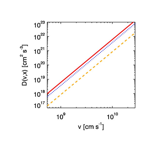
where [s] is the acceleration timescale, [cm] is the spatial extent of the acceleration region and is a constant that controls the strength of the velocity dependance. With this choice, we confine the acceleration to a region in space, akin to an extended looptop acceleration region, as observed by RHESSI (Xu et al., 2008; Kontar et al., 2011b; Guo et al., 2012, e.g.). Equation 6 assumes that the acceleration efficiency within this region is most effective at , the top of the loop, and that there is a drop off with distance that is Gaussian in nature. The length of the acceleration region, density and temperature are determined from RHESSI imaging spectroscopy and discussed in Section 3. The diffusion coefficient (Equation 6) is shown in Figure 1 for a specific choice of acceleration timescale, , spatial extent, , and thermal velocity, , the latter two obtained from imaging spectroscopy (see Section 3.2).
2.4 The leaky-box Fokker-Planck approximation
At this point it is instructive to examine the leaky-box Fokker-Planck approximation (Kulsrud & Pearce, 1969; Benz, 1977; Chen & Petrosian, 2013, e.g.). This model is a spatially averaged description of the velocity (or energy) evolution of electrons in the acceleration region designed to study the spectral properties of accelerated electrons, and has been used as a comparison to solar flares. Replacing transport by an escape timescale term we have the equation for the spatially-averaged distribution function, ,
| (7) |
where,
| (8) |
is the acceleration region averaged velocity diffusion coefficient and denotes spatial averaging over the full width half maximum (FWHM), . Equation (7) is informative and simple to use, but ignores the essential spatial dependencies in acceleration and transport. The stationary solution as can be readily obtained from the following equation,
| (9) |
Since the X-ray producing electron spectrum can often be approximated by a power-law (Holman et al., 2003), a stationary solution of Equation (9) in the form is assumed. Substituting this power-law solution of , we have,
| (10) |
Differentiating this expression and rearranging we can find an expression for , the power-law index. For scatter-free transport, the escape timescale is equal to the free streaming timescale, . Therefore, the spectral index is,
| (11) |
where one sees that a power-law electron spectrum ( independent ) can be obtained only for , so,
| (12) |
Of course, in order to put our results here, and those of the numerical simulations, in the context of the imaging spectroscopy results of Section 3 we need the index of the density weighted mean electron flux . Using the fact that in one-dimension this means that,
| (13) |
where the superscript makes clear this is the one-dimensional scatter-free expression and the subscript shows that this is the expected from the looptop.
Similarly, the three-dimensional Fokker-Planck (Equation 2) gives the power-law index,
| (14) |
where (Bian et al., 2014, e.g.) and is the mean free path of an electron due to pitch-angle scattering. For constant , the power-law again requires , so,
| (15) |
As before, but for the three-dimensional Fokker-Planck, , so we have,
| (16) |
where the superscript and subscript illustrates that this is the three-dimensional Fokker-Planck with diffusive transport for the looptop spectrum.
So, the above arguments give us the looptop spectral index predicted by the leaky-box Fokker-Planck solution, or , depending on whether there is negligible or strong pitch-angle scattering respectively. In order to find the footpoint spectrum predicted in both cases, one needs the electron escape rate from the looptop source, [e- s-1 per unit energy]. The number of particles per second per unit speed, [e- s-1 (cm s-1)-1], is the flux multiplied by the volume, that is,
| (17) |
Now, since for the one-dimensional Fokker-Planck the total number is this means that and so,
| (18) |
the total number for the three-dimensional case, however, is , so and,
| (19) |
The density weighted mean electron flux at the footpoint is given by,
| (20) |
and so for the one-dimensional case this gives,
| (21) |
which means,
| (22) |
A similar argument leads to,
| (23) |
for the three-dimensional case.
In both cases, the power-law spectral index depends on the value of . If there is point like acceleration at the apex of the loop, with this configuration, one might expect a spectral index close to or to form. However, the spatial non-uniformity of the acceleration region results in local acceleration times given by,
| (24) |
due to dependency of (equations 1 and 2) and hence a different local distribution function. Therefore, a spatially dependent acceleration region creates different spectral indices at each point in space. The resulting distribution function from the entire acceleration region is controlled by the transport between various spatial locations. The resulting spectral index (if a power-law is formed) could be different from that predicted by our leaky-box solution.
Table 1 shows the relationship between the spectral indices of the electron phase-space distribution, density weighted mean electron flux and photon spectrum. When comparing models in Section 4 we use the spectral indices of the density weighted mean electron flux, for the reasons discussed in Brown et al. (2003).
These results are compared to numerical simulations with non-spatially averaged acceleration and transport. The importance of including the spatial dependence is shown clearly in Sections 4.1 and 4.2.
| Symbol | Description | Spectral Index |
|---|---|---|
| electron speed distribution (one-dimensional) | ||
| electron velocity distribution (three-dimensional) | ||
| density weighted mean electron flux (one-dimensional) | (LT)
(FP) | |
| density weighted mean electron flux (three-dimensional) | (LT)
(FP) | |
| photon spectrum | (for electron-ion bremsstrahlung) |
3 RHESSI observations and properties of non-thermal electrons
We use observations from a well studied flare (24 Feb 2011 07:29:40 - 07:32:36 UT) to derive the properties of the acceleration region which are used as the input for our model simulations. This event was chosen due to it being on the limb, thus enabling easy selection of the looptop and footpoint sources. Further to this, the looptop source has enough high energy photons to adequately constrain the non-thermal population of electrons present there.
Using the CLEAN algorithm (Hurford et al., 2002) with a beam width parameter of (Simões & Kontar, 2013), the resulting image is shown in the top panel of Figure 3. The regions were chosen to have no overlap to avoid cross-contamination and the photon spectra obtained from the looptop and footpoint regions were forward-fit (Holman et al., 2003, see e.g.) with the vth and thin2 functions in OSPEX (Schwartz et al., 2002). The fits yield a density weighted mean electron flux, [e- cm-2 s-1 keV-1], suitable for comparison with either the thin- or thick- target model. While it may seem incongruous to fit the emission from the dense chromosphere with a function containing thin-target bremsstrahlung; in reality, since we are seeking to compare the observations to numerical results, it only matters that we assume the same bremsstrahlung cross-section in both cases. It does not matter which fit function you use for the non-thermal part of the photon spectrum, so long as you use the same for your numerical results. Brown et al. (2003) discuss the reasoning behind using as the natural middle ground when comparing observations to numerical simulations of the HXR spectrum.
For the non-thermal population of electrons the density weighted mean electron flux is (Simões & Kontar, 2013),
| (25) |
where [e- cm-2 s-1] is the normalisation flux obtained from the OSPEX fit, is the fitted power-law spectral index, and keV is kept constant for each fit. The thermal part of the spectrum provides the emission measure, [cm-3], and the temperature, [keV], in the coronal part of the loop, so that the density weighted mean electron flux (Brown & Emslie, 1988; Battaglia & Kontar, 2013) is,
| (26) |
3.1 Thermal and spatial source parameters

For estimating the cross-sectional area, and thus the volume of the thermal source, we assumed a loop like geometry joined to the chromosphere at the footpoints. The loop morphology of coronal sources has been extensively discussed in general, but not for this event, by Xu et al. (2008); Kontar et al. (2011b). Figure 2 shows a cartoon of the CLEAN image in the top panel of Figure 3 highlighting the pertinent measurements. The cross-sectional area is assumed to be circular, , with diameter, , being estimated by first identifying the maximum emission in the energy band, keV (as we are calculating the thermal volume to estimate the density from the emission measure, i.e. the thermal fit), then finding the distance bounded by the 50% contours and approximately orthogonal to the ‘loop midline.’ The thermal volume, , is then calculated by multiplying the area, , by the length of looptop emission, , which is obtained by approximating the length along the loop midline and again bounded by the contours, i.e. the FWHM of the thermal emission. The spatial extent of the acceleration region is assumed to be the standard deviation of the full width half maximum as in Xu et al. (2008) and is given by .
Using from thermal fit we obtained an estimate of the mean target proton density, assuming a Hydrogen plasma. The looptop source is best fit by an emission measure, cm-3, and a temperature, MK, seen in Figure 3 (lower left panel). We calculated cm-3 as described in the previous paragraph to obtain a looptop density, cm-3. The spatial extent of the acceleration region was calculated to be cm. These parameters are used as the input to our model corona.
3.2 Non-thermal spectral properties


The flux of non-thermal particles is cm-2 s-1 and the spectral index is . The footpoint sources, seen in the bottom middle panel in Figure 3, are best fit by a flux of cm-2 s-1 and a spectral index of . The imaging spectroscopy results are consistent with the full-Sun spectrum seen in the bottom right panel in Figure 3 ( cm-3, MK, cm-2 s-1 and ). The low energy cutoff was fixed at keV for all fits.
As expected the footpoint source has a harder spectrum of high energy electrons, but not by the factor two that would be expected if both coronal and footpoint photon spectra are fit with thin2 (Simões & Kontar, 2013, see). This implies some kind of extra trapping within the coronal looptop source (Simões & Kontar, 2013; Chen & Petrosian, 2013). Non-collisional pitch angle scattering in the presence of collisional losses hardens the electron spectrum in the coronal source at lower energies and this may result in both the looptop and footpoint spectra becoming broken power-laws (Bespalov et al., 1991). Fitting with a single power-law electron spectrum could thus result in spectral index differences between the looptop and footpoint sources that are not equal to two, as mentioned in Kontar et al. (2014). The spectra shown in Figure 3 show nothing in the residuals to suggest a break however, so it suffices to fit the non-thermal spectrum with a single power-law here.
4 Numerical solutions of the fokker-planck equation
We created a model corona with an originally Maxwellian distribution of particles at temperature, . This means that the thermal speed and,
| (27) |
The density, , is modelled as constant throughout the corona with an exponential increase at the chromosphere with scale height, km, following a hydrostatic model consistent with RHESSI observations (Battaglia & Kontar, 2012),
| (28) |
where is the end of the numerical box ( in this case) and is chosen to be sufficiently high to collisionally stop electrons. The density profile is shown in Figure 4. The spatial extent of the acceleration region, , calculated above was used in Equation (6). Setting for the reasons discussed in Section 2.4 we examined how the parameter affects the spectral index resulting from our simulations. The simulated index is compared to that predicted by the leaky-box solution (Equations 13, 16, 22 and 23) valid for each transport regime to see how the introduction of a spatially inhomogeneous, extended acceleration region affects the distribution of the energized particles. The timescales shown here are , where is the collisional timescale of a thermal electron in the corona, approximately s for the event in question ( is the coronal collisional parameter here, independent of ). These timescales are chosen as they result in the range of electron spectral indices typically found in solar flares. The Fokker-Planck equations were solved numerically by the method of finite differences (Kontar, 2001). The results are discussed in Sections 4.1 and 4.2, but first we discuss how to obtain , and specifically the power law index, , from the simulations to compare with the leaky-box solutions.

The electron phase space distribution, , used in our simulations is directly related to the observed mean flux spectrum, so that the electron flux spectrum is in the one-dimensional Fokker-Planck and for the three-dimensional Fokker-Planck. The density weighted mean electron flux is,
| (29) |
So we have,
| (30) |
where is the cross-sectional area of the loop and the limits are the estimation of the distance from the maximum emission in keV to one of the footpoints. The footpoint has a steeply increasing density (Figure 4) over the last 5 arcseconds of our simulation domain. The density weighted mean electron flux from the model footpoint is thus,
| (31) |
The power-law index of either the simulated looptop or footpoint source can then be found as,
| (32) |
where the dependence of is to make clear that the simulated will not be constant with due to the extended, spatially varying nature of the acceleration region. The simulated spectral index was fit with a power-law between 25 and 50 keV, the reason being that the spectral index of a solar flare may be expected to vary with energy as well, so fitting our simulated with a power-law enabled a fairer comparison. The spectral index for each will be compared to the equivalent leaky-box solution with differences highlighted. In the next two sub-sections we summarise the simulation results for the different transport regimes.
4.1 Scatter-free transport


Figure 5 shows the simulated density weighted mean electron flux, . This graph clearly illustrates the dependence of both the spectral index and non-thermal flux on the acceleration timescale, . The longer the acceleration timescale, the less efficient the particle acceleration and the steeper the spectrum.
The simulated spectral index from a power-law fit between 25 and 50 keV for each timescale studied is shown in Figure 6 and is compared to the leaky-box solution (Equations 13 and 22). The fitted spectral index for the 2011 Feb 24 flare is overplotted for context. At short times, , the spatially independent and inhomogeneous models agree for both the looptop and footpoint sources. However, there is a clear difference between the spatially independent leaky-box solution and the numerical solution to the Fokker-Planck (Equation 1) at times . For example, the fitted spectral index to the looptop is , the leaky-box Fokker-Planck predicts an acceleration timescale required to produce this spectral index of . That is to say this is the point where the blue diamonds overlap with the grey confidence band in Figure 6 (left-panel). The numerical solution of the spatially inhomogeneous model (Equation 1) predicts a softer index here and, as such, this model would require a shorter acceleration timescale, somewhere between to produce the observed looptop spectral index. This is particularly pertinent when one considers that typical looptop spectra are, in general, softer than that observed here, the typical range being (Battaglia & Benz, 2006, see e.g.). Therefore, in the range of ‘realistic’ spectral indices the spatially inhomogenous model produces softer spectra than the spatially independent model. Furthermore, the same behaviour is seen in the right panel of Figure 6 for the footpoint spectrum, where it is clear that for the observed the spatially independent model predicts a longer acceleration timescale than our spatially inhomogeneous model. It is also important to note that footpoint spectral indices are rare; in the right panel of Figure 6 it is easy to see that in the range there is a substantial difference between the acceleration timescales required by both models to produce the same spectral index.
In summary, the introduction of spatially inhomogeneous acceleration and transport reduces the acceleration efficiency compared to the spatially independent leaky-box formulation for the standard range of spectral indices observed by RHESSI. As a result, any acceleration timescale inferred from the the leaky-box approximation could be an overestimate of the actual acceleration timescale in the flare.
4.2 Diffusive transport with cm


Figure 7 shows the for diffusive transport with a constant mean free path of cm. This value is chosen due Kontar et al. (2014) finding it the midpoint of the limits for 30 keV electrons, as discussed earlier. Like Figure 5 we clearly see the relationship between the flux of non-thermal particles, the spectral index and the acceleration timescale.
The simulated spectral index is compared to that predicted from the leaky-box Fokker-Planck approximation (Equations 16 and 23) and the imaging spectroscopy results from the 2011 February 24 flare in Figure 8. We again see a similar behaviour to the scatter-free case for both the spatially independent and inhomogeneous models with respect to the acceleration timescale. For the realistic range of discussed in the previous section there is again a large difference between the index predicted by the leaky-box analytic solution and the spatially inhomogeneous model considered (Equation 2). Specifically, when spatial effects are fully taken into account the model produces a generally softer spectral index than the spatially independent leaky-box formalism. Thus, we again conclude that a timescale inferred when using the leaky-box model could in fact be an overestimation of the actual acceleration timescale in the system.
It is important to note that the (slightly) negative spectral indices obtained for the numerical simulations in Figures 6 and 8 arise from the shortest acceleration timescales studied (see grey and purple lines in Figures 5 and 7). Such spectral indices are not observed, however, and so the respective timescales are too short for the solar flare case.
5 Summary
In this paper we introduced a model accounting for the intrinsic spatial variation in the acceleration region of solar flares. By using the imaging spectroscopy of the 2011 February 24 flare the density, temperature and spatial extent of the acceleration region were inferred and used as input parameters to the model. We solved the governing kinetic equations numerically, and compared to the spatially invariant leaky-box approximation commonly used when studying stochastic acceleration in solar flares. The results are summarised as follows:
- •
Scatter-free transport; the introduction of a spatially inhomogeneous acceleration region while explicitly accounting for transport results in acceleration that is generally less efficient than the spatially independent leaky-box formulation. The resulting spectral index, for both looptop and footpoint sources, is softer than that when spatial effects are not explicitly taken into account.
- •
Diffusive transport with cm; similar behaviour is seen for the diffusive transport case, the introduction of a spatially extended, inhomogeneous, acceleration region results in a spectrum that is softer, for the most part, than that predicted by the leaky-box solution.
In summary, for both transport regimes studied it is clear that the intrinsic spatial dependency evident in solar flares (Xu et al., 2008; Guo et al., 2012) changes the resulting electron spectrum when compared to the spatially independent leaky-box approximation. It acts to reduce the acceleration efficiency and thus produces a softer spectrum. This is particularly pronounced in the ‘standard’ range of spectral indices, , generally observed by RHESSI ( and , see e.g. Battaglia & Benz, 2006). This means that the acceleration timescales inferred when using a leaky-box model applied to a solar flare could be an overestimation. These timescales should therefore be considered an upper limit of the time taken to produce the observed spectral index. Thus, the authors suggest that the intrinsic spatial dependence should be taken into account when modelling stochastic acceleration in solar flares.
Acknowledgements.
This work was supported by the STFC, via an STFC consolidated grant (EPK) and an STFC studentship (DJS). The work was undertaken at the University of Glasgow, and for that the authors express gratitude. DJS further wants to thank Researchers in Schools and King’s College London for honourary visiting researcher status, as well as the Co-op Academy Failsworth for allowing the continuation of research in a new career. Both authors would also like to thank the referee for their helpful comments to improve the paper.References
- Bai (1982) Bai, T. 1982, ApJ, 259, 341
- Battaglia & Benz (2006) Battaglia, M. & Benz, A. O. 2006, A&A, 456, 751
- Battaglia & Kontar (2012) Battaglia, M. & Kontar, E. P. 2012, ApJ, 760, 142
- Battaglia & Kontar (2013) Battaglia, M. & Kontar, E. P. 2013, ApJ, 779, 107
- Benz (1977) Benz, A. O. 1977, ApJ, 211, 270
- Benz & Smith (1987) Benz, A. O. & Smith, D. F. 1987, Sol. Phys., 107, 299
- Bespalov et al. (1991) Bespalov, P. A., Zaitsev, V. V., & Stepanov, A. V. 1991, ApJ, 374, 369
- Bian et al. (2012) Bian, N., Emslie, A. G., & Kontar, E. P. 2012, ApJ, 754, 103
- Bian et al. (2014) Bian, N. H., Emslie, A. G., Stackhouse, D. J., & Kontar, E. P. 2014, ApJ, 796, 142
- Brown & Emslie (1988) Brown, J. C. & Emslie, A. G. 1988, ApJ, 331, 554
- Brown et al. (2006) Brown, J. C., Emslie, A. G., Holman, G. D., et al. 2006, ApJ, 643, 523
- Brown et al. (2003) Brown, J. C., Emslie, A. G., & Kontar, E. P. 2003, ApJ, 595, L115
- Chen & Petrosian (2013) Chen, Q. & Petrosian, V. 2013, ApJ, 777, 33
- de Jager (1986) de Jager, C. 1986, Space Sci. Rev., 44, 43
- Dickson & Kontar (2013) Dickson, E. C. M. & Kontar, E. P. 2013, Sol. Phys., 284, 405
- Emslie (1983) Emslie, A. G. 1983, Sol. Phys., 86, 133
- Emslie et al. (2012) Emslie, A. G., Dennis, B. R., Shih, A. Y., et al. 2012, ApJ, 759, 71
- Emslie & Henoux (1995) Emslie, A. G. & Henoux, J.-C. 1995, ApJ, 446, 371
- Emslie et al. (2008) Emslie, A. G., Hurford, G. J., Kontar, E. P., et al. 2008, in American Institute of Physics Conference Series, Vol. 1039, American Institute of Physics Conference Series, ed. G. Li, Q. Hu, O. Verkhoglyadova, G. P. Zank, R. P. Lin, & J. Luhmann, 3–10
- Emslie et al. (2003) Emslie, A. G., Kontar, E. P., Krucker, S., & Lin, R. P. 2003, ApJ, 595, L107
- Fermi (1949) Fermi, E. 1949, Physical Review, 75, 1169
- Guo et al. (2012) Guo, J., Emslie, A. G., Kontar, E. P., et al. 2012, A&A, 543, A53
- Holman et al. (2011) Holman, G. D., Aschwanden, M. J., Aurass, H., et al. 2011, Space Sci. Rev., 159, 107
- Holman et al. (2003) Holman, G. D., Sui, L., Schwartz, R. A., & Emslie, A. G. 2003, ApJ, 595, L97
- Hurford et al. (2002) Hurford, G. J., Schmahl, E. J., Schwartz, R. A., et al. 2002, Sol. Phys., 210, 61
- Jeffrey & Kontar (2013) Jeffrey, N. L. S. & Kontar, E. P. 2013, ApJ, 766, 75
- Jeffrey et al. (2014) Jeffrey, N. L. S., Kontar, E. P., Bian, N. H., & Emslie, A. G. 2014, ApJ, 787, 86
- Johns & Lin (1992) Johns, C. M. & Lin, R. P. 1992, Sol. Phys., 137, 121
- Jokipii (1966) Jokipii, J. R. 1966, ApJ, 146, 480
- Kane et al. (1998) Kane, S. R., Hurley, K., McTiernan, J. M., et al. 1998, ApJ, 500, 1003
- Kontar (2001) Kontar, E. P. 2001, Computer Physics Communications, 138, 222
- Kontar et al. (2014) Kontar, E. P., Bian, N. H., Emslie, A. G., & Vilmer, N. 2014, ApJ, 780, 176
- Kontar & Brown (2006) Kontar, E. P. & Brown, J. C. 2006, ApJ, 653, L149
- Kontar et al. (2011a) Kontar, E. P., Brown, J. C., Emslie, A. G., et al. 2011a, Space Sci. Rev., 159, 301
- Kontar et al. (2011b) Kontar, E. P., Hannah, I. G., & Bian, N. H. 2011b, ApJ, 730, L22
- Kontar et al. (2004) Kontar, E. P., Piana, M., Massone, A. M., Emslie, A. G., & Brown, J. C. 2004, Sol. Phys., 225, 293
- Kulsrud & Pearce (1969) Kulsrud, R. & Pearce, W. P. 1969, ApJ, 156, 445
- Li & Gan (2005) Li, Y. P. & Gan, W. Q. 2005, ApJ, 629, L137
- Lin et al. (2002) Lin, R. P., Dennis, B. R., Hurford, G. J., et al. 2002, Sol. Phys., 210, 3
- Liu et al. (2009) Liu, R., Wang, H., & Alexander, D. 2009, ApJ, 696, 121
- McTiernan & Petrosian (1990) McTiernan, J. M. & Petrosian, V. 1990, ApJ, 359, 524
- Melrose (1968) Melrose, D. B. 1968, Ap&SS, 2, 171
- Peterson & Winckler (1959) Peterson, L. E. & Winckler, J. R. 1959, J. Geophys. Res., 64, 697
- Petrosian & Chen (2010) Petrosian, V. & Chen, Q. 2010, ApJ, 712, L131
- Petrosian & Donaghy (1999) Petrosian, V. & Donaghy, T. Q. 1999, ApJ, 527, 945
- Petrosian et al. (2002) Petrosian, V., Donaghy, T. Q., & McTiernan, J. M. 2002, ApJ, 569, 459
- Piana et al. (2003) Piana, M., Massone, A. M., Kontar, E. P., et al. 2003, ApJ, 595, L127
- Ryan & Lee (1991) Ryan, J. M. & Lee, M. A. 1991, ApJ, 368, 316
- Saint-Hilaire et al. (2008) Saint-Hilaire, P., Krucker, S., & Lin, R. P. 2008, Sol. Phys., 250, 53
- Schwartz et al. (2002) Schwartz, R. A., Csillaghy, A., Tolbert, A. K., et al. 2002, Sol. Phys., 210, 165
- Simões & Kontar (2013) Simões, P. J. A. & Kontar, E. P. 2013, A&A, 551, A135
- Sturrock (1966) Sturrock, P. A. 1966, Physical Review, 141, 186
- Tandberg-Hanssen & Emslie (1988) Tandberg-Hanssen, E. & Emslie, A. G. 1988, The physics of solar flares (Cambridge and New York, Cambridge University Press)
- Veronig & Brown (2004) Veronig, A. M. & Brown, J. C. 2004, ApJ, 603, L117
- Xu et al. (2008) Xu, Y., Emslie, A. G., & Hurford, G. J. 2008, ApJ, 673, 576