Hyperspectral recovery from RGB images using Gaussian Processes
Abstract
We propose to recover spectral details from RGB images of known spectral quantization by modeling natural spectra under Gaussian Processes and combining them with the RGB images. Our technique exploits Process Kernels to model the relative smoothness of reflectance spectra, and encourages non-negativity in the resulting signals for better estimation of the reflectance values. The Gaussian Processes are inferred in sets using clusters of spatio-spectrally correlated hyperspectral training patches. Each set is transformed to match the spectral quantization of the test RGB image. We extract overlapping patches from the RGB image and match them to the hyperspectral training patches by spectrally transforming the latter. The RGB patches are encoded over the transformed Gaussian Processes related to those hyperspectral patches and the resulting image is constructed by combining the codes with the original Processes. Our approach infers the desired Gaussian Processes under a fully Bayesian model inspired by Beta-Bernoulli Process, for which we also present the inference procedure. A thorough evaluation using three hyperspectral datasets demonstrates the effective extraction of spectral details from RGB images by the proposed technique.
Index Terms:
Hyperspectral imaging, Spectral recovery, Gaussian Process.I Introduction
Hyperspectral images preserve the fine spectral details that are lost in RGB images due to the gross quantization of scene radiance. These details are desirable in numerous imaging applications, ranging from Remote Sensing to Medical Imaging and Forensics [2], [12], [17], [19], [33], [37], [68]. More recently, spectral characteristics of signals have also been shown to improve performance in multiple Computer Vision tasks, such as recognition [60], [61], [66]; tracking [35], [43]; pedestrian detection [29] and document analysis [34]. This fact has motivated a wider interest of Computer Vision community in hyperspectral imaging [3], [4], [7], [16], [36], [56].
Hyperspectral cameras integrate scene radiance under dozens (or even hundreds) of spectrally well-localized basis functions. This results in images with a large number of spectral channels, each capturing the scene reflectance in a precise wavelength range. However, to maintain an acceptable signal-to-noise-ratio of each spectral channel, hyperspectral cameras generally require longer exposure time. Moreover, as compared to their color counterparts, present-day hyperspectral cameras severely lack in terms of spatial resolution [4], [36]. This problem stems directly from the fact that increasing the sensor resolution in hyperspectral cameras further reduces the photon density at the sensor, which is already limited by the narrow wavelength intervals of the spectral channels. Owing to the specialized hardware that accounts for these issues, current off-the-shelf hyperspectral cameras are expensive and their use is largely limited to the applications where the temporal and spatial resolution of imaging is not critical.
Hyperspectral imaging using computational techniques [7], [24], [44], [54] is an affordable alternate to exploit the power of spectral domain in more common imaging applications, which makes it an interesting research problem. Goel et al. [24] proposed to estimate up to 17 distinct spectral channels for scenes by augmenting a regular color camera with a time-multiplexed illumination source. Oh et al. [44] used the disparity between the spectral responses of multiple color cameras to compute scene reflectance at the wavelengths other than those of camera spectral channels. Similarly, Takatani et al. [56] augmented a conventional camera with a tube of faced reflectors and estimated the scene spectra beyond the sampling wavelengths of camera channels. Arad and Ben-Shahar [7] also demonstrated recovery of higher dimensional spectra from three channel color images. They factorized the color image and a set of training hyperspectral images into their corresponding bases and coefficient matrices. Later, the coefficient matrix of the color image is used with the hyperspectral basis to construct a hyperspectral image.
The technique proposed by Arad and Ben-Shahar[7] is unique in the sense that it does not require any external hardware/illumination source besides a single conventional camera. Inspired by the paramagnetic nature of this paradigm, we also propose to recover spectral details from a single RGB camera. However, in contrast to [7], we mainly focus on the physical attributes of reflectance spectra for their accurate recovery. It is a common knowledge that naturally occurring reflectance spectra are relatively smooth functions of wavelength [8]. Gaussian Processes [52] can explicitly model such smoothness using Kernels, which makes them an ideal tool for spectral recovery. Similarly, self-similarity of spatial patterns and spectral sources within a scene [16], and non-negativity of reflectance are other physical attributes that we exploit to construct hyperspectral signatures from RGB images.

Concretely, we propose to learn multiple sets of Gaussian Processes from training hyperspectral image patches. For the overall approach, an element (i.e. a Gaussian Process) in a given set signifies a distribution over a spectral source in the training data. We can expect hyperspectral image regions containing similar materials/spectral-sources to be spatio-spectrally similar. Therefore, we use clusters of spatio-spectrally correlated patches to learn their corresponding sets (see Fig. 1). We transform the Mean parameters of the inferred Gaussian Processes to match the spectral quantization of the RGB image. The transformed Means are used to encode overlapping patches of the RGB image. To ensure effective coding, we first match an RGB patch to the RGB transformations of the hyperspectral training patches, and use the Means corresponding to the right cluster. The codes of RGB patches are combined with the original Gaussian Processes to estimate the detailed spectra of the scene.
We propose to learn the desired Gaussian Processes under a representation model inspired by Beta-Bernoulli Process [46]. However, instead of using simple multi-variate Gaussian distributions in the model [46], we employ Gaussian Processes as the base measure with appropriate Kernels for spectral modeling. We additionally place Gamma hyper-prior over the Kernel parameter for its automatic adjustment to the training data. Moreover, we also encourage non-negativity in the inferred signals for modeling the reflectance values. Our Bayesian representation model is fully conjugate, which allows us to analytically derive the posterior distribution expressions for inferring the desired Gaussian Processes. We use Gibbs sampling as the inference technique and provide its sampling equations. The approach is thoroughly evaluated by recovering the hyperspectral images from RGB images of more than 35 Indoor, Outdoor and Object scenes from three different hyperspectral databases - CAVE database [64], iCVL database [7] and the Harvard dataset [11]. Experimental results demonstrate the effectiveness of the proposed approach, achieving up to reduction in the RMSE value for the spectral recovery as compared to [7].
The article is organized as follows. In Section II, we review the literature related to the proposed approach. The underlying problem is formalized in Section III and the possibility of recovering spectral details from RGB signals is analyzed in the light of the existing literature in Section IV. In Section V, we present the proposed approach, whereas its implementation details are discussed in Section VI. Experimental evaluation is presented in Section VII, and the article concludes in Section VIII. We also provide the details on the joint probability distribution of the proposed model and the derivations of Gibbs sampling equations for our approach in Appendices (supplementary material).
II Related Work
Hyperspectral imaging systems have been in use in Remote Sensing platforms for nearly three decades [55]. Early hyperspectral systems such as NASA’s AVIRIS [25] acquired images using the ‘whisk broom’ scanning method that uses a set of mirrors and fiber optics to re-direct the incoming light to a bank of spectrometers. More recent systems use the ‘push broom’ scanning strategy [31] that employs dispersive optical elements and light sensitive sensors to obtain a hyperspectral image in a line-by-line manner. For the on-ground applications, hyperspectral images are commonly acquired with the help of interchangeable or tunable narrow band filters [42], [58]. However, with the exception of a few, e.g. coded aperture snapshot spectral imager [70]; most of the specialized hardware based strategies fall short of performing hyperspectral imaging with the spatial and temporal resolution that is generally required in the common Computer Vision tasks. This fact has led to a considerable recent interest of researchers in the computational methods for hyperspectral imaging.
To construct the 3D hyperspectral data cube, Computed Tomography Imaging Spectrometers project the spatio-spectral signals on to 2D sensors using diffraction grating, and computationally estimate hyperspectral images from these projections [15], [32], [45]. Whereas effective hyperspectral cubes can be constructed with this technique, the methods require both specialized hardware as well as considerable post-processing to achieve these results. Furthermore, the spatial resolution of the resulting cube is again limited by the used sensor. Brady and Gehm [10], and later Gehm et al. [23] used the techniques from compressive sensing to improve on the sensor limitations. Nevertheless, the specialized image acquisition setup and the significant post-processing remains the bottleneck in the widespread use of the Computed Tomography Imaging Spectrometers for hyperspectral imaging.
Hyperspectral fovea systems [21], [62] have also been proposed with an aim to acquire real-time hyperspectral images with less complex post-processing. These systems capture a high resolution color image along the spectral information of the central region in the image. Although useful, these systems are more suitable for the applications where occasional hyperspectral sampling of specific regions is required instead of obtaining the spectral details of the whole area [7]. Another direction of computational techniques related to the high resolution hyperspectral imaging [3], [6], [33], [36] uses matrix factorization to compute a spectral basis from a low resolution hyperspectral image and uses it to augment the spectral dimension of the color image of the same scene. Whereas these methods have to shown impressive reconstruction of hyperspectral cubes, the assumption of availability of the low resolution hyperspectral image can only be satisfied by the specialized hyperspectral hardware.
A number of computational methods for extracting the spectral information of the scene using color imaging also rely on active scene illumination. For instance, D’Zmura [18] estimated the reflectance of the scene with the help of illumination patterns with independent spectral characteristics. Their approach recovers the scene reflectance by finally estimating the coefficients of a linear representation model. In a similar approach, Park et al. [48] reconstructed hyperspectral frames of a video using a multiplexed illumination setup that combines different color LEDs to illuminate the scene. Chi et al [13] estimated the spectral reflectance of the scene by placing a set of wide band filters in front of the light source. A DLP projector along a high-speed camera was used by Han et al. [27] to recover the scene reflectance. Moreover, a time multiplexed illumination was also employed by Goel et al. [24] to estimate the scene reflectance across 17 spectral channels at 9 frames per second. Parmer et al. [50] showed successful estimation of 31 spectral channels with the help of five time-multiplexed LED sources. The method images the same scene multiple times to compute the target 31 spectral channels.
Methods for scene reflectance estimation inspired by kaleidoscope geometry also appear in the literature. For instance, Han and Perlin [26] used a tapered kaleidoscope to estimate the bi-directional texture reflectance of a surface. Manakov et al. [41] proposed a reconfigurable camera ad-on based on the principle of kaleidoscope for a high dynamic range multi-spectral and light field imaging. A similar approach has been adopted by Takatani et al. [56] who used faced color filters in a kaleidoscopic configuration for multiple reflections of the incoming light to the sensor. The different spectra resulting from different reflections are exploited in their approach to computationally estimate the scene reflectance at wavelengths other than the central wavelengths of the spectral sensitivity of the camera.
Along the lines of the technique proposed in this work, there have been previous attempts to directly recover spectral details of scenes using RGB cameras. For instance, Nguyen et al. [71] leveraged RGB white-balancing for scene illumination normalization, and recovered the scene reflectance using color images and a radial basis function network trained on hyperspectral data. Robles-Kelly [72] extracted spectral and convolutional features from training hyperspectral data by employing sparse coding and used those features to construct hyperspectral images from RGB images. Whereas material properties are considered in [72], the method does not take any advantage of the intrinsic properties of natural spectra. A closely related method to our approach is proposed by Arad and Ben-Shahar [7], that learns a hyperspectral basis from training data and transforms it to sparsely encode RGB images. The RGB sparse codes are then combined with the original basis for the spectral recovery of scene reflectance.
The technique of Arad and Ben-Shahar closely relates to our previous work [3], except that it uses a corpus of separately acquired training data instead of a low resolution hyperspectral image of the scene to learn the hyperspectral basis. This eliminates the need of hyperspectral hardware during the testing phase. Galliani et al. [54] exploited hyperspectral training data in the context of deep neural networks [75] to learn a mapping from three to multiple spectral channels. Later, Wu et al. [74] argued in favor of hyperspectral reconstruction using shallow methods, e.g. [7] as opposed to the deep networks employed by Galliani et al. [54]. Based on a method exploiting adjusted anchored neighborhood regression for super-resolution [76], Wu et al. [74] also proposed an improvement over [7]. Another approach that exploits neural networks for spectral recovery is proposed by Alvarez-Gila et al. [73] that uses Generative Adversarial Networks [77] to learn a mapping from three to multiple spectral channels.
Whereas the above methods relate to the proposed approach, our technique particularly emphasizes on exploiting the intrinsic attributes of spectral signatures for hyperspectral recovery in a principled manner - in which the existing approaches fall considerably short. It is noteworthy that currently there is a growing interest in the research community for the problem of hyperspectral recovery from RGB images. Very recently, the first on-line challenge on spectral reconstruction from RGB images has also been introduced at the NTIRE workshop (http://www.vision.ee.ethz.ch/ntire18/) conducted in conjunction with CVPR 2018. The challenge required spectral recovery from RGB images constructed by applying known and unknown spectral response functions to the ground truth hyperspectral images. Considering the interest of research community, a principled approach for spectral recovery from RGB images is expected to appropriately guide this emerging direction.
III Problem formulation
We denote an RGB image by , where spectral channels. From , we aim to construct a hyperspectral image of the same scene, where . From one perspective, our objective is to computationally improve the spectral resolution of an RGB image. In this work, we limit this improvement to by letting . For all practical purposes, we can assume a mapping function such that . This function integrates the spectral channels of the desired hyperspectral image to form the RGB image.
Let denote a pixel of the hyperspectral image. Due to multiple scatterings of light and presence of intimate material mixtures in a scene, this pixel is often formed as a combination of the spectral signatures of various materials in the scene. Considering all the distinct spectral signatures of the scene materials to be present in a matrix , we may represent a hyperspectral image pixel as , where is the coefficient vector in . This representation model is commonly employed in hyperspectral unmixing [5], [8]. Due to the existence of the mapping function , we can further represent the corresponding pixel of the RGB image as , where is the spectral transformation between the target hyperspectral image and the acquired RGB image. In this work, we consider this transformation matrix to be known a priori. We note that prior knowledge of is a common assumption in the image fusion based hyperspectral super-resolution literature [3], [33], [36] and it can be estimated using the spectral response of the cameras.
From the above, we can see that with the help of correctly computed signatures in one can hope to recover a much more detailed spectral response of the scene at image pixel level. Assuming a hyperspectral training prior, we aim to estimate the desired signatures using Gaussian Processes that account for the physical attributes of natural spectral, such as their relative smoothness and non-negativity of reflectance values.
IV Spectral recovery from RGB signals
On the surface, the attempt to recover -dimensional signatures from three dimensional RGB signals may appear over ambitious. Arguably, the problem is severely under-constrained because the spectral quantization process of the RGB cameras suffers from the phenomenon of metamerism [47] - perceived/sensed matching of the colors that do not actually match based on the differences in their spectral power distribution. This means, multiple spectral signatures (metamers) can exist for a given RGB pixel. Thus, it is interesting to ask that to what extent hyperspectral signals can really be recovered from the RGB signals?
Arad and Ben-Shahar [7] strongly argued that under certain conditions the detailed spectral information from RGB signals is indeed recoverable. The conditions they stipulate for that purpose are as follows. (1) It is required that the set of spectral signals encountered by the sensor is actually confined to a relatively lower dimensional manifold within the high dimensional space of the possible hyperspectral signals, and (2) the frequency of the metamers in that lower dimensional manifold is low. If these conditions hold, the RGB signals may be able to reveal much finer spectral details of the scene than what has been recorded by the sensor.
Existing studies [69], [40], [49] have consistently shown that the reflectance spectra of materials are generally well represented by a small number of principal components. Parkinnen et al. [49] demonstrated that only eight characteristic spectra are needed to achieve a good representation of 1,257 reflectance spectra of the chips in the Munsell Book of Color - Matte Finish Collection [69]. Haderberg [28] computed the effective dimension of the reflectance signatures of a large variety of color pigments to be between 13 to 23. More recently, Chakrabarti and Zickler [11] also showed that the first 20 principle components of their sampled hyperspectral image patches of more than seventy Indoor and Outdoor scenes were able to account for sample variance. Thus, a strong evidence already exists in favor of the above mentioned condition (1). In regards to condition (2), computing the relative frequency of the metameric pairs, Foster et al. [22] found that this value is usually as low as to for the natural scenes. From the perspective of recovering spectral details from RGB images, it indicates a high probability of recovering the correct metamer from the sensed signal. Hence, correct recovery of a hyperspectral image from its RGB counterpart indeed seems possible. Nevertheless, availability of a useful prior over the hyperspectral image is imperative.
In this work, we make the practical assumption that this prior is available in the form of hyperspectral image training data. Although hyperspectral cameras are currently not as popular as their RGB counterparts, public hyperspectral image databases have started emerging in the recent years. For instance, Arad and Ben-Shahar [7] collected one hundred hyperspectral images of urban, rular, indoor and plant-life scenes with a Specim PS Kappa DX4 camera. Chakrabarti and Zickler [11] made public 50 Outdoor and 27 Indoor scene hyperspectral images. The hyperspectral imaging laboratory at the University of Western Australia has also made hyperspectral image databases for Human Faces [61] and Documents [34] publicly available. Another example of a well-known public database of hyperspectral images of daily life objects is the CAVE database [64].
V Proposed approach
Our approach recovers the spectral details from RGB images by inferring multiple sets of Gaussian Processes using relevant hyperspectral training data and meticulously combining them with the RGB images. We exploit the Kernels of Gaussian Processes to model the relative smoothness [8], [63] of naturally occurring spectra. Moreover, the approach also accounts for the non-negativity of reflectance values and the self-similarity of hyperspectral image patches [16] for accurate spectral recovery. The schematics of the proposed approach is illustrated in Fig. 1. The overall approach can be divided into training and testing phases. We provide details on each of these phases below.
V-A Training
At the heart of the training phase is learning of Gaussian Processes () that represent hyperspectral signatures under a Bayesian model. For clarity, we defer the details on the proposed model and its inference scheme to the Sections to follow, and first summarize the remainder of the training phase. To learn the Gaussian Processes, the approach pre-processes the training hyperspectral data by extracting -dimensional patches from the images and arranging them in ‘’ clusters using K-Means algorithm. Processing hyperspectral images in terms of clustered patches is advantageous for our approach for two main reasons. Firstly, due to their similarity, the signals in each cluster are likely confined to an even lower dimensional manifold within the signal space. Secondly, within each cluster the frequency of the metamers [47] is naturally reduced because the clusters are generally composed of the same/similar spectral sources (e.g. patches corresponding to ‘grass’ cluster well together). From Section IV, we know that these properties of spectral signatures are conducive for the accurate recovery of the spectral details from RGB images, which benefits the overall approach.
We infer a set of ‘’ Gaussian Processes to represent the cluster of the training data. According to our model, the Gaussian Processes signify the spectral signal sources in the training data. Hence, we embed the smoothness of spectral signatures into these Processes using their Kernels. Moreover, we also use positive Mean priors in our model to incorporate non-negativity of reflectance values and the proportions in which the spectral signals generally mix to form image pixels [17]. With the help of the Bayesian inference (see Section V-A2) over the proposed model we learn posterior distributions for the Gaussian Processes. The Mean parameters of the learned distributions are then transformed to match the spectral quantization of the RGB camera11 1 The Kernels are not transformed because they are not required in the subsequent processing of the data.. Fig. 1 shows the transformed parameters for the cluster as a matrix , where is the transformed Mean of the Gaussian Process for the cluster. This matrix is later used in the testing phase of the approach.
V-A1 Representation Model
To infer the Gaussian Processes we propose to represent the hyperspectral pixel as follows:
| (1) | ||||
In the above model, denotes the matrix composed of a set of (possibly over-complete) basis vectors to represent the hyperspectral signatures. The vector models the Gaussian noise and is the coefficient vector for the representation. We place a separate Gaussian Process prior over each of the basis vectors, with the Mean and the Kernel . In Eq. (1) and the text to follow, we use the subscript ‘’ to distinguish the parameters of the prior probability distributions. Based on the analogy between the Beta-Bernoulli Process [46] underlying our model and the Dictionary Learning paradigm [59], we compute using the Online Dictionary Learning method proposed by Mairal et al. [38]. We provide details on this computation in Section V-A3. To promote the spectral correlation between the two consecutive channels of the hyperspectral signals at wavelengths and (in nano-meters), we used an exponential Kernel for the Gaussian Processes. For the Kernel, the parameter ‘’ loosely corresponds to the number of the consecutive spectral channels of that the Kernel is able to influence through extrapolation. The value determines the average distance of the underlying function from the Mean, which makes the ‘precision’ of the Kernel. Therefore, we let the training data itself determine the value of for the proposed model by placing a non-informative Gamma hyper-prior over this parameter. In Eq. (1), this is denoted by the Gamma distribution Gam(.) with parameters and . The parameters in the argument of the exponential function mainly depend on the hardware specifications of the hyperspectral sensor. Therefore, no further hyper-priors are placed over these parameters.
Following the formulation of the weighted Beta-Bernoulli Process [46], we model the coefficient vector as the Hadamard product of a binary vector and a Gaussian vector . The coefficient of is drawn from a Bernoulli distribution Bern(.) with the parameter . Moreover, a conjugate Beta prior, i.e. Beta(.) is placed over with the hyper-parameters and a scaling factor . The coefficients of are sampled from a Gaussian distribution with the mean and the precision . Notice that, in this formulation the basis vectors are associated with the signals under Bernoulli distributions that govern the support (i.e. ) of the coefficient vectors. Zhou et al. [67] noted that in Beta-Bernoulli formulation, the Bernoulli parameters automatically adjust to account for the intrinsic sparsity of the signals during the Bayesian inference, thereby generally rendering the coefficient vectors , to become sparse. Taking advantage of this observation, we estimate the Mean parameters of the prior distributions over by computing sparse representations [57] of the training signals over the Mean parameters of the Gaussian Process priors. The details on this computation are also provided in Section V-A3. We further place a non-informative Gamma hyper-priors over the precision of to automatically tune the value of this parameter to the training data.
The model assumes white noise with precision that is sampled from a Gamma distribution with the hyper-parameters and . We note that the proposed model significantly differs from the original proposal of the Beta-Bernoulli Process [46] in that (1) it uses Gaussian Processes with explicit Kernels instead of using the standard multivariate Gaussian distributions and (2) it uses non-zero Mean priors over the basis vectors as well as the coefficient vectors to promote non-negativity in the representation. We provide the analytical expression for the joint probability distribution over the training data defined by the proposed model in the Appendix A (supplementary material).
V-A2 Bayesian Inference
Our approach uses model (1) to learn posterior distributions over its parameters for hyperspectral data representation. We use Gibbs sampling technique [9] to infer those distributions. Being fully conjugate, the model allows us to derive analytical expressions for the posterior distributions. The inference process uses those expressions to iteratively draw samples from the respective probability distributions, and converge to the final posterior distributions. Below, we provide the analytical expressions used by our Gibbs sampler. The sampler sequentially draws samples from each of these distributions and keeps iterating until convergence. To avoid cluttering, we only provide the final expressions of the distributions below. The details of arriving at these expressions are separately given in Appendix B.
In the equations below, denotes the -norm of a vector and is the contribution of the basis vector in representing . That is,
.
For brevity, we also let .
Sample : from , where
Sample : from Gam, where
Sample : from , where
Sample : from , where
Sample : from , where
Sample : from , where
Sample : from , where
V-A3 Prior distribution parameter computation
The Gibbs sampling process estimates the posterior distributions for our model parameters. However, to start sampling, we require pre-computed Means and of the prior distributions over the basis vectors and the weights of the representation coefficients. Note that, the values of the ‘precision’ of the prior distributions is not important in our approach because of the used non-informative Gamma hyper-priors. However, the values of the Mean parameters of the prior distributions directly affect the posterior distributions. We exploit this fact to encourage non-negativity in the posterior distributions over and by restricting the Mean parameters of the prior distributions over these parameters to be strictly non-negative values, computed by solving the following constrained sparse optimization problem:
| (2) |
where and are the Frobenius and norms respectively, comprises the hyperspectral pixels (i.e. spectra) arranged as its columns, and denote the and the columns of and respectively, and is a pre-defined constant.
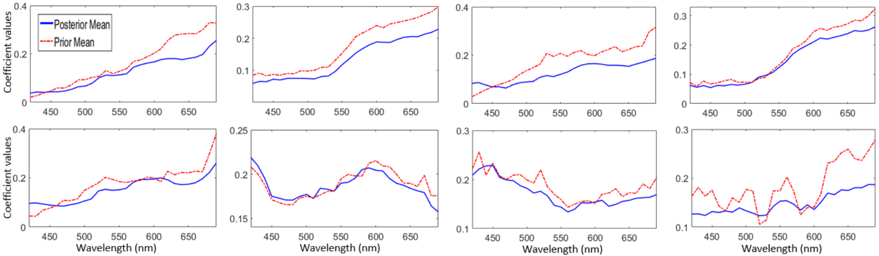
We use the columns of computed in Eq. (2) as in our approach whereas the coefficients of are used as the values of . Notice that, the coefficient matrix is constrained to be sparse. Furthermore, is allowed to be an over-complete dictionary for the training data. These properties are in-line with our representation model (1). Therefore, the factorization of the training data under Eq. (2) serves well for computing the prior distribution parameters for the proposed model. It is worth mentioning that the computed prior distribution Means only provide an informed guess for the posterior distributions in our model. The Means of the posterior distributions estimated by our approach are generally significantly different from the values computed by solving (2). To illustrate, Fig. 2 plots eight representative prior Means and their corresponding posterior values computed by the proposed approach (for CAVE database [64]). Details of the experiment are provided in Section VII. From the top-left to bottom-right of the figure, the columns of (i.e. Prior Means) are arranged in descending order of their usage in data factorization under Eq. (2). Along a visible difference between the prior and the corresponding posterior values, we can also observe that the posterior Means are smoother function of wavelength in the figure. This is true even for the cases where the prior spectra are already relatively smooth functions of wavelength. Note that, the smoother spectra in generally correspond to the lower frequency components in our data factorization. Another important observation in the figure is that the posterior Means are completely confined to the non-negative values.
V-B Testing
As indicated in Fig. 1, the testing phase uses the spectrally transformed (posterior) Means of the Gaussian Processes to represent the (-dimensional) patches of the test RGB image. The transformed Means are stored in ‘’ matrices . To choose an appropriate to represent a given RGB patch, the latter is first assigned a cluster of similar RGB patches by computing its Euclidean distances from the cluster centroids. These clusters are directly computed by spectrally transforming the already clustered hyperspectral patches, under the same transformation that is applied to the Mean parameters of the Gaussian Processes. The transformation of the clustered hyperspectral patches is an off-line process in our approach and it is performed only once for a given training dataset.
Once the RGB patch is assigned its cluster, the corresponding is used to represent the patch by solving the following optimization problem for each pixel :
| (3) |
where is a pre-defined constant. The target hyperspectral pixel is computed by taking the linear combination of the Gaussian Process Means in weighted by the coefficients of . In Eq. (3), we constrain to be sparse by restricting its -norm, which is to match the underlying sparisty of the spectral signals captured by our representation model with the Beta-Bernoulli distributions. Our approach extracts overlapping patches from the RGB image and performs the above mentioned process for each patch. A pixel in the estimated hyperspectral image is computed as the Expected value of the reconstructed spectra for that pixel.
VI Implementation details
We implement our approach using Matlab, running on an Intel Core i7 CPU at 3.6 GHz with 32 GB RAM. To solve the optimization problems (2) and (3), we used the SPAMS library [39] that implements the Online Dictionary Learning method [38] to solve (2) and the non-negative variant of the LARS algorithm [20] to solve (3). The values of the parameters and for these problems are empirically chose to be 0.01 and , respectively. It is worth mentioning that the precise value of is relatively unimportant for our approach as it only influences the prior parameters, for which posterior values are again computed. However, a small value of is preferable for our method that aims to compute an accurate mapping of a given RGB image to a hyperspectral image. We note that the SNR of RGB image can influence this parameter value. A low SNR of RGB image should be accounted for in Eq. (3) by choosing a larger reconstruction error . The value chosen in our experiments results in the best performance under the used evaluation protocol.
For our Bayesian model (1), we chose the values of the parameters based on the parameter significance. Except and , the parameters to belong to the non-informative Gamma hyper-priors in our model. Therefore, the inferred posterior distributions largely remain insensitive to their small values, e.g. in the range . This fact is easily verifiable from the sampling expressions in Section V-A2. We chose as the value for these parameters. Following [4], we used the same values for and , i.e. . For the Beta distributions, we set the value of equal to the number of Gaussian Processes to be learned, i.e. , whereas itself is automatically decided by the cluster size. The ratio of to the total number of Gaussian Processes to be learned for the complete training data is kept the same as the ratio of the number of patches in the cluster to the total number of training patches.
Based on the fact that our training data is largely clean in terms of Gaussian noise, we set the precision of the noise . Similarly, was also set to the same value because we set the initial values of equal to the computed , implying that we believe to be already a reasonable estimate of the posterior distribution over . The parameters were simply initialized to the support of . We also initialized with the values of the prior Mean parameters of the Gaussian Processes. All the Bernoulli parameters were initialized to the non-informative value . For the Gaussian Process Kernels, we chose as of the total number of channels in the resulting hyperspectral image.
Note that, due to the Bayesian nature of our approach, meaningful interpretations can be associated with most of the model parameters. We used these interpretations to guide us in choosing the initial values of the parameters. Nevertheless, we also tested the approach with multiple other close-by initial parameter values and found that the results remain fairly robust to those different initializations, which is typical for a Bayesian approach.
VII Experimental evaluation
We evaluated the proposed approach using the hyperspectral images from CAVE database [64], iCVL database [7] and Harvard database [11]. To benchmark, the approach is compared with the related technique of hyperspectral recovery from the RGB images proposed by Arad and Ben-Shahar [7], and Aeschbacher et al. [74], i.e. A+. We carefully implemented [7] (public code is not available) using the SPAMS library [39] and the efficient implementation of the K-SVD algorithm [1] provided by Rubinstein et al. [53], and used the author provided code for A+ [74]. In the original work [7], the authors proposed to use the Orthogonal Matching Pursuit (OMP) algorithm [51] to perform sparse coding of the test pixels over a known dictionary. Our experiments showed that sparse coding using the LARS algorithm [20] instead, consistently improves the accuracy of their method22 2 This observation is also well supported by the existing literature [5], [30]. The greedy pursuit strategy of OMP is more susceptible to the commonly found high mutual coherence of the spectral dictionaries as compared to the LARS algorithm [20].. Therefore, we performed the sparse coding by solving (3) in our implementation. This also allowed for a more fair comparison as we are able to use the same value of (i.e. ) for [7] and our approach. For the CAVE and the iCVL databases we also provide the results of employing our framework in a non-Bayesian settings. That is, instead of computing the Gaussian Processes, we directly use the bases computed by the Online Dictionary Learning method [38] in-place of the Gaussian Process Mean parameters in our framework. We denote this variant of our technique as ‘DL’ (for Dictionary Learning). The approach in [7] is mentioned as ‘Arad’ (after the author’s name). For each experiment, the total number of the Gaussian Processes in our approach are kept exactly the same as the total number of the dictionary atoms used for the other approaches, i.e. for the CAVE and Harvard images and for the iCVL images. These parameters were optimized for [7] using the cross validation technique and the values were directly used for the other approaches. In all the experiments, we fixed the number of clusters ‘’ to 10, and used spatial patches.
In our experiments, we treated the hyperspectral image from a database as the ground truth and transformed it to the RGB image using the spectral response of the Nikon D700 camera. We adopt this protocol from the RGB+hyperspectral image fusion literature [3], [33], [36]. We used the Root Mean Square Error (RMSE) and the Spectral Angle Mapper (SAM) [65] as the evaluation metrics. Whereas RMSE is useful in analyzing the reconstruction of the individual spectral channels of the estimated hyperspectral image, SAM provides a better assessment of the image reconstruction along the spectral dimension. The SAM value indicates the angle between the computed and the ground truth spectra (in degrees) - a lower value is more desirable. In the case of iCVL database, many images contain a large contrast in the scene illumination due to the presence of shadows in the images. Therefore, to avoid bias in the RMSE values we used the relative RMSE for iCVL images, computed by normalizing the error with the ground truth.
VII-A CAVE images
The CAVE database [64] consists of hyperspectral images of 32 daily life object scenes, acquired by the cooled CCD camera Apogee Alta U260 in conjunction with the Varispec liquid crystal tunable filter under the CIE standard illuminant D65. The -dimensional hyperspectral images are collected in the wavelength range 400nm - 700nm, with 10nm steps. The imaged scenes contain a variety of objects with distinct spectral responses, which makes the hyperspectral recovery for the CAVE images particularly challenging. Due to low signal-to-noise ratio and blur, we removed the first two and the last spectral channels of the hyperspectral images of this dataset in our experiments. We also do the same for the iCLV and the Harvard images in the Sections to follow.

For evaluation, we randomly selected seven different scenes from the CAVE dataset for testing. The RGB images of the testing scenes are shown in Fig. 3. The variety of the spectral sources is easily noticeable in the chosen scenes by considering the different colors present in the images. To learn the Gaussian Processes, we randomly selected five different hyperspectral images from the database for each test scene, ensuring that the test scene is not present among those images. The same training images are used for all approaches in our experiments. Table I summarizes the results of experiments, with best results bold-faced.
| Images | RMSE | SAM | ||||||||
|---|---|---|---|---|---|---|---|---|---|---|
| Prop. | DL | Arad [7] | A+ [74] | Prop. | DL | Arad [7] | A+ [74] | |||
| Feathers | 7.89 | 8.11 | 9.17 | 8.56 | 12.02 | 13.71 | 15.06 | 13.09 | ||
| Peppers | 5.74 | 7.18 | 7.64 | 6.99 | 16.34 | 17.76 | 18.45 | 17.64 | ||
| Pompoms | 7.28 | 7.84 | 9.08 | 8.13 | 9.09 | 9.78 | 10.42 | 9.86 | ||
| Clay | 8.01 | 9.07 | 8.44 | 8.86 | 14.82 | 15.91 | 16.78 | 16.01 | ||
| Spools | 6.22 | 6.76 | 7.01 | 6.57 | 16.15 | 16.77 | 18.88 | 17.13 | ||
| Glass tiles | 6.68 | 7.10 | 7.71 | 7.36 | 11.71 | 12.48 | 13.37 | 11.76 | ||
| Lemons | 3.42 | 4.01 | 5.03 | 4.93 | 18.14 | 19.13 | 22.99 | 18.83 | ||
From the table, we can see that the proposed approach is able to consistently achieve good performance for all the test images. Not surprisingly, the DL-variant of our framework also achieves a reasonable performance. However, it does not perform as well. It is worth emphasizing that the DL-variant uses all the steps in our framework just as the proposed approach, except that it does not take advantage from the Gaussian Processes. This demonstrates the usefulness of Gaussian Processes in spectral recovery. In comparison to Arad [7], the proposed approach achieves an average reduction in the RMSE values of the test images and reduction in the average SAM value. The corresponding improvements over A+ [74] are , and respectively. In Fig. 4, we also illustrate the recovery of the spectral channels of the ‘Lemons’ scene in the CAVE database. The figure provides recovered intensity maps for the spectral channels corresponding to the wavelengths 460, 550 and 620 nm for our approach and for Arad [7], along the ground truth. The absolute differences of the recovered images with the ground truth are also shown in the range of 8-bit images. We prefer showing the spectral bands for Arad [7] as reference due to the similarity of that technique with the proposed approach.

Interestingly, the Lemon scene contains a ‘real’ and a ‘fake’ Lemon that are not easily distinguishable by observing only the RGB image of the scene. One can hope to solve this problem by hyperspectral imaging. In Fig. 5, we show the spectral profiles of single pixels (taken from the areas spotted red in the RGB image on the right) for the two Lemons. The spectral profiles are provided for the ground truth, the proposed approach and Arad [7]. We can see that our approach recovers the spectral profiles accurate enough to distinguish between the Lemons almost as reliably as they can be differentiated using the ground truth. Although the shown ground truth spectra of real and fake Lemons appear qualitatively similar, the SAM value for these spectra is 5.5, whereas the RMSE value is 19.2 (in 8-bit format). The average SAM for the spectra reconstructed by our approach and the ground truth for the opposite type of Lemon (i.e. fake for real and vice versa) is 5.1, which is close to 5.5. Correspondingly, the average RMSE value for our approach is 18.9, demonstrating that the reconstructed spectra provide a well founded clue for distinguishing between the real and fake Lemons. The average SAM and RMSE values between the reconstructed spectra and the ground truth of the correct type of Lemon are 0.9 and 2.7, respectively. This analysis also illustrates the practical usefulness of estimating spectral details from RGB images. The relative smoothness of the profiles recovered by the proposed approach can be directly attributed to the use of Gaussian Process in modeling the natural spectra.

VII-B iCVL images
The iCVL dataset [7] consists of 100 hyperspectral images captured by Specim PS Kappa DX4 camera with a rotary stage for the spatial scanning. The provided images are dimensional cubes, with spectral channels in the range 400 - 700 nm, with 10 nm steps33 3 The camera captures 519 spectral bands in the range 400 - 1000 nm, with 1.25 nm increments. Arad and Ben-Shahar [7] computationally reduced the images to 31 bands to match the existing datasets.. The images pertain to a variety of indoor and outdoor scenes that can be divided into different domains, e.g. Park, Beach, Green house etc. We used this division to evaluate the domain-specific and cross-domain performance of our approach.
| Images | RMSE | SAM | ||||||||
|---|---|---|---|---|---|---|---|---|---|---|
| Prop. | DL | Arad [7] | A+ [74] | Prop. | DL | Arad [7] | A+ [74] | |||
| Park | 8.49 | 9.75 | 11.19 | 8.99 | 5.13 | 5.69 | 6.23 | 5.79 | ||
| Green house | 7.61 | 8.83 | 9.41 | 9.06 | 3.89 | 4.72 | 5.63 | 4.81 | ||
| Outdoor | 6.99 | 8.31 | 8.72 | 8.54 | 3.68 | 4.00 | 4.59 | 4.59 | ||
| Floral | 7.38 | 7.95 | 8.08 | 7.77 | 4.49 | 4.94 | 5.22 | 4.87 | ||
| Beach | 4.33 | 4.89 | 5.21 | 5.09 | 2.31 | 3.05 | 3.55 | 3.11 | ||
| Objects | 1.51 | 1.97 | 2.05 | 2.00 | 0.82 | 1.10 | 1.29 | 1.20 | ||
For the domain-specific experiments, we selected a set of five scenes per domain (as allowed by the dataset) and reconstructed the hyperspectral images for each scene such that the remaining scenes we used in the training. We report the average relative RMSE and SAM values for our reconstructions in Table II. Again, the proposed approach consistently performed well on all the tested scenes, improving the average relative RMSE over Arad [7] by and the average SAM value by . The improvements over A+ [74] are and , respectively. Considering the overall low SAM and RMSE values, we can claim that domain-specific spectral recovery by our technique is reasonably accurate. Naturally, the results improve with the similarity of the spectral sources in the scenes for training and testing. In Fig. 6, we show the RGB images of the three representative scenes per domain used in our experiments. In Fig. 7, we also provide the recovered spectral channels at 460, 550 and 620 nm for one of the scenes from the Park domain. For a better visualization, the spectral images are provided for a spatial patch.


In this work, we propose to use training data from the same/similar scene domains as that of the test image. That is, for appropriate spectral recovery we prefer Gaussian Processes to model spectral sources of similar nature to what we can expect in the test scene. We do not claim that the proposed method can precisely recover spectra of e.g. grass using only the training spectra of e.g. clouds. Nevertheless, the Gaussian Processes that model a variety of spectral sources can still be expected to provide an acceptable estimate of the spectral details for different objects. To demonstrate that, we report the results of recovering hyperspectral images of the scenes from Floral domain in Fig. 6 using the training data from (1) Outdoor domain and (2) Green house domain. The results of these experiments are reported in Table . Although there is some degradation in performance as compared to Table , the results remain acceptable despite a significant contrast of spectral sources in the scene domains.
We also performed exhaustive experiments with the iCVL database following the protocol of [7]. For that, we reconstructed the hyperspectral image of each scene in the database by using all the remaining scenes as the training data. The average relative RMSE and SAM values for our approach for those experiments are and , respectively. The respective values for Arad [7] in our experiments were and , and the corresponding values for A+ [74] were and , respectively.
| Domain | relative RMSE | SAM | ||||
|---|---|---|---|---|---|---|
| Prop. | Arad [7] | Prop. | Arad [7] | |||
| Floral from Outdoor | 9.44 | 11.53 | 5.28 | 6.77 | ||
| Floral from Green house | 10.06 | 10.39 | 5.05 | 5.92 | ||
VII-C Harvard images
The real-world hyperspectral images in the Harvard database [11] are acquired in the daylight illumination using Nuance FX CRI Inc. camera that uses an integrated liquid crystal tunable filter. The -dimensional image cubes sample the scene radiance in the spectral wavelength range 420 - 720 nm with a 10 nm interval. The dataset provides hyperspectral images of a variety of Indoor and Outdoor scenes. To evaluate the spectral recovery of the Harvard scenes, we randomly chose a subset of eight images each from the Indoor and the Outdoor domains. From these subsets, we reconstructed the hyperspectral images of three random scenes by using the remaining seven scenes for each image in training. The average RMSE and SAM values for the test scenes for both domains are reported in Table IV. The RGB images of the test scenes are provided in Fig. 8. Over Arad [7], the average RMSE improvement for our approach is and the average SAM improvement is . We also provide an example of the spectral channel reconstruction by our approach and Arad [7] in Fig. 9.

| Domain | RMSE | SAM | ||||||
|---|---|---|---|---|---|---|---|---|
| Prop. | Arad [7] | A+ [74] | Prop. | Arad [7] | A+ [74] | |||
| Outdoor scenes | 4.36 | 6.81 | 5.32 | 3.67 | 4.62 | 3.99 | ||
| Indoor scenes | 2.78 | 3.50 | 3.11 | 7.13 | 7.36 | 7.29 | ||

VII-D Real-world experiments
We also performed real-world experiments where we reconstructed the reflectance spectra of a Macbeth color chart using learned Gaussian Processes. We acquired color images of the Macbeth chart using an available Canon 750D DSLR camera, and reconstructed its reflectance with the help of Gaussian Processes learned from the entire CAVE database [64], using the same parameter settings as in Section VII-A. As noted in Section III, our approach expects the spectral transformation between the target hyperspectral signatures and the acquired color image as an input. It is possible to precisely compute this transformation using the hyperspectral sensor employed to collect the training data and the color camera [36]. However, since we use a public hyperspectral database in our experiments, we approximate the desired transformation as: , where denotes a Moore-Penrose inverse of the matrix, contains RGB pixels, and are the spectral samples from the CAVE database for the same spectral sources. In our experiments, the computed matrix only approximates the spectral transformation between the acquired color images and the CAVE database, however our results demonstrate that this already leads to a useful recovery of the spectral details.
In Fig. 10, we show the spectra reconstructed by our approach for seven random swatches of the Macbeth chart along the ground truth spectra. The ground truth is computed with the help of a StellarNet CXR-SR-50 spectrometer that measures spectral signals in the wavelength range 224 - 1100 nm with a fixed interval of 0.5 nm. Since the Gaussian Processes are learned from the images that have 28 channels that are 10 nm apart, we re-sampled the ground truth spectra to match the channels of the training data. The ground truth and the reconstructed spectra shown in the figure are the mean values computed over ten random points per swatch.
In general, a good recovery of the spectral details are observable in Fig. 10. Each plot of the figure also shows the RMSE and SAM values for the recovered spectra. The shown spectra are chosen randomly as representative examples. The average SAM and RMSE values computed over all the swatches of the chart were 6.1 and 6.9, respectively.

VII-E Computational time
To train our model, we used contiguous disjoint patches of the training hyperspectral images. Owing to the similarity of the patches in a cluster, we randomly sampled of the pixels in each patch and used those to infer the Gaussian Processes. Our experiments showed that due to the redundancy of the spectral signal sources in the patches, the accuracy of our approach is not significantly affected by this simplification, however it decreases the computational time by nearly two orders of magnitude. The average training time required for our approach for the CAVE images was computed to be 7.32 minutes. For the Harvard and the iCVL datasets these timings were 39.63 and 54.98 minutes, respectively. The number of training patches for the Harvard database were times more than those for the CAVE images, whereas the iCVL data had times more patches than the CAVE images. Moreover, Gaussian Processes were learned for the iCVL scenes as compared to Processes for the Harvard and the CAVE scenes. Considering these number, we can argue that the computational complexity of the overall approach remains linear in the number of training samples and the number of Gaussian Processes to be inferred. Our experiments demonstrated that iterations of Gibbs sampling process were always sufficient to accurately infer the desired Gaussian Processes.
For testing, the proposed approach uses overlapping patches of the RGB image to reconstruct the hyperspectral image patches with the stride of 2, and then computes the final image as their average. For the spatial patch/image reconstruction, the average timings of our approach for the CAVE, Harvard and the iCVL scenes are , and minutes, respectively. The corresponding timings for the DL method are , and minutes. Notice that the computational complexity during testing mainly comes from solving the sparse optimization problem in Eq. (3), which is required by the DL method as well as Arad [7]. Since [7] solves Eq. (3) once, but with a much larger dictionary, it was observed to be nearly twice as fast as the proposed approach in our experiments. However, the proposed approach leads to significant improvement in spectral recovery over [7]. For the complete images of the Harvard and the iCVL scenes the average timings for the proposed method are and minutes, respectively. The above mentioned timings are for our implementation in Matlab, running on an Intel Core i7 CPU at 3.6 GHz with 32 GB RAM. Since spectral recovery is widely considered an off-line process [7], [71], [72], we do not particularly optimize our implementation from the computational perspective. Nevertheless, our approach can be easily parallelized by independently solving Eq. (3) for individual image patches.
VIII Conclusion
In this work, we proposed a technique to computationally estimate the hyperspectral image of a scene from its RGB image of known spectral quantization. The proposed approach assumes a hyperspectral training prior over the imaged scene and extracts clusters of similar patches from the training images. These clusters are used for computing multiple sets of Gaussian Processes such that each Process signifies a spectral signal source in a cluster. The physical attributes of the spectral signatures are incorporated in the Gaussian Processes by their Kernels and the use of non-negative Mean prior probability distributions. To compute the Processes, we proposed a Bayesian representation model and developed its inference scheme. The computed Gaussian Processes are transformed to match the spectral quantization of the test RGB image. To construct the target hyperspectral image from the RGB image, patches are extracted from the latter and are matched with the RGB patches created by transforming the training hyperspectral patches. The test RGB patches are represented by the transformed Gaussian Processes for the matched clusters and the representations are subsequently combined with the original Gaussian Processes to construct the desired hyperspectral image. We evaluated our approach by recovering 37 different hyperspectral images from the RGB images of Objects, Indoor and Outdoor scenes. In general, the results show a reasonable recovery of the detailed spectra from RGB images. We compared the proposed approach to a recent closely related technique [7]. Our experimental results demonstrate that the proposed approach achieves up to reduction in the RMSE and reduction in the SAM values for the reconstructed images as compared to the existing approach.
Acknowledgments
This work is supported by ARC grant DP160101458.
References
- [1] Aharon, M., Elad, M., Bruckstein, A.: K-SVD: An algorithm for designing overcomplete dictionaries for sparse representation. IEEE Transactions on Signal Processing 54(11), 4311–4322 (2006)
- [2] Akhtar, N., Mian, A.: Non-parametric coupled bayesian dictionary and classifier learning for hyperspectral classification. IEEE Transactions on Neural Networks and Learning Systems (2017)
- [3] Akhtar, N., Shafait, F., Mian, A.: Sparse spatio-spectral representation for hyperspectral image super-resolution. In: European Conference on Computer Vision (ECCV), pp. 63 – 78 (2014)
- [4] Akhtar, N., Shafait, F., Mian, A.: Bayesian sparse representation for hyperspectral image super resolution. In: IEEE Conf. on Computer Vision and Pattern Recognition (CVPR) (2015)
- [5] Akhtar, N., Shafait, F., Mian, A.: Futuristic greedy approach to sparse unmixing of hyperspectral data. IEEE Transactions on Geoscience and Remote Sensing 53(4), 2157–2174 (2015)
- [6] Akhtar, N., Shafait, F., Mian, A.: Hierarchical beta process with gaussian process prior for hyperspectral image super resolution. In: European Conference on Computer Vision (ECCV), pp. 103–120. Springer (2016)
- [7] Arad, B., Ben-Shahar, O.: Sparse recovery of hyperspectral signal from natural RGB images. In: European Conference on Computer Vision (ECCV) (2016)
- [8] Bioucas-Dias, J.M., Plaza, A., Camps-Valls, G., Scheunders, P., Nasrabadi, N., Chanussot, J.: Hyperspectral remote sensing data analysis and future challenges. IEEE Geoscience and Remote Sensing Magazine 1(2), 6–36 (2013).
- [9] Bishop, C.M.: Pattern Recognition and Machine Learning (Information Science and Statistics). Springer-Verlag New York, Inc., Secaucus, NJ, USA (2006)
- [10] Brady, D.J., Gehm, M.E.: Compressive imaging spectrometers using coded apertures. In: Visual Information Processing, p. 62460A (2006)
- [11] Chakrabarti, A., Zickler, T.: Statistics of real-world hyperspectral images. In: CVPR, pp. 193–200 (2011)
- [12] Charles, A., Olshausen, B., Rozell, C.: Learning sparse codes for hyperspectral imagery. Selected Topics in Signal Processing, IEEE Journal of 5(5), 963–978 (2011).
- [13] Chi, C., Yoo, H., Ben-Ezra, M.: Multi-spectral imaging by optimized wide band illumination. International Journal of Computer Vision 86(2), 140–151 (2010)
- [14] Cohen, J.: Dependency of the spectral reflectance curves of the munsell color chips. Psychonomic Science 1(1-12), 369–370 (1964)
- [15] Descour, M., Dereniak, E.: Computed-tomography imaging spectrometer: experimental calibration and reconstruction results. Applied Optics 34(22), 4817–4826 (1995)
- [16] Dian, R., Fang, L., Li, S.: Hyperspectral image super-resolution via non-local sparse tensor factorization. In: The IEEE Conference on Computer Vision and Pattern Recognition (CVPR) (2017)
- [17] Dias, J.B., Plaza, A., Valls, G.C., Scheunders, P., Nasrabadi, N., Chanussot, J.: Hyperspectral remote sensing data analysis and future challenges. IEEE Geosci. Remote Sens. Mag. 1(2), 6–36 (2013)
- [18] D’Zmura, M.: Color constancy: surface color from changing illumination. JOSA A 9(3), 490–493 (1992)
- [19] Edelman, G., Gaston, E., Van Leeuwen, T., Cullen, P., Aalders, M.: Hyperspectral imaging for non-contact analysis of forensic traces. Forensic science international 223(1), 28–39 (2012)
- [20] Efron, B., Hastie, T., Johnstone, I., Tibshirani, R., et al.: Least angle regression. The Annals of statistics 32(2), 407–499 (2004)
- [21] Fletcher-Holmes, D.W., Harvey, A.R.: Real-time imaging with a hyperspectral fovea. Journal of Optics A: Pure and Applied Optics 7(6), S298 (2005)
- [22] Foster, D.H., Amano, K., Nascimento, S.M., Foster, M.J.: Frequency of metamerism in natural scenes. Josa a 23(10), 2359–2372 (2006)
- [23] Gehm, M., John, R., Brady, D., Willett, R., Schulz, T.: Single-shot compressive spectral imaging with a dual-disperser architecture. Optics express 15(21), 14,013–14,027 (2007)
- [24] Goel, M., Whitmire, E., Mariakakis, A., Saponas, T.S., Joshi, N., Morris, D., Guenter, B., Gavriliu, M., Borriello, G., Patel, S.N.: Hypercam: hyperspectral imaging for ubiquitous computing applications. In: Proceedings of the 2015 ACM International Joint Conference on Pervasive and Ubiquitous Computing, pp. 145–156. ACM (2015)
- [25] Green, R.O., Eastwood, M.L., Sarture, C.M., Chrien, T.G., Aronsson, M., Chippendale, B.J., Faust, J.A., Pavri, B.E., Chovit, C.J., Solis, M., Olah, M.R., Williams, O.: Imaging spectroscopy and the airborne visible/infrared imaging spectrometer (AVIRIS). Remote Sens. Environ. 65(3), 227 – 248 (1998)
- [26] Han, J.Y., Perlin, K.: Measuring bidirectional texture reflectance with a kaleidoscope. ACM Transactions on Graphics (TOG) 22(3), 741–748 (2003)
- [27] Han, S., Sato, I., Okabe, T., Sato, Y.: Fast spectral reflectance recovery using dlp projector. In: Asian Conference on Computer Vision, pp. 323–335. Springer (2010)
- [28] Hardeberg, J.Y.: On the spectral dimensionality of object colours. In: Conference on Colour in Graphics, Imaging, and Vision, vol. 2002, pp. 480–485. Society for Imaging Science and Technology (2002)
- [29] Hwang, S., Park, J., Kim, N., Choi, Y., So Kweon, I.: Multispectral pedestrian detection: Benchmark dataset and baseline. In: IEEE Conf. on Computer Vision and Pattern Recognition (2015)
- [30] Iordache, M.D., Bioucas-Dias, J., Plaza, A.: Sparse unmixing of hyperspectral data. IEEE Trans. Geosci. Remote Sens. 49(6), 2014–2039 (2011)
- [31] James, J.: Spectrograph design fundamentals. Cambridge University Press (2007)
- [32] Johnson, W.R., Wilson, D.W., Bearman, G.: Spatial-spectral modulating snapshot hyperspectral imager. Applied optics 45(9), 1898–1908 (2006)
- [33] Kawakami, R., Wright, J., Tai, Y.W., Matsushita, Y., Ben-Ezra, M., Ikeuchi, K.: High-resolution hyperspectral imaging via matrix factorization. In: CVPR, pp. 2329–2336 (2011).
- [34] Khan, Z., Shafait, F., Mian, A.: Automatic ink mismatch detection for forensic document analysis. Pattern Recognition 48(11), 3615–3626 (2015)
- [35] Kim, S.J., Deng, F., Brown, M.S.: Visual enhancement of old documents with hyperspectral imaging. Pattern Recognition 44(7), 1461–1469 (2011)
- [36] Lanaras, C.A., Baltsavias, E., Schindler, K.: Hyperspectral super-resolution by coupled spectral unmixing. In: Int. Conf. on Computer Vision (2015)
- [37] Lu, G., Fei, B.: Medical hyperspectral imaging: a review. Journal of biomedical optics 19(1), 010,901–010,901 (2014)
- [38] Mairal, J., Bach, F., Ponce, J., Sapiro, G.: Online dictionary learning for sparse coding. In: Proceedings of the 26th annual international conference on machine learning, pp. 689–696. ACM (2009)
- [39] Mairal, J., Bach, F., Ponce, J., et al.: Sparse modeling for image and vision processing. Foundations and Trends® in Computer Graphics and Vision 8(2-3), 85–283 (2014)
- [40] Maloney, L.T.: Evaluation of linear models of surface spectral reflectance with small numbers of parameters. JOSA A 3(10), 1673–1683 (1986)
- [41] Manakov, A., Restrepo, J., Klehm, O., Hegedus, R., Eisemann, E., Seidel, H.P., Ihrke, I.: A reconfigurable camera add-on for high dynamic range, multispectral, polarization, and light-field imaging. ACM Transactions on Graphics 32(4), 47–1 (2013)
- [42] Miller, P.J., Hoyt, C.C.: Multispectral imaging with a liquid crystal tunable filter. In: Photonics for Industrial Applications, pp. 354–365. International Society for Optics and Photonics (1995)
- [43] Nguyen, H.V., Banerjee, A., Chellappa, R.: Tracking via object reflectance using a hyperspectral video camera. In: CVPRW, pp. 44–51 (2010)
- [44] Oh, S.W., Brown, M.S., Pollefeys, M., Kim, S.J.: Do it yourself hyperspectral imaging with everyday digital cameras. In: 2016 IEEE Conference on Computer Vision and Pattern Recognition (CVPR), pp. 2461–2469 (2016).
- [45] Okamoto, T., Yamaguchi, I.: Simultaneous acquisition of spectral image information. Optics Letters 16(16), 1277–1279 (1991)
- [46] Paisley, J., Carin, L.: Nonparametric factor analysis with beta process priors. In: Proceedings of the 26th Annual International Conference on Machine Learning, pp. 777–784. ACM (2009)
- [47] Palmer, S.E. (ed.): Vision Science: Photons to Phenomenology. MIT Press (1999)
- [48] Park, J.I., Lee, M.H., Grossberg, M.D., Nayar, S.K.: Multispectral imaging using multiplexed illumination. In: Computer Vision, 2007. ICCV 2007. IEEE 11th International Conference on, pp. 1–8. IEEE (2007)
- [49] Parkkinen, J.P., Hallikainen, J., Jaaskelainen, T.: Characteristic spectra of munsell colors. JOSA A 6(2), 318–322 (1989)
- [50] Parmar, M., Lansel, S., Wandell, B.A.: Spatio-spectral reconstruction of the multispectral datacube using sparse recovery. In: Image Processing, 2008. ICIP 2008. 15th IEEE International Conference on, pp. 473–476. IEEE (2008)
- [51] Pati, Y.C., Rezaiifar, R., Krishnaprasad, P.S.: Orthogonal matching pursuit: Recursive function approximation with applications to wavelet decomposition. In: Signals, Systems and Computers, 1993. 1993 Conference Record of The Twenty-Seventh Asilomar Conference on, pp. 40–44. IEEE (1993)
- [52] Rasmussen, C.E.: Gaussian processes for machine learning. Citeseer (2006)
- [53] Rubinstein, R., Zibulevsky, M., Elad, M.: Efficient implementation of the k-svd algorithm using batch orthogonal matching pursuit. Cs Technion 40(8), 1–15 (2008)
- [54] S. Galliani, C. Lanaras, D. Marmanis, E. Baltsavias, and K. Schindler: Learned Spectral Super-Resolution arXiv preprintarXiv:1703.09470 (2017)
- [55] Solomon, J., Rock, B.: Imaging spectrometry for earth remote sensing. Science 228(4704), 1147–1152 (1985)
- [56] Takatani, T., Aoto, T., Mukaigawa, Y.: One-shot hyperspectral imaging using faced reflectors. In: The IEEE Conference on Computer Vision and Pattern Recognition (CVPR) (2017)
- [57] Tibshirani, R.: Regression shrinkage and selection via the lasso. Journal of the Royal Statistical Society. Series B (Methodological) pp. 267–288 (1996)
- [58] Tominaga, S.: Multichannel vision system for estimating surface and illumination functions. JOSA A 13(11), 2163–2173 (1996)
- [59] Tosic, I., Frossard, P.: Dictionary learning. IEEE Signal Processing Magazine 28(2), 27–38 (2011).
- [60] Uzair, M., Mahmood, A., Mian, A.: Hyperspectral face recognition using 3D-DCT and partial least squares. In: British Machine Vision Conf. (BMVC), pp. 57.1–57.10 (2013)
- [61] Uzair, M., Mahmood, A., Mian, A.: Hyperspectral face recognition with spatiospectral information fusion and pls regression. IEEE Transactions on Image Processing 24(3), 1127–1137 (2015).
- [62] Wang, T., Zhu, Z., Rhody, H.: A smart sensor with hyperspectral/range fovea and panoramic peripheral view. In: Computer Vision and Pattern Recognition Workshops, 2009. CVPR Workshops 2009. IEEE Computer Society Conference on, pp. 98–105. IEEE (2009)
- [63] Xing, Z., Zhou, M., Castrodad, A., Sapiro, G., Carin, L.: Dictionary learning for noisy and incomplete hyperspectral images. SIAM Journal on Imaging Sciences 5(1), 33–56 (2012)
- [64] Yasuma, F., Mitsunaga, T., Iso, D., Nayar, S.: Generalized Assorted Pixel Camera: Post-Capture Control of Resolution, Dynamic Range and Spectrum. Tech. rep., Dept. of Comp. Sci., Columbia University CUCS-061-08 (2008)
- [65] Yuhas, R.H., Goetz, A.F., Boardman, J.W.: Discrimination among semi-arid landscape endmembers using the spectral angle mapper (sam) algorithm. In: Summaries of the third annual JPL airborne geoscience workshop, vol. 1, pp. 147–149. Pasadena, CA: JPL Publication (1992)
- [66] Zhang, D., Zuo, W., Yue, F.: A comparative study of palmprint recognition algorithms. ACM Comput. Surv. 44(1), 2:1–2:37 (2012)
- [67] Zhou, M., Chen, H., Ren, L., Sapiro, G., Carin, L., Paisley, J.W.: Non-parametric bayesian dictionary learning for sparse image representations. In: Advances in neural information processing systems, pp. 2295–2303 (2009)
- [68] Zhou, Y., Chang, H., Barner, K., Spellman, P., Parvin, B.: Classification of histology sections via multispectral convolutional sparse coding. In: CVPR (2014)
- [69] J. Cohen: Dependency of the spectral reflectance curves of the Munsell color chips. Psychonomic Science vol. 1, pp. 369–370 (1964)
- [70] D. Kittle, K. Choi, A. Wagadarikar, and D. J. Brady: Multiframe image estimation for coded aperture snapshot spectral imagers. Applied optics, 49(36), pp. 6824-6833 (2010).
- [71] R. M. Nguyen, D. K. Prasad, and M. S. Brown: Training-based spectral reconstruction from a single RGB image. In: ECCV (2014)
- [72] A. Robles-Kelly: Single image spectral reconstruction for multimedia applications. In: 23rd ACM international conference on Multimedia, 2015.
- [73] A. Alvarez-Gila, J. v. d. Weijer, and E. Garrote: Adversarial Networks for Spatial Context-Aware Spectral Image Reconstruction from RGB. In: ICCV Workshops 2017.
- [74] J. Aeschbacher, J. Wu, and R. Timofte: In defense of shallow learned spectral reconstruction from RGB images. In: ICCV Workshops 2017.
- [75] Y. LeCun, Y. Bengio, Y. and G. Hinton: Deep learning. Nature, 521(7553), pp.436 (2015).
- [76] R. Timofte, V. De Smet, and L. Van Gool: A+: Adjusted anchored neighborhood regression for fast super-resolution. In: ACCV, pp. 111-126, 2014.
- [77] I. Goodfellow, J. Pouget-Abadie, M. Mirza, B. Xu, D. Warde-Farley, S. Ozair, A. Courville, and Y. Bengio: Generative adversarial nets. In NIPS, pp. 2672-2680. 2014.
| Naveed Akhtar received his Ph.D. in Computer Vision and Pattern Recognition from the School of Computer Science and Software Engineering, The University of Western Australia (UWA), Australia in 2016. Previously, he did M.Sc. in Autonomous Systems from Hochschule Bonn-Rhein-Sieg (HBRS), Germany. He has served as a Research Fellow with Australian National University, Australia; and UWA, and as a Research Associate with HBRS. His research interests include Hyperspectral Imaging and Machine Learning. His work in these areas has been regularly published in prestigious research venues, including IEEE TPAMI, IEEE TNNLS, IEEE CVPR, ECCV and IEEE TGRS. He has also served as a reviewer for IEEE TPAMI, IEEE TNNLS, IEEE TIP and IEEE TGRS in the research area of hyperspectral imaging. |
| Ajmal Mian completed his PhD from The University of Western Australia in 2006 with distinction and received the Australasian Distinguished Doctoral Dissertation Award from Computing Research and Education Association of Australasia. He received the prestigious Australian Postdoctoral and Australian Research Fellowships in 2008 and 2011 respectively. He received the UWA Outstanding Young Investigator Award in 2011, the West Australian Early Career Scientist of the Year award in 2012 and the Vice-Chancellors Mid-Career Research Award in 2014. He has secured seven Australian Research Council grants and one National Health and Medical Research Council grant with a total funding of over $3 Million. He is currently in the School of Computer Science and Software Engineering at The University of Western Australia and is a guest editor of Pattern Recognition, Computer Vision and Image Understanding and Image and Vision Computing journals. His research interests include computer vision, machine learning, 3D shape analysis, hyperspectral image analysis, pattern recognition, and multimodal biometrics. |