The bottomed strange molecules with isospin 0

In order to describe the interaction of bottomed and strange mesons, we need to use the local hidden gauge approach, under which vector mesons are treated as gauge bosons. The covariant derivative is defined as

and the gauge field strength as

Here, $g$ is given by $g=\frac{m_{V}}{2f_{\pi}}$ with the pion decay constant $f_{\pi}=93$ MeV, and $m_{V}$ the mass of vector mesons. $\xi_{L,R}$ is defined as

In this paper, we take the unitary gauge, i.e., $\sigma=0$. In the above equations, the matrices $V_{\mu}$ and $P$ have the following form

After defining the blocks

one can construct the Lagrangian [4]

where

with $f_{\sigma}^{2}=af_{\pi}^{2}$, and we take $a=2$ as in Ref. [4].

After expanding the Lagrangians in Eq. (16), we get the terms needed in our calculation, i.e., three vector vertex

four vector vertex

four pseudoscalar vertex

and vector pseudoscalar pseudoscalar vertex

Note that there is no $VVPP$ contact term under the hidden local symmetry. Moreover, since the VVP interaction is anomalous with a comparatively small contribution, we do not take it into account. In this work, we will study the interaction between bottom and strange mesons, so we extend the SU(3) flavor symmetry to SU(4). Next we change the form of the three vector Lagrangian in Eq. (18) through some short calculations

from which we see that this Lagrangian has a similar form as that in Eq. (21) except for the minus sign.

As noted in [24], for small three momenta of the vector mesons compared to their mass, the $\epsilon^{0}$ component of the external vectors can be neglected. Then $V_{\mu}$ in the last of Eq. (22) should be $V_{i}$ (i=1, 2, 3) if it corresponds to an external vector, but then $\partial^{i}$ will give a three momentum of this vector, which one is neglecting. Hence $V_{\mu}$ cannot correspond to the external vectors and is necessarily the exchanged vector. The rest of the operator $V_{\nu}V^{\nu}$ gives rise to $\epsilon_{\mu}\epsilon^{\mu}\to-\vec{\epsilon}\cdot\vec{\epsilon}$ and the last of the Eq. (22) is equivalent to Eq. (21) including the sign.

It should be noted that the local hidden gauge approach is constructed within SU(2) or SU(3) [25, 26]. In the heavy quark sector one cannot invoke heavy mesons as Goldstone bosons. Yet, the extension to the heavy quark sector is possible because the dominant terms of the interaction correspond to the exchange of light vectors, $\rho,\omega,\phi$ and the heavy quarks of the hadrons are just spectators. In this case it is possible to make a mapping of the interaction in the heavy light hadron sector to the one in the heavy hadron sector. For practical purposes one can use the local hidden gauge Lagrangians extrapolated to SU(4) as in Eq. (II.1), since for the exchange of light vectors one is only making use of the relevant SU(3) subgroup. Discussion on this issue and the proof of this property can be seen in section II of [21] and section II and Appendix of [27].

The interaction terms of $\bar{K}^{*}B^{*}$ and $\omega B_{s}^{*}$ are depicted by the diagrams in Fig. 1, including contact terms and t-channel diagrams. Here, we neglect the bottomed-meson-exchange diagrams, which have a much smaller contribution due to the heavy mass of bottomed mesons. Besides, the amplitude of $\omega B_{s}^{*}\to\omega B_{s}^{*}$ is zero, because of the OZI (Okubo-Zweig-Iizuka) rule [28, 29, 30]. Recalling the isospin doublet $(K^{*+},K^{*0})$, $(\bar{K}^{*0},-K^{*-})$, $(B^{*+},B^{*0})$, $(\bar{B}^{*0},-B^{*-})$, and the isospin triplet $(-\rho^{+},\rho^{0},\rho^{-})$, we have the flavor wave functions

Here the channel $\phi B_{s}^{*}$ is not considered, since its threshold is much higher than the other two. With the structure of Eqs. (21) and (22), all the amplitudes have the structure of $(k_{1}+k_{3})\cdot(k_{2}+k_{4})\epsilon_{\mu 1}\epsilon^{\mu}_{3}\epsilon_{\nu 2}\epsilon^{\nu}_{4}$. After writing the amplitudes using Feynman rules, we project the polarization vector products into different spin states:

with the order of the $\epsilon$’s as $1,2,3,4$ for the reaction $1+2\to 3+4$. Hence we get the amplitudes of different spins for $\bar{K}^{*}B^{*}\to\bar{K}^{*}B^{*}$ with $I=0$ as follows:

for $\bar{K}^{*}B^{*}\to\omega B^{*}_{s}$

In the above equations, the Mandelstam variables $s$ and $u$ are defined as

In Fig. 2, we show the diagrams for the $\bar{K}^{*}B$ and $\omega B_{s}$ interaction. Note that under hidden local symmetry, there is no contact term for vector pseudoscalar scattering. The amplitude of $\omega B_{s}\to\omega B_{s}$ is zero, because of the OZI rules.

For $\bar{K}^{*}B\to\bar{K}^{*}B$ in $I=0$ we need the exchange of $\rho$ and $\omega$ and we obtain

and for $\bar{K}^{*}B\to\omega B_{s}$

Similarly, we can also get the amplitudes for the $\bar{K}B^{*}\to\bar{K}B^{*}$ process in $I=0$ as follows

However, according to the diagrams shown in Fig. 3, the calculation for $\bar{K}B^{*}\to\eta B_{s}^{*}$ in $I=0$ is a little bit different. Using Feynman rule and considering the flavor wave function, we obtain

In Fig. 4, we show the diagrams depicting the interaction of pseudoscalar and pseudoscalar mesons. The amplitude of contact terms corresponding to Eq. (20) are obtained for $\bar{K}B\to\bar{K}B$ process in $I=0$ as

for $\bar{K}B\to\eta B_{s}$ process

and for $\eta B_{s}\to\eta B_{s}$ process

with $t=(k_{1}-k_{3})^{2}$. The amplitude of t-channel diagrams for $\bar{K}B\to\bar{K}B$ have the following expressions

and for $\bar{K}B\to\eta B_{s}$

The t channel diagrams for $\eta B_{s}\to\eta B_{s}$ has 0 contribution.

With the preparation above, using the Bethe-Salpeter equation in its on-shell factorized form, we obtain the T-matrix

where $V$ corresponds to the transition amplitudes shown above, but projected to $s$-wave. So we neglect the product $\vec{k}_{1}\cdot\vec{k}_{3}$ in the Mandelstam variables $u$ and $t$ which corresponds to $p$-wave contribution, i.e.,

$G$ is the two-meson loop function

Using a cut off of the three momentum, we have

This integral was already done (see Ref. [31]), and we show it as follows

In Eqs. (49), (50) and (51), $P$ is the total four-momentum of the two mesons in the loop, $m_{1}$ and $m_{2}$ are the masses, $q_{max}$ stands for the cut off, $\omega_{i}=\sqrt{\vec{q}_{i}^{2}+m_{i}^{2}}$, $P^{0}$ is nothing but the center-of-mass energy $\sqrt{s}$, $\Delta=m_{2}^{2}-m_{1}^{2}$, and $\nu=\sqrt{[s-(m_{1}+m_{2})^{2}][s-(m_{1}-m_{2})^{2}]}$.

In this subsection, we follow Refs. [20, 13, 21] and discuss the couplings in the Lagrangian. As an example, we consider the vertex of $B^{*}B^{*}\rho$. In order to estimate the corresponding coupling, we need to compare this vertex with that of $K^{*}K^{*}\rho$, since their topology is the same if the $\bar{s}$ and $\bar{b}$ quarks are seen as spectators. Fig. 5 shows the diagrams for these two vertices at the quark level, in which case the corresponding $S$ matrices should be the same, i.e.,

On the other hand, at the hadronic level, the $S$ matrices are written as

As discussed above, we should have $S^{mac}_{B^{*}}=S^{mac}_{K^{*}}$ which tells us that the corresponding $T$ matrices obey the relation at the threshold as follows

If we use the Lagrangian in Eq. (18) and calculate the $T$ matrices of the processes in Fig. 5, we find that Eq. (55) holds automatically, when the $\rho$ is the exchanged (virtual) vector meson, because the amplitude has the $\partial^{\mu}\cong\partial^{0}$ operator acting on the external vectors. The coupling of $B^{*}B^{*}\rho$ in Eq. (18) implements correctly the field correction factor of Eq. (55). Since in this case the $b$ quark acts as a spectator in the vertex, automatically this amplitude is consistent with heavy quark spin symmetry [22]. Similar discussions can be applied to the $BB\rho$ vertex with respect to $KK\rho$, and we have

but this is what we obtain from Eq. (21) using SU(4) flavor symmetry. Effectively one is using SU(3) when the heavy quark is considered as a spectator. In summary, we apply the Lagrangians of section II-A, and this takes automatically into account all the elements discussed above.

With the potentials given in above section, we solve the Bethe-Salpeter equation considering $\bar{K}^{*}B^{*}$, $\omega B_{s}^{*}$ and $\phi B_{s}^{*}$ coupled channels. And we obtain three bound states with $J=0,1,2$, using the cutoff $q_{max}$ around $1055\sim 1085$ MeV. The obtained mass is $5847.8\sim 5831.7$ MeV for the spin 2 state which is consistent with that of $B_{s2}^{*}(5840)$. With this $q_{max}$, we predict that the bound state with $J=0$ has a mass $5908.5\sim 5894.4$ MeV, and the one with $J=1$ has a mass of $5912.1\sim 5898.2$ MeV. In Fig. 6, we plot the line shape of the mass distribution of these three states. In the PDG [23], the mass of $B_{s1}(5830)$ with spin 1 is smaller than that of $B_{s2}^{*}(5840)$. However, the generated bound state with spin 1 has a mass about $65$ MeV larger than that of the bound state with spin 2. Henceforth, it is difficult to explain the $B_{s1}(5830)$ as the $\bar{K}^{*}B^{*}$ bound state. In the next subsection, we will come back to this problem.

The T-matrix close to a pole behaves like

where $i,j=\bar{K}^{*}B^{*},\omega B_{s}^{*},\phi B_{s}^{*}$, $g_{i}$ is the coupling to the channel $i$, $Re(z_{R})$ gives the mass of the bound state, $Im(z_{R})$ the half width, and $z$ is the complex value of the Mandelstam variable $s$. The coupling for a certain channel is obtained as

The sign of the coupling to the $B^{*}\bar{K}^{*}$ channel is chosen as positive, and those for the other channels are then determined by the following formula

The value of the couplings are listed in Tab. 1, from which we can see that the $\bar{K}^{*}B^{*}$ component is dominant for all the states.

As mentioned in the previous subsection, the $B_{s1}(5830)$ can not be explained as $\bar{K}^{*}B^{*}$ bound state with spin 1, since in PDG the mass of $B_{s1}(5830)$ is smaller than that of $B_{s2}^{*}(5840)$, which is contrary to our results. Now what we do is trying to explain the $B_{s1}(5830)$ under the $\bar{K}^{*}B/\omega B_{s}$ system.

Under hidden local symmetry there are no contact terms for $VVPP$ vertex, so that only vector exchange diagrams are involved. For the vector exchange terms, the interactions we study in this subsection have the same form as that of the $\bar{K}^{*}B/\omega B_{s}/\phi B_{s}$ interactions. So here we expect to find a bound state like in the case of the $\bar{K}^{*}B^{*}$ system. We use $q_{max}=1055\sim 1085$ MeV fixed in the case of $\bar{K}^{*}B^{*}$ bound state with spin 2. Then we obtain a pole position in the range of $5822.3\sim 5806.9$ MeV, which is consistent with the mass of $B_{s1}(5830)$ in the PDG. In Fig. 7, we plot the line shape of the $|T|^{2}$ depending on the center-of-mass energy $\sqrt{s}$. We also calculate the couplings, which have the value of $g_{\bar{K}^{*}B}=47654$, $g_{\omega B_{s}}=-13388$, $g_{\phi B_{s}}=18855$ with the cut off $q_{max}=1070$ MeV.

In this subsection, we will show the results corresponding to $\bar{K}B^{*}/\eta B_{s}^{*}$ and $\bar{K}B/\eta B_{s}$ interactions.

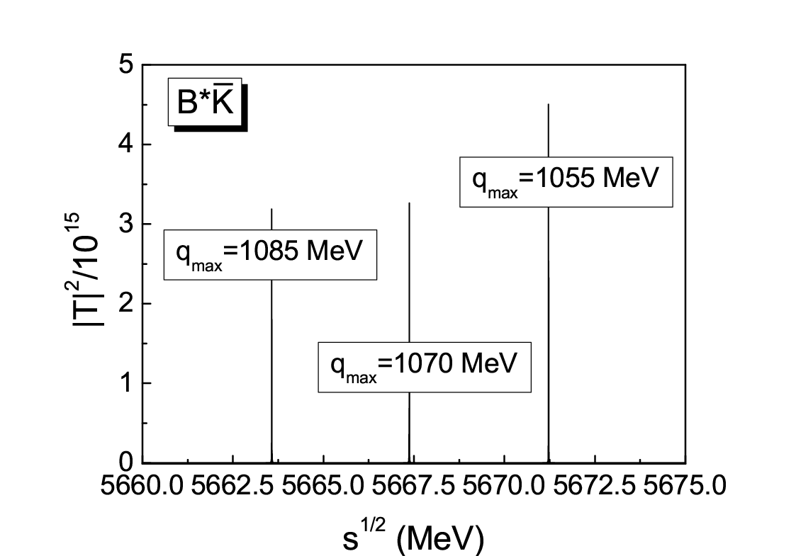
Like the case of $\bar{K}^{*}B/\omega B_{s}/\phi B_{s}$ system, there are no contact terms for $\bar{K}B^{*}/\eta B_{s}^{*}$ interaction. Only the vector meson exchange diagrams are considered. In Fig. 8, we plot the squared amplitude depending on the center-of-mass energy $\sqrt{s}$. Here, we also use the cut off $q_{max}=1055\sim 1085$ MeV as before. The pole position is located at $5671.2\sim 5663.6$ MeV. The couplings of $B^{*}\bar{K}$ and $B_{s}^{*}\eta$ are $30637$ MeV and $-13919$ MeV respectively, where we choose the cut off as 1070 MeV.

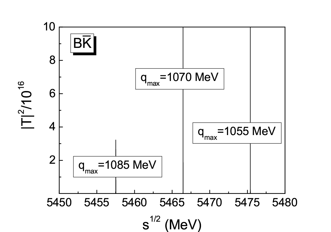
For $\bar{K}B/\eta B_{s}$ system, we predict a bound state with a mass of $5475.4\sim 5457.5$ MeV, and the couplings $g_{\bar{K}B}=53577$ MeV and $g_{\eta B_{s}}=-3689$ MeV, with a cut off $q_{max}=1070$ MeV.

In TABLE. 2, we list our results of all the systems.

References

• [1] M. Bando, T. Kugo, S. Uehara, K. Yamawaki and T. Yanagida, Phys. Rev. Lett. 54, 1215 (1985).
• [2] M. Bando, T. Kugo and K. Yamawaki, Phys. Rept. 164, 217 (1988).
• [3] U. G. Meissner, Phys. Rept. 161, 213 (1988).
• [4] M. Harada and K. Yamawaki, Phys. Rept. 381, 1 (2003)
• [5] R. Molina, D. Nicmorus and E. Oset, Phys. Rev. D 78, 114018 (2008)
• [6] L. S. Geng and E. Oset, Phys. Rev. D 79, 074009 (2009)
• [7] J. J. Xie, M. Albaladejo and E. Oset, Phys. Lett. B 728, 319 (2014)
• [8] X. L. Ren, L. S. Geng, E. Oset and J. Meng, Eur. Phys. J. A 50, 133 (2014)
• [9] R. Molina, H. Nagahiro, A. Hosaka and E. Oset, Phys. Rev. D 80, 014025 (2009)
• [10] P. del Amo Sanchez et al. [BaBar Collaboration], Phys. Rev. D 82, 111101 (2010)
• [11] R. Aaij et al. [LHCb Collaboration], JHEP 1309, 145 (2013)
• [12] R. Aaij et al. [LHCb Collaboration], Phys. Rev. D 94, no. 7, 072001 (2016)
• [13] P. Fernandez-Soler, Z. F. Sun, J. Nieves and E. Oset, Eur. Phys. J. C 76, no. 2, 82 (2016)
• [14] R. Akers et al. [OPAL Collaboration], Z. Phys. C 66, 19 (1995).
• [15] M. Moch [DELPHI Collaboration], PoS HEP 2005, 232 (2006).
• [16] R. K. Mommsen, Nucl. Phys. Proc. Suppl. 170, 172 (2007)
• [17] T. Aaltonen et al. [CDF Collaboration], Phys. Rev. Lett. 100, 082001 (2008)
• [18] V. M. Abazov et al. [D0 Collaboration], Phys. Rev. Lett. 100, 082002 (2008)
• [19] R. Aaij et al. [LHCb Collaboration], Phys. Rev. Lett. 110, no. 15, 151803 (2013)
• [20] W. H. Liang, C. W. Xiao and E. Oset, Phys. Rev. D 89, no. 5, 054023 (2014)
• [21] S. Sakai, L. Roca and E. Oset, Phys. Rev. D 96, no. 5, 054023 (2017)
• [22] A. V. Manohar and M. B. Wise, Camb. Monogr. Part. Phys. Nucl. Phys. Cosmol. 10, 1 (2000)
• [23] C. Patrignani et al. [Particle Data Group], Chin. Phys. C 40, no. 10, 100001 (2016). doi:10.1088/1674-1137/40/10/100001
• [24] E. Oset and A. Ramos, Eur. Phys. J. A 44, 445 (2010)
• [25] G. Ecker, J. Gasser, H. Leutwyler, A. Pich and E. de Rafael, Phys. Lett. B 223, 425 (1989).
• [26] H. Nagahiro, L. Roca, A. Hosaka and E. Oset, Phys. Rev. D 79, 014015 (2009)
• [27] W. H. Liang, J. M. Dias, V. R. Debastiani and E. Oset, arXiv:1711.10623 [hep-ph].
• [28] S. Okubo, Phys. Lett. 5, 165 (1963).
• [29] G. Zweig, Developments in the Quark Theory of Hadrons, Volume 1. Edited by D. Lichtenberg and S. Rosen. pp. 22-101
• [30] J. Iizuka, Prog. Theor. Phys. Suppl. 37, 21 (1966).
• [31] J. A. Oller, E. Oset and J. R. Pelaez, Phys. Rev. D 59, 074001 (1999) Erratum: [Phys. Rev. D 60, 099906 (1999)] Erratum: [Phys. Rev. D 75, 099903 (2007)]