A nonlinear Schrödinger equation for gravity-capillary water waves on arbitrary depth with constant vorticity: Part I
Abstract
A nonlinear Schrödinger equation for the envelope of two-dimensional gravity-capillary waves propagating at the free surface of a vertically sheared current of constant vorticity is derived. In this paper we extend to gravity-capillary wave trains the results of Thomas et al. (2012) and complete the stability analysis and stability diagram of Djordjevic & Redekopp (1977) in the presence of vorticity. Vorticity effect on the modulational instability of weakly nonlinear gravity-capillary wave packets is investigated. It is shown that the vorticity modifies significantly the modulational instability of gravity-capillary wave trains, namely the growth rate and instability bandwidth. It is found that the rate of growth of modulational instability of short gravity waves influenced by surface tension behaves like pure gravity waves: (i) in infinite depth, the growth rate is reduced in the presence of positive vorticity and amplified in the presence of negative vorticity, (ii) in finite depth, it is reduced when the vorticity is positive and amplified and finally reduced when the vorticity is negative. The combined effect of vorticity and surface tension is to increase the rate of growth of modulational instability of short gravity waves influenced by surface tension, namely when the vorticity is negative. The rate of growth of modulational instability of capillary waves is amplified by negative vorticity and attenuated by positive vorticity. Stability diagrams are plotted and it is shown that they are significantly modified by the introduction of the vorticity.
Keywords: NLS equation, modulational instability, vorticity, surface tension
1 Introduction
Generally, gravity-capillary waves are produced by wind which generates firstly a shear flow in the uppermost layer of the water and consequently these waves propagate in the presence of vorticity. These short waves play an important role in the initial development of wind waves, contribute to some extent to the sea surface stress and consequently participate in air-sea momentum transfer. Accurate representation of the surface stress is important in modelling and forecasting ocean wave dynamics. Furthermore, the knowledge of their dynamics at the sea surface is crucial for satellite remote sensing applications.
In this paper we consider both the effect of surface tension and vorticity due to a vertically sheared current on the modulational instability of a weakly nonlinear periodic short wave trains. Recently, Thomas et al. (2012) have derived a nonlinear Schrödinger equation for pure gravity water waves on finite depth with constant vorticity. Their main findings were (i) a restabilisation of the modulational instability for waves propagating in the presence of positve vorticity whatever the depth and (ii) the importance of the nonlinear coupling between the mean flow induced by the modulation and the vorticity. One of our aim is to extend Thomas’ investigation to the case of gravity-capillary waves propagating on a vertically sheared current.
The number of studies on the computation of steadily propagating periodic gravity waves on a vertically sheared current is important. For a review one can refer to the paper by Thomas et al. (2012). On the opposite, investigations devoted to the calculation of gravity-capillary waves in the presence of horizontal vorticity is rather meagre. One can cite Bratenberg & Brevik (1993) who used a third-order Stokes expansion for periodic gravity-capillary waves travelling on an opposing current and Hsu et al. (2016) who extended this work to the case of co- and counter-propagating waves. Kang & Broeck (2000) computed periodic and solitary gravity-capillary waves in the presence of constant vorticity on finite depth. They derived analytical solutions for small amplitude waves and numerical solutions for steeper waves. Wahlen (2006) proved the rigorous existence of periodic gravity-capillary waves in the presence of constant vorticity.
To our knowledge, the unique study concerning the modulational instability of gravity-capillary waves travelling on a verticaly sheared current is that of Hur (2017). The stability of irrotational gravity-capillary waves has been deeply investigated by several authors. Djordjevic & Redekopp (1977) and Hogan (1985) derived nonlinear envelope equations and considered the modulational instability of periodic gravity-capillary waves. Note that in the gravity-capillary range, three-wave interaction is possible whereas modulational instability corresponds to a four-wave resonant interaction. The numerical computations were extended to capillary waves by Chen & Saffman (1985) and Tiron & Choi (2012). Zhang & Melville (1986) investigated numerically the stability of gravity-capillary waves including, besides the four-wave resonant interaction, three-wave and five-wave resonant interactions. For a review on stability of irrotational gravity-capillary, one can refer to the review paper by Dias & Kharif (1999).
This study is devoted to the modulational instability of weakly nonlinear gravity-capillary wave packets propagating at the surface of a vertically sheared current of finite depth. In section 2, the governing equation are given and the nonlinear Schrödinger equation in the presence of surface tension and constant vorticity is derived by using a multiple scale method. In section 3, the linear stability analysis of a weakly nonlinear wave train is carried out as a function of the Bond number, the dispersive parameter and the intensity of the vertically sheared current.
2 Derivation of the NLS equation in the presence of surface tension and vorticity
We consider the modulational instability of weakly nonlinear surface gravity-capillary wave trains in the presence of vorticity. Our investigation is confined to two-dimensional water waves propagating in finite depth. Viscosity is disregarded and the fluid is considered incompressible. The geometry configuration is presented in figure 1.
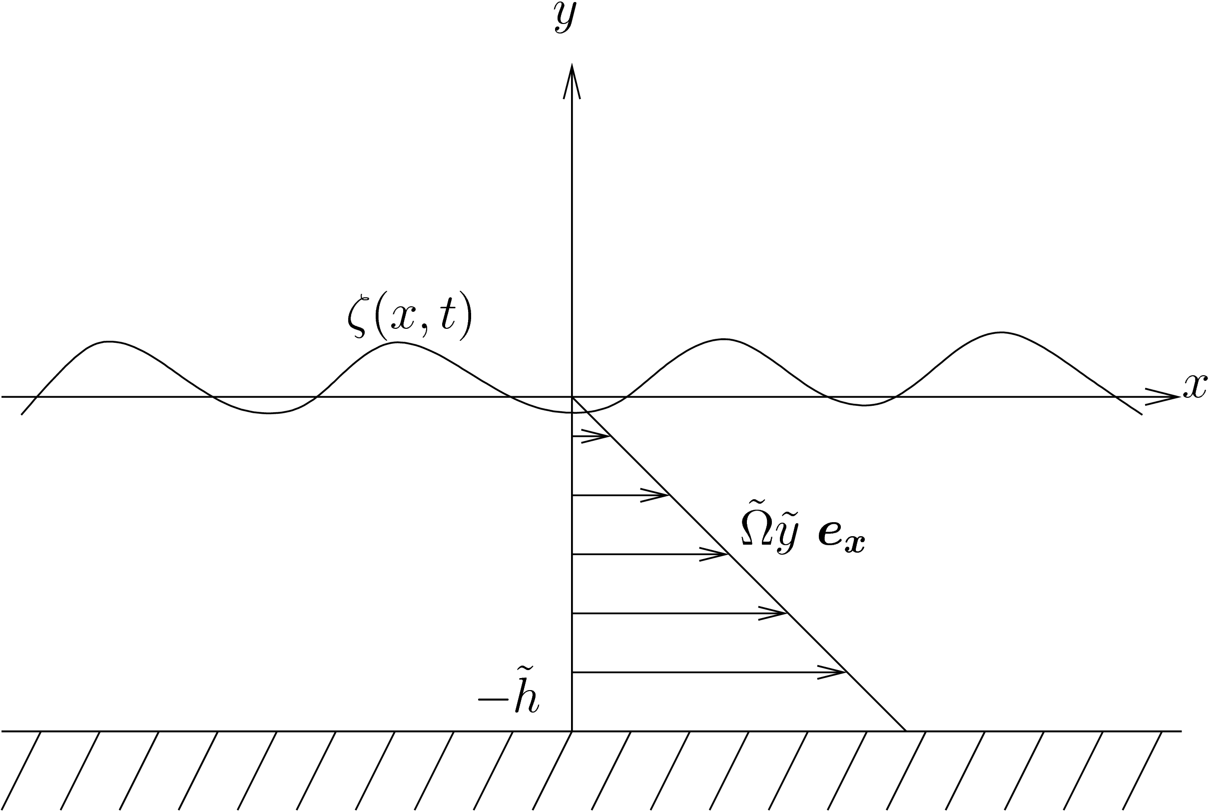
We choose an eulerian frame with unit vectors . The vector is oriented upwards so that the gravity is with . The equation of the undisturbed free surface is whereas the disturbed free surface is . The bottom is located at .
The waves are travelling at the surface of a vertically sheared current of constant vorticity. We consider an underlying current given by ,
so that the fluid velocity reads
| (1) |
where is the wave induced velocity. The waves are potential due to the Kelvin theorem which states that vorticity is conserved for a two-dimensional flow of an incompressible and inviscid fluid with external forces deriving from a potential.
The potential satisfies the Laplace equation
| (2) |
and the Euler equation can be written as follows
| (3) |
with the vorticity vector along , the pressure and the water density. Subscripts stand for derivatives in corresponding variables.
Using the Cauchy-Riemann relations
| (4) |
where is the stream function
| (5) |
The Euler equation (3) can be rewritten as follows
| (6) |
Spatial integration gives the Bernoulli equation
| (7) |
In the presence of surface tension, , at the free surface the Laplace law writes
| (8) |
where is the atmospheric pressure and surface tension.
The dynamic boundary condition at the free surface is
| (9) |
Witout loss of generality, we set and incorporate into the potential .
Along with these, we have the kinematic free surface boundary condition
| (10) |
and the bottom boundary condition
| (11) |
Following Thomas et al. (2012) we can remove by deriving (9) with respect to and then using relations (4) , keeping in mind that we are dealing with low-steepness waves, and that (9) is evaluated in , we get the equation
| (12) |
that matches the one first derived in Thomas et al. (2012) for .
Following (Davey & Stewartson, 1974), we look for solutions depending on slow variables where () and , and are the amplitude, wavenumber and group velocity of the carrier wave, respectively. The system of governing equations becomes
| (13) |
| (14) |
| (15) |
| (16) |
An asymptotic solution to the system (13-14-15-16) is sought in the following form
| (17) |
where is a plane wave with the frequency of the carrier wave. We impose that and where the bar denotes complex conjugate, so that the functions are real. The amplitudes and are then expanded in a perturbation series in terms of
| (18) |
The terms depending on surface tension occur only at a higher order. The expansions (18) are substituted into the system of equations. The linear Laplace equation (13) is easier to handle, since solutions can be derived iteratively. Here we will simply write the first order solution for , that is obtained by using the bottom boundary condition (14)
| (19) |
where the slow-varying function will be used to express all other terms. Higher-order expansions of the Laplace equation introduce more unknown functions as solutions. Nevertheless, through expansions of the boundary conditions they can be all combined to .
The evolution of this unknown will depend on the initial condition . We then use (18) in the dynamic and kinematic free surface boundary conditions, and collect terms of equal power in and , which allows the expressions for the and to be found successively.
The calculations are somewhat tedious but some steps are of interest. At first, the linear dispersion relation is derived
| (20) |
where with and .
The relation between and is the following
| (21) |
where
From the above dispersion relation we can show easily that . We note that depends also on the surface tension through and its associated dispersion relation.
It is also to be noted that the expression of the mean-flow term, which is important on the developement of the modulational instability, is similar to that of Thomas et al. (2012). Nevertheless, surface tension takes place through the phase velocity , the group velocity and .
| (22) |
and
| (23) |
Although the expressions are identical to those of Thomas et al. (2012), it should be noted that the surface tension acts through the dispersion relation, affecting , and .
It is at the order that the nonlinear Schrödinger equation is found for the potential envelope , so that
| (24) |
where the coefficients depend on .
Then the dispersion coefficient reads
| (25) | ||||
with
| (26) | |||
where is here the ratio of the group velocity to the phase velocity of the carrier. It can be expressed in a concise form
| (27) |
which depends only on . The nonlinear coefficient is
| (28) | ||||
with
| (29) | ||||
and finally
| (30) |
and we can check that these coefficients reduce to those of Djordjevic & Redekopp (1977), or Hogan (1985) in deep water, if and to those of Thomas et al. (2012) if .
The last term in brackets of equation (28) corresponds to the coupling between the mean flow due to the modulation and the vorticity which occurs at third-order. This coupling was found by Thomas et al. (2012) for the case of pure gravity waves and has an important impact on the stability analysis of progressive wave trains.
We can see that in (28) there are two possible singularities that one should avoid, either
| (31) |
which corresponds to the first gravity-capillary resonance without vorticity, or
| (32) |
which is rewritten as follows
In the absence of vorticity, the latter condition reduces to which matches the long wave - short wave resonance as shown by Davey & Stewartson (1974) and Djordjevic & Redekopp (1977). In the presence of vorticity and for pure gravity waves the nonlinear coefficient becomes singular if the following condition is satisfied
Note that this condition reduces to in the absence of vorticity.
3 Stability analysis and results
Let us write in the form
where is the envelope of the free surface elevation and denotes complex conjugation. Using (21) the NLS equation (24) is rewritten for the complex envelope as follows
| (33) |
where
The nonlinear coefficient can be written in a more compact form
In this section we consider the stability of a Stokes wave solution of the NLS equation (33) to infinitesimal disturbances.
Equation (33) admits the following solution
| (34) |
with the initial condition .
We consider infinitesimal perturbations to this solution, in amplitude and in phase , so that the perturbed
solution writes
| (35) |
Substituting this expression in the NLS equation (33), linearising and separating between real and imaginary parts, yields to a system of linear coupled partial differential equations with constant coefficients. Then, this system admits solutions of the form
| (36) |
The necessary and sufficient condition for the existence of non-trivial solutions is
| (37) |
The Stokes wave solution is stable when and unstable when
The growth rate of instability is then
We set and , so that and are dimensionless functions of , and only. The growth rate of instability becomes
| (38) |
The maximal growth rate is obtained for and its expression is . Note that instability occurs when and have opposite sign.
The growth rate of instability is written in the following dimensionless form
| (39) |
where
The dimensionless bandwidth of instability is and
.
For and , equation (39) gives the rate of growth of Thomas et al. (2012). In figure 2 is plotted the dimensionless maximal growth rate of modulational instability of pure gravity waves and gravity waves influenced by surface tension effect () as a function of for infinite and finite depths. We can observe that combined effect of surface tension and vorticity increases significantly the rate of growth of the modulational instability of short gravity waves propagating in finite depth and in the presence of negative vorticity () whereas the effect is insignificant in deep water. For positive vorticity () the curves almost coincide in finite depth and deep water as well and the increase of the rate of growth due to surface tension is of order of .

For and , equation (2.20) of Djordjevic & Redekopp (1977) becomes
for the envelope of the surface elevation in deep water.
The coefficients and corresponding to this NLS equation are
Consequently, the rate of growth of modulational instability of pure capillary wave trains on infinite depth, obtained for , is
which can be found in Chen & Saffman (1985). The wavenumber of the fastest-growing modulational instability is and the maximum growth rate is . Tiron & Choi (2012) have extended the linear stability of finite-amplitude capillary waves on deep water subject to superharmonic and subharmonic perturbations without vorticity effect.
We have considered the case of pure capillary waves on deep water ( and ) in the presence of vorticity (). The corresponding analytic expressions of and are
| (40) |
| (41) |
where and .
Due to high wave frequency of capillaries on deep water we assume . The coefficients and becomes
| (42) |
| (43) |
The rate of growth of modulational instability of capillary waves on deep water in the presence of vorticity is
| (44) |
and in dimensionless form
| (45) |
The maximal growth rate of instability is obtained for and its value is . The bandwidth of modulational instability is .
Consequently, the rate of growth of modulational instability of capillary waves in deep water is larger for negative vorticity () than for positive vorticity (). The bandwidth of instability presents the same trend.
In figure 3 is shown the dimensionless rate of growth of modulational instability of pure capillary waves in finite depth as a function of the wavenumber of the perturbation, for several values of . The rate of growth of instability increases as increases as in infinite depth.


The sign of the product determines the stability of the solution under infinitesimal perturbations. If the product is positive then the solutions are modulationally stable, otherwise they are modulationally unstable and grow exponentially with time. Davey & Stewartson (1974) and Djordjevic & Redekopp (1977) showed that this criterion which works for propagation can be extended to the case of propagation. In this way, our stability diagrams could be compared to those of Djordjevic & Redekopp (1977) when . The linear stability analysis only captures the linear part of the instability, and thus its onset. We plot in the -plane, for fixed values of the vorticity , the unstable and stable regions. As a check, the instability diagrams we obtain are compared in Figs. 4 and 5 with the same diagrams obtained by Thomas et al. (2012) for and Djordjevic & Redekopp (1977) for . In that way, we can verify that these limiting cases are reproduced correctly. Following Djordjevic & Redekopp (1977), the boundaries of the unstable regions have been numbered from 1 to 5. Curve 1 crosses the -axis at the point corresponding to restabilisation of the modulational instability. Note that this feature holds for two-dimensional water waves. Curve 2 corresponds to vanishing of the dispersive coefficient and minimum phase velocity () whereas along curves 3 and 4 the nonlinear coefficient is singular. These singularities define Wilton and long wave/short wave resonances, respectively. Curves 1 and 5 correspond to simple zeros of the nonlinear coefficient .
Curve 4 has the following asymptote
whereas curve 5 has the asymptote
For , the equations of Djordjevic & Redekopp (1977) are redicovered except that instead of we found which is slightly different. The asymptotes have the same slope. In the region beteen these two asymptotes the capillary waves () are modulationally stable. This feature was emphasized by Djordjevic & Redekopp (1977) in the absence of vorticity.
In figures 7 to 13 the effect of positive and negative vorticity on diagrams is investigated. The curves of Djordjevic & Redekopp (1977) have been plotted to show the effect of the vorticity. As it can be observed, the vorticty has a significant effect on stability diagrams of gravity-capillary. Very recently, this feature was emphasized by Hur (2017) who proposed a shallow water wave model with constant vorticity and surface tension, too. Although interesting this model suffers from shortcomings: (i) dispersion is introduced heuristically and is fully linear (ii) nonlinear terms due to surface tension effect are ignored (iii) the coupling between nonlinearity and dispersion is not taken into account.
As positive vorticity () increases, we observe in figures 7, 9, 11 and 13 along the -axis in the vicinity of an increase of the region where the Stokes gravity-capillary wave train is modulationally stable. Consequently, gravity waves influenced by surface tension behave as pure gravity waves (see Thomas et al. (2012)). Nevertheless, a very thin tongue of instability persists, near , in the shallow water regime.
As the intensity of negative vorticity () increases the band of instability along the -axis that corresponds to small values of becomes narrower, as shown in figures 7, 9, 11 and 13. Contrary to the case of positive vorticity, the region of restabilisation along the -axis does not increase in the vicinity of .


4 Conclusion
A nonlinear Schrödinger equation for capillary-gravity waves in finite depth with a linear shear current has been derived which extends the work of Thomas et al. (2012). The combined effect of vorticity and surface tension on modulational instability properties of weakly nonlinear gravity-capillary and capillary wave trains has been investigated. The explicit expressions of the dispersive and nonlinear coefficients are given as a function of the frequency and wavenumber of the carrier wave, the vorticity, the surface tension and the depth. The linear stability to modulational perturbations of the Stokes wave solution of the NLS equation has been carried out. Two kinds of waves have been especially investigated that concerns short gravity waves influenced by surface tension and pure capillary waves. In both cases, vorticity effect is to modify the rate of growth of modulational instability and instability bandwidth. Furthermore, it is shown that vorticity effect modifies significantly the stability diagrams of the gravity-capillary waves.
References
- Bratenberg & Brevik (1993) Bratenberg, C. & Brevik, I. 1993 Higher-order water waves in currents of uniform vorticity in the presence of surface tension. Phys. Scr. 47, 383–393.
- Chen & Saffman (1985) Chen, B. & Saffman, P. G. 1985 Three-dimensional stability and bifurcation of capillary and gravity waves on deep water. Stud. Appl. Math. 72, 125–147.
- Davey & Stewartson (1974) Davey, A & Stewartson, K 1974 On three-dimensional packets of surface waves. Proc. R. Soc. A A. 338, 101–110.
- Dias & Kharif (1999) Dias, F. & Kharif, C. 1999 Nonlinear gravity and capillary-gravity waves. Annu. Rev. Fluid Mech. 31, 301–346.
- Djordjevic & Redekopp (1977) Djordjevic, V.D. & Redekopp, L.G. 1977 On two-dimensional packets of capillary-gravity waves. J. Fluid Mech. 79, 703–714.
- Hogan (1985) Hogan, S. J. 1985 The fourth-order evolution equation for deep-water gravity-capillary waves. Proc. R. Soc. Lond. A 402, 359–372.
- Hsu et al. (2016) Hsu, H. C., Francius, M., Montalvo, P. & Kharif, C. 2016 Gravity-capillary waves in finite-depth on flows of constant vorticity. Proc. R. Soc. A A. 472, 20160363.
- Hur (2017) Hur, V.M. 2017 Shallow water models with constant vorticity. Eur. J. Fluids/B Fluids in press, 10.1016.
- Kang & Broeck (2000) Kang, Y. & Broeck, J-M. Vanden 2000 Gravity-capillary waves in the presence of constant vorticity. Eur. J. Fluids/B Fluids 19, 253–268.
- Thomas et al. (2012) Thomas, R., Kharif, C. & Manna, M.A. 2012 A nonlinear schrodinger equation for water waves on finite depth with constant vorticity. Phys. Fluids p. 127102.
- Tiron & Choi (2012) Tiron, R. & Choi, W. 2012 Linear stability of finite-amplitude capillary waves on water of infinite depth. J. Fluid Mech. 696, 402–422.
- Wahlen (2006) Wahlen, E. 2006 Steady periodic capillary-gravity waves with vorticity. SIAM J. Math. Anal. 38(3), 921–943.
- Zhang & Melville (1986) Zhang, J. & Melville, W.K. 1986 On the stability of weakly-nonlinear gravity-capillary waves. Wave Motion 8, 439–454.