Second order models for optimal transport and cubic splines on the Wasserstein space
Abstract.
On the space of probability densities, we extend the Wasserstein geodesics to the case of higher-order interpolation such as cubic spline interpolation. After presenting the natural extension of cubic splines to the Wasserstein space, we propose a simpler approach based on the relaxation of the variational problem on the path space. We explore two different numerical approaches, one based on multi-marginal optimal transport and entropic regularization and the other based on semi-discrete optimal transport.
1. Introduction
We propose a variational method to generalize cubic splines on the space of densities using multimarginal optimal transport. In short, the proposed method consists in minimizing, on the space of measures on the path space, under marginal constraints, the norm squared of the acceleration. In this setting, we show that two numerical approaches, classical in optimal transportation can be applied. One is based on entropic regularization and the Sinkhorn Algorithm, the other relies on the Semi-Discrete formulation of Optimal Transportation and the computation of Laguerre cells, a classical problem in computationnal geometry. We showcase our methodology on 1D and 2D data.
In the past few years, higher-order interpolations methods have been investigated for applications in computer vision or medical imaging, for time-sequence interpolation or regression. The most usual setting is when data are modeled as shapes, which can be understood as objects embedded in the Euclidean space with no preferred parametrization: space of unparametrized curves or surfaces, or images are some of the most important examples. These examples are infinite dimensional but the finite dimensional case of a Riemannian manifold was interesting for camera motion interpolation as first introduced in [22] and further developed in [6, 8]. Motivated by different applications, the problem of interpolation between two shapes is usually treated via the use of a Riemannian metric on the space of shapes and computing a geodesic between the two shapes. From a mathematical point of view, shape spaces are often infinite dimensional and thus, non-trivial analytical questions arise such as existence of minimizing geodesics or global well-posedness of the initial value problem associated with geodesics. A finite dimensional approximation is still possible such as in [29], in which spline interpolation is proposed for a diffeomorphic group action on a finite dimensional manifold. It has been extended for invariant higher-order lagrangians in [11, 12] on a group, still finite dimensional. A numerical implementation of the variational and shooting splines has been developed in [26] with applications to medical imaging. The question of existence of an extremum is not addressed in these publications. An attempt is given in [28] where the exact relaxation of the problem is computed in the case of the group of diffeomorphisms of the unit interval. In a similar direction, in [13], the authors discuss the convergence of the discretization of cubic splines in some particular infinite dimensional Riemannian context on the space of shapes.
As a shape space, we are interested in this article in probability measures endowed with the Wasserstein metric. Since the Wasserstein metric shares some similarities with a Riemannian metric on this space of probability densities, it is natural to study further higher-order models in this context. Our motivation is to answer the following practical question of the extension of cubic splines to the Wasserstein space and their numerical computation.
We present in Section 2 the notion of cubic splines on a Riemannian manifold and detail its variational formulation in Hamiltonian coordinates. We then discuss independently in Section 3 a geometric approach to the Wasserstein space that will be useful for the introduction of our proposed method detailed in Section 4. Finally in Sections 5 we present the numerical entropic relaxation method and an alternative numerical method based on semi-discrete optimal transport. The reader not interested in geometric interpretation can skip directly to Section 4.
To the best of our knowledge, this question has not been yet addressed in the literature on optimal transport until very recently in two independant and simultaneous preprints : [31] and [14] (this paper). Both work share the same idea of relaxing the cubic spline formulation in the space of measure using multi-marginal optimal transport. Our paper however explores a larger hierarchy of models and several numerical methods.
2. Cubic splines on Riemannian manifolds
In this section, we present Riemannian cubics, which are the extension of variational splines to a Riemannian manifold where is the Riemannian metric. Variational cubic splines on a Riemannian manifold are the minimizers of the acceleration; that is, denoting the covariant derivative, minimization on the set of curves of the functional
| (2.1) |
subject to constraints on the path such as constraints on the tangent space, are prescribed for a collection of times , or constraints on the positions such as .
Under mild conditions on the constraints, if is complete, minimizers exist, for instance in the case of constraints on the tangent space mentioned above. A pathological case where minimizers might not exist is when the initial speed is not prescribed. Consider for instance the two dimensional torus, where lines of irrational slopes are dense, it is possible to show that for any collection of points which do not lie on a line, the infimum of is while it is never reached, see [13]. The Euler-Lagrange equation associated to the functional is
| (2.2) |
where is the curvature tensor of the Riemannian manifold . Note that this equation is similar to a Jacobi field equation.
We now formulate the variational problem in coordinates. In a coordinate chart around a point , the geodesic equations are given by
| (2.3) |
where is a short notation for the Christoffel symbols associated with the Levi-Civita connection. It is a second-order differential equation which is conveniently written as a first-order differential equation, via the Hamiltonian formulation. Again in local coordinates on the cotangent bundle of , the geodesic equation can be written as
| (2.4) |
where . Note that, the ODE (2.3) can be obtained from the Hamiltonian system using . From these two equivalent formulations (2.3) and (2.4), it can be shown that . Therefore, it proves that the variational spline problem can be rewritten in Hamiltonian coordinates as follows
under the constraint
with initial conditions and . It is natural to ask whether such variational problems carry over in infinite dimensional situations such as the Wasserstein space, which will be discussed in the rest of the paper.
3. A formal application of spline interpolation to the Wasserstein space
It is well known that the Hamiltonian formulation of geodesics on the Wasserstein space, define over a riemannian manifold , are
| (3.1) |
where and implicitly time dependant are respectively a probability density and a function. Note that these equations are valid when working with smooth densities. The Hamiltonian is the following,
| (3.2) |
where is a reference measure on .
Remark 1.
Taking the gradient of the equation governing , and denoting , we get Burger’s equation:
| (3.3) |
where in coordinates, the operator is defined as where are vector fields and is the dimension of the . In Lagrangian coordinates, this equation implies that
| (3.4) |
where is the Lagrangian flow associated with (), which is well-defined under sufficient regularity conditions.
Remark 2.
For the Wasserstein case, the operator is given by so that the (formal) computation of the covariant derivative on the Wasserstein space is:
| (3.5) |
where is the horizontal lift associated with , that is . This result is proven rigorously in [18].
From a control viewpoint, we aim at minimizing for the control system:
| (3.6) |
where is a time dependent function defined on . Alternatively, in terms of the variables , this amounts to minimize
| (3.7) |
under the continuity equation constraint . It is a nonconvex optimization problem in the couple . The key issue here is that the variational problem itself is a priori not well-posed since our formulation is valid in a smooth setting and to make it rigorous on the space of measures, the tight relaxation of this problem is needed. However, we do not address this issue in our work and in the next section we turn our attention to a simple relaxation of the problem which is probably not tight.
4. A hierarchy of relaxed models
4.1. Context
We recall the classical optimal transport setting. We have the following well known equivalence [23, 30]
| (4.1) |
Under constraints that
( is the image measure of :
for every measurable function )
and the continuity equation
with fixed initial and final conditions
Moreover, geodesics in the space of densities for the Wasserstein metric are given by
and the associated displacement maps satisfy .
The last equality in (4.1) exactly says that the infimum among all satisfying the continuity equation at each time is achieved when is a gradient. This property is a consequence of a Riemannian submersion and is called the horizontal lift of . It is this last formulation that formally gives a Riemannian structure on the space of probability measures. See the remark 1 below for more details on the geometrical structure.
For higher-order variational problems, e.g. the minimization of the acceleration, the reduction in the last inequality does not holds true in general, even if the Riemannian submersion structure is present as shown in [12]. It means in the case of acceleration that, a priori, with the same constraint as for (4.1) :
| (4.2) |
where we have used that .
Remark 1.
From a geometrical point of view, (4.1) says the Wasserstein space can be seen, at least formally, as a homogeneous space as described in [15, Appendix 5] and originally in [23]. Consider the group of (smooth) diffeomorphisms of a closed manifold, , and the space of (smooth) probability densities . The space of densities is endowed with a action defined by the pushforward, that is to a given and , the pushforward of by is . By Moser’s lemma, this action is transitive, thus making the space of densities as a homogeneous space. More importantly, there exists a compatible Riemannian structure between and . Once having chosen a reference density , the metric on the diffeomorphism group descends to the Wasserstein metric on the space of densities, or in other words, the pushforward action is a Riemannian submersion. An important property of Riemannian submersion is that geodesics on are in correspondence with geodesics on the group, given by horizontal lift. This property is actually contained in Brenier’s polar factorization theorem, which shows that the horizontal lift is the gradient of a convex function.
4.2. The Monge formulation
In Section 3 we used the formal Riemannian structure on the set of probability measure to define an intrinsic notion of splines, (3.7) is indeed the RHS of inequality (4.2). In this section we propose a simpler alternative definition of Wasserstein splines based on the LHS of inequality (4.2).
Definition 1 (Monge formulation).
Let , and be probability measures on .
Minimize, among time dependent maps ,
| (4.3) |
under the marginal constraints . This minimizing problem is denoted by .
It is a Monge formulation of the variational problem, similar to standard optimal transport. On a Riemannian manifold , the notation stands for . By the change of variable with the map , the problem can be written in Eulerian coordinates, that is using the vector field associated with the Lagrangian map , , one aims at minimizing for
| (4.4) |
under the constraints
| (4.5) |
with the marginals constraints .
Remark 2.
Remark that formally when , this new model reduces to the formulation (3.7). Therefore, it justifies the fact that Problem (4.3) is a relaxation of (3.7). However, as already mentioned, this relaxation is probably not tight.
Another formal geometric argument in the direction of proving that the two formulations are different is that the Wasserstein space has nonnegative curvature if the underlying space has nonnegative curvature, but the space of maps in the Euclidean space is flat. Therefore, the two Euler-Lagrange equations (2.2) lead to a different evolution equations: for instance, if is the Euclidean space then the Euler-Lagrange equation for the second model is simply , which is a priori different from the splines Euler-Lagrange equation in the Wasserstein case.
4.3. The Kantorovich relaxation
Since, as is well-known in standard optimal transport, the Monge formulation is not well-posed for general given margins , we propose instead to solve yet another relaxation of the problem on the space of curves which takes the form:
Definition 2 (Kantorovich relaxation).
Let , and be probability measures on .
Minimize on the space of probability measures on the path space denoted by in short,
| (4.6) |
which is a linear functional of . The curves of densities is given by its marginals in time
| (4.7) |
is the evaluation function at time :
if then .
The notation is the image measure by the map defined by duality :
for every measurable function .
Note that is a path on while is a point on .
With these notations, the marginal constraint at given time are
| (4.8) |
By standard arguments, the Kantorovich relaxation admits minimizers under general hypothesis on the manifold , which we do not detail here. It is straightforward to check that existence of minimizers holds when .
As expected, the Kantorovich formulation is the relaxation of the Monge formulation in Definition 1.
Theorem 1.
Proof.
See the proof of a more general result in Appendix A. ∎
First we remark that we can reformulate both the Monge and Kantorovich problems on the set of cubic splines. It is the purpose of the following lemmas and corollaries, whose proofs are straightforward.
Definition 3 (Cubic interpolant).
Let be given points and be timepoints. There exists a unique cubic spline minimizing the acceleration of the curve such that . This unique curve is called cubic interpolant and is denoted by , depending implicitly on the timepoints.
Lemma 2.
When the supports of the measures are compact on , the support of every minimizing in Definition 2 is included in the set the cubic interpolants for .
Proof.
The constraints are the marginal constraints for which implies that set of paths charged by an optimal measures satisfies . In particular, any path in this set can be replaced by its minimal spline energy, the cubic interpolant . ∎
Corollary 3.
As a consequence, the set of paths charged by an optimal plan are uniformly and for every smooth function with compact support, the map is .
Proof.
The set of cubic interpolants is compact since the map is continuous from to the space of fonctions (solution of an invertible linear system) and are compact. Therefore, the set of maps are uniformly . The last point follows directly. ∎
Corollary 4.
The Kantorovich problem in Definition 2 on reduces to a multimarginal optimal transport problem, as follows, let be the continuous cost of the cubic interpolant at times , the minimization of (4.6) reduces to the minimization of
| (4.9) |
on the space of probability measures and under the marginal constraints where is the projection of the factor.
Proof.
Direct consequence of Lemma 2. ∎
Similarly
Corollary 5.
The Monge problem in Definition 1 on reduces to a Monge multimarginal optimal transport problem, as follows, let be the continuous cost of the cubic interpolant at times , the minimization of (4.3) reduces to the minimization of
| (4.10) |
on the space of path (or even cubic splines) and under the marginal constraints .
The dual formulation of the minimization problem is also well known [16, Theorem 2.1]
Definition 4 (Kantorovich dual problem ).
Let be the space of integrable -uplet. Maximize on
| (4.11) |
And the following duality results holds true:
Proposition 6.
There exists a -uplet optimal for . Moreover = and for any optimal in (4.9) there holds , almost everywhere.
A natural question is whether the solution of the Kantorovich problem is admissible in the Monge formulation (Definition 1). With the formulation reduced above the spline, given by (4.9) and (4.10), one can try to apply existing theory to answer to this question, see [16, 24] and references therein for precise criterion. However our cost does not satisfy any of those known criterion. In fact, we have the following result which proves that the relaxation to plans are necessary even in the context of Theorem 1.
Proposition 7.
(Counter Example) Given the three-marginals problems of minimizing the acceleration, there exist data such that is atomless and such that the solution of is not a (measurable) Monge map.
Proof.
Consider and the Dirac masses and and the maps that respectively pushforward onto and . These maps are uniquely determined and affine. Consider now . Then, introducing , we consider , note that it is equal to since the maps are affine.
By construction, the minimization of the acceleration for is null since it is a mixture of plans supported by straight lines. If there existed an optimal Monge solution it is necessarily supported by only one map denoted by and since the cost is null, the map at time is necessarily defined above. The preimage of (resp. ) by is a measurable set (resp. ). Then, necessarily, , and in fact, and (since the image of the map is known). Therefore, we have which is not equal to the uniform Lebesgue measure on . ∎
Remark 3.
It is an open question to prove or disprove a similar result when the final density is atomless. The counterexample explained above strongly uses the fact that the final density is a sum of Dirac masses and it might not be robust when replacing the final density by a uniform density on a small interval.
4.4. The corresponding interpolation problem on the tangent space
The relaxed problem on the space of curves can be used to define variational interpolation problem on the phase space, or more precisely on the tangent space . Since the space is contained in , one can formulate the optimal transport problem on phase space (identified with the tangent space) for the acceleration cost.
Definition 5 (Optimal transport on phase space).
Let be two probability measures on . Minimize on the space of probability measures on ,
| (4.12) |
which is a linear functional of under the marginal constraints
| (4.13) |
where is defined by .
Proposition 8 (Optimal interpolation on phase space).
The support of every optimal solution is contained in the set of cubic splines interpolating between and . Moreover if and if has density with respect to the Lebesgue measure, then the unique solution to Problem (4.12) is characterized by a map .
Remark that the optimal solution in the last part of Proposition 8 provides an interpolation on the phase space using .
Proof.
Note that this problem is very different from using the Wasserstein distance on where the tangent space is endowed with the direct product metric. Indeed, the cost does not vanish on the diagonal contrarily to the quadratic cost on .
Interestingly, let us remark that the multimarginal problem can be recast as the minimization problem on , denoting the pushforward on at times ,
| (4.15) |
under the constraints that . From the numerical point of view, this rewriting might be useful since the cost used on the multimarginal problem is now separable in time. This relaxation to the tangent space is used in the semidiscrete algorithm in Section 5.3.1. Obviously, up to the minimization on the variables , we retrieve the minimization problem since one has a cost which is defined on
| (4.16) |
where the index runs over the marginals.
5. Numerical Study
We have discussed several variational relaxation of the classical definition of splines, applied to the Wasserstein space of densities. At least two different numerical techniques from Optimal Transportation can be used in this setting. We apply the Entropic regularisation and Sinkhorn (briefly recalled in appendix B first to a simple Hermite interpolation problem (section 5.1) and then in section to the multimarginal problem (4.9). In section 5.3, we use the semi-discrete Optimal Transportation approach in the spirit of [21] directly to problem (4.6) without the time discretisation in (4.9).
5.1. Hermite interpolation
In this section, we are interested in the problem of interpolation on the phase space described in the previous. The marginals are densities defined on the tangent space . If we only specify the marginals at time and as empirical measures: and , as explained in Section 4.4, we can simplify the Kantorovich using the exact norm of the acceleration of the spline between and ), whose cost is given in Formula (4.14). Again, let us underline that this cost is not a Riemannian cost on the tangent space of since if and are close, the cost is dominated by the term which need not be zero. Then, the Kantorovich problem reduces to the minimization of
| (5.1) |
under the constraints
| (5.2) |
It is straightforward to apply entropic regularization/Sinkhorn in this case
which amounts to add, for a positive parameter , to the previous linear functional and to numerically solve the corresponding variational problem with the Sinkhorn algorithm [27, 9] (See also appendix B where Sinkhorn algorithm is detailed in the more general multimarginal case).
It is interesting to note that the choice of is more delicate than in the standard case of a quadratic distance cost.
In Figure 2, we present the convergence rate of this method with respect to two different values of and the most likely deterministic plan given the optimal plan . Note that this entropic regularization method scales with the number of points as and is valid in every dimension.
 |
 |
5.2. MultiMarginal formulation
This is the direct discretization of (4.6) which avoids working in phase space with the cost (4.16) thus enabling fast computations in 2D. In what follows, the time cylinder is discretized in time as , the product space of copies of at each of the time steps. We will use a regular time step discretization where . Using a classic finite difference approach, the time discretization of (4.6) is
| (5.3) |
where now spans the space of probability measures on representing the space of piecewise linear curves passing through at times .
A straighforward computation gives
| (5.4) |
For all times, marginals (4.7) are computed as :
| (5.5) |
In order to simplify the presentation we will assume that the marginal constraints (4.8) are set at times which coincide with times steps of the discretization (of course , meaning the number of constraint is not the same as the number of time steps).
In short, there exist such that
The constraint (4.8) becomes for all
| (5.6) |
where is the prescribed density to interpolate at time .
The simplest space discretization strategy is to use a regular cartesian grid. In dimension 2 and for and at time , the grid will be denoted for and , and will be the vectors of indices.
The time and space discretization of the problem then becomes
| (5.7) |
Where is the tensor of grid values and
| (5.8) |
The marginals (5.5) at all times are given by
| (5.9) |
The constraints (5.6) therfore becomes for all
| (5.10) |
denotes the set of indices minus .
The Entropic regularized problem is
| (5.11) |
and easier to solve. See Appendix B for a description of Sinkhorn algorithm.
Numerical Simulations
1D case:
We present, figures 3 and 4, a 1D test case to highlight some of the qualitative properties of the cubic splines interpolation on the space of densities.
| ||||||
|


We consider four interpolation time points and the corresponding data are mixture of Gaussians of different standard deviations. We use a discretization of points on the interval with time steps. The doted line represent the reconstructed density curve in time. This experiment shows that the mass can concentrate or diffuse in some situation.
Another important point here is that the entropic regularization parameter has an important impact on this concentration/diffusion effects: we show the simulations for and . In the simulation with a large , the concentration effect is not present and it is due to the diffusion on the path space.
 |
 |
 |
 |
 |
 |
2D case:
We present a 2D test case which computes a Wasserstein spline in the sense of (5.7) interpolating four Gaussian identical
densities at time 1, 5, 13, and 17, see figure 5. We use a time step and 17 time steps. The space discretization is .
The entropic regularization parameter is , note that the stability of the method depends on this parameter.
It also generates artificial diffusion as it becomes more costly top concentrate the available mass on fewer Euclidean splines between the points of the support of the
four Gaussians. We can compute the interpolating densities at intermediate times using (5.9) but is more
interesting to represent in figure 6 the contour line of the third quartile, i.e. the highest values of the densities representing 1/4 of the total mass.
Comparing with figure 7, it seems clear that the Entropy diffusion spreading pollutes the solution of the original problem (without entropic regularization).
We compare this solution with the classical Quadratic cost Optimal Transport interpolation, i.e. with the speed instead of the acceleration in the cost. More precisely taking :
| (5.12) |
As expected the mass follows respectively the linear interpolation or the Euclidean spline interpolation of the center of the Gaussians which
are represented as thick red lines in figure 5.
Finally we show the convergence of the Sinkhorn iterate for both simulations in figure 6. The convergence is much slower for the speed case but we did not optimize the implementation which does not need tensors and instead just used a degraded version of the acceleration code. This may be the reason for this strange difference.
 |
 |
 |
 |
5.3. Semi-Discrete approach
We propose another numerical scheme based on the semi-discrete approach introduced by Mérigot in [19] in dimension 2 and developed by Levy [17] in dimension 3. Here we approximate the optimal plan in the formulation (4.9) by a sum of N tensor product of diracs masses. That is .
Remark 4.
Since there is a unique corresponds between points and the spline passing through these points at time the measure can also be seen as direct masses defined over the set of splines: .
We then have to relax the constraint since cannot be absolutely continuous. It leads to the following variational problem.
Definition 6 (Semi-discrete variational problem).
Let , , and be n absolutely continuous measures. Recall that is the cost of the cubic spline passing through the points at time . Let
Then the semi-discrete variational problem, (SDV), is given by
| (5.13) |
where is the classical Wasserstein distance given by the quadratic cost.
The main drawback of this method is that, as illustrated in the numerical simulations below, the problem is not convex.
5.3.1. Implementation
In order to solve numerically the minimization problem we use the reformulation of the spline cost in the phase space, that is in , with :
| (5.14) |
where
| (5.15) |
The advantage of the formulation (5.14) is that the cost is separable in the phase space and the gradient with respect to speeds and positions is easy to compute.
We thus implement a gradient descent in the phase space using the lbfgs function in python. We compute the gradient by automatic differentiation. The Wasserstein terms in the minimization problem (5.13) depends only on the positions and are computed thanks to Mérigot Library [1] in dimension 2. To do simulations in dimension 3 one has to use Lévy Library [2]. The density constraints are given trough linear functions on a triangulation.
Remark 5.
Other problems can be addressed using similar optimization problem as in Definition 6. For instance the quadratic cost in (5.13) leads to Wasserstein interpolation. We can also interpolate with curves as smooth as we want, using for instance the norm of the derivative of order of the curve or even other classical interpolating curves.
5.3.2. Numerical simulations
We propose three numerical simulations, one to compare the qualitative results with respect to the multi marginal approach and especially Figure 5. A second one in order to illustrate the non-convexity issue and a third one for applications in images.
The rotation case: Figure 7.
In this case we compute Wasserstein splines passing through four gaussians with variance 15 and center of masses respectively with constraint parameter . The number of points is . In this case the result is a global minimizer and is not sensible to initialization. The lack of convexity is not an issue. Compare to Figure 5, this approach gives a better a approximation of the intermediate densities especially with less diffusion.

 |
 |
The crossing case: Figure 8, 9
Here we compute Wasserstein splines starting from a mixture of two gaussians with centrer and variance then passing through a gaussian with center and variance and finishing at a translation of the initial mixture. The number of points is , will value or .
We expect the global minimizer to be straight lines crossing around the middle constraint and with a low cost. Numerically depending on the initial conditions, we can recover different local minimizers, the local minimum which is reached is extremely correlated with the initial coupling. In Figure 8 we observe that changing but keeping a similar initial coupling, all points are given by a quantization of the middle density with a random enumeration and initial speed, yields to a similar local minimum.
 |
 |
Finding a good initial coupling is the hard part in order reach the global maximum. One solution is to initialize with points close to each other and a very large . Then one as to add some noise in the gradient and decreases slowly . Unfortunately we didn’t find a systematic approach for this random multi-scale method and one as to fit the parameters case by case. In Figure 9 the global minimizer is achieved by first computing the spline with a relaxed constraint, i.e. large , only for the final time ( in pratice . Then we use this result, which has the good initial coupling, as and initial condition and set for all the constraints. We also compare this results with the interpolation with a different initial condition and the Wasserstein geodesics. In all these simulations we clearly observe that particles can cross along the dynamic appart from the optimal transport inthis situation.

 |
 |
Note that this spline approach is related to the problem of finding minimal geodesics along volume preserving maps done by Mérigot and Mirebeau [20] : in their work the constraints are the Lebesgue measure, the cost is changed by the quadratic cost between two points and they have a coupling constraint. Therefore their minimization problem is also non convex but the coupling is given as a constraint so the non convexity issue didn’t rise as clearly as in this spline problem.
Image interpolation:
pour l’instant c’est pas presentable, ca passe vraiment au milieu. Je vais relancer dans la semaine mais je propose de faire une version sans.
Remark 6 (Extrapolation).
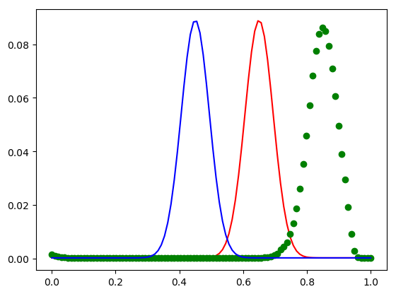
The minimization of the acceleration can be used to provide time extrapolation of Wasserstein geodesic in a natural way: particles follow straight lines. This can be implemented in a -marginal problem with the acceleration cost under marginal constraints at time and . Note that, in the spline model, the formulation we proposed does not prevent particles from crossing each other. They are completely independent. Therefore, the particles following simply geodesic lines and after a shock, the evolution is not geodesic in the Wasserstein sense (since shocks do not occur but at initial and final times). The implementation of time extrapolation using entropic regularization is straightforward. Figures 10 and 11 show some experiments on discretized with points and . The translation experiment recovers what is expected however the effect of the diffusion can be seen with a twice larger .
 |
 |
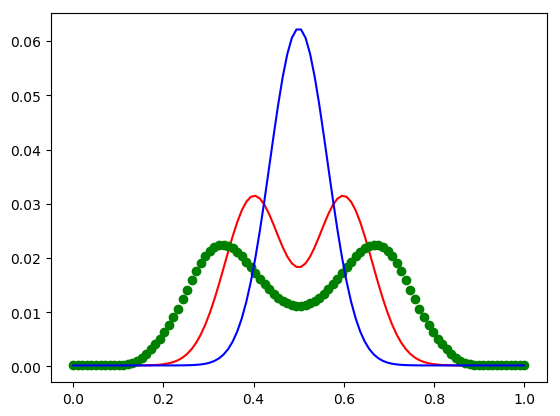
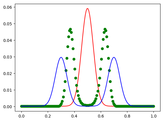
We also show two other simulations, one is a splitting simulation and the last one is a merging of two ”bumps” into a single one. The extrapolation shows an other bimodal distribution which is explained by particle crossings.
 |
 |
Note that this extrapolation scheme may proven useful in the development of higher-order schemes for the JKO algorithm.
6. Perspectives
In this paper, we presented natural approaches to define cubic splines on the space of probability measures. We have presented a Monge formulation and its Kantorovich relaxation on the path space as well as their corresponding reduction on minimal cubic spline interpolation. We leave for future work theoretical questions such as the study of conditions under which the existence of a Monge map as a minimizer occurs, as well as the relaxation of cubic spline in the Wasserstein metric. Our main contributions focus on the numerical feasibility of the minimization of the acceleration on the path space with marginal constraints. We have developed the entropic regularization scheme for the acceleration and shown simulations in 1D and 2D. Future work will address the 3D case which is out of reach with the methods presented in the first sections of this paper but possibly tackled with the semi-discrete method presented en Section 5.3. In a similar direction, the application of this approach to the unbalanced case in the spirit of [7] seems challenging due to the this dimensionality constraint and could be achieved within the semi-discrete setting.
In the Lagrangian setting, i.e. semi-discrete method, the extrapolation of a Wasserstein geodesic between and is obtained using three positions with the following formulation : let
then
| (6.1) |
where is the distance on and the cost of the cubic spline. In particular this formulation forces the curve to be a Wasserstein geodesic between and , using the quadratic cost, and let free the final marginal. The implementation is completely similar as in Section 5.3 and the trajectory of each dirac masses is a straight line.
Appendix A Proof of Theorem 1
The proof is a rewriting of the proof of [25, Theorem 1.33] when the initial and final spaces do not have the same dimension. In particular we prove that transport plans concentrated on a graph of a map are dense into transport plans in and deduce, taking , that for any continuous cost the multimarginal Kantorovich problem is the relaxation of the multimarginal Monge problem.
Theorem 9.
Let and be a continuous cost fonction. Let be probability measures on . We define the Monge Problem as
over the set of map . The Kantorovich problem is defined by
over the set of plan , where is the projection of the factor. Then, if all have compact support and is atomless there holds .
In order to prove Theorem 9 we first remark that [25, Corrollary 1.29 and Theorem 1.32 ] have their multimarginal counterpart.
Lemma 10.
Let be atomless measure and , then there exists a transport map such that .
Proof of Lemma 10.
Let (resp ) be an injective Borel map with Borel inverse (see [25, Lemma 1.28] for instance for a very simple proof of existence in this case). Since is atomless is also atomless. Let be the optimal transport map from to for the quadratic cost. . Thus is a map pushing forward to . ∎
Theorem 11.
With the notation of Theorem 9, if the support of all are included in a compact domain then the set of plans induced by a transport is dense, for the weak topology, in the set of plans whenever is atomless.
Remark 7.
Proof of Theorem 11.
Again the proof is based on [25, Theorem 1.32]. In particular the strategy of the proof is to approach a transport plan by transport maps defined on small sets on which the measure is preserved.
We consider a compact domain and such that is atomless. For any set a partition of (resp ) into (disjoint) sets (resp ) with diameter smaller than . Then is a partition of into sets with diameter smaller than . Let be the restriction of on and and . Since is atomless is also atomless and thanks to Lemma 10 there exists such that . By definition
| (A.1) |
where is define on by . In particular . Equation (A.1) and the definition of the partition sets implies that weakly converges toward as (they give same masses to any set of the partition). See [Theorem 1.31]santambrogio2015optimal for instance. To finish the proof let us remark that we can set then is atomless and defines . ∎
Appendix B Entropic Regularisation and Sinkhorn
B.1. Entropic regularization and Sinkhorn algorithm
The linear programming problems (5.7-5.10) is extremely costly to solve numerically and a natural strategy, which has received a lot of attention recently
following the pionneering works of [10] and [9] is to approximate these problems by strictly convex ones by adding an entropic penalization.
It has been used with good results on a number of multi-marginal optimal transport problems [3] [4] [5].
Here is a rapid and simplified description, see the references above for more details.
The regularized problem is
| (B.1) |
It is strictly convex. Denoting the Lagrange multipliers of the k constraints (5.10), we obtain the optimality conditions:
| (B.2) |
where
Equation (B.2) caracterize the optimal tensor as a scaling of the Kernel depending on the dual unknown . Inserting this factorization into the constrains (5.10) the dual problem takes the form of the set of equations ( )
| (B.3) |
Sinkhorn algorithm simply amounts to perform a Gauss-Seidel type iterative resolution of the system (B.3) and therefore consists in computing the sums on the right-hand side and then perform the (grid) point wise division.
B.2. Implementation
In dimension 2, each unknown has dimension , the cost of one full Gauss Seidel cycle, i.e. on Sinkhorn iteration on all unknowns, will therefore be the cost to compute the tensor matrix products in the denominator of (B.3). Remember that is the number of time steps with constraints and the total number of time steps. The given tensor Kernel is a priori a large tensor with indices . It can however advantageously be tensorized both along dimensions and also margins. First, using (5.4-5.8) we see that the Kernel is the product of smaller tensors
Moreover as we chose to work on a cartesian grid at all time steps, tensorize again into
Finally our large kernel can be represented a the product of identical tensors of size . Assuming a cubic cost for the multiplication of two matrix, we see oru algorithm is of order in dimension 2.
References
- [1] https://github.com/mrgt/PyMongeAmpere.
- [2] https://members.loria.fr/Bruno.Levy/GEOGRAM/vorpaview.html.
- [3] Jean-David Benamou, Guillaume Carlier, Marco Cuturi, Luca Nenna, and Gabriel Peyré. Iterative Bregman projections for regularized transportation problems. SIAM Journal on Scientific Computing, 37(2):A1111–A1138, 2015.
- [4] Jean-David Benamou, Guillaume Carlier, and Luca Nenna. A Numerical Method to solve Optimal Transport Problems with Coulomb Cost. working paper or preprint, May 2015.
- [5] Jean-David Benamou, Guillaume Carlier, and Luca Nenna. Generalized incompressible flows, multi-marginal transport and Sinkhorn algorithm. working paper or preprint, October 2017.
- [6] M. Camarinha, F. Silva Leite, and P.Crouch. Splines of class on non-euclidean spaces. IMA Journal of Mathematical Control & Information, 12:399–410, 1995.
- [7] L. Chizat, B. Schmitzer, G. Peyré, and F.-X. Vialard. An Interpolating Distance between Optimal Transport and Fisher-Rao. Found. Comp. Math., 2016.
- [8] P. Crouch and F. Silva Leite. The dynamic interpolation problem: On Riemannian manifold, Lie groups and symmetric spaces. Journal of dynamical & Control Systems, 1:177–202, 1995.
- [9] Marco Cuturi. Sinkhorn distances: Lightspeed computation of optimal transport. In Advances in Neural Information Processing Systems, pages 2292–2300, 2013.
- [10] Alfred Galichon and Bernard Salanié. Matching with Trade-offs: Revealed Preferences over Competiting Characteristics. working paper or preprint, April 2010.
- [11] F. Gay-Balmaz, D. D. Holm, D. M. Meier, T. S. Ratiu, and F.-X. Vialard. Invariant Higher-Order Variational Problems. Communications in Mathematical Physics, 309:413–458, January 2012.
- [12] F. Gay-Balmaz, D. D. Holm, D. M. Meier, T. S. Ratiu, and F.-X. Vialard. Invariant Higher-Order Variational Problems II. Journal of NonLinear Science, 22:553–597, August 2012.
- [13] B. Heeren, M. Rumpf, and B. Wirth. Variational time discretization of Riemannian splines. ArXiv e-prints, November 2017.
- [14] François-Xavier Vialard Jean-David Benamou, Thomas Gallouët. Second order models for optimal transport and cubic splines on the wasserstein space. Preprint arXiv:1801.04144, 2018.
- [15] B. Khesin and R. Wendt. The geometry of infinite-dimensional groups, volume 51. Springer Science & Business Media, 2008.
- [16] Young-Heon Kim and Brendan Pass. A general condition for monge solutions in the multi-marginal optimal transport problem. SIAM Journal on Mathematical Analysis, 46(2):1538–1550, 2014.
- [17] Lévy, Bruno. A numerical algorithm for l2 semi-discrete optimal transport in 3d. ESAIM: M2AN, 49(6):1693–1715, 2015.
- [18] J. Lott. Some geometric calculations on Wasserstein space. Communications in Mathematical Physics, 277(2):423–437, 2008.
- [19] Quentin Mérigot. A multiscale approach to optimal transport. Computer Graphics Forum, 30 (5):1583–1592, 2011.
- [20] Quentin Mérigot and Jean-Marie Mirebeau. Minimal geodesics along volume preserving maps, through semi-discrete optimal transport. arXiv preprint arXiv:1505.03306, 2015.
- [21] Quentin Mérigot and Jean-Marie Mirebeau. Minimal geodesics along volume-preserving maps, through semidiscrete optimal transport. SIAM J. Numer. Anal., 54(6):3465–3492, 2016.
- [22] L. Noakes, G. Heinzinger, and B. Paden. Cubic splines on curved spaces. IMA Journal of Mathematical Control & Information, 6:465–473, 1989.
- [23] F. Otto. The geometry of dissipative evolution equations: The porous medium equation. Communications in Partial Differential Equations, 26(1-2):101–174, 2001.
- [24] Pass, Brendan. Multi-marginal optimal transport: Theory and applications∗. ESAIM: M2AN, 49(6):1771–1790, 2015.
- [25] F. Santambrogio. Optimal transport for applied mathematicians. Progress in Nonlinear Differential Equations and their applications, 87, 2015.
- [26] Nikhil Singh, François-Xavier Vialard, and Marc Niethammer. Splines for diffeomorphisms. Medical Image Analysis, 25(1):56–71, 2015.
- [27] R. Sinkhorn. Diagonal equivalence to matrices with prescribed row and column sums. Amer. Math. Monthly, 74:402–405, 1967.
- [28] R. Tahraoui and F.-X. Vialard. Riemannian cubics on the group of diffeomorphisms and the Fisher-Rao metric. ArXiv e-prints, June 2016.
- [29] F.-X. Vialard and A. Trouvé. Shape Splines and Stochastic Shape Evolutions: A Second Order Point of View. Quart. Appl. Math., 2012.
- [30] Cédric Villani. Optimal transport: old and new, volume 338. Springer Science & Business Media, 2008.
- [31] Tryphon T Georgiou Yongxin Chen, Giovanni Conforti. Measure-valued spline curves: An optimal transport viewpoint. Preprint arXiv:1801.03186, 2018.