跳到论文正文
W Papers独立论文阅读器 arXiv:1801.04021 论文正文 计算阅读时间 · 0%
引用这篇论文根据当前论文元数据生成,正式投稿前建议核对。


License: arXiv.org perpetual non-exclusive license
arXiv:1801.04021v2 [math-ph] 17 Feb 2019

Analyticity of Resonances and Eigenvalues and Spectral Properties of the massless Spin-Boson Model

Miguel Ballesteros ††thanks: miguel.ballesteros@iimas.unam.mx, Instituto de Investigaciones en Matemáticas Aplicadas y en Sistemas, Universidad Nacional Autánoma de México    Dirk-André Deckert ††thanks: deckert@math.lmu.de, Mathematisches Institut der Ludwig-Maximilians-Universität München    Felix Hänle ††thanks: haenle@math.lmu.de, Mathematisches Institut der Ludwig-Maximilians-Universität München
August 24, 2026
Abstract

We extend the method of Pizzo multiscale analysis for resonances introduced in [5] in order to infer analytic properties of resonances and eigenvalues (and their eigenprojections) as well as estimates for the localization of the spectrum of dilated Hamiltonians and norm-bounds for the corresponding resolvent operators, in neighborhoods of resonances and eigenvalues. We apply our method to the massless Spin-Boson model assuming a slight infrared regularization. We prove that the resonance and the ground-state eigenvalue (and their eigenprojections) are analytic with respect to the dilation parameter and the coupling constant. Moreover, we prove that the spectrum of the dilated Spin-Boson Hamiltonian in the neighborhood of the resonance and the ground-state eigenvalue is localized in two cones in the complex plane with vertices at the location of the resonance and the ground-state eigenvalue, respectively. Additionally, we provide norm-estimates for the resolvent of the dilated Spin-Boson Hamiltonian near the resonance and the ground-state eigenvalue. The topic of analyticity of eigenvalues and resonances has let to several studies and advances in the past. However, to the best of our knowledge, this is the first time that it is addressed from the perspective of Pizzo multiscale analysis. Once the multiscale analysis is set up our method gives easy access to analyticity: Essentially, it amounts to proving it for isolated eigenvalues only and use that uniform limits of analytic functions are analytic. The type of spectral and resolvent estimates that we prove are needed to control the time evolution including the scattering regime. The latter will be demonstrated in a forthcoming publication. The introduced multiscale method to study spectral and resolvent estimates follows its own inductive scheme and is independent (and different) from the method we apply to construct resonances.

1 Introduction

In this paper, we analyze the massless Spin-Boson model which is a simple but non-trivial model of quantum field theory. It can be seen as a model of a two-level atom interacting with its second quantized scalar field, and hence, provides a widely employed model for quantum optics. The unperturbed energies of the two-level atom shall be denoted by real numbers e0<e1e_{0}<e_{1}. After switching on the interaction with a massless scalar field that may induce transitions between the atom levels, the free ground-state energy e0e_{0} is shifted to the interacting ground-state energy λ0\lambda_{0} while the free excited state with energy e1e_{1} turns into a resonance with complex energy λ1\lambda_{1}.

Unfortunately, in the massless case, neither e0e_{0} nor e1e_{1} are isolated points in the spectrum of the free Hamiltonian which is why the interacting ground-state and the resonance (λ0\lambda_{0} and λ1\lambda_{1}) cannot be constructed using standard results from regular perturbation theory. Several technologies were developed to overcome this difficulty. Two succesful methods that recently received a lot of attention are: The so-called Pizzo multiscale method (see e.g. [21, 22, 5, 4]) and the renormalization group method (see e.g. [7, 9, 8, 6, 10, 2, 15, 16, 25, 14, 12]). In both cases, a family of spectrally dilated Hamiltonians is analyzed since this allows for complex eigenvalues. In this paper, we will employ the Pizzo multiscale technique. This technique invokes an infrared cut-off which is then removed using an inductive scheme. In each step of the induction, lower and lower boson momenta are added to the interaction and regular perturbation theory is used to construct the respective ground-state and resonance. In order to reach the limit of no infrared cut-off good control over the closing gap is essential. Note that such a procedure has been introduced for the construction of resonances in the Pauli-Fierz model [4, 5]. In this work we also construct resonances (and ground-state eigenvalues) but this is not our main purpose. Our main purpose is to prove that resonances are analytic with respect to the dilation parameter and coupling constant, and furthermore, to provide certain spectral and resolvent estimates that allow for the control of the dynamics including the scattering regime. In a forthcoming paper, these estimates are employed to address scattering theory for the model at hand. We want to remark that in [11] the time evolution of this model is studied using the spectral renormalization method. Some results derived therein are similar to some of ours, however, utilizing different methods, respectively.

What we call resonances and ground-states multiscale analysis is an inductive construction of a sequence of Hamiltonians that enjoy infrared cutoffs and satisfy certain properties. As the parameter of the sequence tends to infinity these cutoffs are removed. Our mutliscale analysis is the content of Theorem 4.5. Its basic scheme is presented in Section 4.2 and the proof of Theorem 4.5 is carried out in Section 4.3. Our proofs of analyticity and of resolvent and spectral estimates are not part of our multiscale analysis employed in the contruction of the resonance and ground-state energy, they only use it as mathematical input. The latter results are presented in Section 5 (spectral and resolvent estimates) and Section 6 (analyticity). Theorem 4.5 is only an intermediate but necessary step. As we mention above, the method of multiscale analysis for resonances is introduced in [4, 5]. However, the results in [4, 5] cannot be used directly to prove analyticity because many of the estimations therein consider the dilation parameter, θ\theta, to be purely imaginary whereas analyticity requires estimates that are uniform for θ\theta in an open set. Thus, although it does not involve major obstacles, for the sake of analyticity, many of the given calculations and some of the proofs need to be redone. For the convenience of the reader and in order to keep this work self-contained we provide them in the proof of Theorem 4.5. Note that Theorem 4.5 is applied to the Spin-Boson model while [4, 5] address the Pauli-Fierz model. This gives us the opportunity to review the Pizzo multiscale technique for a non-trivial but more tractable model.

In Section 5 (in particular, in Subsection 5.1) we introduce a new inductive scheme that is used to study resolvent and spectral estimates. This scheme is independent and different from the scheme used in Section 4 to construct resonances. It allows to localize the spectrum in two cones with vertices at the location of the resonance and ground-state energy, respectively, and allows for arbitrary small apex angles provided the coupling constant is sufficiently small. We want to emphasize that such a result requires a more subtle analysis than localizing the spectrum in cuspidal domains. Additionally, we provide estimates for the resolvent operator in the vicinity of the cones.

The study of analytic properties of resonances and ground-state eigenvalues in the context of non-relativistic quantum field theory has been the source of several studies. These papers use the method of spectral renormalization. In [17] a large class of models of quantum field theory was analyzed and analyticity of the ground-state with respect to the coupling constant was proven under the assumption this ground-state is non-degenerate. The existence of a unique ground-state and its analyticity with respect to the coupling constant was shown in [19] for the Spin-Boson model without an infrared regularization, and in [18] for the Pauli-Fierz model. Furthermore, in [12], a model describing the interaction of an atom with its quantized electromagnetic field was studied and it was proven, that the excited states are analytic functions of the momentum of the atom and of the coupling constant. Likewise, in [1], it is shown that the ground-state energy of the translationally invariant Nelson model is an analytic function of the coupling constant and the total momentum.

Here, to the best of our knowledge, we give the first extension of the Pizzo multiscale method that provides a ready access to analyticity properties that essentially amounts to proving it for isolated eigenvalues only and exploiting that uniform limits of analytic functions are analytic.

In [7, 9, 8], the renormalized group technique was invented and applied in order to construct the ground state and resonances for the confined Pauli-Fierz model. Moreover, resolvent and spectral estimates were obtained therein. Based on this new method, several simplifications and applications were developed in a variety of works [6, 10, 12, 16, 15, 2, 12, 25, 14, 2]. The Pizzo multiscale analysis was first invented in [21, 22] and then adapted in order to gain access to spectral and resolvent estimates and the construction of ground-states in [4, 5]. In [11], resolvent and spectral estimates are derived in order to control the time evolution in the Spin-Boson model and, in [13], smoothness of the resolvent and local decay of the photon dynamics for quantum states in a spectral interval just above the ground state energy was proven.

Next, we will introduce the massless Spin-Boson model together with the well-known mathematical facts and tools in order to present our main results in Section 2.

1.1 The Spin-Boson model

In the rest of this Section 1 we will state preliminary definitions and well-known tools and facts from which we start our analysis.

The non-interacting Spin-Boson Hamiltonian is defined as

H0:=K⊗𝟙+𝟙⊗Hf,K:=(e100e0),Hf:=∫d3​k​ω​(k)​a​(k)∗​a​(k).\displaystyle H_{0}:=K\otimes\mathbbm{1}+\mathbbm{1}\otimes H_{f},\qquad K:=\begin{pmatrix}e_{1}&0\\ 0&e_{0}\end{pmatrix},\qquad H_{f}:=\int\mathrm{d^{3}}k\,\omega(k)a(k)^{*}a(k). (1.1)

We regard KK as an idealized free Hamiltonian of a two-level atom. As already stated in the introduction, its two energy levels are denoted by the real numbers 0=e0<e10=e_{0}<e_{1}. Furthermore, HfH_{f} denotes the free Hamiltonian of a massless scalar field having dispersion relation ω⁡(k)=|k|\omega(k)=|k|, and a,a∗a,a^{*} are the annihilation and creation operators on standard Fock space which will be defined below. In the following we will sometimes call KK the atomic part, and HfH_{f} the free field part of the Hamiltonian. The sum of the free two-level atom Hamiltonian KK and the free field Hamiltonian HfH_{f} will simply be referred to as the “free Hamiltonian” H0H_{0}. The interaction term reads

V:=σ1⊗(a⁡(f)+a​(f)∗),whereσ1=(0110),\displaystyle V:=\sigma_{1}\otimes\left(a(f)+a(f)^{*}\right),\qquad\text{where}\qquad\sigma_{1}=\begin{pmatrix}0&1\\ 1&0\end{pmatrix}, (1.2)

and the boson form factor is given by

f:ℝ3∖{0}→ℝ,k↦e−k2Λ2​|k|−12+μ.\displaystyle f:\mathbb{R}^{3}\setminus\{0\}\to\mathbb{R},\qquad k\mapsto e^{-\frac{k^{2}}{\Lambda^{2}}}|k|^{-\frac{1}{2}+\mu}. (1.3)

Given the two-point function in (1.13) the relativistic form factor is f⁡(k)=(2​π)−32​(2​|k|)−12f(k)=(2\pi)^{-\frac{3}{2}}(2|k|)^{-\frac{1}{2}} which, however, renders the model ill-defined due to the fact that such an ff is not square integrable. This is referred to as ultraviolet divergence. In our case, the Gaussian factor in (1.3) acts as an ultraviolet cut-off for Λ>0\Lambda>0 being the ultraviolet cut-off parameter and, in addition, the fixed number

μ∈(0,1/2)\displaystyle\mu\in(0,1/2) (1.4)

implies a regularization of the infrared singularity at k=0k=0 which is a technical assumption chosen to keep the proofs of this work more tractable. With a lot of additional work one can also treat the case μ=0\mu=0 using methods described in [3]. In our notation the missing factor 2−12​(2​π)−322^{-\frac{1}{2}}(2\pi)^{-\frac{3}{2}} is absorbed in the coupling constant. The full Spin-Boson Hamiltonian is then defined as

H:=H0+g​V\displaystyle H:=H_{0}+gV (1.5)

for some coupling constant g∈ℂg\in\mathbb{C}. The operator HH is densely defined on the Hilbert space

ℋ:=𝒦⊗ℱ⁡[𝔥],𝒦:=ℂ2,\displaystyle\mathcal{H}:=\mathcal{K}\otimes\mathcal{F}\left[\mathfrak{h}\right],\qquad\mathcal{K}:=\mathbb{C}^{2}, (1.6)

where

ℱ⁡[𝔥]:=⨁n=0∞ℱn​[𝔥],ℱn​[𝔥]:=𝔥⊙n,𝔥:=L2​(ℝ3,ℂ)\displaystyle\mathcal{F}\left[\mathfrak{h}\right]:=\bigoplus^{\infty}_{n=0}\mathcal{F}_{n}\left[\mathfrak{h}\right],\qquad\mathcal{F}_{n}\left[\mathfrak{h}\right]:=\mathfrak{h}^{\odot n},\qquad\mathfrak{h}:=L^{2}(\mathbb{R}^{3},\mathbb{C}) (1.7)

denotes the standard bosonic Fock space and superscript ⊙n\odot n denotes the n-th symmetric tensor product where by convention 𝔥⊙0≡ℂ\mathfrak{h}^{\odot 0}\equiv\mathbb{C}. Throughout this work we will use the notation ℕ0:=ℕ∪{0}\mathbb{N}_{0}:=\mathbb{N}\cup\{0\}. Thanks to the direct sum, an element Ψ∈ℱ⁡[𝔥]\Psi\in\mathcal{F}[\mathfrak{h}] can be represented as a family (ψn)n∈ℕ0(\psi_{n})_{n\in\mathbb{N}_{0}} of wave functions ψn∈𝔥⊙n\psi_{n}\in\mathfrak{h}^{\odot n}. The state Ψ\Psi with ψ0=1\psi_{0}=1 and ψn=0\psi_{n}=0 for all n≥1n\geq 1 is called the vacuum and is denoted by

Ω:=(1,0,0,…)∈ℱ⁡[𝔥].\displaystyle\Omega:=(1,0,0,\dots)\in\mathcal{F}\left[\mathfrak{h}\right]. (1.8)

For any h∈𝔥h\in\mathfrak{h} and Ψ=(ψn)n∈ℕ0∈ℱ⁡[𝔥]\Psi=(\psi_{n})_{n\in\mathbb{N}_{0}}\in\mathcal{F}[\mathfrak{h}], we define the creation operator

(a​(h)∗​Ψ)n∈ℕ0:=(0,h⊙ψ0,2​h⊙ψ1,…),(a​(h)∗​Ψ)n=n​h⊙ψn−1,∀n∈ℕ,\displaystyle\left(a(h)^{*}\Psi\right)_{n\in\mathbb{N}_{0}}:=\left(0,h\odot\psi_{0},\sqrt{2}h\odot\psi_{1},\dots\right),\quad\left(a(h)^{*}\Psi\right)_{n}=\sqrt{n}h\odot\psi_{n-1},\quad\forall n\in\mathbb{N}, (1.9)

and the annihilation operator a⁡(h)a(h) as the respective adjoint. Occasionally, we shall also use the physics notation

a​(h)∗=∫d3​k​h​(k)​a​(k)∗,h∈𝔥,\displaystyle a(h)^{*}=\int\mathrm{d^{3}}k\,h(k)a(k)^{*},\qquad h\in\mathfrak{h}, (1.10)

where, formally, the action of these operators in the nn boson sector of a vector Ψ=(ψn)n∈ℕ0∈ℱ⁡[𝔥]\Psi=(\psi_{n})_{n\in\mathbb{N}_{0}}\in\mathcal{F}[\mathfrak{h}] can be seen as:

(a⁡(k)​ψ)(n)​(k1,…,kn)\displaystyle\left(a(k)\psi\right)^{(n)}(k_{1},...,k_{n}) =n+1​ψ(n+1)​(k,k1,…,kn)\displaystyle=\sqrt{n+1}\psi^{(n+1)}(k,k_{1},...,k_{n}) (1.11)
(a​(k)∗​ψ)(n)​(k1,…,kn)\displaystyle\left(a(k)^{*}\psi\right)^{(n)}(k_{1},...,k_{n}) =1n​∑i=1nδ(3)​(k−ki)​ψ(n−1)​(k1,…,k~i,…,kn).\displaystyle=\frac{1}{\sqrt{n}}\sum^{n}_{i=1}\delta^{(3)}(k-k_{i})\psi^{(n-1)}(k_{1},...,\tilde{k}_{i},...,k_{n}). (1.12)

Here, the notation ⋅~\tilde{\cdot} means that the corresponding variable is omitted. Note that aa and a∗a^{*} fulfill the canonical commutation relations:

[a(h),a∗(l)]=⟨h,l⟩𝔥,[a(h),a(l)]=0,[a∗(h),a∗(l)]=0∀h,l∈𝔥.\displaystyle\left[a(h),a^{*}(l)\right]=\left\langle h,l\right\rangle_{\mathfrak{h}},\qquad\left[a(h),a(l)\right]=0,\qquad\left[a^{*}(h),a^{*}(l)\right]=0\qquad\forall h,l\in\mathfrak{h}. (1.13)

Let us recall some well-known facts about the introduced model. Clearly, KK is self-adjoint on 𝒦\mathcal{K} and its spectrum consists of two eigenvalues e0e_{0} and e1e_{1}. The corresponding eigenvectors are

φ0=(01)andφ1=(10)withK​φi=ei​φi,i=0,1.\displaystyle\varphi_{0}=\begin{pmatrix}0\\ 1\end{pmatrix}\qquad\text{and}\qquad\varphi_{1}=\begin{pmatrix}1\\ 0\end{pmatrix}\qquad\text{with}\qquad K\varphi_{i}=e_{i}\varphi_{i},\quad i=0,1. (1.14)

Moreover, HfH_{f} is self-adjoint on its natural domain 𝒟⁡(Hf)⊂ℱ⁡[𝔥]\mathcal{D}(H_{f})\subset\mathcal{F}[\mathfrak{h}] and its spectrum σ⁡(Hf)=[0,∞)\sigma(H_{f})=[0,\infty) is absolutely continuous (see [24]). Consequently, the spectrum of H0H_{0} is given by σ⁡(H0)=[e0,∞)\sigma(H_{0})=[e_{0},\infty), and e0,e1e_{0},e_{1} are eigenvalues embedded in the absolutely continuous part of the spectrum of H0H_{0} (see [23]).

Finally, also the closedness of the full Hamiltonian HH is well-known (see e.g. [20]), however, for the sake of completeness, we give a proof in the Appendix A.

Proposition 1.1.

The operator VV is relatively bounded by H0H_{0} with infinitesimal bound and, consequently, HH is a closed operator on the domain 𝒟⁡(H)=𝒦⊗𝒟⁡(Hf)\mathcal{D}(H)=\mathcal{K}\otimes\mathcal{D}(H_{f}).

Remark 1.2.

In this work we omit spelling out identities whenever unambiguous. For every vector spaces V1V_{1}, V2V_{2} and operators A1A_{1} and A2A_{2} defined on V1V_{1} and V2V_{2}, respectively, we identify

A1≡A1⊗𝟙V2,A2≡𝟙V1⊗A2.A_{1}\equiv A_{1}\otimes\mathbbm{1}_{V_{2}},\hskip 56.9055ptA_{2}\equiv\mathbbm{1}_{V_{1}}\otimes A_{2}. (1.15)

In order to simplify our notation further, and whenever unambiguous, we do not utilize specific notations for every inner product or norm that we employ.

1.1.1 Complex dilation

In the following we introduce the tools necessary for the complex dilation of Hamiltonians that allows to study resonances as eigenvalues.

Definition 1.3.

For every θ∈ℝ\theta\in\mathbb{R}, we define the unitary transformation

uθ:𝔥\displaystyle u_{\theta}:\mathfrak{h} →𝔥,ψ⁡(k)→e−3​θ2​ψ​(e−θ​k).\displaystyle\rightarrow\mathfrak{h},\qquad\psi(k)\rightarrow e^{-\frac{3\theta}{2}}\psi(e^{-\theta}k). (1.16)

Similarly, we define its second quantization Uθ:ℱ⁡[𝔥]→ℱ⁡[𝔥]U_{\theta}:\mathcal{F}[\mathfrak{h}]\rightarrow\mathcal{F}[\mathfrak{h}] by its action on ℱn​[𝔥]\mathcal{F}_{n}[\mathfrak{h}]:

Uθ​Ψ(n)​(k1,…,kn)=e−3​θ2​n​Ψ(n)​(e−θ​k1,…,e−θ​kn).\displaystyle U_{\theta}\Psi^{(n)}(k_{1},...,k_{n})=e^{-\frac{3\theta}{2}n}\Psi^{(n)}(e^{-\theta}k_{1},...,e^{-\theta}k_{n}). (1.17)

A straight forward calculation yields, for every θ∈ℝ\theta\in\mathbb{R},

aθ​(h):=Uθ​a​(h)​Uθ−1=e−32​θ​a​(hθ)wherehθ​(k):=h⁡(e−θ​k)\displaystyle a^{\theta}(h):=U_{\theta}a(h)U^{-1}_{\theta}=e^{-\frac{3}{2}\theta}a(h_{\theta})\qquad\text{where}\qquad h_{\theta}(k):=h(e^{-\theta}k) (1.18)

for h∈𝔥h\in\mathfrak{h} and (again, for θ∈ℝ\theta\in\mathbb{R})

Hθ:=Uθ​H​Uθ−1=H0θ+g​Vθ,\displaystyle H^{\theta}:=U_{\theta}HU^{-1}_{\theta}=H_{0}^{\theta}+gV^{\theta}, (1.19)

where

H0θ:=K⊗𝟙+𝟙⊗Hfθ,Hfθ=e−θ​Hf,Vθ=σ1⊗(a⁡(fθ¯)+a​(fθ)∗)\displaystyle H_{0}^{\theta}:=K\otimes\mathbbm{1}+\mathbbm{1}\otimes H^{\theta}_{f},\hskip 28.45274ptH_{f}^{\theta}=e^{-\theta}H_{f},\qquad V^{\theta}=\sigma_{1}\otimes\left(a(f^{\overline{\theta}})+a(f^{\theta})^{*}\right) (1.20)

and

fθ:ℝ3→ℝ,k↦e−θ⁡(1+μ)​e−e2​θ​k2Λ2​|k|−12+μ.\displaystyle f^{\theta}:\mathbb{R}^{3}\to\mathbb{R},\quad k\mapsto e^{-\theta(1+\mu)}e^{-e^{2\theta}\frac{k^{2}}{\Lambda^{2}}}|k|^{-\frac{1}{2}+\mu}. (1.21)

The expressions for HfθH_{f}^{\theta} and fθf^{\theta} above are well-defined for θ∈ℂ\theta\in\mathbb{C}. It follows from Appendix A that, as long as fθ,fθ/ω∈𝔥f^{\theta},f^{\theta}/\sqrt{\omega}\in\mathfrak{h}, VθV^{\theta} is relatively bounded, with infinitesimal bound, with respect to H0θH_{0}^{\theta} provided, e.g., |θ|<π/16|\theta|<\pi/16. In this case we define HθH^{\theta} using the right hand side of Eq. (1.19). Employing similar bounds as in Appendix A it turns out that HθH^{\theta} is a closed operator and 𝒟⁡(Hθ)=𝒟⁡(H0)\mathcal{D}(H^{\theta})=\mathcal{D}(H_{0}). Then, it is easy to see that the family {Hθ}|θ|<π/16\left\{H^{\theta}\right\}_{|\theta|<\pi/16} is an analytic family of type AA. Notice that the expression in the middle of (1.19) does not make sense for non-real θ\theta because we have not defined UθU_{\theta} for those θ\theta’s (we can define it, but it turns out to be an unbounded operator and therefore the meaning of the middle of (1.19) is still unclear).

From the explicit formula of H0θH_{0}^{\theta} we deduce that it has only two eigenvalues, namely e0e_{0} and e1e_{1}, and

σ(H0θ)={ei+e−θr:r≥0,i∈{0,1}}.\sigma(H_{0}^{\theta})=\Big\{e_{i}+e^{-\theta}r\>:\>r\geq 0,i\in\{0,1\}\Big\}. (1.22)

In this text we use the notation

D⁡(x,r):={z∈ℂ:|z−x|<r},x∈ℂ,r>0.\displaystyle D(x,r):=\left\{z\in\mathbb{C}:|z-x|<r\right\},\qquad x\in\mathbb{C},r>0. (1.23)

1.1.2 Infrared cut-offs and definition of the ground-state and the resonance

In the following, we introduce a family of Hamiltonians H(n),θH^{(n),\theta} which have two isolated (complex) eigenvalues λi(n)\lambda^{(n)}_{i} in small neighborhoods of eie_{i}, i∈{0,1}i\in\{0,1\}. For every nn, H(n),θH^{(n),\theta} enjoys an infared cutoff that is removed as nn tends to infinity.

Definition 1.4.

We fix a real number 𝛎∈(0,π/16)\boldsymbol{\nu}\in(0,\pi/16) and for every θ∈ℂ\theta\in\mathbb{C} we set ν:=Im⁡θ\nu:=\operatorname{Im}\theta. We define

𝒮:={θ∈ℂ:−10−3<Reθ<10−3and𝝂<Imθ<π/16}.\displaystyle\mathcal{S}:=\left\{\theta\in\mathbb{C}:-10^{-3}<\operatorname{Re}\theta<10^{-3}\quad\text{and}\quad\boldsymbol{\nu}<\operatorname{Im}\theta<\pi/16\right\}. (1.24)

For θ∈𝒮\theta\in\mathcal{S} and n∈ℕn\in\mathbb{N}, we define:

  1. (i)

    The sequence of infrared cut-offs {ρn}n∈ℕ\{\rho_{n}\}_{n\in\mathbb{N}} with ρn:=ρ0​ρn\rho_{n}:=\rho_{0}\rho^{n} for real 0<ρ0<min⁡(1,e1/4)0<\rho_{0}<\min(1,e_{1}/4) and 0<ρ<10<\rho<1. In Definition 4.2 below we specify additional properties of it.

  2. (ii)

    The cutoff-Hilbert space of one particle, 𝔥(n)\mathfrak{h}^{(n)}:

    𝔥(n):=L2​(ℝ3∖ℬρn),ℬρn:={x∈ℝ3:|x|<ρn}.\displaystyle\mathfrak{h}^{(n)}:=L^{2}(\mathbb{R}^{3}\setminus\mathcal{B}_{\rho_{n}}),\quad\mathcal{B}_{\rho_{n}}:=\left\{x\in\mathbb{R}^{3}:|x|<\rho_{n}\right\}. (1.25)

    The Fock space with one particle sector 𝔥(n)\mathfrak{h}^{(n)} is defined as in Eq. (1.7), and we denote it by ℱ⁡[𝔥(n)]\mathcal{F}[\mathfrak{h}^{(n)}]. We denote its vacuum state by Ω(n)\Omega^{(n)}. We set

    ℋ(n):=𝒦⊗ℱ⁡[𝔥(n)].\displaystyle\mathcal{H}^{(n)}:=\mathcal{K}\otimes\mathcal{F}[\mathfrak{h}^{(n)}]. (1.26)

    The free boson energy operator with an infrared cutoff is defined on ℱ⁡[𝔥(n)]\mathcal{F}[\mathfrak{h}^{(n)}] by Eq. (1.1), we denote it by Hf(n),0≡Hf(n)H_{f}^{(n),0}\equiv H_{f}^{(n)}. We set

    Hf(n),θ:=e−θ​Hf(n),0.\displaystyle H_{f}^{(n),\theta}:=e^{-\theta}H_{f}^{(n),0}. (1.27)

    For every function h∈𝔥(n)h\in\mathfrak{h}^{(n)} we define creation and annihilation operators, an​(h),an∗​(h)a_{n}(h),\,a_{n}^{*}(h), on ℱ⁡[𝔥(n)]\mathcal{F}[\mathfrak{h}^{(n)}] according to Eq. (1.10). We use the same formula for functions h∈𝔥h\in\mathfrak{h}, then it is understood that we take the restriction of hh to ℝ3∖ℬρn\mathbb{R}^{3}\setminus\mathcal{B}_{\rho_{n}}.

    We define the following family of Hamiltonians (densely defined on ℋ(n)\mathcal{H}^{(n)} - see Remark 1.2)

    H0(n),θ:=K+Hf(n),θ,V(n),θ:=σ1⊗(an​(fθ¯)+an​(fθ)∗)\displaystyle H_{0}^{(n),\theta}:=K+H^{(n),\theta}_{f},\hskip 28.45274ptV^{(n),\theta}:=\sigma_{1}\otimes\left(a_{n}(f^{\overline{\theta}})+a_{n}(f^{\theta})^{*}\right) (1.28)

    and

    H(n),θ:=H0(n),θ+g​V(n),θ.\displaystyle H^{(n),\theta}:=H_{0}^{(n),\theta}+gV^{(n),\theta}. (1.29)

The Hamiltonians H(n),θH^{(n),\theta} turn out to have gaps between the eigenvalues λi(n)\lambda^{(n)}_{i} and the rest of the spectrum of H(n),θH^{(n),\theta}. This allows us to define Riesz projections, Pi(n)P_{i}^{(n)}, corresponding to the eigenvalues λi(n)\lambda_{i}^{(n)} and use regular perturbation theory for each n∈ℕn\in\mathbb{N}. In an inductive scheme, one can obtain explicit estimates on the resolvents and the eigenvalues in each step. Below, we prove that the sequences (λi(n))n∈ℕ(\lambda^{(n)}_{i})_{n\in\mathbb{N}} converge and the interacting ground-state energy λ0\lambda_{0} and resonance energy λ1\lambda_{1} of HθH^{\theta} are the limits

λi:=limn→∞λ(n)i,i=0,1.\displaystyle\lambda_{i}:=\lim\limits_{n\to\infty}\lambda^{(n)}_{i},\qquad i=0,1. (1.30)

We define

𝔥(n,∞):=L2​(ℬρn).\displaystyle\mathfrak{h}^{(n,\infty)}:=L^{2}(\mathcal{B}_{\rho_{n}}). (1.31)

We denote the corresponding Fock space by ℱ⁡[𝔥(n,∞)]\mathcal{F}[\mathfrak{h}^{(n,\infty)}] (it is defined as in (1.7)), with vacuum state Ω(n,∞)\Omega^{(n,\infty)}. It is straightforward to verify that ℋ\mathcal{H} is isomorphic to ℋ(n)⊗ℱ⁡[𝔥(n,∞)]\mathcal{H}^{(n)}\otimes\mathcal{F}[\mathfrak{h}^{(n,\infty)}] and, therefore, we identify

ℋ≡ℋ(n)⊗ℱ⁡[𝔥(n,∞)].\displaystyle\mathcal{H}\equiv\mathcal{H}^{(n)}\otimes\mathcal{F}[\mathfrak{h}^{(n,\infty)}]. (1.32)

We prove below that the sequence (Pi(n)⊗PΩ(n,∞))n∈ℕ(P^{(n)}_{i}\otimes P_{\Omega^{(n,\infty)}})_{n\in\mathbb{N}}, where PΩ(n,∞)P_{\Omega^{(n,\infty)}} is the orthogonal projection onto the vector space generated by Ω(n,∞)\Omega^{(n,\infty)}, converges to an eigenprojection corresponding to the eigenvalue λi\lambda_{i}.

2 Main results

Here, we state the main results of our work. All proofs are presented in the next sections. In Proposition 2.1 below we state the existence of the ground-state eigenvalue and the resonance of HθH^{\theta}. A similar result, for a more complicated model (Pauli-Fierz), is proved in [4]. The strategy of proof of Proposition 2.1 is based on the methods introduced in [4] but it differs from the proof therein because, here, all our estimates must be independent of θ∈𝒮\theta\in\mathcal{S}. As emphasized earlier, the existence of the resonance and the ground-state is not our focus but is only provided in order for this work to be self-contained.

The next proposition is proved in Section 5.3.

Proposition 2.1 (Construction of the ground-state and the resonance).

For every ρ,ρ0\rho,\rho_{0} sufficiently small (see Definition 4.2) there is a constant g0>0g_{0}>0 (that depends on ρ,ρ0\rho,\rho_{0} and 𝛎\boldsymbol{\nu}) such that, for every θ∈𝒮\theta\in\mathcal{S} (see (1.24)) and every g∈D⁡(0,g0)g\in D(0,g_{0}), the (complex) number

λi:=limn→∞λ(n)i,i=0,1\displaystyle\lambda_{i}:=\lim\limits_{n\to\infty}\lambda^{(n)}_{i},\quad i=0,1 (2.1)

is an eigenvalue of HθH^{\theta} and the range of

Pi:=limn→∞P(n)i⊗PΩ(n,∞),i=0,1\displaystyle P_{i}:=\lim\limits_{n\to\infty}P^{(n)}_{i}\otimes P_{\Omega^{(n,\infty)}},\quad i=0,1 (2.2)

consists of eigenvectors corresponding to λi\lambda_{i}. An explicit formula for g0g_{0} is presented in Definition 4.3 below.

The nondegeneracy of the eigenvalues in Proposition 2.1 as well as estimates for the imaginary part of the resonance can be derived from the corresponding results for the Pauli-Fierz model in [4] and [5]. Since their proofs do not need the new features of our multiscale scheme and they are not relevant for our main results, we only state them without proofs and refer to [4].

Remark 2.2 (Fermi golden rule).

The eigenvalues λ0\lambda_{0} and λ1\lambda_{1} are non-degenerate, this follows from Section 6.4.3 in [4] (we do not repeat the proof here). The leading order of the imaginary part of the resonance λ1\lambda_{1} can be explicitly calculated. This is presented in Theorem 5.6 in [4] for the Pauli-Fierz model and, using a different method, in [10]. We do not include a proof here because it follows, for the model at hand, without much change from the proof in [4].

We assume that |g|>0|g|>0 is small enough and define

EI:=−4​π2​(e1−e0)2​|f⁡(e1−e0)|2.\displaystyle E_{I}:=-4\pi^{2}(e_{1}-e_{0})^{2}|f(e_{1}-e_{0})|^{2}. (2.3)

Then, there is a constant C(2.4)>0C_{\eqref{eq:impartres1}}>0 and a constant ϵ>0\epsilon>0 such that for all n∈ℕn\in\mathbb{N} large enough

|Im⁡λ1(n)−g2​EI|≤g2+ϵ​C(2.4).\displaystyle\left|\operatorname{Im}\lambda_{1}^{(n)}-g^{2}E_{I}\right|\leq g^{2+\epsilon}C_{\eqref{eq:impartres1}}. (2.4)

The next theorems are our main results. We prove analyticity of the resonance and the ground-state, and the corresponding eigen-projections, with respect to the dilation parameter and coupling constant.

The next theorem is proved in Section 6 (see Theorem 6.9).

Theorem 2.3 (Analyticity with respect to the dilation parameter).

For ρ,ρ0\rho,\rho_{0} sufficiently small and g∈D⁡(0,g0)g\in D(0,g_{0}) (see Proposition 2.1), the functions

𝒮∋θ↦Pi,𝒮∋θ↦λi\displaystyle\mathcal{S}\ni\theta\mapsto P_{i},\hskip 28.45274pt\mathcal{S}\ni\theta\mapsto\lambda_{i} (2.5)

are analytic. Moreover, this implies that λi​(θ)≡λi\lambda_{i}(\theta)\equiv\lambda_{i} is constant for θ∈𝒮\theta\in\mathcal{S} (see (1.24)).

Remark 2.4.

Our bounds in the inductive scheme (see Theorem 4.5 below) which are used to prove Theorem 2.3 blow up as we take ν→0\nu\to 0. We study simultaneously the cases i=0i=0 and i=1i=1 and, therefore, our estimations blow up also for i=0i=0. However, it is easy to see from our method that for i=0i=0 alone we can take θ\theta in a neighborhood of 00 and prove analyticity in this neighborhood. This implies that λ0\lambda_{0} is real, because HθH^{\theta} is selfadjoint for θ=0\theta=0. It is the ground-state energy constructed in [3, 20].

Next theorem is proved in Section 6 (Theorem 6.9).

Theorem 2.5 (Analyticity with respect to the coupling constant).

For every ρ,ρ0\rho,\rho_{0} sufficiently small and g∈D⁡(0,g0)g\in D(0,g_{0}), the functions

g↦Pi,g↦λi\displaystyle g\mapsto P_{i},\hskip 28.45274ptg\mapsto\lambda_{i} (2.6)

are analytic.

Our next two theorems provide an estimate for the spectrum of HθH^{\theta} in neighborhoods of λ0\lambda_{0} and λ1\lambda_{1}, and resolvent estimates in these neighborhoods. As discussed in the introduction, similar results on spectral estimates can be found in [7, 9, 8, 10] in which the spectrum is located in cuspidal domains using the spectral renormalization method based on the Feshbach-Schur map. Here, we localize the spectrum in cones. For every z∈ℂz\in\mathbb{C}, we define

𝒞m(z):={z+xe−i​α:x≥0,|α−ν|≤ν/m},\displaystyle\mathcal{C}_{m}(z):=\left\{z+xe^{-i\alpha}:x\geq 0,|\alpha-\nu|\leq\nu/m\right\}, (2.7)

where we assume that m≥4m\geq 4, allover this work.

The next theorem is proved in the proofs of Theorems 5.9 and 5.10 below.

Theorem 2.6 (Resolvent estimates).

There is a constant ℂ\mathbb{C} (see Definition 4.1 and (5.58)) that depends on 𝛎\boldsymbol{\nu} but not on gg nor in ρ\rho and ρ0\rho_{0} such that for every m≥4m\geq 4 and ρ,ρ0\rho,\rho_{0} sufficiently small, there exists g(m)>0g^{(m)}>0 with the following properties: for every θ∈𝒮\theta\in\mathcal{S} and g∈D⁡(0,g0)g\in D(0,g_{0}) (see Proposition 2.1) with |g|≤g(m)|g|\leq g^{(m)} ,

‖1Hθ−z‖≤16​𝑪n+1​1dist⁡(z,𝒞m​(λi)),\displaystyle\left\lVert\frac{1}{H^{\theta}-z}\right\rVert\leq 16\boldsymbol{C}^{n+1}\frac{1}{{\rm dist}(z,\mathcal{C}_{m}(\lambda_{i}))}, (2.8)

for every z∈Bi(1)∖𝒞m​(λi−2​ρn1+μ/4​e−i​ν)z\in B_{i}^{(1)}\setminus\mathcal{C}_{m}\left(\lambda_{i}-2\rho_{n}^{1+\mu/4}e^{-i\nu}\right) and

‖1Hθ−z‖≤8​𝑪n+1​1dist⁡(z,𝒞m​(λi(n))),\displaystyle\left\lVert\frac{1}{H^{\theta}-z}\right\rVert\leq 8\boldsymbol{C}^{n+1}\frac{1}{{\rm dist}(z,\mathcal{C}_{m}(\lambda_{i}^{(n)}))}, (2.9)

for every z∈Bi(1)∖𝒞m​(λi(n)−ρn1+μ/4​e−i​ν)z\in B_{i}^{(1)}\setminus\mathcal{C}_{m}\left(\lambda_{i}^{(n)}-\rho_{n}^{1+\mu/4}e^{-i\nu}\right). Here, the symbol dist{\rm dist} denotes the Euclidean distance in ℂ\mathbb{C} and Bi(1)B_{i}^{(1)} is defined in (3.5).

Explicit bounds for 𝑪\boldsymbol{C}, ρ0\rho_{0} and ρ\rho, g0g_{0} and g(m)g^{(m)} are given in Definitions 4.1, 4.2, 4.3 and Eq. (5.58), respectively. We remark that we intentionally do not provide optimal estimates because these would render the proof unnecessary opaque.

The next theorem is proved in the proof of Theorem 5.10 below.

Theorem 2.7 (Spectral estimates).

For every ρ,ρ0\rho,\rho_{0} sufficiently small, θ∈𝒮\theta\in\mathcal{S} and g∈D⁡(0,g0)g\in D(0,g_{0}) with |g|≤g(m)|g|\leq g^{(m)}, there is a neighborhood Bi(1)B_{i}^{(1)} of λi\lambda_{i} (that depends on ν\nu but not on gg) such that the spectrum of HθH^{\theta} in Bi(1)B_{i}^{(1)} is contained in 𝒞⁡(λi)\mathcal{C}(\lambda_{i}) (recall that ν\nu is the imaginary part of θ\theta). An explicit formula for Bi(1)B_{i}^{(1)} is given in (3.5).

3 Resolvent estimates far away from the spectrum and detailed analysis of H(1),θH^{(1),\theta}

In this subsection we derive resolvent estimates for H(n),θH^{(n),\theta} and HθH^{\theta} for complex numbers zz that are far away from their respective spectra. For the first Hamiltonian, H(1),θH^{(1),\theta}, having an infrared cutoff, we present resolvent estimates for points that are close to its spectrum. Here, we do not need any restrictions on the sequence {ρn}n∈ℕ\{\rho_{n}\}_{n\in\mathbb{N}} other than 0<ρ0<min⁡(1,e1/4)0<\rho_{0}<\min(1,e_{1}/4), 0<ρ<10<\rho<1. In the forthcoming sections (see Definition 4.2) we need to assume other properties for the sequence {ρn}n∈ℕ\{\rho_{n}\}_{n\in\mathbb{N}}. We emphasize that the particular choice of numbers ρn\rho_{n} does not imply any physical constraint, it only specifies the rate at which the infrared cut-off is removed.

In this section and (in the whole paper) we denote by c>0c>0 any generic (indeterminate) constant (it can change from line to line) that is independent of the parameters nn, θ\theta, ρ0\rho_{0}, ρ\rho, θ\theta, 𝝂\boldsymbol{\nu} and gg. It might depend on the set 𝒮\mathcal{S}, as a whole, but not on its elements θ∈𝒮\theta\in\mathcal{S} and nor either on the parameter 𝝂\boldsymbol{\nu}. Moreover, by stating that |g||g| is small enough, we mean that there is a constant such that uniformly for |g||g| smaller than this constant the referred statement holds true. We employ that such a constant does not depend on θ\theta and nn but it depends on the set 𝒮\mathcal{S} and on the remaining parameters (e1e_{1}, ρ0\rho_{0}, ρ\rho, μ\mu and Λ\Lambda).

3.1 Resolvent estimates far away from the spectrum

We define regions in the complex plane in which we derive resolvent estimates.

Definition 3.1.

We set δ:=e1−e0=e1\delta:=e_{1}-e_{0}=e_{1} and define the region

A:\displaystyle A: =A1∪A2∪A3,\displaystyle=A_{1}\cup A_{2}\cup A_{3}, (3.1)

where

A1:\displaystyle A_{1}: ={z∈ℂ:Re⁡z<e0−12​δ}\displaystyle=\left\{z\in\mathbb{C}:\operatorname{Re}z<e_{0}-\frac{1}{2}\delta\right\} (3.2)
A2:\displaystyle A_{2}: ={z∈ℂ:Im⁡z>18​δ​sin⁡(ν)}\displaystyle=\left\{z\in\mathbb{C}:\operatorname{Im}z>\frac{1}{8}\delta\sin(\nu)\right\} (3.3)
A3:\displaystyle A_{3}: ={z∈ℂ:Rez>e1+12δ,Imz≥−sin(ν2)(Re(z)−(e1+12δ))},\displaystyle=\left\{z\in\mathbb{C}:\operatorname{Re}z>e_{1}+\frac{1}{2}\delta,\operatorname{Im}z\geq-\sin\Big(\frac{\nu}{2}\Big)\left(\operatorname{Re}(z)-(e_{1}+\frac{1}{2}\delta)\right)\right\}, (3.4)

and for i∈{0,1}i\in\{0,1\},

Bi(1):={z∈ℂ:|Rez−ei|≤12δ,−12ρ1sin(ν)≤Imz≤18δsin(ν)}.\displaystyle B_{i}^{(1)}:=\left\{z\in\mathbb{C}:|\operatorname{Re}z-e_{i}|\leq\frac{1}{2}\delta,-\frac{1}{2}\rho_{1}\sin(\nu)\leq\operatorname{Im}z\leq\frac{1}{8}\delta\sin(\nu)\right\}. (3.5)
Refer to caption
Figure 1: Subsets of the complex plane (see Definition 3.1)

In this subsection, we estimate the resolvent of H(n),θH^{(n),\theta} and HθH^{\theta} far away from their spectra, namely in the region AA defined in (3.1). These estimates are applied for the induction basis in our inductive scheme described in Section 4.2.

Lemma 3.2.

Let θ∈𝒮\theta\in\mathcal{S} (see (1.24)) and n∈ℕn\in\mathbb{N}. There is a constant C(3.6)C_{\eqref{const:resestinA}} (independent of θ\theta, nn, gg, ρ0\rho_{0}, ρ\rho and 𝛎\boldsymbol{\nu}) such that for small enough |g||g| (depending on 𝛎\boldsymbol{\nu}), for every i∈{0,1}i\in\{0,1\}:

‖1H(n),θ−z‖≤C(3.6)sin⁡(𝝂/2)​1|ei−z|,‖1Hθ−z‖≤C(3.6)sin⁡(𝝂/2)​1|ei−z|,∀z∈A.\displaystyle\left\lVert\frac{1}{H^{(n),\theta}-z}\right\rVert\leq\frac{C_{\eqref{const:resestinA}}}{\sin(\boldsymbol{\nu}/2)}\frac{1}{|e_{i}-z|},\hskip 14.22636pt\left\lVert\frac{1}{H^{\theta}-z}\right\rVert\leq\frac{C_{\eqref{const:resestinA}}}{\sin(\boldsymbol{\nu}/2)}\frac{1}{|e_{i}-z|},\qquad\forall z\in A. (3.6)
Proof.

Let z∈Az\in A and n∈ℕn\in\mathbb{N}. Then, arguing as in Appendix A and using functional calculus, we obtain that

‖V(n),θ​1H0(n),θ−z‖\displaystyle\left\lVert V^{(n),\theta}\frac{1}{H_{0}^{(n),\theta}-z}\right\rVert ≤‖V(n),θ​1(H0(n)+1)12‖​‖H0(n)+1H0(n),θ−z‖\displaystyle\leq\left\lVert V^{(n),\theta}\frac{1}{(H_{0}^{(n)}+1)^{\frac{1}{2}}}\right\rVert\left\lVert\frac{H_{0}^{(n)}+1}{H_{0}^{(n),\theta}-z}\right\rVert
≤(‖fθ‖2+2​‖fθ/ω‖2)​supy∈[0,∞),i=0,1|ei+y+1ei+e−θ​y−z|.\displaystyle\leq\left(\left\lVert f^{\theta}\right\rVert_{2}+2\left\lVert f^{\theta}/\sqrt{\omega}\right\rVert_{2}\right)\sup_{y\in[0,\infty),i=0,1}\left|\frac{e_{i}+y+1}{e_{i}+e^{-\theta}y-z}\right|. (3.7)

Geometrical considerations imply that there is a constant c>0c>0 such that

dist({ei+e−θy:i=0,1},A)≥csin⁡(𝝂/2)(1+y)∀y≥0,\displaystyle\text{dist}\left(\{e_{i}+e^{-\theta}y:\,i=0,1\},A\right)\geq\frac{c}{\sin(\boldsymbol{\nu}/2)}(1+y)\qquad\forall y\geq 0, (3.8)

and hence, there there is a constant c>0c>0 such that

‖V(n),θ​1H0(n),θ−z‖\displaystyle\left\lVert V^{(n),\theta}\frac{1}{H_{0}^{(n),\theta}-z}\right\rVert ≤csin⁡(𝝂/2),∀z∈A.\displaystyle\leq\frac{c}{\sin(\boldsymbol{\nu}/2)},\qquad\forall z\in A. (3.9)

Then, we choose |g||g| small enough such that

‖g​V(n),θ​1H0(n),θ−z‖≤12\displaystyle\left\lVert gV^{(n),\theta}\frac{1}{H_{0}^{(n),\theta}-z}\right\rVert\leq\frac{1}{2} (3.10)

and hence,

H(n),θ−z=(1+g​V(n),θ​1H0(n),θ−z)​(H0(n),θ−z)\displaystyle H^{(n),\theta}-z=\left(1+gV^{(n),\theta}\frac{1}{H_{0}^{(n),\theta}-z}\right)\left(H_{0}^{(n),\theta}-z\right) (3.11)

is invertible for all z∈Az\in A, since A∩σ⁡(H0(n),θ)=∅A\cap\sigma(H_{0}^{(n),\theta})=\emptyset. Thanks to the particular geometry, there is a constant c>0c>0 such that |ej+y​e−θ−z|≥c​sin⁡(𝝂/2)​|ei−z||e_{j}+ye^{-\theta}-z|\geq c\sin(\boldsymbol{\nu}/2)|e_{i}-z|, for every z∈Az\in A, every j∈{0,1}j\in\{0,1\}, and every positive number yy. This and (3.11) imply

‖1H(n),θ−z‖≤2​‖1H0(n),θ−z‖=supi=0,1supy≥ρn2|ei+y​e−θ−z|≤csin⁡(𝝂/2)​|ei−z|\displaystyle\left\lVert\frac{1}{H^{(n),\theta}-z}\right\rVert\leq 2\left\lVert\frac{1}{H_{0}^{(n),\theta}-z}\right\rVert=\sup_{i=0,1}\sup_{y\geq\rho_{n}}\frac{2}{|e_{i}+ye^{-\theta}-z|}\leq\frac{c}{\sin(\boldsymbol{\nu}/2)|e_{i}-z|} (3.12)

for all z∈Az\in A, i=0,1i=0,1 and some constant c>0c>0. This completes the proof for the first equation in (3.6). Since the second equation can be shown in a very similar fashion we omit the proof here. ∎

3.2 Analysis of H(1),θH^{(1),\theta}

Lemma 3.3.

Let θ∈𝒮\theta\in\mathcal{S} (see (1.24)) and |g||g| small enough (depending on 𝛎\boldsymbol{\nu} and ρ1\rho_{1}). Then,

‖1H(1),θ−z‖≤2​‖1H0(1),θ−z‖∀z∈Ei(1),i=0,1,\displaystyle\left\lVert\frac{1}{H^{(1),\theta}-z}\right\rVert\leq 2\left\lVert\frac{1}{H_{0}^{(1),\theta}-z}\right\rVert\qquad\forall z\in E^{(1)}_{i},i=0,1, (3.13)

where

Ei(1):=Bi(1)∖D⁡(ei,ρ1​sin⁡(ν)8).\displaystyle E^{(1)}_{i}:=B^{(1)}_{i}\setminus D\left(e_{i},\frac{\rho_{1}\sin(\nu)}{8}\right). (3.14)
Proof.

Let z∈Ei(1)z\in E^{(1)}_{i} and i=0,1i=0,1. Then, we have, arguing as in Appendix A,

‖V(1),θ​1H0(1),θ−z‖≤‖V(1),θ​1(H0(1)+1)12‖​‖H0(1)+1H0(1),θ−z‖\displaystyle\left\lVert V^{(1),\theta}\frac{1}{H_{0}^{(1),\theta}-z}\right\rVert\leq\left\lVert V^{(1),\theta}\frac{1}{(H_{0}^{(1)}+1)^{\frac{1}{2}}}\right\rVert\left\lVert\frac{H_{0}^{(1)}+1}{H_{0}^{(1),\theta}-z}\right\rVert
≤(‖fθ‖2+2​‖fθ/ω‖2)​supy∈{0}∪[ρ1,∞),i=0,1|ei+y+1ei+e−θ​y−z|.\displaystyle\leq\left(\left\lVert f^{\theta}\right\rVert_{2}+2\left\lVert f^{\theta}/\sqrt{\omega}\right\rVert_{2}\right)\sup_{y\in\{0\}\cup[\rho_{1},\infty),i=0,1}\left|\frac{e_{i}+y+1}{e_{i}+e^{-\theta}y-z}\right|. (3.15)

Take y∈{0}∪[ρ1,∞)y\in\{0\}\cup[\rho_{1},\infty) and i∈{0,1}i\in\{0,1\}. It follows that

|ei+y+1ei+e−θ​y−z|=\displaystyle\left|\frac{e_{i}+y+1}{e_{i}+e^{-\theta}y-z}\right|= |ei+eθ​(ei+e−θ​y−z)+1−eθ​(ei−z)ei+e−θ​y−z|\displaystyle\left|\frac{e_{i}+e^{\theta}(e_{i}+e^{-\theta}y-z)+1-e^{\theta}(e_{i}-z)}{e_{i}+e^{-\theta}y-z}\right| (3.16)
≤\displaystyle\leq |eθ|+c​1|ei+e−θ​y−z|≤cρ1​sin⁡(ν),\displaystyle|e^{\theta}|+c\frac{1}{|e_{i}+e^{-\theta}y-z|}\leq\frac{c}{\rho_{1}\sin(\nu)},

where the last inequality is due to the considered geometry.

From (3.15) and (3.16) we obtain that there is a finite constant c>0c>0 such that

‖V(1),θ​1H0(1),θ−z‖≤cρ1​sin⁡(ν)≤cρ1​sin⁡(𝝂).\displaystyle\left\lVert V^{(1),\theta}\frac{1}{H_{0}^{(1),\theta}-z}\right\rVert\leq\frac{c}{\rho_{1}\sin(\nu)}\leq\frac{c}{\rho_{1}\sin(\boldsymbol{\nu})}. (3.17)

For |g||g| small enough (depending on ρ1\rho_{1} and 𝝂\boldsymbol{\nu}), we arrive at

‖g​V(1),θ​1H0(1),θ−z‖\displaystyle\left\lVert gV^{(1),\theta}\frac{1}{H_{0}^{(1),\theta}-z}\right\rVert ≤12,\displaystyle\leq\frac{1}{2}, (3.18)

and hence,

H(1),θ−z=(1+g​V(1),θ​1H0(1),θ−z)​(H0(1),θ−z)\displaystyle H^{(1),\theta}-z=\left(1+gV^{(1),\theta}\frac{1}{H_{0}^{(1),\theta}-z}\right)\left(H_{0}^{(1),\theta}-z\right) (3.19)

is invertible for all z∈Ei(1)z\in E^{(1)}_{i}, since Ei(1)∩σ⁡(H0(1),θ)=∅E^{(1)}_{i}\cap\sigma(H_{0}^{(1),\theta})=\emptyset. Then, we obtain

‖1H(1),θ−z‖≤2​‖1H0(1),θ−z‖,\displaystyle\left\lVert\frac{1}{H^{(1),\theta}-z}\right\rVert\leq 2\left\lVert\frac{1}{H_{0}^{(1),\theta}-z}\right\rVert, (3.20)

which completes the proof. ∎

Definition 3.4.

We define the projections

P(1)i:=−12​π​i∫γ^i(1)dz1H(1),θ−z\displaystyle P^{(1)}_{i}:=-\frac{1}{2\pi i}\int_{\hat{\gamma}^{(1)}_{i}}\mathrm{d}z\,\frac{1}{H^{(1),\theta}-z} (3.21)

and

P(1)at,i:=−12​π​i∫γ^i(1)dz1H0(1),θ−z=Pei⊗PΩ(1)\displaystyle P^{(1)}_{\text{at},i}:=-\frac{1}{2\pi i}\int_{\hat{\gamma}^{(1)}_{i}}\mathrm{d}z\,\frac{1}{H_{0}^{(1),\theta}-z}=P_{e_{i}}\otimes P_{\Omega^{(1)}} (3.22)

where

γ^i(1):[0,2​π]→ℂ,t↦ei+14​ρ1​sin⁡(ν)​ei​t,\displaystyle\hat{\gamma}^{(1)}_{i}:[0,2\pi]\to\mathbb{C},\quad t\mapsto e_{i}+\frac{1}{4}\rho_{1}\sin(\nu)e^{it}, (3.23)

PeiP_{e_{i}} is the projection onto the eigenspace space corresponding to eie_{i} of the Hamiltonian KK and PΩ(1)P_{\Omega^{(1)}} is the projection onto the vector space generated by the vacuum, Ω(1)\Omega^{(1)}, of ℱ⁡[𝔥(1)]\mathcal{F}[\mathfrak{h}^{(1)}].

Remark 3.5.

The right-hand side of Eq. (3.22) follows from the following computation:

−12​π​i∫γ^i(1)dz1H0(1),θ−z=−12​π​i∫γ^i(1)dz1H0(1),θ−z(Pei⊗PΩ(1)+Pei⊗PΩ(1)¯)\displaystyle-\frac{1}{2\pi i}\int_{\hat{\gamma}^{(1)}_{i}}\mathrm{d}z\,\frac{1}{H_{0}^{(1),\theta}-z}=-\frac{1}{2\pi i}\int_{\hat{\gamma}^{(1)}_{i}}\mathrm{d}z\,\frac{1}{H_{0}^{(1),\theta}-z}(P_{e_{i}}\otimes P_{\Omega^{(1)}}+\overline{P_{e_{i}}\otimes P_{\Omega^{(1)}}})
=Pei⊗PΩ(1)−12​π​i​∫γ^i(1)d​z​1H0(1),θ−z​Pei⊗PΩ(1)¯,\displaystyle=P_{e_{i}}\otimes P_{\Omega^{(1)}}-\frac{1}{2\pi i}\int_{\hat{\gamma}^{(1)}_{i}}\mathrm{d}z\,\frac{1}{H_{0}^{(1),\theta}-z}\overline{P_{e_{i}}\otimes P_{\Omega^{(1)}}}, (3.24)

where

Pei⊗PΩ(1)¯=Pei¯⊗1+Pei⊗PΩ(1)¯\displaystyle\overline{P_{e_{i}}\otimes P_{\Omega^{(1)}}}=\overline{P_{e_{i}}}\otimes 1+P_{e_{i}}\otimes\overline{P_{\Omega^{(1)}}} (3.25)

implies that −12​π​i∫γ^i(1)dz1H0(1),θ−zPei⊗PΩ(1)¯=0-\frac{1}{2\pi i}\int_{\hat{\gamma}^{(1)}_{i}}\mathrm{d}z\,\frac{1}{H_{0}^{(1),\theta}-z}\overline{P_{e_{i}}\otimes P_{\Omega^{(1)}}}=0.

Lemma 3.6.

Let θ∈𝒮\theta\in\mathcal{S} (see (1.24)) and let |g||g| be small enough (depending on 𝛎\boldsymbol{\nu} and ρ1\rho_{1}). Take i∈{0,1}i\in\{0,1\}. Then, there is a constant C(3.26)>0C_{\eqref{eq:pconst}}>0 (independent of θ\theta, nn, gg, ρ0\rho_{0}, ρ\rho and 𝛎\boldsymbol{\nu}) such that

‖Pi(1)−Pat,i(1)‖≤|g|​C(3.26)ρ1​sin⁡(𝝂)<1and‖Pi(1)‖≤1+|g|​C(3.26)ρ1​sin⁡(𝝂)<2,\displaystyle\left\lVert P_{i}^{(1)}-P^{(1)}_{\text{at},i}\right\rVert\leq|g|\frac{C_{\eqref{eq:pconst}}}{\rho_{1}\sin(\boldsymbol{\nu})}<1\qquad\text{and}\qquad\left\lVert P_{i}^{(1)}\right\rVert\leq 1+|g|\frac{C_{\eqref{eq:pconst}}}{\rho_{1}\sin(\boldsymbol{\nu})}<2, (3.26)

where γ^i(1)\hat{\gamma}^{(1)}_{i}, Pi(1)P_{i}^{(1)} and Pat,i(1)P^{(1)}_{\text{at},i} are introduced in Definition 3.4.

Proof.

First, we observe that

‖Pi(1)−Pat,i(1)‖\displaystyle\left\lVert P_{i}^{(1)}-P^{(1)}_{\text{at},i}\right\rVert ≤12​π​‖∫γ^i(1)d​z​(1H(1),θ−z−1H0(1),θ−z)‖.\displaystyle\leq\frac{1}{2\pi}\left\lVert\int_{\hat{\gamma}^{(1)}_{i}}\mathrm{d}z\,\left(\frac{1}{H^{(1),\theta}-z}-\frac{1}{H_{0}^{(1),\theta}-z}\right)\right\rVert. (3.27)

Note that γ^i(1)⊂Ei(1)\hat{\gamma}^{(1)}_{i}\subset E^{(1)}_{i} (see (3.14)). Eq. (3.17) implies that there is a finite constant c>0c>0 such that for every zz in the (image of the) curve γ^i(1)\hat{\gamma}^{(1)}_{i}

‖g​V(1),θ​1H0(1),θ−z‖\displaystyle\left\lVert gV^{(1),\theta}\frac{1}{H_{0}^{(1),\theta}-z}\right\rVert <|g|​cρ1​sin⁡(𝝂)≤12,\displaystyle<|g|\frac{c}{\rho_{1}\sin(\boldsymbol{\nu})}\leq\frac{1}{2}, (3.28)

for |g||g| small enough (depending on 𝝂\boldsymbol{\nu} and ρ1\rho_{1}). Next, we obtain

‖Pi(1)−Pat,i(1)‖≤12​π​‖∫γ^i(1)d​z​1H0(1),θ−z​∑l=1∞(−g​V(1),θ​1H0(1),θ−z)l‖\displaystyle\left\lVert P_{i}^{(1)}-P^{(1)}_{\text{at},i}\right\rVert\leq\frac{1}{2\pi}\left\lVert\int_{\hat{\gamma}^{(1)}_{i}}\mathrm{d}z\,\frac{1}{H_{0}^{(1),\theta}-z}\sum^{\infty}_{l=1}\left(-gV^{(1),\theta}\frac{1}{H_{0}^{(1),\theta}-z}\right)^{l}\right\rVert
≤ρ1​sin⁡(ν)4​sup|z−ei|=ρ1​sin⁡(ν)4(‖1H0(1),θ−z‖)​|g|​cρ1​sin⁡(𝝂)​∑l=0∞(12)l<|g|​cρ1​sin⁡(𝝂).\displaystyle\leq\frac{\rho_{1}\sin(\nu)}{4}\sup_{|z-e_{i}|=\frac{\rho_{1}\sin(\nu)}{4}}\Big(\Big\|\frac{1}{H_{0}^{(1),\theta}-z}\Big\|\Big)|g|\frac{c}{\rho_{1}\sin(\boldsymbol{\nu})}\sum^{\infty}_{l=0}\Big(\frac{1}{2}\Big)^{l}<|g|\frac{c}{\rho_{1}\sin(\boldsymbol{\nu})}. (3.29)

This proves the first part of the lemma. Furthermore, it follows from (3.22) that ‖Pat,i(1)‖=1\left\lVert P^{(1)}_{\text{at},i}\right\rVert=1, and hence,

‖Pi(1)‖≤‖Pat,i(1)‖+‖P^i(1)−Pat,i(1)‖≤1+|g|​cρ1​sin⁡(𝝂)<2,\displaystyle\left\lVert P_{i}^{(1)}\right\rVert\leq\left\lVert P^{(1)}_{\text{at},i}\right\rVert+\left\lVert\hat{P}_{i}^{(1)}-P^{(1)}_{\text{at},i}\right\rVert\leq 1+|g|\frac{c}{\rho_{1}\sin(\boldsymbol{\nu})}<2, (3.30)

for sufficiently small |g||g|. This proves proves the second part of the lemma. ∎

Remark 3.7.

Let θ∈𝒮\theta\in\mathcal{S} (see (1.24)) and i∈{0,1}i\in\{0,1\}. Suppose that |g||g| is small enough (depending on 𝛎\boldsymbol{\nu} and ρ1\rho_{1}). Then, it follows from Lemma 3.6 together with the fact that Pat,i(1)P^{(1)}_{\text{at},i} is a rank-one projection that also Pi(1)P_{i}^{(1)} is a rank-one projection. Lemma 3.3 implies that H(1),θH^{(1),\theta} has no spectral points in Ei(1)=Bi(1)∖D⁡(ei,ρ1​sin⁡(ν)8)E_{i}^{(1)}=B^{(1)}_{i}\setminus D\left(e_{i},\frac{\rho_{1}\sin(\nu)}{8}\right). Since the contour of integration for the projection Pi(1)P_{i}^{(1)} is contained in Bi(1)B^{(1)}_{i} and its interior contains D⁡(ei,ρ1​sin⁡(ν)8)D\left(e_{i},\frac{\rho_{1}\sin(\nu)}{8}\right), we conclude that there is a unique spectral point λi(1)\lambda^{(1)}_{i} of H(1),θH^{(1),\theta} in Bi(1)B_{i}^{(1)}, it is a simple eigenvalue and it is contained in D⁡(ei,ρ1​sin⁡(ν)8)D\left(e_{i},\frac{\rho_{1}\sin(\nu)}{8}\right).

Lemma 3.3 together with Lemma 3.6 yield a resolvent estimate in the whole region Bi(1)∖{λi(1)}B_{i}^{(1)}\setminus\{\lambda_{i}^{(1)}\} by making use of the maximum modulus principle of complex analysis.

Lemma 3.8.

Let θ∈𝒮\theta\in\mathcal{S} (see (1.24)) let |g||g| be small enough (depending on 𝛎\boldsymbol{\nu} and ρ1\rho_{1}). Take i∈{0,1}i\in\{0,1\}. Then, there is a constant C(3.31)>0C_{\eqref{eq.ib-res}}>0 (independent of θ\theta, nn, gg, ρ0\rho_{0}, ρ\rho and 𝛎\boldsymbol{\nu}) such that

‖1H(1),θ−z​Pi(1)¯‖≤C(3.31)ρ1​sin⁡(ν)≤C(3.31)ρ1​sin⁡(𝝂),∀z∈Bi(1).\displaystyle\left\lVert\frac{1}{H^{(1),\theta}-z}\overline{P_{i}^{(1)}}\right\rVert\leq\frac{C_{\eqref{eq.ib-res}}}{\rho_{1}\sin(\nu)}\leq\frac{C_{\eqref{eq.ib-res}}}{\rho_{1}\sin(\boldsymbol{\nu})},\qquad\forall z\in B_{i}^{(1)}. (3.31)
Proof.

Note that the function

D⁡(ei,18​ρ1​sin⁡(ν))¯∋z↦Gϕ,ψ​(z):=⟨ϕ,1H(1),θ−z​Pi(1)¯​ψ⟩\displaystyle\overline{D\left(e_{i},\frac{1}{8}\rho_{1}\sin(\nu)\right)}\ni z\mapsto G_{\phi,\psi}(z):=\left\langle\phi,\frac{1}{H^{(1),\theta}-z}\overline{P_{i}^{(1)}}\psi\right\rangle (3.32)

is continuous, and furthermore, analytic on D⁡(ei,18​ρ1​sin⁡(ν))D\left(e_{i},\frac{1}{8}\rho_{1}\sin(\nu)\right), for all ϕ,ψ∈ℋ\phi,\psi\in\mathcal{H}. Then, it follows from the maximum modulus principle that this function attains its maximum on the boundary of its domain. This together with the Cauchy-Schwarz inequality and Lemma 3.3 and 3.6 implies that there is a finite constant c>0c>0 such that

|Gϕ,ψ​(z)|≤cρ1​sin⁡(ν)|ϕ​‖ψ‖,∀z∈D⁡(ei,18​ρ1​sin⁡(ν))¯.\displaystyle\left|G_{\phi,\psi}(z)\right|\leq\frac{c}{\rho_{1}\sin(\nu)}\|\phi\|\psi\|,\qquad\forall z\in\overline{D\left(e_{i},\frac{1}{8}\rho_{1}\sin(\nu)\right)}. (3.33)

Consequently, there is a finite constant c>0c>0 such that

‖1H(1),θ−z​Pi(1)¯‖\displaystyle\left\lVert\frac{1}{H^{(1),\theta}-z}\overline{P_{i}^{(1)}}\right\rVert ≤cρ1​sin⁡(ν),∀z∈D⁡(ei,18​ρ1​sin⁡(ν))¯,\displaystyle\leq\frac{c}{\rho_{1}\sin(\nu)},\qquad\forall z\in\overline{D\left(e_{i},\frac{1}{8}\rho_{1}\sin(\nu)\right)}, (3.34)

and moreover, Lemma 3.3 (again) guarantees that there is a finite constant c>0c>0 such that

‖1H(1),θ−z‖\displaystyle\left\lVert\frac{1}{H^{(1),\theta}-z}\right\rVert ≤2​‖1H0(1),θ−z‖≤cρ1​sin⁡(ν),\displaystyle\leq 2\left\lVert\frac{1}{H_{0}^{(1),\theta}-z}\right\rVert\leq\frac{c}{\rho_{1}\sin(\nu)}, (3.35)

for all z∈Bi(1)∖D⁡(ei,18​ρ1​sin⁡(ν))z\in B^{(1)}_{i}\setminus D\left(e_{i},\frac{1}{8}\rho_{1}\sin(\nu)\right). This together with (3.34) completes the proof. ∎

Applying Lemma 3.8 to our particular geometry allows to formulate the following corollary.

Corollary 3.9.

We define qi(1):=λi(1)+14​ρ1​e−i​νq^{(1)}_{i}:=\lambda^{(1)}_{i}+\frac{1}{4}\rho_{1}e^{-i\nu} and recall Eq. (2.7). Let θ∈𝒮\theta\in\mathcal{S} ( see (1.24)) let |g||g| be small enough (depending on 𝛎\boldsymbol{\nu} and ρ1\rho_{1}). Take i∈{0,1}i\in\{0,1\}. Then, there is a constant C(3.36)>0C_{\eqref{coroeq.ib-res}}>0 (independent of θ\theta, nn, gg, ρ0\rho_{0}, ρ\rho and 𝛎\boldsymbol{\nu}) such that

‖1H(1),θ−z​Pi(1)¯‖≤1sin⁡(ν/m)​C(3.31)dist⁡(z,𝒞m​(q1(1))),∀z∈Bi(1)∖𝒞m​(qi(1)).\displaystyle\left\lVert\frac{1}{H^{(1),\theta}-z}\overline{P_{i}^{(1)}}\right\rVert\leq\frac{1}{\sin(\nu/m)}\frac{C_{\eqref{eq.ib-res}}}{{\rm dist}(z,\mathcal{C}_{m}(q_{1}^{(1)}))},\qquad\forall z\in B^{(1)}_{i}\setminus\mathcal{C}_{m}(q_{i}^{(1)}). (3.36)
Lemma 3.10.

Let θ∈𝒮\theta\in\mathcal{S} (see (1.24)) and let |g||g| be small enough (depending on 𝛎\boldsymbol{\nu} and ρ1\rho_{1}). Then, there is a constant C(3.37)>0C_{\eqref{constgggg}}>0 (independent of θ\theta, nn, gg, ρ0\rho_{0}, ρ\rho and 𝛎\boldsymbol{\nu}) such that for every i∈{0,1}i\in\{0,1\}

|λi(1)−ei|≤|g|​C(3.37).\displaystyle\left|\lambda_{i}^{(1)}-e_{i}\right|\leq|g|C_{\eqref{constgggg}}. (3.37)
Proof.

It follows from Lemma 3.6 that |⟨φi⊗Ω,Pi(1)​φi⊗Ω⟩|>12\Big|\left\langle\varphi_{i}\otimes\Omega,P^{(1)}_{i}\varphi_{i}\otimes\Omega\right\rangle\Big|>\frac{1}{2} for |g||g| small enough (depending on 𝝂\boldsymbol{\nu} and ρ1\rho_{1}). We calculate

λi(1)\displaystyle\lambda_{i}^{(1)} =⟨φi⊗Ω(1),H(1),θ​Pi(1)​φi⊗Ω(1)⟩⟨φi⊗Ω(1),Pi(1)​φi⊗Ω(1)⟩=ei+g​⟨V(1),θ¯​φi⊗Ω(1),Pi(1)​φi⊗Ω(1)⟩⟨φi⊗Ω(1),Pi(1)​φi⊗Ω(1)⟩.\displaystyle=\frac{\left\langle\varphi_{i}\otimes\Omega^{(1)},H^{(1),\theta}P^{(1)}_{i}\varphi_{i}\otimes\Omega^{(1)}\right\rangle}{\left\langle\varphi_{i}\otimes\Omega^{(1)},P^{(1)}_{i}\varphi_{i}\otimes\Omega^{(1)}\right\rangle}=e_{i}+g\frac{\left\langle V^{(1),\overline{\theta}}\varphi_{i}\otimes\Omega^{(1)},P^{(1)}_{i}\varphi_{i}\otimes\Omega^{(1)}\right\rangle}{\left\langle\varphi_{i}\otimes\Omega^{(1)},P^{(1)}_{i}\varphi_{i}\otimes\Omega^{(1)}\right\rangle}. (3.38)

Let now z∈ℂz\in\mathbb{C} such that |ei−z|=14​ρ1​sin⁡(ν)|e_{i}-z|=\frac{1}{4}\rho_{1}\sin(\nu). Eq. (3.26) (which requires |g||g| to be small enough -depending on 𝝂\boldsymbol{\nu} and ρ1\rho_{1}) then allows to obtain

|λi(1)−ei|≤4​‖g​V(1),θ¯​φi⊗Ω(1)‖≤4​|ei−z|​‖g​V(1),θ¯​1H0(1),θ¯−z‖≤|g|​c,\displaystyle\left|\lambda_{i}^{(1)}-e_{i}\right|\leq 4\left\lVert gV^{(1),\overline{\theta}}\varphi_{i}\otimes\Omega^{(1)}\right\rVert\leq 4\left|e_{i}-z\right|\left\lVert gV^{(1),\overline{\theta}}\frac{1}{H^{(1),\overline{\theta}}_{0}-z}\right\rVert\leq|g|c, (3.39)

for some constant cc (independent of θ\theta, nn, gg, ρ0\rho_{0}, ρ\rho and 𝝂\boldsymbol{\nu}) . Here, we have used (3.17) from Lemma 3.3 in the last step. Notice that in this work we assume that the imaginary part of θ\theta, ν\nu, is positive. Then, strictly speaking, we do not have the right to use our results for θ¯\overline{\theta}. However, the restriction we impose by assuming that ν\nu is not negative is irrelevant. This is assumed only for convenience in order to simplify our notation. Of course, the same results hold true if we take −π/16<ν<−𝝂-\pi/16<\nu<-\boldsymbol{\nu}. In this case the spectrum of H0(1),θH_{0}^{(1),\theta} is just mirrored with respect to the real line. Hence, one has to mirror also the definition of Bi(1)B_{i}^{(1)} with respect to the real line in order to obtain the same estimates. Afterwards, the proofs are just the same. ∎

Remark 3.11.

Let θ∈𝒮\theta\in\mathcal{S} (see (1.24)) and let |g||g| be small enough (depending on 𝛎\boldsymbol{\nu} and ρ1\rho_{1}). Then

Pi(1)=−12​π​i∫γi(1)dz1H(1),θ−z,\displaystyle P_{i}^{(1)}=-\frac{1}{2\pi i}\int_{\gamma^{(1)}_{i}}\mathrm{d}z\,\frac{1}{H^{(1),\theta}-z}, (3.40)

where γi(1):[0,2​π]→ℂ,t↦λi(1)+14​ρ1​sin⁡(ν)​ei​t\gamma^{(1)}_{i}:[0,2\pi]\to\mathbb{C},\quad t\mapsto\lambda^{(1)}_{i}+\frac{1}{4}\rho_{1}\sin(\nu)e^{it}. This follows from Remark 3.7, because, for small enough |g||g|, γi(1),γ^i(1)⊂Bi(1)∖{λi(1)}\gamma^{(1)}_{i},\hat{\gamma}^{(1)}_{i}\subset B_{i}^{(1)}\setminus\{\lambda_{i}^{(1)}\}, see Lemma 3.10.

Lemma 3.12.

Let θ∈𝒮\theta\in\mathcal{S} (see (1.24)) and let |g||g| be small enough (depending on 𝛎\boldsymbol{\nu} and ρ1\rho_{1}). Take i∈{0,1}i\in\{0,1\}. Then, there is a constant C(3.41)>0C_{\eqref{eq.ib-resprima}}>0 (independent of θ\theta, nn, gg, ρ0\rho_{0}, ρ\rho and 𝛎\boldsymbol{\nu}) such that

‖1H(1),θ−z​Pi(1)¯‖≤C(3.41)sin⁡(𝝂)​1ρ1+|λi(1)−z|,∀z∈Bi(1).\displaystyle\left\lVert\frac{1}{H^{(1),\theta}-z}\overline{P_{i}^{(1)}}\right\rVert\leq\frac{C_{\eqref{eq.ib-resprima}}}{\sin(\boldsymbol{\nu})}\frac{1}{\rho_{1}+\left|\lambda^{(1)}_{i}-z\right|},\qquad\forall z\in B_{i}^{(1)}. (3.41)
Proof.

We use Lemma 3.8 and calculate, for |z−ei|≤ρ1|z-e_{i}|\leq\rho_{1},

1ρ1​sin⁡(ν)=ρ1+|λi(1)−z|ρ1​sin⁡(ν)​1ρ1+|λi(1)−z|≤csin⁡(𝝂)​1ρ1+|λi(1)−z|,\displaystyle\frac{1}{\rho_{1}\sin(\nu)}=\frac{\rho_{1}+|\lambda_{i}^{(1)}-z|}{\rho_{1}\sin(\nu)}\frac{1}{\rho_{1}+|\lambda_{i}^{(1)}-z|}\leq\frac{c}{\sin(\boldsymbol{\nu})}\frac{1}{\rho_{1}+|\lambda_{i}^{(1)}-z|}, (3.42)

where we use Lemma 3.10 and choose |g||g| small enough. For |z−ei|>ρ1|z-e_{i}|>\rho_{1} we use Lemma 3.3. The spectral theorem and the explicit form of the spectrum of non-interacting Hamiltonian H0(1),θH_{0}^{(1),\theta} allow us to estimate the norm of its resolvent. Then, similar estimates as above imply the desired result. ∎

Lemma 3.13.

Let θ∈𝒮\theta\in\mathcal{S} (see (1.24)) and n∈ℕn\in\mathbb{N}. There is a constant C(3.43)C_{\eqref{const:resestinAprima}} (independent of θ\theta, nn, gg, ρ0\rho_{0}, ρ\rho and 𝛎\boldsymbol{\nu}) such that for small enough |g||g| (depending on 𝛎\boldsymbol{\nu}), for every i∈{0,1}i\in\{0,1\}:

‖1H(n),θ−z‖≤C(3.43)sin⁡(𝝂/2)​1ρl+|λ~i−z|,‖1Hθ−z‖≤C(3.43)sin⁡(𝝂/2)​1ρl+|λ~i−z|,\displaystyle\left\lVert\frac{1}{H^{(n),\theta}-z}\right\rVert\leq\frac{C_{\eqref{const:resestinAprima}}}{\sin(\boldsymbol{\nu}/2)}\frac{1}{\rho_{l}+\left|\widetilde{\lambda}_{i}-z\right|},\hskip 14.22636pt\left\lVert\frac{1}{H^{\theta}-z}\right\rVert\leq\frac{C_{\eqref{const:resestinAprima}}}{\sin(\boldsymbol{\nu}/2)}\frac{1}{\rho_{l}+\left|\widetilde{\lambda}_{i}-z\right|}, (3.43)

for every z∈A∪(B1(1)−[0,∞)​e−i​ν)∖B1(1),z\in A\cup\Big(B^{(1)}_{1}-[0,\infty)e^{-i\nu}\Big)\setminus B^{(1)}_{1}, every l∈ℕl\in\mathbb{N} and every λ~i∈D⁡(λi(1),3​g).\widetilde{\lambda}_{i}\in D(\lambda^{(1)}_{i},3g).

Moreover,

‖1H(n),θ−z​Pi(1)¯‖≤1sin⁡(ν/m)​C(3.44)dist⁡(z,𝒞m​(q1(n))),\displaystyle\left\lVert\frac{1}{H^{(n),\theta}-z}\overline{P_{i}^{(1)}}\right\rVert\leq\frac{1}{\sin(\nu/m)}\frac{C_{\eqref{coroeq.ib-resT}}}{{\rm dist}(z,\mathcal{C}_{m}(q_{1}^{(n)}))}, (3.44)

for every z∈(B1(1)−[0,∞)​e−i​ν)∖B1(1)z\in\Big(B^{(1)}_{1}-[0,\infty)e^{-i\nu}\Big)\setminus B^{(1)}_{1}.

Proof.

We take z∈Az\in A. Lemma 3.10 implies that |λ~i−ei|≤|g|(C(3.37)+3)|\widetilde{\lambda}_{i}-e_{i}|\leq|g|(C_{\eqref{constgggg}}+3). Notice that

1|ei−z|≤ρm+|λ~i−z||ei−z|​1ρm+|λ~i−z|≤\displaystyle\frac{1}{|e_{i}-z|}\leq\frac{\rho_{m}+|\widetilde{\lambda}_{i}-z|}{|e_{i}-z|}\frac{1}{\rho_{m}+|\widetilde{\lambda}_{i}-z|}\leq ρm+|λ~i−ei|+|ei−z||ei−z|​1ρm+|λ~i−z|\displaystyle\frac{\rho_{m}+|\widetilde{\lambda}_{i}-e_{i}|+|e_{i}-z|}{|e_{i}-z|}\frac{1}{\rho_{m}+\left|\widetilde{\lambda}_{i}-z\right|} (3.45)
≤\displaystyle\leq c​1ρm+|λ~i−z|,\displaystyle c\frac{1}{\rho_{m}+\left|\widetilde{\lambda}_{i}-z\right|},

since |ei−z||e_{i}-z| is bounded from below uniformly for z∈Az\in A. Then, the result follows from Lemma 3.2. The result for z∈(B1(1)−[0,∞)​e−i​ν)z\in\Big(B^{(1)}_{1}-[0,\infty)e^{-i\nu}\Big) can be found similarly which is why we omit the proof. The proof of (3.44) follows from a similar argument as in Corollary 3.9,and therefore, it is also omitted. ∎

Definition 3.14.

In this subsection (Section 3) we assumed a finite number of times that |g||g| is small enough (depending on 𝛎\boldsymbol{\nu} and ρ1\rho_{1}). We set 𝐠>0\boldsymbol{g}>0 such that for every |g|≤𝐠|g|\leq\boldsymbol{g} all results of this section hold true. Similarly, in the statements of our results we use a finite number of times constants (that are independent of θ\theta, nn, gg, ρ0\rho_{0}, ρ\rho and 𝛎\boldsymbol{\nu}) in order to estimate from above norms of various entities. We denote by 𝐜≥1\boldsymbol{c}\geq 1 a, fixed, upper bound of the set of all these constants. We additionally take 𝐠\boldsymbol{g} small enough such that

‖Pi(1)−Pat,i(1)‖<10−3,\left\lVert P_{i}^{(1)}-P^{(1)}_{\text{at},i}\right\rVert<10^{-3},

see Lemma 3.6.

4 Resonance and ground-state multiscale analysis

4.1 Notation: the sequence (ρn)n∈ℕ∪{0}(\rho_{n})_{n\in\mathbb{N}\cup\{0\}} and the coupling constant gg

Next, we introduce a constant, 𝑫\boldsymbol{D}, that includes all constants involved in estimations for our multiscale construction. This constant does not depend on θ∈𝒮\theta\in\mathcal{S}, gg, 𝝂\boldsymbol{\nu}, nn, ρ\rho and ρ0\rho_{0}. Our bounds do depend on 𝝂\boldsymbol{\nu}. They blow up as 𝝂\boldsymbol{\nu} tends to zero with a rate that is not worse than sin⁡(𝝂/2)−3\sin(\boldsymbol{\nu}/2)^{-3}. The constant 𝑫\boldsymbol{D} does not depend on 𝝂\boldsymbol{\nu}. The dependence on 𝝂\boldsymbol{\nu} in our bounds is reflected in a function 𝑪≡𝑪⁡(𝝂)\boldsymbol{C}\equiv\boldsymbol{C}(\boldsymbol{\nu}) that is bounded from below by the constant 𝑫\boldsymbol{D} multiplied by the factor sin⁡(𝝂/2)−3\sin(\boldsymbol{\nu}/2)^{-3}. As already explained, the constant 𝑫\boldsymbol{D} and the blow-up rate sin⁡(𝝂/2)−3\sin(\boldsymbol{\nu}/2)^{-3} are intentionally not optimal but often estimated from above to increase the readability of the proofs.

Definition 4.1 (The function 𝑪≡𝑪⁡(𝝂)\boldsymbol{C}\equiv\boldsymbol{C}(\boldsymbol{\nu})).

We fix a constant, 𝐃\boldsymbol{D}, that does not depend on g∈D⁡(0,𝐠)g\in D(0,\boldsymbol{g}), θ∈𝒮\theta\in\mathcal{S}, and 𝛎\boldsymbol{\nu}. The only property that it must satisfy is the following (see Definition 3.14)

𝑫≥106+10​𝒄.\displaystyle\boldsymbol{D}\geq 10^{6}+10\boldsymbol{c}. (4.1)

Next, we fix a function 𝐂≡𝐂⁡(𝛎)\boldsymbol{C}\equiv\boldsymbol{C}(\boldsymbol{\nu}) satisfying

𝑪≡𝑪(𝝂)≥𝑫sin(𝝂/2)−3.\displaystyle\boldsymbol{C}\equiv\boldsymbol{C}(\boldsymbol{\nu})\geq\boldsymbol{D}\sin(\boldsymbol{\nu}/2)^{-3}. (4.2)

The sequence (ρn)n∈ℕ0(\rho_{n})_{n\in\mathbb{N}_{0}} that we introduce above is defined in the following manner.

Definition 4.2 ( Parameters ρ0\rho_{0} and ρ\rho).

The parameters ρ0\rho_{0} and ρ\rho in the definition of the sequence ρn=ρ0​ρn,n∈ℕ0\rho_{n}=\rho_{0}\rho^{n},n\in\mathbb{N}_{0}, see Definition 1.4(i), have to fulfill the following constraints:

𝑪8​ρ0μ≤1,𝑪4​ρμ≤1/4.\displaystyle\boldsymbol{C}^{8}\rho_{0}^{\mu}\leq 1,\qquad\boldsymbol{C}^{4}\rho^{\mu}\leq 1/4. (4.3)

We recall that in this work we require |g||g| to be small enough. The next definition summarizes all requirements that it must satisfy.

Definition 4.3 (The coupling constant gg).

We set a constant g0≤𝐠g_{0}\leq\boldsymbol{g} satisfying the following (see Definition 3.14):

g0≤ρ1sin(𝝂/2)2104​𝒄.\displaystyle g_{0}\leq\frac{\rho_{1}\sin(\boldsymbol{\nu}/2)^{2}}{10^{4}\boldsymbol{c}}. (4.4)

Henceforth, we always require |g|≤g0|g|\leq g_{0}.

Remark 4.4.

The selection of 𝐂\boldsymbol{C}, the sequence (ρn)n∈ℕ0(\rho_{n})_{n\in\mathbb{N}_{0}} and the constant g0g_{0} will later allow to set up the infrared induction scheme, and is therefore, rather involved. This remark is intended to help the reader to understand this procedure. Below (in this section), we use boldface fonts whenever we use the properties of 𝐂\boldsymbol{C} and gg (or g0g_{0}) that we specified above.

The requirements for (ρn)n∈ℕ0(\rho_{n})_{n\in\mathbb{N}_{0}} are only present in order to satisfy the last inequalities in Eqs. (4.7) and (4.11) below. Then, it will turn out that it is only necessary to assume that 𝐂4​ρ0μ≤1\boldsymbol{C}^{4}\rho_{0}^{\mu}\leq 1 and 𝐂2​ρμ≤1/2\boldsymbol{C}^{2}\rho^{\mu}\leq 1/2 in order to close our induction. We assume stronger conditions again, for notational convenience, and because it implies a faster convergence rate in (4.11), which will be used in a forthcoming paper (see Remark 5.11).

4.2 Induction scheme and the strategy of our multiscale construction

We denote by

𝔥(n,n+1):=L2​(ℬρn∖ℬρn+1)\displaystyle\mathfrak{h}^{(n,n+1)}:=L^{2}(\mathcal{B}_{\rho_{n}}\setminus\mathcal{B}_{\rho_{n+1}}) (4.5)

the Hilbert space of one-particle (boson) states with energies in the interval [ρn+1,ρn).[\rho_{n+1},\rho_{n}). We denote the corresponding Fock space by ℱ⁡[𝔥(n,n+1)]\mathcal{F}[\mathfrak{h}^{(n,n+1)}] (it is defined as in (1.7)). Note that ℋ(n+1)\mathcal{H}^{(n+1)} is isomorphic to ℋ(n)⊗ℱ⁡[𝔥(n,n+1)]\mathcal{H}^{(n)}\otimes\mathcal{F}[\mathfrak{h}^{(n,n+1)}], and, therefore, we identify

ℋ(n+1)≡ℋ(n)⊗ℱ⁡[𝔥(n,n+1)].\displaystyle\mathcal{H}^{(n+1)}\equiv\mathcal{H}^{(n)}\otimes\mathcal{F}[\mathfrak{h}^{(n,n+1)}]. (4.6)

For i=0,1i=0,1, we inductively (and simultaneously) construct sequences {λi(n)}n∈ℕ0\{\lambda^{(n)}_{i}\}_{n\in\mathbb{N}_{0}} of complex numbers, sequences {Bi(n)}n∈ℕ\{B^{(n)}_{i}\}_{n\in\mathbb{N}} of subsets of the complex plane and sequences {Pi(n)}n∈ℕ0\{P^{(n)}_{i}\}_{n\in\mathbb{N}_{0}} of operators that satisfy the properties listed below.

  1. (𝒫​1\mathcal{P}1)

    We set λi(0)≡λi(1)\lambda^{(0)}_{i}\equiv\lambda^{(1)}_{i}. For n∈ℕn\in\mathbb{N}, λi(n)\lambda^{(n)}_{i} is a simple eigenvalue of H(n),θH^{(n),\theta} and

    |λi(n)−λi(n−1)|<|g|​ℂn+1​(ρn−1)1+μ≤|g|​(12)n−1​ρn−1.\displaystyle\left|\lambda^{(n)}_{i}-\lambda^{(n-1)}_{i}\right|<|g|\mathbb{C}^{n+1}(\rho_{n-1})^{1+\mu}\leq|g|\left(\frac{1}{2}\right)^{n-1}\rho_{n-1}. (4.7)

    The second inequality follows from Definition 4.2.

  2. (𝒫​2\mathcal{P}2)

    For n∈ℕn\in\mathbb{N}, we define (recall that ν=Im⁡θ\nu=\operatorname{Im}\theta)

    Bi(n):=Bi(1)∖{z∈ℂ:Im⁡z<Im⁡λi(n)−14​ρn​sin⁡(ν)}.\displaystyle B_{i}^{(n)}:=B^{(1)}_{i}\setminus\left\{z\in\mathbb{C}:\operatorname{Im}z<\operatorname{Im}\lambda^{(n)}_{i}-\frac{1}{4}\rho_{n}\sin(\nu)\right\}. (4.8)

    λi(n)\lambda^{(n)}_{i} is the only point in the spectrum of H(n),θH^{(n),\theta} intersected with Bi(n)B_{i}^{(n)}.

  3. (𝒫​3\mathcal{P}3)

    We set Pi(0)≡Pi(1)P^{(0)}_{i}\equiv P^{(1)}_{i}. For n∈ℕn\in\mathbb{N}, we define

    P(n)i=−12​π​i∫γi(n)dz1H(n),θ−z,\displaystyle P^{(n)}_{i}=-\frac{1}{2\pi i}\int_{\gamma^{(n)}_{i}}\mathrm{d}z\,\frac{1}{H^{(n),\theta}-z}, (4.9)

    where

    γi(n):[0,2​π]→ℂ,t↦λi(n)+14​ρn​sin⁡(ν)​ei​t.\displaystyle\gamma^{(n)}_{i}:[0,2\pi]\to\mathbb{C},\quad t\mapsto\lambda^{(n)}_{i}+\frac{1}{4}\rho_{n}\sin(\nu)e^{it}. (4.10)

    The projections Pi(n)P^{(n)}_{i} satisfy

    ‖Pi(n)−Pi(n−1)⊗PΩ(n−1,n)‖≤|g|ρ​ℂ2​n+2​ρn−1μ≤|g|ρ​(12)n−1,\displaystyle\left\lVert P^{(n)}_{i}-P^{(n-1)}_{i}\otimes P_{\Omega^{(n-1,n)}}\right\rVert\leq\frac{|g|}{\rho}\mathbb{C}^{2n+2}\rho^{\mu}_{n-1}\leq\frac{|g|}{\rho}\left(\frac{1}{2}\right)^{n-1}, (4.11)

    where PΩ(n−1,n)P_{\Omega^{(n-1,n)}} is the projection onto the vacuum vector Ω(n−1,n)∈ℱ⁡[𝔥(n−1,n)]\Omega^{(n-1,n)}\in\mathcal{F}[\mathfrak{h}^{(n-1,n)}] (see (4.5)-(4.6)). In (4.11) we omit the tensor product for n=1n=1. The second inequality follows from Definition 4.2.

  4. (𝒫​4\mathcal{P}4)

    Set n∈ℕn\in\mathbb{N}. For any z∈Bi(n)z\in B_{i}^{(n)}, we have that

    ‖1H(n),θ−z​Pi(n)¯‖≤ℂn+1ρn+|z−λi(n)|,\displaystyle\left\lVert\frac{1}{H^{(n),\theta}-z}\overline{P^{(n)}_{i}}\right\rVert\leq\frac{\mathbb{C}^{n+1}}{\rho_{n}+\left|z-\lambda^{(n)}_{i}\right|}, (4.12)

    where Pi(n)¯=𝟙ℋ(n)−Pi(n)\overline{P^{(n)}_{i}}=\mathbbm{1}_{\mathcal{H}^{(n)}}-P^{(n)}_{i}.

Theorem 4.5 (Multiscale analysis for resonances and ground state eigenvalues).

For every i∈{0,1}i\in\{0,1\} and θ∈𝒮\theta\in\mathcal{S} (see (1.24)), there exist sequences of complex numbers {λi(n)}n∈ℕ0\{\lambda^{(n)}_{i}\}_{n\in\mathbb{N}_{0}}, subsets of the complex plane {Bi(n)}n∈ℕ\{B^{(n)}_{i}\}_{n\in\mathbb{N}} and projection operators {Pi(n)}n∈ℕ0\{P^{(n)}_{i}\}_{n\in\mathbb{N}_{0}} satisfying Properties (𝒫​1\mathcal{P}1)-(𝒫​4\mathcal{P}4). Recall that we assume that |g|≤g0|g|\leq g_{0}.

The proof for this theorem is given in Section 4.3.

Similar results, for the Pauli-Fierz model, are derived in [5]. In the present paper we need uniform estimates with respect to θ∈𝒮\theta\in\mathcal{S} and g∈D⁡(0,g0)g\in D(0,g_{0}), in order to obtain uniform convergence with respect to these parameters (which is an important ingredient for the proof of analyticity). This is not the case in [5] where analyticity is not an issue at stake.

Remark 4.6.

Note that (𝒫​1)(\mathcal{P}1) and (𝒫​3)(\mathcal{P}3) hold true for n=1n=1, by definition. Remark 3.7 implies that (𝒫​2)(\mathcal{P}2) holds true for n=1n=1. Moreover, (𝒫​4)(\mathcal{P}4), for n=1n=1, follows from Lemma 3.12 (Recall Definitions 3.14, 4.1 and 4.3).

4.3 Proof of Theorem 4.5

We recall that in the remainder of this work we always assume that |g|≤g0|g|\leq g_{0} (see Definition 4.3) and θ∈𝒮\theta\in\mathcal{S} (see (1.24)). In Section 4.3.1, we prove some key ingredients which are then used in Section 4.3.2 in order to conclude the induction step.

4.3.1 Key estimates for the induction step

In this section, we assume that (𝒫​1\mathcal{P}1)-(𝒫​4\mathcal{P}4) hold true for all m≤n∈ℕm\leq n\in\mathbb{N} and we derive some key estimates which we apply in the next section in order to show the induction step in the proof of Theorem 4.5.

By Eq. (1.1), we define free boson energy operator restricted to ℱ⁡[𝔥(n,n+1)]\mathcal{F}[\mathfrak{h}^{(n,n+1)}] and denote it by Hf(n,n+1),0≡Hf(n,n+1)H_{f}^{(n,n+1),0}\equiv H_{f}^{(n,n+1)} (see (4.5)-(4.6)). We set

Hf(n,n+1),θ:=e−θ​Hf(n,n+1),0.\displaystyle H_{f}^{(n,n+1),\theta}:=e^{-\theta}H_{f}^{(n,n+1),0}. (4.13)

For every function h∈𝔥(n,n+1)h\in\mathfrak{h}^{(n,n+1)}, we denote the creation and annihilation operators, an,n+1​(h),an,n+1∗​(h)a_{n,n+1}(h),\,a_{n,n+1}^{*}(h), on ℱ⁡[𝔥(n,n+1)]\mathcal{F}[\mathfrak{h}^{(n,n+1)}] according to Eq. (1.10). We use the same notation for functions h∈𝔥h\in\mathfrak{h} but then understand the argument as hh restricted to 𝔥(n,n+1)\mathfrak{h}^{(n,n+1)}.

Furthermore, we fix the following operator (defined on 𝒦⊗ℱ⁡[𝔥(n,n+1)]\mathcal{K}\otimes\mathcal{F}[\mathfrak{h}^{(n,n+1)}], and hence, on ℋ(n+1)\mathcal{H}^{(n+1)} - see Remark 1.2)

V(n,n+1),θ:=σ1⊗(an,n+1​(fθ¯)+an,n+1​(fθ)∗).\displaystyle V^{(n,n+1),\theta}:=\sigma_{1}\otimes\left(a_{n,n+1}(f^{\overline{\theta}})+a_{n,n+1}(f^{\theta})^{*}\right). (4.14)

In this notation we obtain (see Remark 1.2):

H(n+1),θ=H(n),θ+Hf(n,n+1),θ+g​V(n,n+1),θ.\displaystyle H^{(n+1),\theta}=H^{(n),\theta}+H^{(n,n+1),\theta}_{f}+gV^{(n,n+1),\theta}. (4.15)
Lemma 4.7.

Suppose that (𝒫​1\mathcal{P}1)-(𝒫​4\mathcal{P}4) hold true for all m∈ℕm\in\mathbb{N} such that m≤nm\leq n. Then,

‖Pi(n)‖≤2+2​|g|ρ≤3,i=0,1\displaystyle\left\lVert P^{(n)}_{i}\right\rVert\leq 2+\frac{2|g|}{\rho}\leq 3,\qquad i=0,1 (4.16)

(notice that |g|≤ρ/2|g|\leq\rho/2, see Definition 4.3- recall Remark 4.4) and

|λi(n)−λi(1)|≤2​|g|.\displaystyle|\lambda_{i}^{(n)}-\lambda_{i}^{(1)}|\leq 2|g|. (4.17)
Proof.

Eq. (4.17) is a consequence of Property (𝒫​1\mathcal{P}1). We estimate

‖Pi(n)‖\displaystyle\left\lVert P^{(n)}_{i}\right\rVert ≤‖Pi(1)‖+∑j=2n‖Pi(j)−Pi(j−1)⊗PΩ(j−1,j)‖\displaystyle\leq\left\lVert P^{(1)}_{i}\right\rVert+\sum^{n}_{j=2}\left\lVert P^{(j)}_{i}-P^{(j-1)}_{i}\otimes P_{\Omega^{(j-1,j)}}\right\rVert
≤2+|g|ρ​∑j=0n−1(12)j≤2+2​|g|ρ,\displaystyle\leq 2+\frac{|g|}{\rho}\sum^{n-1}_{j=0}\left(\frac{1}{2}\right)^{j}\leq 2+\frac{2|g|}{\rho}, (4.18)

where we apply the induction hypothesis (𝒫​3\mathcal{P}3) for j≤nj\leq n and use Definition 3.14 and Definition 4.3. ∎

Definition 4.8.

Let n∈ℕn\in\mathbb{N} and i∈{0,1}i\in\{0,1\}. We define the region

Mi(n):=Bi(n)∖{z∈ℂ:Im⁡(z)∈(−∞,Im⁡(λi(n))−25​ρn+1​sin⁡(ν))}.\displaystyle M_{i}^{(n)}:=B_{i}^{(n)}\setminus\left\{z\in\mathbb{C}:\operatorname{Im}(z)\in\left(-\infty,\operatorname{Im}(\lambda^{(n)}_{i})-\frac{2}{5}\rho_{n+1}\sin(\nu)\right)\right\}. (4.19)
Lemma 4.9.

Suppose that (𝒫​1\mathcal{P}1)-(𝒫​4\mathcal{P}4) hold true for all m∈ℕm\in\mathbb{N} such that m≤nm\leq n. Then, for i∈{0,1}i\in\{0,1\}:

‖1H(n),θ+Hf(n,n+1),θ−z​Pi(n,n+1)¯‖≤24+4​ℂn+1sin⁡(𝝂)​1ρn+1+|z−λi(n)|,\displaystyle\left\lVert\frac{1}{H^{(n),\theta}+H_{f}^{(n,n+1),\theta}-z}\overline{P^{(n,n+1)}_{i}}\right\rVert\leq\frac{24+4\mathbb{C}^{n+1}}{\sin(\boldsymbol{\nu})}\frac{1}{\rho_{n+1}+\left|z-\lambda^{(n)}_{i}\right|}, (4.20)

for all z∈Mi(n)z\in M_{i}^{(n)}, where we have used the notation Pi(n,n+1):=Pi(n)⊗PΩ(n,n+1)P^{(n,n+1)}_{i}:=P^{(n)}_{i}\otimes P_{\Omega^{(n,n+1)}}.

Proof.

Let z∈Mi(n)z\in M_{i}^{(n)}. Note that (see Remark 1.2)

Pi(n)¯+Pi(n)⊗PΩ(n,n+1)¯\displaystyle\overline{P^{(n)}_{i}}+P^{(n)}_{i}\otimes\overline{P_{\Omega^{(n,n+1)}}} =1−Pi(n)+Pi(n)⊗(1−PΩ(n,n+1))=1−Pi(n)⊗PΩ(n,n+1)\displaystyle=1-P^{(n)}_{i}+P^{(n)}_{i}\otimes\left(1-P_{\Omega^{(n,n+1)}}\right)=1-P^{(n)}_{i}\otimes P_{\Omega^{(n,n+1)}}
=Pi(n,n+1)¯,\displaystyle=\overline{P^{(n,n+1)}_{i}}, (4.21)

and consequently, we obtain from functional calculus (notice that [H(n),θ,Hf(n,n+1),θ]=0\left[H^{(n),\theta},H_{f}^{(n,n+1),\theta}\right]=0) that

‖1H(n),θ+Hf(n,n+1),θ−z​Pi(n,n+1)¯‖\displaystyle\left\lVert\frac{1}{H^{(n),\theta}+H_{f}^{(n,n+1),\theta}-z}\overline{P^{(n,n+1)}_{i}}\right\rVert
≤‖1H(n),θ+Hf(n,n+1),θ−z​Pi(n)¯‖+‖1H(n),θ+Hf(n,n+1),θ−z​Pi(n)⊗PΩ(n,n+1)¯‖\displaystyle\leq\left\lVert\frac{1}{H^{(n),\theta}+H_{f}^{(n,n+1),\theta}-z}\overline{P^{(n)}_{i}}\right\rVert+\left\lVert\frac{1}{H^{(n),\theta}+H_{f}^{(n,n+1),\theta}-z}P^{(n)}_{i}\otimes\overline{P_{\Omega^{(n,n+1)}}}\right\rVert
=sups∈{0}∪[ρn+1,∞)‖1H(n),θ−(z−e−θ​s)​Pi(n)¯‖+sups∈[ρn+1,∞)‖Pi(n)‖|λi(n)−(z−e−θ​s)|.\displaystyle=\sup_{s\in\{0\}\cup[\rho_{n+1},\infty)}\left\lVert\frac{1}{H^{(n),\theta}-(z-e^{-\theta}s)}\overline{P^{(n)}_{i}}\right\rVert+\sup_{s\in[\rho_{n+1},\infty)}\frac{\left\lVert P^{(n)}_{i}\right\rVert}{|\lambda^{(n)}_{i}-(z-e^{-\theta}s)|}. (4.22)

Lemma 3.13, Definition 3.14 and induction hypothesis (𝒫​4\mathcal{P}4), together with Lemma 4.7 and the Definition of C\boldsymbol{C}, see Remark 4.4, in Definition 4.1 (notice that C≥4​csin⁡(ν/2)≥4​C(3.43)sin⁡(ν/2)\boldsymbol{C}\geq\frac{4\boldsymbol{c}}{\sin(\boldsymbol{\nu}/2)}\geq\frac{4C_{\eqref{const:resestinAprima}}}{\sin(\boldsymbol{\nu}/2)} and ‖Pi(n)¯‖≤4\|\overline{P^{(n)}_{i}}\|\leq 4), imply that

‖1H(n),θ−(z−e−θ​s)​Pi(n)¯‖≤ℂn+1ρn+|λi(n)−(z−e−θ​s)|,\displaystyle\left\lVert\frac{1}{H^{(n),\theta}-(z-e^{-\theta}s)}\overline{P^{(n)}_{i}}\right\rVert\leq\frac{\mathbb{C}^{n+1}}{\rho_{n}+\left|\lambda^{(n)}_{i}-(z-e^{-\theta}s)\right|}, (4.23)

for every s∈{0}∪[ρn+1,∞)s\in\{0\}\cup[\rho_{n+1},\infty).

From the definitions of the sets Mi(n)M^{(n)}_{i} and 𝒮\mathcal{S}, it follows that

|λi(n)−(z−e−θ​s)|≥14​ρn+1​sin⁡(ν)\displaystyle|\lambda^{(n)}_{i}-(z-e^{-\theta}s)|\geq\frac{1}{4}\rho_{n+1}\sin(\nu) (4.24)

for all z∈Mi(n)z\in M^{(n)}_{i} and s∈[ρn+1,∞)s\in[\rho_{n+1},\infty). Moreover, we define the sets

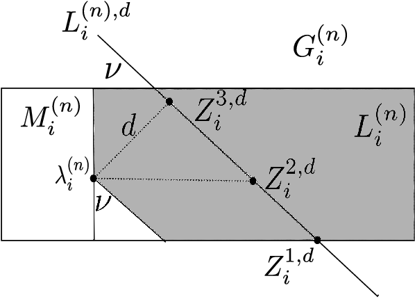
Gi(n):={z∈Mi(n):Re(z)≥Re(λi(n))},i=0,1,\displaystyle G^{(n)}_{i}:=\left\{z\in M^{(n)}_{i}:\operatorname{Re}(z)\geq\operatorname{Re}(\lambda^{(n)}_{i})\right\},\quad i=0,1, (4.25)

and for d≥0d\geq 0

Li(n),d:={λi(n)+e−θ(x+id):x∈ℝ},i=0,1.\displaystyle L^{(n),d}_{i}:=\left\{\lambda^{(n)}_{i}+e^{-\theta}(x+id):x\in\mathbb{R}\right\},\quad i=0,1. (4.26)

Furthermore, we define

L(n)i:=⋃d≥0L(n),di∩G(n)i,i=0,1.\displaystyle L^{(n)}_{i}:=\bigcup_{d\geq 0}L^{(n),d}_{i}\cap G^{(n)}_{i},\quad i=0,1. (4.27)
Refer to caption
Figure 2: Subsets of Mi(n)M_{i}^{(n)}

Note that, by construction, we have

dist(Li(n),d,λi(n))=e−Re⁡θd,i=0,1,\displaystyle\text{dist}\left(L^{(n),d}_{i},\lambda^{(n)}_{i}\right)=e^{-\operatorname{Re}\theta}d,\quad i=0,1, (4.28)

and, by definition of the sets Mi(n)M^{(n)}_{i} and 𝒮\mathcal{S}, it follows that

|z−λi(n)|≤|z−λi(n)−e−θ​s|,∀z∈Mi(n)∖Li(n),∀s∈[ρn+1,∞),\displaystyle\left|z-\lambda^{(n)}_{i}\right|\leq\left|z-\lambda^{(n)}_{i}-e^{-\theta}s\right|,\qquad\forall z\in M^{(n)}_{i}\setminus L^{(n)}_{i},\quad\forall s\in[\rho_{n+1},\infty), (4.29)

where we have used the factor 25\frac{2}{5} in the definition of Mi(n)M^{(n)}_{i}. Let Zi1,dZ^{1,d}_{i} and Zi2,dZ^{2,d}_{i} be the intersections of Li(n),dL^{(n),d}_{i} with the lines

λi(n)−i​25​ρn+1​sin⁡(ν)+ℝandλi(n)+ℝ,\displaystyle\lambda^{(n)}_{i}-i\frac{2}{5}\rho_{n+1}\sin(\nu)+\mathbb{R}\quad\text{and}\quad\lambda^{(n)}_{i}+\mathbb{R}, (4.30)

respectively. Furthermore, we define Zi3,d:=λi(n)+d​ei​π2−θZ^{3,d}_{i}:=\lambda^{(n)}_{i}+de^{i\frac{\pi}{2}-\theta} and recall that ν<π/16\nu<\pi/16. Then, we obtain

supz∈Li(n),d∩Gi(n)|z−λi(n)|2=|Zi1,d−λi(n)|2=e−2​Re⁡θ​d2+|Zi3,d−Zi1,d|2\displaystyle\sup_{z\in L^{(n),d}_{i}\cap G^{(n)}_{i}}\left|z-\lambda^{(n)}_{i}\right|^{2}=\left|Z^{1,d}_{i}-\lambda^{(n)}_{i}\right|^{2}=e^{-2\operatorname{Re}\theta}d^{2}+\left|Z^{3,d}_{i}-Z^{1,d}_{i}\right|^{2}
=e−2​Re⁡θ​d2+(|Zi3,d−Zi2,d|+|Zi2,d−Zi1,d|)2=e−2​Re⁡θ​d2+(e−Re⁡θ​dtan⁡(ν)+25​ρn+1)2.\displaystyle=e^{-2\operatorname{Re}\theta}d^{2}+\left(\left|Z^{3,d}_{i}-Z^{2,d}_{i}\right|+\left|Z^{2,d}_{i}-Z^{1,d}_{i}\right|\right)^{2}=e^{-2\operatorname{Re}\theta}d^{2}+\left(\frac{e^{-\operatorname{Re}\theta}d}{\tan(\nu)}+\frac{2}{5}\rho_{n+1}\right)^{2}. (4.31)

This yields the bound

|z−λi(n)||z−λi(n)−e−θ​s|\displaystyle\frac{\left|z-\lambda^{(n)}_{i}\right|}{\left|z-\lambda^{(n)}_{i}-e^{-\theta}s\right|}
≤[e−2​Re⁡θ​d2|z−λi(n)−e−θ​s|2+(e−Re⁡θ​dtan⁡(ν)​|z−λi(n)−e−θ​s|+2​ρn+15​|z−λi(n)−e−θ​s|)2]12\displaystyle\leq\left[\frac{e^{-2\operatorname{Re}\theta}d^{2}}{\left|z-\lambda^{(n)}_{i}-e^{-\theta}s\right|^{2}}+\left(\frac{e^{-\operatorname{Re}\theta}d}{\tan(\nu)\left|z-\lambda^{(n)}_{i}-e^{-\theta}s\right|}+\frac{2\rho_{n+1}}{5\left|z-\lambda^{(n)}_{i}-e^{-\theta}s\right|}\right)^{2}\right]^{\frac{1}{2}} (4.32)

for s∈[ρn+1,∞)s\in[\rho_{n+1},\infty) and z∈Li(n),d∩Gi(n)z\in L^{(n),d}_{i}\cap G^{(n)}_{i}. Note that |z−λi(n)−e−θ​s|≥e−Re⁡θ​d\left|z-\lambda^{(n)}_{i}-e^{-\theta}s\right|\geq e^{-\operatorname{Re}\theta}d for all z∈Li(n),dz\in L^{(n),d}_{i} and together with (4.24) we obtain

|z−λi(n)||z−λi(n)−e−θ​s|≤[1+(cos⁡(ν)sin⁡(ν)+85​sin⁡(ν))2]12≤4sin⁡(𝝂),\displaystyle\frac{\left|z-\lambda^{(n)}_{i}\right|}{\left|z-\lambda^{(n)}_{i}-e^{-\theta}s\right|}\leq\left[1+\left(\frac{\cos(\nu)}{\sin(\nu)}+\frac{8}{5\sin(\nu)}\right)^{2}\right]^{\frac{1}{2}}\leq\frac{4}{\sin(\boldsymbol{\nu})}, (4.33)

for all z∈Li(n)∩Gi(n)z\in L^{(n)}_{i}\cap G^{(n)}_{i}. This and (4.29) guarantees

1|z−λi(n)−e−θ​s|≤4sin⁡(𝝂)​1|z−λi(n)|∀z∈Mi(n),∀s∈[ρn+1,∞),i=0,1.\displaystyle\frac{1}{\left|z-\lambda^{(n)}_{i}-e^{-\theta}s\right|}\leq\frac{4}{\sin(\boldsymbol{\nu})}\frac{1}{\left|z-\lambda^{(n)}_{i}\right|}\qquad\forall z\in M^{(n)}_{i},\quad\forall s\in[\rho_{n+1},\infty),\quad i=0,1. (4.34)

Now, if |z−λi(n)|≥ρn+1\left|z-\lambda^{(n)}_{i}\right|\geq\rho_{n+1}, we use (4.34) and compute

1|z−λi(n)−e−θ​s|\displaystyle\frac{1}{\left|z-\lambda^{(n)}_{i}-e^{-\theta}s\right|} ≤4sin⁡(𝝂)​ρn+1+|z−λi(n)||z−λi(n)|​1ρn+1+|z−λi(n)|\displaystyle\leq\frac{4}{\sin(\boldsymbol{\nu})}\frac{\rho_{n+1}+\left|z-\lambda^{(n)}_{i}\right|}{\left|z-\lambda^{(n)}_{i}\right|}\frac{1}{\rho_{n+1}+\left|z-\lambda^{(n)}_{i}\right|}
≤8sin⁡(𝝂)​1ρn+1+|z−λi(n)|,\displaystyle\leq\frac{8}{\sin(\boldsymbol{\nu})}\frac{1}{\rho_{n+1}+\left|z-\lambda^{(n)}_{i}\right|}, (4.35)

and if |z−λi(n)|<ρn+1\left|z-\lambda^{(n)}_{i}\right|<\rho_{n+1}, we use (4.24) and find

1|z−λi(n)−e−θ​s|\displaystyle\frac{1}{\left|z-\lambda^{(n)}_{i}-e^{-\theta}s\right|} ≤4sin⁡(𝝂)​ρn+1+|z−λi(n)|ρn+1​1ρn+1+|z−λi(n)|\displaystyle\leq\frac{4}{\sin(\boldsymbol{\nu})}\frac{\rho_{n+1}+\left|z-\lambda^{(n)}_{i}\right|}{\rho_{n+1}}\frac{1}{\rho_{n+1}+\left|z-\lambda^{(n)}_{i}\right|}
≤8sin⁡(𝝂)​1ρn+1+|z−λi(n)|.\displaystyle\leq\frac{8}{\sin(\boldsymbol{\nu})}\frac{1}{\rho_{n+1}+\left|z-\lambda^{(n)}_{i}\right|}. (4.36)

We conclude from (4.35) and (4.36) that for i=0,1i=0,1

1|z−λi(n)−e−θ​s|≤8sin⁡(𝝂)​1ρn+1+|z−λi(n)|∀z∈Mi(n),∀s∈[ρn+1,∞)\displaystyle\frac{1}{\left|z-\lambda^{(n)}_{i}-e^{-\theta}s\right|}\leq\frac{8}{\sin(\boldsymbol{\nu})}\frac{1}{\rho_{n+1}+\left|z-\lambda^{(n)}_{i}\right|}\qquad\forall z\in M^{(n)}_{i},\quad\forall s\in[\rho_{n+1},\infty) (4.37)

holds true. Eqs. (4.22), (4.23), (4.34), together with Lemma 4.7 and Eq. (4.37) yield

‖1H(n),θ+Hf(n,n+1),θ−z​Pi(n,n+1)¯‖≤24+4​ℂn+1sin⁡(𝝂)​1ρn+1+|z−λi(n)|.\displaystyle\left\lVert\frac{1}{H^{(n),\theta}+H_{f}^{(n,n+1),\theta}-z}\overline{P^{(n,n+1)}_{i}}\right\rVert\leq\frac{24+4\mathbb{C}^{n+1}}{\sin(\boldsymbol{\nu})}\frac{1}{\rho_{n+1}+\left|z-\lambda^{(n)}_{i}\right|}. (4.38)

This completes the proof. ∎

Lemma 4.10.

For all z∈Mi(n)∖{λi(n)}z\in M_{i}^{(n)}\setminus\{\lambda_{i}^{(n)}\}, all 0≤r≤|z−λi(n)|0\leq r\leq\left|z-\lambda_{i}^{(n)}\right| and every i∈{0,1}i\in\{0,1\}:

‖Hf(n,n+1)+rHf(n,n+1),θ−(z−λi(n))‖≤10sin⁡(𝝂).\displaystyle\left\lVert\frac{H_{f}^{(n,n+1)}+r}{H_{f}^{(n,n+1),\theta}-\left(z-\lambda_{i}^{(n)}\right)}\right\rVert\leq\frac{10}{\sin(\boldsymbol{\nu})}. (4.39)
Proof.

We calculate:

‖Hf(n,n+1)+rHf(n,n+1),θ−(z−λi(n))‖=supy∈{0}∪[ρn+1,∞)|y+re−θ​y+λi(n)−z|\displaystyle\left\lVert\frac{H_{f}^{(n,n+1)}+r}{H_{f}^{(n,n+1),\theta}-(z-\lambda_{i}^{(n)})}\right\rVert=\sup_{y\in\{0\}\cup[\rho_{n+1},\infty)}\left|\frac{y+r}{e^{-\theta}y+\lambda_{i}^{(n)}-z}\right|
≤|eθ|+|eθ|​supy∈{0}∪[ρn+1,∞)|e−θ​r−λi(n)+ze−θ​y+λi(n)−z|≤|eθ|+(1+|eθ|)​supy∈{0}∪[ρn+1,∞)|z−λi(n)||e−θ​y+λi(n)−z|\displaystyle\leq|e^{\theta}|+|e^{\theta}|\sup_{y\in\{0\}\cup[\rho_{n+1},\infty)}\left|\frac{e^{-\theta}r-\lambda_{i}^{(n)}+z}{e^{-\theta}y+\lambda_{i}^{(n)}-z}\right|\leq|e^{\theta}|+(1+|e^{\theta}|)\sup_{y\in\{0\}\cup[\rho_{n+1},\infty)}\frac{\left|z-\lambda_{i}^{(n)}\right|}{\left|e^{-\theta}y+\lambda_{i}^{(n)}-z\right|}
≤|eθ|+4​(1+|eθ|)sin⁡(𝝂)≤10sin⁡(𝝂),\displaystyle\leq|e^{\theta}|+\frac{4(1+|e^{\theta}|)}{\sin(\boldsymbol{\nu})}\leq\frac{10}{\sin(\boldsymbol{\nu})}, (4.40)

where we have used (4.34) in the second last step. ∎

Lemma 4.11.

Suppose that (𝒫​1\mathcal{P}1)-(𝒫​4\mathcal{P}4) hold true for all m∈ℕm\in\mathbb{N} such that m≤nm\leq n. Then,

‖V(n,n+1),θ​1H(n),θ+Hf(n,n+1),θ−z‖≤2500ρsin(𝝂)2​ℂn+1​ρnμ\displaystyle\left\lVert V^{(n,n+1),\theta}\frac{1}{H^{(n),\theta}+H_{f}^{(n,n+1),\theta}-z}\right\rVert\leq\frac{2500}{\rho\sin(\boldsymbol{\nu})^{2}}\mathbb{C}^{n+1}\rho_{n}^{\mu} (4.41)

for all z∈Mi(n)∖{λi(n)}z\in M_{i}^{(n)}\setminus\{\lambda_{i}^{(n)}\} such that |z−λi(n)|≥110​ρn+1​sin⁡(ν)\left|z-\lambda_{i}^{(n)}\right|\geq\frac{1}{10}\rho_{n+1}\sin(\nu) and for all i∈{0,1}i\in\{0,1\}.

Proof.

Set r=|z−λi(n)|≥110​ρn+1​sin⁡(ν)r=\left|z-\lambda_{i}^{(n)}\right|\geq\frac{1}{10}\rho_{n+1}\sin(\nu). We observe that

‖V(n,n+1),θ​1H(n),θ+Hf(n,n+1),θ−z‖≤‖V(n,n+1),θ​1Hf(n,n+1)+r‖​‖Hf(n,n+1)+rHf(n,n+1),θ−(z−λi(n))‖\displaystyle\left\lVert V^{(n,n+1),\theta}\frac{1}{H^{(n),\theta}+H_{f}^{(n,n+1),\theta}-z}\right\rVert\leq\left\lVert V^{(n,n+1),\theta}\frac{1}{H_{f}^{(n,n+1)}+r}\right\rVert\left\lVert\frac{H_{f}^{(n,n+1)}+r}{H_{f}^{(n,n+1),\theta}-(z-\lambda_{i}^{(n)})}\right\rVert
⋅‖(Hf(n,n+1),θ−(z−λi(n)))​1H(n),θ+Hf(n,n+1),θ−z‖.\displaystyle\hskip 125.19194pt\cdot\left\lVert\left(H_{f}^{(n,n+1),\theta}-(z-\lambda_{i}^{(n)})\right)\frac{1}{H^{(n),\theta}+H_{f}^{(n,n+1),\theta}-z}\right\rVert. (4.42)

Lemma 4.10 yields

‖Hf(n,n+1)+rHf(n,n+1),θ−(z−λi(n))‖≤10sin⁡(𝝂),\displaystyle\left\lVert\frac{H_{f}^{(n,n+1)}+r}{H_{f}^{(n,n+1),\theta}-(z-\lambda_{i}^{(n)})}\right\rVert\leq\frac{10}{\sin(\boldsymbol{\nu})}, (4.43)

and furthermore, we obtain from functional calculus that

‖(Hf(n,n+1),θ−(z−λi(n)))​1H(n),θ+Hf(n,n+1),θ−z‖≤supy∈{0}∪[ρn+1,∞)‖e−θ​y+λi(n)−zH(n),θ+e−θ​y−z‖\displaystyle\left\lVert\left(H_{f}^{(n,n+1),\theta}-(z-\lambda_{i}^{(n)})\right)\frac{1}{H^{(n),\theta}+H_{f}^{(n,n+1),\theta}-z}\right\rVert\leq\sup_{y\in\{0\}\cup[\rho_{n+1},\infty)}\left\lVert\frac{e^{-\theta}y+\lambda_{i}^{(n)}-z}{H^{(n),\theta}+e^{-\theta}y-z}\right\rVert
≤‖Pi(n)‖+supy∈{0}∪[ρn+1,∞)‖λi(n)−(z−e−θ​y)H(n),θ−(z−e−θ​y)​Pi(n)¯‖≤3+ℂn+1≤4​ℂn+1.\displaystyle\leq\left\lVert P_{i}^{(n)}\right\rVert+\sup_{y\in\{0\}\cup[\rho_{n+1},\infty)}\left\lVert\frac{\lambda_{i}^{(n)}-(z-e^{-\theta}y)}{H^{(n),\theta}-(z-e^{-\theta}y)}\overline{P_{i}^{(n)}}\right\rVert\leq 3+\mathbb{C}^{n+1}\leq 4\mathbb{C}^{n+1}. (4.44)

In the last step, we use Lemma 4.7 for the first term. For the second term, we utilize Lemma 3.13, Definition 3.14 and induction hypothesis (𝒫​4\mathcal{P}4), together with Lemma 4.7 and the Definition of C\boldsymbol{C} in Definition 4.1 - see Remark 4.4 (notice that 𝑪≥𝟒​𝒄sin⁡(𝝂/2)≥4​C(3.43)sin⁡(𝝂/2)\boldsymbol{C}\geq\frac{\boldsymbol{4c}}{\sin(\boldsymbol{\nu}/2)}\geq\frac{4C_{\eqref{const:resestinAprima}}}{\sin(\boldsymbol{\nu}/2)} and ‖Pi(n)¯‖≤4\|\overline{P^{(n)}_{i}}\|\leq 4).

Using the proofs in Appendix A, we obtain

‖V(n,n+1),θ​1Hf(n,n+1)+r‖\displaystyle\left\lVert V^{(n,n+1),\theta}\frac{1}{H_{f}^{(n,n+1)}+r}\right\rVert
≤1r​(‖an,n+1​(fθ¯)​(Hf(n,n+1)+r)−12‖+‖an,n+1​(fθ)∗​(Hf(n,n+1)+r)−12‖)\displaystyle\leq\frac{1}{\sqrt{r}}\left(\left\lVert a_{n,n+1}(f^{\overline{\theta}})\left(H_{f}^{(n,n+1)}+r\right)^{-\frac{1}{2}}\right\rVert+\left\lVert{a_{n,n+1}(f^{\theta})}^{*}\left(H_{f}^{(n,n+1)}+r\right)^{-\frac{1}{2}}\right\rVert\right)
≤1r​‖fθ‖𝔥(n,n+1)+2r​‖fθ/ω‖𝔥(n,n+1).\displaystyle\leq\frac{1}{r}\left\lVert f^{\theta}\right\rVert_{\mathfrak{h}^{(n,n+1)}}+\frac{2}{\sqrt{r}}\left\lVert f^{\theta}/\sqrt{\omega}\right\rVert_{\mathfrak{h}^{(n,n+1)}}. (4.45)

We estimate

‖fθ‖𝔥(n,n+1)\displaystyle\left\lVert f^{\theta}\right\rVert_{\mathfrak{h}^{(n,n+1)}} =∫ℬρn∖ℬρn+1d3​k​|fθ​(k)|2=|e−θ⁡(1+μ)​|4​π​∫ρn+1ρnd​u​u1+2​μ|e−2​e2​θ​u2Λ2|\displaystyle=\sqrt{\int_{\mathcal{B}_{\rho_{n}}\setminus\mathcal{B}_{\rho_{n+1}}}\mathrm{d}^{3}k\,|f^{\theta}(k)|^{2}}=|e^{-\theta(1+\mu)}|\sqrt{4\pi\int^{\rho_{n}}_{\rho_{n+1}}\mathrm{d}u\,u^{1+2\mu}|e^{-2e^{2\theta}\frac{u^{2}}{\Lambda^{2}}}}|
≤|e−θ⁡(1+μ)|​4​π​ρnμ​ρn,\displaystyle\leq|e^{-\theta(1+\mu)}|\sqrt{4\pi}\rho_{n}^{\mu}\rho_{n}, (4.46)

and similarly,

‖fθ/ω‖𝔥(n,n+1)≤|e−θ⁡(1+μ)|​4​π​ρnμ​ρn12.\displaystyle\left\lVert f^{\theta}/\sqrt{\omega}\right\rVert_{\mathfrak{h}^{(n,n+1)}}\leq|e^{-\theta(1+\mu)}|\sqrt{4\pi}\rho_{n}^{\mu}\rho_{n}^{\frac{1}{2}}. (4.47)

From our choice of rr, it follows that ρnr≤10ρ​sin⁡(ν)\sqrt{\frac{\rho_{n}}{r}}\leq\frac{\sqrt{10}}{\sqrt{\rho\sin(\nu)}} and, consequently, we obtain

‖V(n,n+1),θ​1Hf(n,n+1)+r‖\displaystyle\left\lVert V^{(n,n+1),\theta}\frac{1}{H_{f}^{(n,n+1)}+r}\right\rVert ≤|e−θ⁡(1+μ)|​4​π​(ρnr+2​ρnr)​ρnμ≤|e−θ⁡(1+μ)|​60ρ​sin⁡(𝝂)​ρnμ.\displaystyle\leq|e^{-\theta(1+\mu)}|\sqrt{4\pi}\left(\frac{\rho_{n}}{r}+2\sqrt{\frac{\rho_{n}}{r}}\right)\rho_{n}^{\mu}\leq|e^{-\theta(1+\mu)}|\frac{60}{\rho\sin(\boldsymbol{\nu})}\rho_{n}^{\mu}. (4.48)

Plugging (4.43), (4.44) and (4.48) into (4.42) yields (we recall that μ∈(0,1/2)\mu\in(0,1/2))

‖V(n,n+1),θ​1H(n),θ+Hf(n,n+1),θ−z‖≤2500ρsin(𝝂)2​ℂn+1​ρnμ.\displaystyle\left\lVert V^{(n,n+1),\theta}\frac{1}{H^{(n),\theta}+H_{f}^{(n,n+1),\theta}-z}\right\rVert\leq\frac{2500}{\rho\sin(\boldsymbol{\nu})^{2}}\mathbb{C}^{n+1}\rho_{n}^{\mu}. (4.49)

This completes the proof. ∎

4.3.2 Induction step

In this section, we apply the results from Section 4.3.1 in order to show the induction step, i.e., we assume that (𝒫​1\mathcal{P}1)-(𝒫​4\mathcal{P}4) hold true for all m≤n∈ℕm\leq n\in\mathbb{N}, and prove that (𝒫​1\mathcal{P}1)-(𝒫​4\mathcal{P}4) hold true for n+1n+1. This together with Remark 4.6 completes the proof of Theorem 4.5.

We first employ the estimates of Section 4.3.1 in order to prove Property (𝒫​2\mathcal{P}2) and (𝒫​3\mathcal{P}3). After this, we prove (𝒫​1\mathcal{P}1). Finally, (𝒫​4\mathcal{P}4) follows again from the results of Section 4.3.1 together with the maximum modulus principle.

Proof of (𝒫​2\mathcal{P}2) and (𝒫​3\mathcal{P}3) :

Proposition 4.12.

Suppose that (𝒫​1\mathcal{P}1)-(𝒫​4\mathcal{P}4) hold true for all m∈ℕm\in\mathbb{N} with m≤nm\leq n. Then,

‖1H(n+1),θ−z‖≤168+8​ℂn+1sin⁡(𝝂)​1ρn+1+|z−λi(n)|,\displaystyle\left\lVert\frac{1}{H^{(n+1),\theta}-z}\right\rVert\leq\frac{168+8\mathbb{C}^{n+1}}{\sin(\boldsymbol{\nu})}\frac{1}{\rho_{n+1}+\left|z-\lambda^{(n)}_{i}\right|}, (4.50)

for all z∈Mi(n)∖{λi(n)}z\in M_{i}^{(n)}\setminus\{\lambda_{i}^{(n)}\} (see Definition 4.8) such that |z−λi(n)|≥110​ρn+1​sin⁡(ν)\left|z-\lambda_{i}^{(n)}\right|\geq\frac{1}{10}\rho_{n+1}\sin(\nu) and for all i∈{0,1}i\in\{0,1\}.

Proof.

Let z∈Mi(n)∖{λi(n)}z\in M_{i}^{(n)}\setminus\{\lambda_{i}^{(n)}\} such that |z−λi(n)|≥110​ρn+1​sin⁡(ν)\left|z-\lambda_{i}^{(n)}\right|\geq\frac{1}{10}\rho_{n+1}\sin(\nu) and i∈{0,1}i\in\{0,1\}. Then, it follows from Lemma 4.11 that

‖V(n,n+1),θ​1H(n),θ+Hf(n,n+1),θ−z‖≤2500ρsin(𝝂)2​ℂn+1​ρnμ.\displaystyle\left\lVert V^{(n,n+1),\theta}\frac{1}{H^{(n),\theta}+H_{f}^{(n,n+1),\theta}-z}\right\rVert\leq\frac{2500}{\rho\sin(\boldsymbol{\nu})^{2}}\mathbb{C}^{n+1}\rho_{n}^{\mu}. (4.51)

Our assumption on gg in Definition 4.3 together with (4.51) yield that (notice that Definition 4.2 implies that Cn+1​ρnμ≤1C^{n+1}\rho_{n}^{\mu}\leq 1 and Definition 4.3 implies that g​2500ρsin(ν)2≤12\frac{g2500}{\rho\sin(\boldsymbol{\nu})^{2}}\leq\frac{1}{2}, see also Remark 4.4)

‖g​V(n,n+1),θ​1H(n),θ+Hf(n,n+1),θ−z‖\displaystyle\left\lVert gV^{(n,n+1),\theta}\frac{1}{H^{(n),\theta}+H_{f}^{(n,n+1),\theta}-z}\right\rVert ≤12.\displaystyle\leq\frac{1}{2}. (4.52)

This and Lemma 4.9 imply that

H(n+1),θ−z=(1+g​V(n,n+1),θ​1H(n),θ+Hf(n,n+1),θ−z)​(H(n),θ+Hf(n,n+1),θ−z)\displaystyle H^{(n+1),\theta}-z=\left(1+gV^{(n,n+1),\theta}\frac{1}{H^{(n),\theta}+H_{f}^{(n,n+1),\theta}-z}\right)\left(H^{(n),\theta}+H_{f}^{(n,n+1),\theta}-z\right) (4.53)

is invertible, and we estimate

‖1H(n+1),θ−z‖\displaystyle\left\lVert\frac{1}{H^{(n+1),\theta}-z}\right\rVert ≤2​‖1H(n),θ+Hf(n,n+1),θ−z‖\displaystyle\leq 2\left\lVert\frac{1}{H^{(n),\theta}+H_{f}^{(n,n+1),\theta}-z}\right\rVert
≤2​‖Pi(n,n+1)‖|z−λi(n)|+2​‖1H(n),θ+Hf(n,n+1),θ−z​Pi(n,n+1)¯‖\displaystyle\leq 2\frac{\left\lVert P^{(n,n+1)}_{i}\right\rVert}{\left|z-\lambda^{(n)}_{i}\right|}+2\left\lVert\frac{1}{H^{(n),\theta}+H_{f}^{(n,n+1),\theta}-z}\overline{P^{(n,n+1)}_{i}}\right\rVert
≤2​‖Pi(n)‖|z−λi(n)|+48+8​ℂn+1sin⁡(𝝂)​1ρn+1+|z−λi(n)|,\displaystyle\leq 2\frac{\left\lVert P^{(n)}_{i}\right\rVert}{\left|z-\lambda^{(n)}_{i}\right|}+\frac{48+8\mathbb{C}^{n+1}}{\sin(\boldsymbol{\nu})}\frac{1}{\rho_{n+1}+\left|z-\lambda^{(n)}_{i}\right|}, (4.54)

where we apply Lemma 4.9. Moreover, Lemma 4.7 implies that ‖Pi(n)‖≤3\left\lVert P^{(n)}_{i}\right\rVert\leq 3 and it follows from |z−λi(n)|≥110​ρn+1​sin⁡(ν)\left|z-\lambda_{i}^{(n)}\right|\geq\frac{1}{10}\rho_{n+1}\sin(\nu) that

1|z−λi(n)|≤20sin⁡(𝝂)​1ρn+1+|z−λi(n)|.\displaystyle\frac{1}{\left|z-\lambda^{(n)}_{i}\right|}\leq\frac{20}{\sin(\boldsymbol{\nu})}\frac{1}{\rho_{n+1}+\left|z-\lambda^{(n)}_{i}\right|}. (4.55)

Altogether, we obtain

‖1H(n+1),θ−z‖\displaystyle\left\lVert\frac{1}{H^{(n+1),\theta}-z}\right\rVert ≤168+8​ℂn+1sin⁡(𝝂)​1ρn+1+|z−λi(n)|,\displaystyle\leq\frac{168+8\mathbb{C}^{n+1}}{\sin(\boldsymbol{\nu})}\frac{1}{\rho_{n+1}+\left|z-\lambda^{(n)}_{i}\right|}, (4.56)

and thereby, complete the proof. ∎

Lemma 4.13.

Suppose that (𝒫​1\mathcal{P}1)-(𝒫​4\mathcal{P}4) hold true for all m∈ℕm\in\mathbb{N} with m≤nm\leq n. We define

P^(n+1)i:=−12​π​i∫γ^i(n)dz1H(n+1),θ−z,\displaystyle\hat{P}^{(n+1)}_{i}:=-\frac{1}{2\pi i}\int_{\hat{\gamma}^{(n)}_{i}}\mathrm{d}z\,\frac{1}{H^{(n+1),\theta}-z}, (4.57)

where

γ^i(n):[0,2​π]→ℂ,t↦λi(n)+18​ρn+1​sin⁡(ν)​ei​t.\displaystyle\hat{\gamma}^{(n)}_{i}:[0,2\pi]\to\mathbb{C},\quad t\mapsto\lambda^{(n)}_{i}+\frac{1}{8}\rho_{n+1}\sin(\nu)e^{it}. (4.58)

Then,

‖P^i(n+1)−Pi(n)⊗PΩ(n,n+1)‖≤|g|ρ​ℂ2​(n+1)+2​ρnμ≤|g|ρ​(12)n.\displaystyle\left\lVert\hat{P}^{(n+1)}_{i}-P^{(n)}_{i}\otimes P_{\Omega^{(n,n+1)}}\right\rVert\leq\frac{|g|}{\rho}\mathbb{C}^{2(n+1)+2}\rho^{\mu}_{n}\leq\frac{|g|}{\rho}\left(\frac{1}{2}\right)^{n}. (4.59)

(The last inequality follows from Definition 4.2.)

Proof.

Recall that the definition of Pi(n)P^{(n)}_{i} is introduced in Eq. (4.9). We notice that the function

Bi(n)∖{λi(n)}∋z↦1H(n),θ−z\displaystyle B^{(n)}_{i}\setminus\{\lambda^{(n)}_{i}\}\ni z\mapsto\frac{1}{H^{(n),\theta}-z} (4.60)

is analytic as an operator valued function and the region between γ^i(n)\hat{\gamma}^{(n)}_{i} and γi(n)\gamma^{(n)}_{i} is contained in the domain of (4.60). We obtain from the Cauchy integral theorem that

P(n)i=−12​π​i∫γi(n)dz1H(n),θ−z=−12​π​i∫γ^i(n)dz1H(n),θ−z.\displaystyle P^{(n)}_{i}=-\frac{1}{2\pi i}\int_{\gamma^{(n)}_{i}}\mathrm{d}z\,\frac{1}{H^{(n),\theta}-z}=-\frac{1}{2\pi i}\int_{\hat{\gamma}^{(n)}_{i}}\mathrm{d}z\,\frac{1}{H^{(n),\theta}-z}. (4.61)

As in Remark 3.5, it turns out that (see Remark 1.2)

P(n)i⊗PΩ(n,n+1)=−12​π​i∫γ^i(n)dz1H(n),θ+Hf(n,n+1),θ−z.\displaystyle P^{(n)}_{i}\otimes P_{\Omega^{(n,n+1)}}=-\frac{1}{2\pi i}\int_{\hat{\gamma}^{(n)}_{i}}\mathrm{d}z\,\frac{1}{H^{(n),\theta}+H_{f}^{(n,n+1),\theta}-z}. (4.62)

We calculate

‖P^i(n+1)−Pi(n)⊗PΩ(n,n+1)‖=12​π​‖∫γ^i(n)d​z​1H(n+1),θ−z−1H(n),θ+Hf(n,n+1),θ−z‖\displaystyle\big\|\hat{P}^{(n+1)}_{i}-P^{(n)}_{i}\otimes P_{\Omega^{(n,n+1)}}\big\|=\frac{1}{2\pi}\Big\|\int_{\hat{\gamma}^{(n)}_{i}}\mathrm{d}z\,\frac{1}{H^{(n+1),\theta}-z}-\frac{1}{H^{(n),\theta}+H_{f}^{(n,n+1),\theta}-z}\Big\|
=12​π​‖∫γ^i(n)d​z​1H(n+1),θ−z​g​V(n,n+1),θ​1H(n),θ+Hf(n,n+1),θ−z‖.\displaystyle=\frac{1}{2\pi}\Big\|\int_{\hat{\gamma}^{(n)}_{i}}\mathrm{d}z\,\frac{1}{H^{(n+1),\theta}-z}gV^{(n,n+1),\theta}\frac{1}{H^{(n),\theta}+H_{f}^{(n,n+1),\theta}-z}\Big\|. (4.63)

Furthermore, Lemma 4.11 implies that for zz in the curve γ^i(n)\hat{\gamma}^{(n)}_{i}

‖g​V(n,n+1),θ​1H(n),θ+Hf(n,n+1),θ−z‖≤|g|​2500ρsin(𝝂)2​ℂn+1​ρnμ,\displaystyle\left\lVert gV^{(n,n+1),\theta}\frac{1}{H^{(n),\theta}+H_{f}^{(n,n+1),\theta}-z}\right\rVert\leq|g|\frac{2500}{\rho\sin(\boldsymbol{\nu})^{2}}\mathbb{C}^{n+1}\rho_{n}^{\mu}, (4.64)

and Proposition 4.12 ensures that

‖1H(n+1),θ−z‖\displaystyle\left\lVert\frac{1}{H^{(n+1),\theta}-z}\right\rVert ≤168+8​ℂn+1sin⁡(𝝂)​1ρn+1.\displaystyle\leq\frac{168+8\mathbb{C}^{n+1}}{\sin(\boldsymbol{\nu})}\frac{1}{\rho_{n+1}}. (4.65)

Eqs (4.63)-(4.65) imply

‖P^i(n+1)−Pi(n)⊗PΩ(n,n+1)‖≤|g|​2500ρsin(𝝂)2​ℂn+1​ρnμ​168+8​ℂn+1sin⁡(𝝂)≤|g|​2500ρsin(𝝂)2​ℂ2​n+2​ρnμ​200sin⁡(𝝂),\displaystyle\left\lVert\hat{P}^{(n+1)}_{i}-P^{(n)}_{i}\otimes P_{\Omega^{(n,n+1)}}\right\rVert\leq|g|\frac{2500}{\rho\sin(\boldsymbol{\nu})^{2}}\mathbb{C}^{n+1}\rho_{n}^{\mu}\frac{168+8\mathbb{C}^{n+1}}{\sin(\boldsymbol{\nu})}\leq\frac{|g|2500}{\rho\sin(\boldsymbol{\nu})^{2}}\mathbb{C}^{2n+2}\rho_{n}^{\mu}\frac{200}{\sin(\boldsymbol{\nu})}, (4.66)

which together with the definition of C\boldsymbol{C} in Definitions 4.1 imply the desired result (Definition 4.1 imply that 500 000sin⁡(ν)3≤ℂ2\frac{500\,000}{\sin(\boldsymbol{\nu})^{3}}\leq\mathbb{C}^{2}, see also Remark 4.4). ∎

Proposition 4.14 (Proof of Properties (𝒫​2\mathcal{P}2) and (𝒫​3\mathcal{P}3)).

Suppose that (𝒫​1\mathcal{P}1)-(𝒫​4\mathcal{P}4) hold true for all m∈ℕm\in\mathbb{N} with m≤nm\leq n, then (𝒫​2\mathcal{P}2) and (𝒫​3\mathcal{P}3) hold true for n+1n+1.

Proof.

Lemma 4.13 implies that ‖P^i(n+1)−Pi(n)⊗PΩ(n,n+1)‖<1\left\lVert\hat{P}^{(n+1)}_{i}-P^{(n)}_{i}\otimes P_{\Omega^{(n,n+1)}}\right\rVert<1 (see Definition 4.3 and recall Remark 4.4). From the induction hypothesis it follows that Pi(n)⊗PΩ(n,n+1)P^{(n)}_{i}\otimes P_{\Omega^{(n,n+1)}} is a rank-one projection. Therefore, P^i(n+1)\hat{P}^{(n+1)}_{i} is also a rank-one projection. Proposition 4.12 implies that H(n+1),θH^{(n+1),\theta} has no spectral points in Mi(n)∖D⁡(λi(n),110​ρn+1​sin⁡(ν))M_{i}^{(n)}\setminus D\Big(\lambda_{i}^{(n)},\frac{1}{10}\rho_{n+1}\sin(\nu)\Big). Since the contour of integration for P^i(n+1)\hat{P}^{(n+1)}_{i} is contained in Mi(n)M_{i}^{(n)} and its interior contains D⁡(λi(n),110​ρn+1​sin⁡(ν))D\Big(\lambda_{i}^{(n)},\frac{1}{10}\rho_{n+1}\sin(\nu)\Big), we obtain that there is only one point in Mi(n)M^{(n)}_{i} contained in the spectrum of Hi(n+1)H^{(n+1)}_{i}. This point is the eigenvalue λi(n+1)\lambda^{(n+1)}_{i} that we introduced above. Lemma 4.12 implies that |λi(n+1)−λi(n)|≤110​ρn+1​sin⁡(ν)|\lambda^{(n+1)}_{i}-\lambda^{(n)}_{i}|\leq\frac{1}{10}\rho_{n+1}\sin(\nu). This in turn implies that Bi(n+1)⊂Mi(n)B_{i}^{(n+1)}\subset M_{i}^{(n)}. Then, λi(n+1)\lambda^{(n+1)}_{i} is the only spectral point of Hi(n+1),θH_{i}^{(n+1),\theta} in Bi(n+1)B_{i}^{(n+1)}, which is Property (𝒫​2\mathcal{P}2). A deformation in the integration contour in the definitions of P^i(n+1)\hat{P}^{(n+1)}_{i} and Pi(n+1)P^{(n+1)}_{i} implies that these projections coincide and, therefore, Property (𝒫​3\mathcal{P}3) is a consequence of Lemma 4.13. ∎

Proof of Property (𝒫​1\mathcal{P}1):

Proposition 4.15 (Proof of Property (𝒫​1\mathcal{P}1)).

Suppose that (𝒫​1\mathcal{P}1)-(𝒫​4\mathcal{P}4) hold true for all m∈ℕm\in\mathbb{N} with m≤nm\leq n. Then, we obtain for i=0,1i=0,1 that

|λi(n+1)−λi(n)|≤|g|​ℂ(n+1)+1​ρn1+μ≤|g|​(12)n​ρn\displaystyle\left|\lambda^{(n+1)}_{i}-\lambda^{(n)}_{i}\right|\leq|g|\mathbb{C}^{(n+1)+1}\rho_{n}^{1+\mu}\leq|g|\left(\frac{1}{2}\right)^{n}\rho_{n} (4.67)

holds true. Notice that the last inequality follows from Definition 4.2.

Proof.

In this proof we explicitly emphasize the dependence of Pi(n)P^{(n)}_{i} on θ\theta and write Pi(n)≡Pi(n),θP^{(n)}_{i}\equiv P^{(n),\theta}_{i}. We define Ψi(n),θ:=Pi(n),θ​φi⊗Ω(n+1)\Psi^{(n),\theta}_{i}:=P^{(n),\theta}_{i}\varphi_{i}\otimes\Omega^{(n+1)}, see Remark 1.2. Proposition 4.14, Property 𝒫​3\mathcal{P}3, Definition 3.14 (see Remark 3.11) and the restrictions for gg in Definition 4.3 imply that ‖Ψi(n),θ−φi⊗Ω(n+1)‖≤1102\|\Psi^{(n),\theta}_{i}-\varphi_{i}\otimes\Omega^{(n+1)}\|\leq\frac{1}{10^{2}}. This guarantees that

‖Ψi(n),θ‖≤2and|⟨Ψi(n),θ¯,Pi(n+1),θ​Ψi(n),θ⟩|≥12.\displaystyle\left\lVert\Psi^{(n),\theta}_{i}\right\rVert\leq 2\qquad\text{and}\qquad\Big|\left\langle\Psi^{(n),\overline{\theta}}_{i},P^{(n+1),\theta}_{i}\Psi^{(n),\theta}_{i}\right\rangle\Big|\geq\frac{1}{2}. (4.68)

Notice that in this work we assume that the imaginary part of θ\theta, ν\nu, is positive. Then, strictly speaking, we do not have the right to use the symbol Ψi(n),θ¯:=Pi(n),θ¯​φi⊗Ω(n+1)\Psi^{(n),\overline{\theta}}_{i}:=P^{(n),\overline{\theta}}_{i}\varphi_{i}\otimes\Omega^{(n+1)}. However, the restriction we impose by assuming that ν\nu is not negative is irrelevant. This is assumed only for convenience in order to simplify our notation. Of course, the same results hold true if we take −π/16<ν<−𝝂-\pi/16<\nu<-\boldsymbol{\nu} (we use this fact in the present proof as well as Pi(n),θ¯=(Pi(n),θ)∗P^{(n),\overline{\theta}}_{i}=\big(P^{(n),\theta}_{i}\big)^{*}). Then, we obtain

λi(n+1)\displaystyle\lambda_{i}^{(n+1)} =⟨Ψi(n),θ¯,H(n+1),θ​Pi(n+1),θ​Ψi(n),θ⟩⟨Ψi(n),θ¯,Pi(n+1),θ​Ψi(n),θ⟩=⟨H(n+1),θ¯​Ψi(n),θ¯,Pi(n+1),θ​Ψi(n),θ⟩⟨Ψi(n),θ¯,Pi(n+1),θ​Ψi(n),θ⟩\displaystyle=\frac{\left\langle\Psi^{(n),\overline{\theta}}_{i},H^{(n+1),\theta}P^{(n+1),\theta}_{i}\Psi^{(n),\theta}_{i}\right\rangle}{\left\langle\Psi^{(n),\overline{\theta}}_{i},P^{(n+1),\theta}_{i}\Psi^{(n),\theta}_{i}\right\rangle}=\frac{\left\langle H^{(n+1),\overline{\theta}}\Psi^{(n),\overline{\theta}}_{i},P^{(n+1),\theta}_{i}\Psi^{(n),\theta}_{i}\right\rangle}{\left\langle\Psi^{(n),\overline{\theta}}_{i},P^{(n+1),\theta}_{i}\Psi^{(n),\theta}_{i}\right\rangle}
=λi(n)+g​⟨V(n,n+1),θ¯​Ψi(n),θ¯,Pi(n+1),θ​Ψi(n),θ⟩⟨Ψi(n),θ¯,Pi(n+1),θ​Ψi(n),θ⟩.\displaystyle=\lambda_{i}^{(n)}+g\frac{\left\langle V^{(n,n+1),\overline{\theta}}\Psi^{(n),\overline{\theta}}_{i},P^{(n+1),\theta}_{i}\Psi^{(n),\theta}_{i}\right\rangle}{\left\langle\Psi^{(n),\overline{\theta}}_{i},P^{(n+1),\theta}_{i}\Psi^{(n),\theta}_{i}\right\rangle}. (4.69)

Now we choose z∈ℂz\in\mathbb{C} such that |z−λi(n)|=ρn+1​sin⁡(ν)10|z-\lambda_{i}^{(n)}|=\frac{\rho_{n+1}\sin(\nu)}{10}. We get that

|λi(n+1)−λi(n)|≤2​‖g​V(n,n+1),θ¯​Pi(n),θ¯​φi⊗Ω(n+1)‖​‖Pi(n+1),θ​Ψi(n),θ‖\displaystyle\left|\lambda_{i}^{(n+1)}-\lambda_{i}^{(n)}\right|\leq 2\left\lVert gV^{(n,n+1),\overline{\theta}}P^{(n),\overline{\theta}}_{i}\varphi_{i}\otimes\Omega^{(n+1)}\right\rVert\Big\|P^{(n+1),\theta}_{i}\Psi^{(n),\theta}_{i}\Big\|
≤54​|z−λi(n)|​‖g​V(n,n+1),θ¯​1H(n),θ¯+Hf(n,n+1),θ¯−z‖\displaystyle\leq 54\left|z-\lambda_{i}^{(n)}\right|\left\lVert gV^{(n,n+1),\overline{\theta}}\frac{1}{H^{(n),\overline{\theta}}+H_{f}^{(n,n+1),\overline{\theta}}-z}\right\rVert
≤g​54​ρn+1​sin⁡(ν)10​2500ρsin(𝝂)2​ℂn+1​ρnμ≤|g|​ℂ(n+1)+1​ρn1+μ≤|g|​(12)n​ρn,\displaystyle\leq g54\frac{\rho_{n+1}\sin(\nu)}{10}\frac{2500}{\rho\sin(\boldsymbol{\nu})^{2}}\mathbb{C}^{n+1}\rho_{n}^{\mu}\leq|g|\mathbb{C}^{(n+1)+1}\rho_{n}^{1+\mu}\leq|g|\left(\frac{1}{2}\right)^{n}\rho_{n}, (4.70)

where we use Lemmas 4.11 and 4.7 and the definition of C\boldsymbol{C} in Definition 4.1 (it implies that 54​2500sin⁡(ν)2≤C54\frac{2500}{\sin(\boldsymbol{\nu})^{2}}\leq\boldsymbol{C}, see also Remark 4.4). ∎

Proof of Property (𝒫​4\mathcal{P}4):

Lemma 4.16.

Suppose that (𝒫​1\mathcal{P}1)-(𝒫​4\mathcal{P}4) hold true for all m∈ℕm\in\mathbb{N} with m≤nm\leq n. Then, for i∈{0,1}i\in\{0,1\}:

‖1H(n+1),θ−z​Pi(n+1)¯‖≤3​168+8​ℂn+1sin⁡(𝝂)​1ρn+1+|z−λi(n)|,∀z∈Mi(m),\displaystyle\left\lVert\frac{1}{H^{(n+1),\theta}-z}\overline{P^{(n+1)}_{i}}\right\rVert\leq 3\frac{168+8\mathbb{C}^{n+1}}{\sin(\boldsymbol{\nu})}\frac{1}{\rho_{n+1}+\left|z-\lambda^{(n)}_{i}\right|},\qquad\forall z\in M_{i}^{(m)}, (4.71)

and hence, for all z∈Bi(n+1)z\in B_{i}^{(n+1)} (recall Bi(n+1)⊂Mi(n)B_{i}^{(n+1)}\subset M_{i}^{(n)} from the proof of Proposition 4.14).

Proof.

Let z∈Mi(n)z\in M_{i}^{(n)} such that |z−λi(n)|≥ρn+110​sin⁡(ν)\left|z-\lambda^{(n)}_{i}\right|\geq\frac{\rho_{n+1}}{10}\sin(\nu) and i∈{0,1}i\in\{0,1\}. Then, (4.71) follows from Proposition 4.12 and the fact that ‖Pi(n+1)¯‖≤3\big\|\overline{P^{(n+1)}_{i}}\big\|\leq 3 (see the proof of Lemma 4.7 and Proposition 4.14). Furthermore, we observe that Mi(n)∋z↦1H(n+1),θ−z​Pi(n+1)¯M_{i}^{(n)}\ni z\mapsto\frac{1}{H^{(n+1),\theta}-z}\overline{P^{(n+1)}_{i}} is analytic (see the proof of Proposition 4.14), and hence, (4.71) follows for |z−λi(n)|≤ρn+110​sin⁡(ν)\left|z-\lambda^{(n)}_{i}\right|\leq\frac{\rho_{n+1}}{10}\sin(\nu) from the maximum modulus principle of complex analysis. ∎

Proposition 4.17 (Proof of Property (𝒫​4\mathcal{P}4)).

Suppose that (𝒫​1\mathcal{P}1)-(𝒫​4\mathcal{P}4) hold true for all m∈ℕm\in\mathbb{N} with m≤nm\leq n and take i∈{0,1}i\in\{0,1\}. Then,

‖1H(n+1),θ−z​Pi(n+1)¯‖\displaystyle\left\lVert\frac{1}{H^{(n+1),\theta}-z}\overline{P^{(n+1)}_{i}}\right\rVert ≤4​168+8​ℂn+1|sin⁡(𝝂)|​1ρn+1+|z−λi(n+1)|≤ℂ(n+1)+1ρn+1+|z−λi(n+1)|\displaystyle\leq 4\frac{168+8\mathbb{C}^{n+1}}{|\sin(\boldsymbol{\nu})|}\frac{1}{\rho_{n+1}+\left|z-\lambda^{(n+1)}_{i}\right|}\leq\frac{\mathbb{C}^{(n+1)+1}}{\rho_{n+1}+\left|z-\lambda^{(n+1)}_{i}\right|} (4.72)

for all z∈Bi(n+1)z\in B^{(n+1)}_{i}.

Proof.

Let i∈{0,1}i\in\{0,1\} and z∈Bi(n+1)z\in B^{(n+1)}_{i}. It follows from Proposition 4.16 that

‖1H(n+1),θ−z​Pi(n+1)¯‖\displaystyle\left\lVert\frac{1}{H^{(n+1),\theta}-z}\overline{P^{(n+1)}_{i}}\right\rVert ≤3​168+8​C​(ν)n+1sin⁡(𝝂)​1ρn+1+|z−λi(n)|\displaystyle\leq 3\frac{168+8C(\nu)^{n+1}}{\sin(\boldsymbol{\nu})}\frac{1}{\rho_{n+1}+\left|z-\lambda^{(n)}_{i}\right|} (4.73)

holds true. Lemma 4.12 implies that |λi(n+1)−λi(n)|≤110​ρn+1​sin⁡(ν)≤110​ρn+1|\lambda^{(n+1)}_{i}-\lambda^{(n)}_{i}|\leq\frac{1}{10}\rho_{n+1}\sin(\nu)\leq\frac{1}{10}\rho_{n+1} . Therefore,

1ρn+1+|z−λi(n)|≤109​1ρn+1+|z−λi(n+1)|.\displaystyle\frac{1}{\rho_{n+1}+\left|z-\lambda^{(n)}_{i}\right|}\leq\frac{10}{9}\frac{1}{\rho_{n+1}+\left|z-\lambda^{(n+1)}_{i}\right|}. (4.74)

This together with (4.73) yields

‖1H(n+1),θ−z​Pi(n+1)¯‖\displaystyle\left\lVert\frac{1}{H^{(n+1),\theta}-z}\overline{P^{(n+1)}_{i}}\right\rVert ≤4​168+8​ℂn+1sin⁡(𝝂)​1ρn+1+|z−λi(n+1)|≤ℂ(n+1)+1ρn+1+|z−λi(n+1)|,\displaystyle\leq 4\frac{168+8\mathbb{C}^{n+1}}{\sin(\boldsymbol{\nu})}\frac{1}{\rho_{n+1}+\left|z-\lambda^{(n+1)}_{i}\right|}\leq\frac{\mathbb{C}^{(n+1)+1}}{\rho_{n+1}+\left|z-\lambda^{(n+1)}_{i}\right|}, (4.75)

where in the last line we use the definition of C\boldsymbol{C} in Definition 4.1 (it implies that 4​168+8sin⁡(ν)≤ℂ4\frac{168+8}{\sin(\boldsymbol{\nu})}\leq\mathbb{C}, see also Remark 4.4). ∎

5 Resolvent and spectral estimates

In this section we prove Theorems 2.6, 2.7 and Proposition 2.1. The resolvent and spectral estimates that we provide are essentially different from the ones presented in Section 4 and [5]. The reason is the following: in [5] the construction of the resonance is based in a sequence of infrared cut-off Hamiltonians. As the parameter, nn, of the sequence tends to infinity the cut-off is removed. Each cut-off Hamiltonian has a resonance that is isolated from the rest of the spectrum and they tend to the resonance of the Hamiltonian without cut-off. The delicate point is to estimate spectra of the cut-off Hamiltonians in such a way that these estimates do not require conditions in the coupling constant that depend on nn. This implies a selection of spectral regions to be analyzed at each step nn. In [5] these regions are chosen in neighborhoods of the resonances and far away from the rest of the spectrum, because the interest lies in constructing the resonance of the full Hamiltonian. Here, we need more subtle estimates in regions that are not only close to the resonances but to other parts of the spectrum of the cut-off Hamiltonians. Then, we get resolvent estimates in terms of the distance to the spectrum rather than the distance to the resonance, as it is done in [5]. The regions that we choose are complements of cones with vertexes in neighborhoods of the resonances. Some parts of the cones are closer to the resonances than to the rest of the spectrum and other parts of the cones are closer to other spectral points. This makes our analysis harder than in [5]. Our analysis requires a geometric construction that controls spectra and resolvents outside cones at step nn using the same information for the exterior of cones at step n−1n-1. In Section 5.1 we analyze the infrared cut-off Hamiltonians and prove spectral and resolvent estimates about them (Theorem 5.5). Geometric aspects of the cones are presented in Lemmas 5.1 and 5.3 below. In Lemma 5.2 we give resolvent (and hence spectral) estimates of a Hamiltonian that is obtained by adding to the Hamiltonian at step nn the free energy of step n+1n+1, using the information we have at step nn. From this last Hamiltonian we obtain the Hamiltonian at step n+1n+1 by adding the interacting energy at step n+1n+1, the analysis of this is presented in Lemma 5.4. Theorem 5.5 is a consequence of Lemma 5.4. The study of the full Hamiltonian is carried out in Theorems 5.9 and 5.10 in Section 5.2, using Theorem 5.5, in a similar manner as in Section 5.1. First, we add the full free energy to the Hamiltonian at step nn in Lemma 5.7, and then, we add the full interacting energy, using Lemma 5.8, in Theorems 5.9 and 5.10. These theorems imply Theorems 2.6 and 2.7. The proof of Proposition 2.1 is not difficult and it is presented in Section 5.3.

We start with introducing some notation. In this section we assume that Definitions 4.1, 4.2 and 4.3 hold true. We additionally assume that 𝑪≥𝑫sin(ν/m)−1\boldsymbol{C}\geq\boldsymbol{D}\sin(\nu/m)^{-1}, in order to freely apply Corollary 3.9 and Eq. (3.44). We fix the Hamiltonians (see Remark 1.2)

H~(n),θ:=H0θ+g​V(n),θ,\displaystyle\tilde{H}^{(n),\theta}:=H^{\theta}_{0}+gV^{(n),\theta}, (5.1)

which are densely defined on the Hilbert space ℋ\mathcal{H}. We recall that we already defined

𝔥(n,∞)=L2​(ℬρn)\displaystyle\mathfrak{h}^{(n,\infty)}=L^{2}(\mathcal{B}_{\rho_{n}}) (5.2)

and the corresponding Fock space ℱ⁡[𝔥(n,∞)]\mathcal{F}[\mathfrak{h}^{(n,\infty)}] (it is defined in (1.7)), with vacuum state Ω(n,∞)\Omega^{(n,\infty)}. We identify, as above,

ℋ≡ℋ(n)⊗ℱ⁡[𝔥(n,∞)].\displaystyle\mathcal{H}\equiv\mathcal{H}^{(n)}\otimes\mathcal{F}[\mathfrak{h}^{(n,\infty)}]. (5.3)

We define the free boson energy operator on ℱ⁡[𝔥(n,∞)]\mathcal{F}[\mathfrak{h}^{(n,\infty)}] by restricting the definition in Eq. (1.1) accordingly and denote it by the symbol Hf(n,∞),0≡Hf(n,∞)H_{f}^{(n,\infty),0}\equiv H_{f}^{(n,\infty)}. We set

Hf(n,∞),θ:=e−θ​Hf(n,∞),0.\displaystyle H_{f}^{(n,\infty),\theta}:=e^{-\theta}H_{f}^{(n,\infty),0}. (5.4)

For every function h∈𝔥(n,∞)h\in\mathfrak{h}^{(n,\infty)}, we define the creation and annihilation operators, an,∞​(h)a_{n,\infty}(h) and an,∞∗​(h)a_{n,\infty}^{*}(h), on ℱ⁡[𝔥(n,∞)]\mathcal{F}[\mathfrak{h}^{(n,\infty)}] according to Eq. (1.10). Again, we use the same notation also for h∈𝔥h\in\mathfrak{h} but then understand hh as its restriction to 𝔥(n,n+1)\mathfrak{h}^{(n,n+1)}.

We fix the following operator (defined on 𝒦⊗ℱ⁡[𝔥(n,∞)]\mathcal{K}\otimes\mathcal{F}[\mathfrak{h}^{(n,\infty)}], and hence, on ℋ\mathcal{H} - see Remark 1.2)

V(n,∞),θ:=σ1⊗(an,∞​(fθ¯)+an,∞​(fθ)∗),\displaystyle V^{(n,\infty),\theta}:=\sigma_{1}\otimes\left(a_{n,\infty}(f^{\overline{\theta}})+a_{n,\infty}(f^{\theta})^{*}\right), (5.5)

and further, we obtain (see Remark 1.2):

Hθ=H(n),θ+Hf(n,∞),θ+g​V(n,∞),θ=H~(n),θ+g​V(n,∞),θ.\displaystyle H^{\theta}=H^{(n),\theta}+H^{(n,\infty),\theta}_{f}+gV^{(n,\infty),\theta}=\tilde{H}^{(n),\theta}+gV^{(n,\infty),\theta}. (5.6)

5.1 Resolvent and spectral estimates multi-scale analysis

In this section we analyze the infrared cut-off Hamiltonians and prove spectral and resolvent estimates about them (Theorem 5.5). Geometric aspects of the cones are presented in Lemmas 5.1 and 5.3 below. In Lemma 5.2 we give resolvent (and hence spectral) estimates of a Hamiltonian that is obtained by adding to the Hamiltonian at step nn the free energy of step n+1n+1, using the information we have at step nn. From this last Hamiltonian we obtain the Hamiltonian at step n+1n+1 by adding the interacting energy at step n+1n+1, the analysis of this is presented in Lemma 5.4. Theorem 5.5 is a consequence of Lemma 5.4.

Lemma 5.1.

Suppose that |g|≤ρ​110​sin⁡(ν/2​m)|g|\leq\rho\frac{1}{10}\sin(\nu/2m). We define for i=0,1i=0,1

qi(n):=λi(n)+14​ρn​e−i​ν,qi(n,n+1):=λi(n)+(25−1100)​ρn+1​e−i​ν.\displaystyle q^{(n)}_{i}:=\lambda^{(n)}_{i}+\frac{1}{4}\rho_{n}e^{-i\nu},\hskip 28.45274ptq^{(n,n+1)}_{i}:=\lambda^{(n)}_{i}+\Big(\frac{2}{5}-\frac{1}{100}\Big)\rho_{n+1}e^{-i\nu}. (5.7)

It follows that

|λi−λi(n)|≤\displaystyle|\lambda_{i}-\lambda_{i}^{(n)}|\leq 2​|g|​ρn1+μ/2\displaystyle 2|g|\rho_{n}^{1+\mu/2} (5.8)

and

𝒞m​(qi(n))⊂𝒞m​(qi(n,n+1))⊂𝒞m​(qi(n+1)),\displaystyle\mathcal{C}_{m}(q^{(n)}_{i})\subset\mathcal{C}_{m}(q^{(n,n+1)}_{i})\subset\mathcal{C}_{m}(q^{(n+1)}_{i}), (5.9)

where the set 𝒞m​(⋅)\mathcal{C}_{m}(\cdot) is defined in (2.7) (see Figure 3). Moreover,

dist⁡(𝒞m​(qi(n,n+1)),ℂ∖𝒞m​(qi(n+1)))≥sin⁡(ν/2​m)​110​ρn+1.\displaystyle{\rm dist}\Big(\mathcal{C}_{m}(q^{(n,n+1)}_{i}),\mathbb{C}\setminus\mathcal{C}_{m}(q^{(n+1)}_{i})\Big)\geq\sin(\nu/2m)\frac{1}{10}\rho_{n+1}. (5.10)

and

dist⁡(𝒞m​(qi(n)),ℂ∖𝒞m​(qi(n,n+1)))≥sin⁡(ν/m)​110​ρn+1.\displaystyle{\rm dist}\Big(\mathcal{C}_{m}(q^{(n)}_{i}),\mathbb{C}\setminus\mathcal{C}_{m}(q^{(n,n+1)}_{i})\Big)\geq\sin(\nu/m)\frac{1}{10}\rho_{n+1}. (5.11)
Refer to caption
Figure 3: Cones
Proof.

That 𝒞m​(qi(n))⊂𝒞m​(qi(n,n+1))\mathcal{C}_{m}(q^{(n)}_{i})\subset\mathcal{C}_{m}(q^{(n,n+1)}_{i}) is immediate. From Theorem 4.5 (Property 𝒫​1\mathcal{P}1) and Definition 4.2 it follows that

|λi(n+1)−λi(n)|≤|g|​(ℂ4​ρ0μ)1/2​((C2​ρμ)n)1/2​ρn1+μ/2≤|g|​12n​ρn1+μ/2.\displaystyle|\lambda_{i}^{(n+1)}-\lambda_{i}^{(n)}|\leq|g|\big(\mathbb{C}^{4}\rho_{0}^{\mu}\big)^{1/2}\Big(\mathbb{(}C^{2}\rho^{\mu})^{n}\Big)^{1/2}\rho_{n}^{1+\mu/2}\leq|g|\frac{1}{2^{n}}\rho_{n}^{1+\mu/2}. (5.12)

This and a geometric series argument prove (5.8). We write

qi(n,n+1)=qi(n+1)+ξ1​e−i​ν+ξ2​i​e−i​ν.\displaystyle q_{i}^{(n,n+1)}=q_{i}^{(n+1)}+\xi_{1}e^{-i\nu}+\xi_{2}ie^{-i\nu}. (5.13)

Eq. (5.12) implies that

|ξ2|≤|g|​ρn,ξ1≥(25−1100−14)​ρn+1−|g|​ρn>110​ρn+1.\displaystyle|\xi_{2}|\leq|g|\rho_{n},\hskip 56.9055pt\xi_{1}\geq\Big(\frac{2}{5}-\frac{1}{100}-\frac{1}{4}\Big)\rho_{n+1}-|g|\rho_{n}>\frac{1}{10}\rho_{n+1}. (5.14)

The last step follows for g>0g>0 sufficiently small (see Definition 4.3). To prove that 𝒞m​(qi(n,n+1))⊂𝒞m​(qi(n+1))\mathcal{C}_{m}(q^{(n,n+1)}_{i})\subset\mathcal{C}_{m}(q^{(n+1)}_{i}), it is enough to show that qi(n,n+1)∈𝒞m​(qi(n+1))q^{(n,n+1)}_{i}\in\mathcal{C}_{m}(q^{(n+1)}_{i}). We shall prove that

|ξ2|/ξ1<tan⁡(ν/2​m),\displaystyle|\xi_{2}|/\xi_{1}<\tan(\nu/2m), (5.15)

which holds true if |g|≤ρ​110​sin⁡(ν/2​m)≤ρ​110​tan⁡(ν/2​m)|g|\leq\rho\frac{1}{10}\sin(\nu/2m)\leq\rho\frac{1}{10}\tan(\nu/2m).

Eq. (5.11) is is implied by the particular geometry considered here because both cones have the same axis, see also Definition 4.2.

Eq. (5.15) implies that the angle between the axis of the cone 𝒞m​(qi(n+1))\mathcal{C}_{m}(q^{(n+1)}_{i}) and the complex number qi(n,n+1)−qi(n+1)q_{i}^{(n,n+1)}-q_{i}^{(n+1)} is smaller than ν/2​m\nu/2m and, therefore, the angle between this complex number and the closest edge of the cone must be larger than ν/2​m\nu/2m. Then, the distance between the referred complex number and the edge is larger than

|qi(n,n+1)−qi(n+1)|​sin⁡(ν/2​m)≥ξ1​sin⁡(ν/2​m)≥sin⁡(ν/2​m)​110​ρn+1,|q_{i}^{(n,n+1)}-q_{i}^{(n+1)}|\sin(\nu/2m)\geq\xi_{1}\sin(\nu/2m)\geq\sin(\nu/2m)\frac{1}{10}\rho_{n+1},

this implies (5.10). ∎

Lemma 5.2.

Assume that for all z∈Bi(1)∖𝒞m​(qi(n))z\in B^{(1)}_{i}\setminus\mathcal{C}_{m}(q_{i}^{(n)})

‖1H(n),θ−z​Pi(n)¯‖≤𝑪n+1​1dist⁡(z,𝒞m​(qi(n))),\displaystyle\Big\|\frac{1}{H^{(n),\theta}-z}\overline{P^{(n)}_{i}}\Big\|\leq\boldsymbol{C}^{n+1}\frac{1}{\rm dist\Big(z,\mathcal{C}_{m}(q_{i}^{(n)})\Big)}, (5.16)

then

‖1H(n),θ+Hf(n,n+1),θ−z​Pi(n,n+1)¯‖≤4​𝑪n+1​1dist⁡(z,𝒞m​(qi(n,n+1))),\displaystyle\Big\|\frac{1}{H^{(n),\theta}+H_{f}^{(n,n+1),\theta}-z}\overline{P^{(n,n+1)}_{i}}\Big\|\leq 4\boldsymbol{C}^{n+1}\frac{1}{\rm dist\Big(z,\mathcal{C}_{m}(q_{i}^{(n,n+1)})\Big)}, (5.17)

and

‖1H(n),θ+Hf(n,n+1),θ−z​Hf(n,n+1)​Pi(n,n+1)¯‖≤100sin⁡(ν/m)​𝑪n+1,\displaystyle\Big\|\frac{1}{H^{(n),\theta}+H_{f}^{(n,n+1),\theta}-z}H_{f}^{(n,n+1)}\overline{P^{(n,n+1)}_{i}}\Big\|\leq\frac{100}{\sin(\nu/m)}\boldsymbol{C}^{n+1}, (5.18)

for all z∈Bi(1)∖𝒞m​(qi(n,n+1))z\in B^{(1)}_{i}\setminus\mathcal{C}_{m}(q_{i}^{(n,n+1)}).

Proof.

Take z∈Bi(1)∖𝒞m​(qi(n,n+1))z\in B^{(1)}_{i}\setminus\mathcal{C}_{m}(q_{i}^{(n,n+1)}). We use the spectral theorem and that (see (4.21))

Pi(n)¯+Pi(n)⊗PΩ(n,n+1)¯=Pi(n,n+1)¯,\displaystyle\overline{P^{(n)}_{i}}+P^{(n)}_{i}\otimes\overline{P_{\Omega^{(n,n+1)}}}=\overline{P^{(n,n+1)}_{i}}, (5.19)

to calculate

‖1H(n),θ+Hf(n,n+1),θ−z​Pi(n,n+1)¯‖\displaystyle\left\lVert\frac{1}{H^{(n),\theta}+H_{f}^{(n,n+1),\theta}-z}\overline{P^{(n,n+1)}_{i}}\right\rVert
≤‖1H(n),θ+Hf(n,n+1),θ−z​Pi(n)¯‖+‖1H(n),θ+Hf(n,n+1),θ−z​Pi(n)⊗PΩ(n,n+1)¯‖\displaystyle\leq\left\lVert\frac{1}{H^{(n),\theta}+H_{f}^{(n,n+1),\theta}-z}\overline{P^{(n)}_{i}}\right\rVert+\left\lVert\frac{1}{H^{(n),\theta}+H_{f}^{(n,n+1),\theta}-z}P^{(n)}_{i}\otimes\overline{P_{\Omega^{(n,n+1)}}}\right\rVert
=sups∈{0}∪[ρn+1,∞)‖1H(n),θ−(z−e−θ​s)​Pi(n)¯‖+sups∈[ρn+1,∞)‖Pi(n)‖|λi(n)−(z−e−θ​s)|.\displaystyle=\sup_{s\in\{0\}\cup[\rho_{n+1},\infty)}\left\lVert\frac{1}{H^{(n),\theta}-(z-e^{-\theta}s)}\overline{P^{(n)}_{i}}\right\rVert+\sup_{s\in[\rho_{n+1},\infty)}\frac{\left\lVert P^{(n)}_{i}\right\rVert}{|\lambda^{(n)}_{i}-(z-e^{-\theta}s)|}. (5.20)

Thanks to the geometry, for all s≥0s\geq 0, we have

dist⁡(z−e−θ​s,𝒞m​(qi(n)))≥dist⁡(z,𝒞m​(qi(n)))≥dist⁡(z,𝒞m​(qi(n,n+1))).\displaystyle{\rm dist}\Big(z-e^{-\theta}s,\mathcal{C}_{m}(q_{i}^{(n)})\Big)\geq{\rm dist}\Big(z,\mathcal{C}_{m}(q_{i}^{(n)})\Big)\geq{\rm dist}\Big(z,\mathcal{C}_{m}(q_{i}^{(n,n+1)})\Big). (5.21)

Eq. (5.21), our hypothesis, Lemma 3.13 and Definitions 3.14 and 4.1 imply that for s≥0s\geq 0

‖1H(n),θ−(z−e−θ​s)​Pi(n)¯‖≤𝑪n+1​1dist⁡(z,𝒞m​(qi(n,n+1))).\displaystyle\left\lVert\frac{1}{H^{(n),\theta}-(z-e^{-\theta}s)}\overline{P^{(n)}_{i}}\right\rVert\leq\boldsymbol{C}^{n+1}\frac{1}{\rm dist\Big(z,\mathcal{C}_{m}(q_{i}^{(n,n+1)})\Big)}. (5.22)

Notice that for s≥ρn+1s\geq\rho_{n+1},

z−e−θ​s∉𝒞m​(λi(n))\displaystyle z-e^{-\theta}s\notin\mathcal{C}_{m}(\lambda_{i}^{(n)}) (5.23)

and, therefore,

|λi(n)−(z−e−θ​s)|≥dist⁡(z−e−θ​s,𝒞m​(λi(n)))=\displaystyle|\lambda^{(n)}_{i}-(z-e^{-\theta}s)|\geq{\rm dist}\Big(z-e^{-\theta}s,\mathcal{C}_{m}(\lambda_{i}^{(n)})\Big)= dist⁡(z,𝒞m​(λi(n)+e−θ​s))\displaystyle{\rm dist}\Big(z,\mathcal{C}_{m}(\lambda_{i}^{(n)}+e^{-\theta}s)\Big) (5.24)
≥\displaystyle\geq dist⁡(z,𝒞m​(qi(n,n+1))).\displaystyle{\rm dist}\Big(z,\mathcal{C}_{m}(q_{i}^{(n,n+1)})\Big).

Eqs. (5.21), (5.22) and (5.24), and Lemma 4.7 together with Definition 4.1 imply Eq. (5.17).

Now, we prove Eq. (5.18). As in (5.20) and (5.22), we have

‖1H(n),θ+Hf(n,n+1),θ−z​Hf(n,n+1)​Pi(n,n+1)¯‖\displaystyle\left\lVert\frac{1}{H^{(n),\theta}+H_{f}^{(n,n+1),\theta}-z}H_{f}^{(n,n+1)}\overline{P^{(n,n+1)}_{i}}\right\rVert
≤sups∈{0}∪[ρn+1,∞)𝑪n+1​sdist⁡(z−e−θ​s,𝒞m​(qi(n,n+1)))+sups∈[ρn+1,∞)‖Pi(n)‖​s|λi(n)−(z−e−θ​s)|.\displaystyle\hskip 14.22636pt\leq\sup_{s\in\{0\}\cup[\rho_{n+1},\infty)}\boldsymbol{C}^{n+1}\frac{s}{{\rm dist}\Big(z-e^{-\theta}s,\mathcal{C}_{m}(q_{i}^{(n,n+1)})\Big)}+\sup_{s\in[\rho_{n+1},\infty)}\frac{\left\lVert P^{(n)}_{i}\right\rVert s}{|\lambda^{(n)}_{i}-(z-e^{-\theta}s)|}. (5.25)

Notice that for z∉𝒞m​(qi(n,n+1)),z\notin\mathcal{C}_{m}(q_{i}^{(n,n+1)}),

dist⁡(z−e−θ​s,𝒞m​(qi(n,n+1)))≥12​s​sin⁡(ν/m).\displaystyle{\rm dist}\Big(z-e^{-\theta}s,\mathcal{C}_{m}(q_{i}^{(n,n+1)})\Big)\geq\frac{1}{2}s\sin(\nu/m). (5.26)

Now we argue as in (5.24) and obtain, for s≥ρn+1s\geq\rho_{n+1},

|λi(n)−(z−e−θ​s)|≥dist⁡(z−e−θ​s,𝒞m​(λi(n)))=\displaystyle|\lambda^{(n)}_{i}-(z-e^{-\theta}s)|\geq{\rm dist}\Big(z-e^{-\theta}s,\mathcal{C}_{m}(\lambda_{i}^{(n)})\Big)= dist⁡(z−110​e−θ​s,𝒞m​(λi(n)+910​e−θ​s))\displaystyle{\rm dist}\Big(z-\frac{1}{10}e^{-\theta}s,\mathcal{C}_{m}(\lambda_{i}^{(n)}+\frac{9}{10}e^{-\theta}s)\Big) (5.27)
≥\displaystyle\geq dist⁡(z−110​e−θ​s,𝒞m​(qi(n,n+1)))\displaystyle{\rm dist}\Big(z-\frac{1}{10}e^{-\theta}s,\mathcal{C}_{m}(q_{i}^{(n,n+1)})\Big)
≥\displaystyle\geq 120​s​sin⁡(ν/m).\displaystyle\frac{1}{20}s\sin(\nu/m).

Eqs. (5.25), (5.26) and (5.27) together with Lemma 4.7 imply Eq. (5.18). ∎

Lemma 5.3.

Let 𝒞(1),𝒞(2),𝒞(3)\mathcal{C}^{(1)},\mathcal{C}^{(2)},\mathcal{C}^{(3)} be cones in ℂ\mathbb{C}, such that C(1)⫋𝒞(2)⫋𝒞(3)C^{(1)}\subsetneqq\mathcal{C}^{(2)}\subsetneqq\mathcal{C}^{(3)}, of the form (2.7) - with the same mm. Assume that

maxy∈∂𝒞(2)⁡dist⁡(y,𝒞(1))≤12​dist​(ℂ∖𝒞(3),𝒞(1)).\displaystyle\max_{y\in\partial\mathcal{C}^{(2)}}{\rm dist}\Big(y,\mathcal{C}^{(1)}\Big)\leq\frac{1}{2}{\rm dist}\Big(\mathbb{C}\setminus\mathcal{C}^{(3)},\mathcal{C}^{(1)}\Big). (5.28)

Then, for every z∉𝒞(3)z\notin\mathcal{C}^{(3)}:

dist⁡(z,𝒞(2))≥12​dist​(z,𝒞(1)).\displaystyle{\rm dist}\Big(z,\mathcal{C}^{(2)}\Big)\geq\frac{1}{2}{\rm dist}\Big(z,\mathcal{C}^{(1)}\Big). (5.29)
Proof.

We take z∉𝒞(3)z\notin\mathcal{C}^{(3)}, y∈∂𝒞(2)y\in\partial\mathcal{C}^{(2)}, and x∈𝒞(1)x\in\mathcal{C}^{(1)} such that |y−x|=dist⁡(y,𝒞(1))|y-x|={\rm dist}\Big(y,\mathcal{C}^{(1)}\Big). We calculate

|z−y|≥|z−x|−|x−y|\displaystyle|z-y|\geq|z-x|-|x-y| =|z−x|−dist⁡(y,𝒞(1))\displaystyle=|z-x|-{\rm dist}\Big(y,\mathcal{C}^{(1)}\Big) (5.30)
≥|z−x|−12​dist​(ℂ∖𝒞(3),𝒞(1)).\displaystyle\geq|z-x|-\frac{1}{2}{\rm dist}\Big(\mathbb{C}\setminus\mathcal{C}^{(3)},\mathcal{C}^{(1)}\Big). (5.31)

Next, we use that

dist⁡(ℂ∖𝒞(3),𝒞(1))≤|z−x|\displaystyle{\rm dist}\Big(\mathbb{C}\setminus\mathcal{C}^{(3)},\mathcal{C}^{(1)}\Big)\leq|z-x| (5.32)

to obtain:

|z−y|≥12​|z−x|≥12​dist​(z,𝒞(1)),\displaystyle|z-y|\geq\frac{1}{2}|z-x|\geq\frac{1}{2}{\rm dist}\Big(z,\mathcal{C}^{(1)}\Big), (5.33)

and therefore,

dist⁡(z,𝒞(2))≥12​dist​(z,𝒞(1)).\displaystyle{\rm dist}\Big(z,\mathcal{C}^{(2)}\Big)\geq\frac{1}{2}{\rm dist}\Big(z,\mathcal{C}^{(1)}\Big). (5.34)

∎

Lemma 5.4.

Assume that |g|≤sin(ν/2m)3ρ108|g|\leq\frac{\sin(\nu/2m)^{3}\rho}{10^{8}} and ρ≤10−3​sin⁡(ν/m)​e1\rho\leq 10^{-3}\sin(\nu/m)e_{1} and that for all z∈Bi(1)∖𝒞m​(qi(n))z\in B^{(1)}_{i}\setminus\mathcal{C}_{m}(q_{i}^{(n)})

‖1H(n),θ−z​Pi(n)¯‖≤𝑪n+1​1dist⁡(z,𝒞m​(qi(n))),\displaystyle\Big\|\frac{1}{H^{(n),\theta}-z}\overline{P^{(n)}_{i}}\Big\|\leq\boldsymbol{C}^{n+1}\frac{1}{\rm dist\Big(z,\mathcal{C}_{m}(q_{i}^{(n)})\Big)}, (5.35)

then (Bi(1)∖𝒞m​(qi(n+1)))∖{λi(n+1)}\Big(B^{(1)}_{i}\setminus\mathcal{C}_{m}(q_{i}^{(n+1)})\Big)\setminus\{\lambda_{i}^{(n+1)}\} is contained in the resolvent set of H(n+1),θH^{(n+1),\theta} and

‖1H(n+1),θ−z​Pi(n+1)¯‖≤\displaystyle\Big\|\frac{1}{H^{(n+1),\theta}-z}\overline{P_{i}^{(n+1)}}\Big\|\leq 105sin⁡(ν/m)2​𝑪n+1​1dist⁡(z,𝒞m​(qi(n,n+1))).,\displaystyle\frac{10^{5}}{\sin(\nu/m)^{2}}\boldsymbol{C}^{n+1}\frac{1}{\rm dist\Big(z,\mathcal{C}_{m}(q_{i}^{(n,n+1)})\Big).}, (5.36)

for every z∈Bi(1)∖𝒞m​(qi(n+1))z\in B^{(1)}_{i}\setminus\mathcal{C}_{m}(q_{i}^{(n+1)}). Moreover, assuming that 𝐂≥105sin⁡(ν/m)2\boldsymbol{C}\geq\frac{10^{5}}{\sin(\nu/m)^{2}}, for all z∈Bi(1)∖𝒞m​(qi(n+1))z\in B^{(1)}_{i}\setminus\mathcal{C}_{m}(q_{i}^{(n+1)})

‖1H(n+1),θ−z​Pi(n)¯‖≤𝑪n+2​1dist⁡(z,𝒞m​(qi(n+1))).\displaystyle\Big\|\frac{1}{H^{(n+1),\theta}-z}\overline{P^{(n)}_{i}}\Big\|\leq\boldsymbol{C}^{n+2}\frac{1}{\rm dist\Big(z,\mathcal{C}_{m}(q_{i}^{(n+1)})\Big)}. (5.37)
Proof.

Eq. (5.37) is a consequence of (5.36) and (5.9) together with 𝑪≥105sin⁡(ν/m)2\boldsymbol{C}\geq\frac{10^{5}}{\sin(\nu/m)^{2}} . We fix the cones:

𝒞(1)\displaystyle\mathcal{C}^{(1)} =𝒞m​(qi(n,n+1)),𝒞(2)=𝒞m​(qi(n,n+1)−ρn+1​e−i​ν),\displaystyle=\mathcal{C}_{m}(q_{i}^{(n,n+1)}),\hskip 14.22636pt\mathcal{C}^{(2)}=\mathcal{C}_{m}(q_{i}^{(n,n+1)}-\rho_{n+1}e^{-i\nu}),\hskip 14.22636pt (5.38)
𝒞(3)\displaystyle\mathcal{C}^{(3)} =𝒞m​(qi(n,n+1)−2​1sin⁡(ν/m)​ρn+1​e−i​ν).\displaystyle=\mathcal{C}_{m}(q_{i}^{(n,n+1)}-2\frac{1}{\sin(\nu/m)}\rho_{n+1}e^{-i\nu}).

Note that the cones we just defined fulfill the hypothesis of Lemma 5.3. They satisfy the following properties (see Lemma 5.3). For all z∉C(3)z\notin C^{(3)} and for all s≥0s\geq 0:

λi(n)∈𝒞(2),|(z−s​e−θ)−λi(n)|≥dist⁡((z−s​e−θ),𝒞(2))≥dist⁡(z,𝒞(2))≥12​dist​(z,𝒞(1)),\displaystyle\lambda_{i}^{(n)}\in\mathcal{C}^{(2)},\hskip 14.22636pt|(z-se^{-\theta})-\lambda_{i}^{(n)}|\geq{\rm dist}((z-se^{-\theta}),\mathcal{C}^{(2)})\geq{\rm dist}(z,\mathcal{C}^{(2)})\geq\frac{1}{2}{\rm dist}(z,\mathcal{C}^{(1)}), (5.39)

where we use that z−s​e−θ∉C(3)z-se^{-\theta}\notin C^{(3)}. We define z1=x1(1)+i​x2(1)z_{1}=x^{(1)}_{1}+ix^{(1)}_{2} (x1(1),x2(1)∈ℝx^{(1)}_{1},x^{(1)}_{2}\in\mathbb{R}) to be the point in the intersection of qi(n,n+1)+1100​ρn+1​e−i​ν+ℝq_{i}^{(n,n+1)}+\frac{1}{100}\rho_{n+1}e^{-i\nu}+\mathbb{R} with ∂𝒞(1)\partial\mathcal{C}^{(1)} with smaller x1(1)x^{(1)}_{1}, and similarly, z2=x1(2)+i​x2(2)z_{2}=x^{(2)}_{1}+ix^{(2)}_{2} the point in the intersection of qi(n,n+1)+1100​ρn+1​e−i​ν+i​ℝq_{i}^{(n,n+1)}+\frac{1}{100}\rho_{n+1}e^{-i\nu}+i\mathbb{R} with 𝒞(1)\mathcal{C}^{(1)} with bigger x2(2)x^{(2)}_{2} . We recall that

qi(n,n+1)+1100​ρn+1​e−i​ν=λi(n)+25​ρn+1​e−i​ν∈Mi(n),\displaystyle q_{i}^{(n,n+1)}+\frac{1}{100}\rho_{n+1}e^{-i\nu}=\lambda_{i}^{(n)}+\frac{2}{5}\rho_{n+1}e^{-i\nu}\in M^{(n)}_{i}, (5.40)

see Definition 4.8, and therefore,

z1,z2∈Mi(n)\displaystyle z_{1},z_{2}\in M^{(n)}_{i} (5.41)

(the factor 1100\frac{1}{100} is chosen for this reason). Now, we set

𝒰:=(𝒞(3)∖𝒞(1)¯)∩⋃t∈[0,1]{t​z1+(1−t)​z2+e−i​ν​ℝ}.\displaystyle\mathcal{U}:=\Big(\overline{\mathcal{C}^{(3)}\setminus\mathcal{C}^{(1)}}\Big)\cap\bigcup_{t\in[0,1]}\big\{tz_{1}+(1-t)z_{2}+e^{-i\nu}\mathbb{R}\big\}. (5.42)

Our restrictions on ρ\rho together with (5.40) and (5.41) imply that

𝒰⊂Mi(n).\displaystyle\mathcal{U}\subset M^{(n)}_{i}. (5.43)

It follow from the particular considered geometry at hand that the distance between the boundary of 𝒰\mathcal{U} and λi(n)\lambda_{i}^{(n)} is bigger or equal than the distance between the point z2z_{2} and the line qi(n,n+1)+ℝ​e−i​νq_{i}^{(n,n+1)}+\mathbb{R}e^{-i\nu}, which equals tan⁡(ν/m)​ι\tan(\nu/m)\iota, where ι\iota is the distance between qi(n,n+1)q_{i}^{(n,n+1)} and the intersection of the line z2+i​e−i​ν​ℝz_{2}+ie^{-i\nu}\mathbb{R} with qi(n,n+1)+ℝ​e−i​νq_{i}^{(n,n+1)}+\mathbb{R}e^{-i\nu}. Then ι\iota is bigger or equal to the distance between qi(n,n+1)q_{i}^{(n,n+1)} and the intersection of the line z~2+i​e−i​ν​ℝ\tilde{z}_{2}+ie^{-i\nu}\mathbb{R} with qi(n,n+1)+ℝ​e−i​νq_{i}^{(n,n+1)}+\mathbb{R}e^{-i\nu}, where z~2\tilde{z}_{2} is the intersection of z2+i​ℝz_{2}+i\mathbb{R} with qi(n,n+1)+ℝq_{i}^{(n,n+1)}+\mathbb{R}. Then, ι≥1100​ρn+1​cos⁡(ν)​cos⁡(ν)\iota\geq\frac{1}{100}\rho_{n+1}\cos(\nu)\cos(\nu). We obtain that

dist⁡(∂𝒰,λi(n))≥1100​ρn+1​cos⁡(ν)​cos⁡(ν)​tan⁡(ν/m)≥1200​sin⁡(ν/m)​ρn+1,\displaystyle{\rm dist}(\partial\mathcal{U},\lambda_{i}^{(n)})\geq\frac{1}{100}\rho_{n+1}\cos(\nu)\cos(\nu)\tan(\nu/m)\geq\frac{1}{200}\sin(\nu/m)\rho_{n+1}, (5.44)

where we use that θ∈𝒮\theta\in\mathcal{S}.

For every z∈𝒞(3)∖𝒞(1)∖𝒰¯z\in\overline{\mathcal{C}^{(3)}\setminus\mathcal{C}^{(1)}\setminus\mathcal{U}} and s≥0s\geq 0, we have that

|λi(n)−(z−s​e−θ)|≥1200​sin⁡(ν/m)​ρn+1\displaystyle|\lambda_{i}^{(n)}-(z-se^{-\theta})|\geq\frac{1}{200}\sin(\nu/m)\rho_{n+1} (5.45)

and

dist⁡(z,𝒞(1))≤2​1sin⁡(ν/m)​ρn+1.{\rm dist}(z,\mathcal{C}^{(1)})\leq 2\frac{1}{\sin(\nu/m)}\rho_{n+1}. (5.46)

It follows form (5.45), (5.46) together with (5.39) that

dist⁡(z,𝒞(1))|λi(n)−(z−s​e−θ)|≤400​1sin⁡(ν/m)2,\displaystyle\frac{{\rm dist}(z,\mathcal{C}^{(1)})}{|\lambda_{i}^{(n)}-(z-se^{-\theta})|}\leq 400\frac{1}{\sin(\nu/m)^{2}}, (5.47)

for every z∈(Bi(1)∖𝒞(1))∖𝒰z\in\Big(B_{i}^{(1)}\setminus\mathcal{C}^{(1)}\Big)\setminus\mathcal{U}. This implies, we also use Lemma 5.2 and the spectral theorem that (actually we only need s=0s=0 above),

‖1H(n),θ+Hf(n,n+1),θ−z‖≤104sin⁡(ν/m)2​𝑪n+1​1dist⁡(z,𝒞m​(qi(n,n+1))),\displaystyle\Big\|\frac{1}{H^{(n),\theta}+H_{f}^{(n,n+1),\theta}-z}\Big\|\leq\frac{10^{4}}{\sin(\nu/m)^{2}}\boldsymbol{C}^{n+1}\frac{1}{\rm dist\Big(z,\mathcal{C}_{m}(q_{i}^{(n,n+1)})\Big)}, (5.48)

and for every positive number rr

‖1H(n),θ+Hf(n,n+1),θ−z​(Hf(n,n+1)+r)‖≤\displaystyle\Big\|\frac{1}{H^{(n),\theta}+H_{f}^{(n,n+1),\theta}-z}(H_{f}^{(n,n+1)}+r)\Big\|\leq 100sin⁡(ν/m)​𝑪n+1\displaystyle\frac{100}{\sin(\nu/m)}\boldsymbol{C}^{n+1} (5.49)
+104sin⁡(ν/m)2​𝑪n+1​rdist⁡(z,𝒞m​(qi(n,n+1))),\displaystyle+\frac{10^{4}}{\sin(\nu/m)^{2}}\boldsymbol{C}^{n+1}\frac{r}{\rm dist\Big(z,\mathcal{C}_{m}(q_{i}^{(n,n+1)})\Big)},

where we use that Hf(n,n+1)​Pi(n,n+1)=0H_{f}^{(n,n+1)}P_{i}^{(n,n+1)}=0, for every z∈(Bi(1)∖𝒞(1))∖𝒰z\in\Big(B^{(1)}_{i}\setminus\mathcal{C}^{(1)}\Big)\setminus\mathcal{U}. Choosing r=ρn+1r=\rho_{n+1}, and additionally, z∉𝒞m​(qi(n+1))z\notin\mathcal{C}_{m}(q_{i}^{(n+1)}), we get from (5.10) and (5.49) that

‖1H(n),θ+Hf(n,n+1),θ−z​(Hf(n,n+1)+r)‖≤\displaystyle\Big\|\frac{1}{H^{(n),\theta}+H_{f}^{(n,n+1),\theta}-z}(H_{f}^{(n,n+1)}+r)\Big\|\leq 𝑪n+1​106sin⁡(ν/2​m)3.\displaystyle\boldsymbol{C}^{n+1}\frac{10^{6}}{\sin(\nu/2m)^{3}}. (5.50)

We observe that

‖V(n,n+1),θ​1H(n),θ+Hf(n,n+1),θ−z‖≤‖V(n,n+1),θ​1Hf(n,n+1)+r‖\displaystyle\left\lVert V^{(n,n+1),\theta}\frac{1}{H^{(n),\theta}+H_{f}^{(n,n+1),\theta}-z}\right\rVert\leq\left\lVert V^{(n,n+1),\theta}\frac{1}{H_{f}^{(n,n+1)}+r}\right\rVert
×‖(Hf(n,n+1)+r)​1H(n),θ+Hf(n,n+1),θ−z‖.\displaystyle\hskip 182.09746pt\times\left\lVert\left(H_{f}^{(n,n+1)}+r\right)\frac{1}{H^{(n),\theta}+H_{f}^{(n,n+1),\theta}-z}\right\rVert. (5.51)

Then, we have (see also Eq. (4.48))

‖g​V(n,n+1),θ​1H(n),θ+Hf(n,n+1),θ−z‖≤|g|​106sin⁡(ν/2​m)3​𝑪n+1​‖V(n,n+1),θ​1Hf(n,n+1)+r‖\displaystyle\big\|gV^{(n,n+1),\theta}\frac{1}{H^{(n),\theta}+H_{f}^{(n,n+1),\theta}-z}\Big\|\leq|g|\frac{10^{6}}{\sin(\nu/2m)^{3}}\boldsymbol{C}^{n+1}\left\lVert V^{(n,n+1),\theta}\frac{1}{H_{f}^{(n,n+1)}+r}\right\rVert
≤|g|​106sin⁡(ν/2​m)3​𝑪n+1​|e−θ⁡(1+μ)|​4​π​(ρnr+2​ρnr)​ρnμ≤108​|g|2sin(ν/2m)3ρ​𝑪n+1​ρnμ≤12,\displaystyle\leq|g|\frac{10^{6}}{\sin(\nu/2m)^{3}}\boldsymbol{C}^{n+1}|e^{-\theta(1+\mu)}|\sqrt{4\pi}\left(\frac{\rho_{n}}{r}+2\sqrt{\frac{\rho_{n}}{r}}\right)\rho_{n}^{\mu}\leq\frac{10^{8}|g|}{2\sin(\nu/2m)^{3}\rho}\boldsymbol{C}^{n+1}\rho_{n}^{\mu}\leq\frac{1}{2}, (5.52)

because Definition 4.2 implies that 𝑪n+1​ρnμ≤1\boldsymbol{C}^{n+1}\rho_{n}^{\mu}\leq 1 (we use as well our restrictions in |g||g|).

Eq. (5.52) and a Neumann series argument implies that (Bi(1)∖𝒞m​(qi(n+1)))∖𝒰\Big(B_{i}^{(1)}\setminus\mathcal{C}_{m}(q_{i}^{(n+1)})\Big)\setminus\mathcal{U} is contained in the resolvent set of H(n+1),θH^{(n+1),\theta} and for all zz in this set (see also (5.48))

‖1H(n+1),θ−z‖≤\displaystyle\Big\|\frac{1}{H^{(n+1),\theta}-z}\Big\|\leq 2​104sin⁡(ν/m)2​𝑪n+1​1dist⁡(z,𝒞m​(qi(n,n+1))).\displaystyle 2\frac{10^{4}}{\sin(\nu/m)^{2}}\boldsymbol{C}^{n+1}\frac{1}{\rm dist\Big(z,\mathcal{C}_{m}(q_{i}^{(n,n+1)})\Big)}. (5.53)

Lemma 4.16 ensures that λi(n+1)\lambda^{(n+1)}_{i} is the only spectral point of H(n+1),θH^{(n+1),\theta} in Mi(n)M^{(n)}_{i}. Hence, the function

𝒰∋z↦1H(n+1),θ−z​Pi(n+1)¯\displaystyle\mathcal{U}\ni z\mapsto\frac{1}{H^{(n+1),\theta}-z}\overline{P_{i}^{(n+1)}} (5.54)

is analytic. The maximum modulus principle implies that it attains its maximum on the boundary of 𝒰\mathcal{U}, then we have (see Definition 4.1 and Lemma 4.16)

‖1H(n+1),θ−z​Pi(n+1)¯‖≤\displaystyle\Big\|\frac{1}{H^{(n+1),\theta}-z}\overline{P_{i}^{(n+1)}}\Big\|\leq 𝑪n+1​1ρn+1\displaystyle\boldsymbol{C}^{n+1}\frac{1}{\rho_{n+1}} (5.55)

for every z∈𝒰z\in\mathcal{U}. Next, notice that, for z∈𝒰,z\in\mathcal{U}, dist⁡(z,𝒞m​(qi(n,n+1)))≤2sin⁡(ν/m)​ρn+1{\rm dist}\Big(z,\mathcal{C}_{m}(q_{i}^{(n,n+1)})\Big)\leq\frac{2}{\sin(\nu/m)}\rho_{n+1}. Then, we obtain

‖1H(n+1),θ−z​Pi(n+1)¯‖≤\displaystyle\Big\|\frac{1}{H^{(n+1),\theta}-z}\overline{P_{i}^{(n+1)}}\Big\|\leq 1sin⁡(ν/m)​𝑪n+1​2dist⁡(z,𝒞m​(qi(n,n+1)))\displaystyle\frac{1}{\sin(\nu/m)}\boldsymbol{C}^{n+1}\frac{2}{{\rm dist}\Big(z,\mathcal{C}_{m}(q_{i}^{(n,n+1)})\Big)} (5.56)
≤\displaystyle\leq 1sin⁡(ν/m)​𝑪n+1​2dist⁡(z,𝒞m​(qi(n+1))),\displaystyle\frac{1}{\sin(\nu/m)}\boldsymbol{C}^{n+1}\frac{2}{{\rm dist}\Big(z,\mathcal{C}_{m}(q_{i}^{(n+1)})\Big)},

Eqs. (5.53) and (5.56) together with Lemma 4.7 imply the desired result. ∎

The next theorem is proved inductively using Corollary 3.9 and Lemma 5.4. This is the main theorem of the present subsection.

Theorem 5.5.

Assume that |g|≤sin(ν/2m)3ρ108|g|\leq\frac{\sin(\nu/2m)^{3}\rho}{10^{8}}, ρ≤10−3​sin⁡(ν/m)​e1\rho\leq 10^{-3}\sin(\nu/m)e_{1} and 𝐂≥105sin⁡(ν/m)2\boldsymbol{C}\geq\frac{10^{5}}{\sin(\nu/m)^{2}}. Then, for all n∈ℕn\in\mathbb{N} and for all z∈Bi(1)∖𝒞m​(qi(n))z\in B^{(1)}_{i}\setminus\mathcal{C}_{m}(q_{i}^{(n)}):

‖1H(n),θ−z​Pi(n)¯‖≤𝑪n+1​1dist⁡(z,𝒞m​(qi(n))).\displaystyle\Big\|\frac{1}{H^{(n),\theta}-z}\overline{P^{(n)}_{i}}\Big\|\leq\boldsymbol{C}^{n+1}\frac{1}{\rm dist\Big(z,\mathcal{C}_{m}(q_{i}^{(n)})\Big)}. (5.57)

5.2 Resolvent estimates

In this section we study the spectrum and resolvent of the full Hamiltonian, it is carried out in Theorems 5.9 and 5.10, using Theorem 5.5, in a similar manner as in Section 5.1. First we add the full free energy to the hamiltonian at step nn in Lemma 5.7, and then, we add the full interacting energy, using Lemma 5.8, in Theorems 5.9 and 5.10. These theorems imply Theorems 2.6 and 2.7.

In this section we assume, in addition to Definitions 4.1 4.2 and 4.3 (and 𝑪≥𝑫sin(ν/m)−1\boldsymbol{C}\geq\boldsymbol{D}\sin(\nu/m)^{-1}), that

|g|≤sin(ν/2m)3ρ108,ρ≤10−3​sin⁡(ν/m),𝑪≥105sin⁡(ν/m)2.\displaystyle|g|\leq\frac{\sin(\nu/2m)^{3}\rho}{10^{8}},\hskip 28.45274pt\rho\leq 10^{-3}\sin(\nu/m),\hskip 28.45274pt\boldsymbol{C}\geq\frac{10^{5}}{\sin(\nu/m)^{2}}. (5.58)
Lemma 5.6.

Let z∉𝒞m​(λi(n))z\notin\mathcal{C}_{m}(\lambda_{i}^{(n)}) and 0≤r≤|z−λi(n)|0\leq r\leq|z-\lambda_{i}^{(n)}|, s≥0s\geq 0. It follows that

|s+rdist⁡(z−e−θ​s,𝒞m​(λi(n)))|\displaystyle\Big|\frac{s+r}{{\rm dist}\Big(z-e^{-\theta}s,\mathcal{C}_{m}(\lambda_{i}^{(n)})\Big)}\Big| ≤2​1sin⁡(ν/m)+rdist⁡(z,𝒞m​(λi(n))),\displaystyle\leq 2\frac{1}{\sin(\nu/m)}+\frac{r}{{\rm dist}\Big(z,\mathcal{C}_{m}(\lambda_{i}^{(n)})\Big)}, (5.59)
|s+re−θ​s−(z−λi(n))|\displaystyle\Big|\frac{s+r}{e^{-\theta}s-\left(z-\lambda_{i}^{(n)}\right)}\Big| ≤6sin⁡(ν/m).\displaystyle\leq\frac{6}{\sin(\nu/m)}.
Proof.

We use coordinates in ℂ≡ℝ2\mathbb{C}\equiv\mathbb{R}^{2} with origin at λi(n)\lambda^{(n)}_{i}, the first coordinate axis with direction e−i​νe^{-i\nu} and the second coordinate axis with direction i​e−i​νie^{-i\nu}. Notice that for every point z=λi(n)+ξ1​e−i​ν+ξ2​i​e−i​ν∉𝒞m​(λi(n))z=\lambda^{(n)}_{i}+\xi_{1}e^{-i\nu}+\xi_{2}ie^{-i\nu}\notin\mathcal{C}_{m}(\lambda_{i}^{(n)}) and every s≥0s\geq 0, the following facts are implied by the considered geometry:

ξ1≤0\displaystyle\xi_{1}\leq 0 ⟹|λi(n)−(z−s​e−θ)|≥|λi(n)−z|,\displaystyle\Longrightarrow\Big|\lambda_{i}^{(n)}-(z-se^{-\theta})\Big|\geq|\lambda_{i}^{(n)}-z\Big|, (5.60)
ξ1>0\displaystyle\xi_{1}>0 ⟹|ξ2|≥|ξ1|​tan⁡(ν/m).\displaystyle\Longrightarrow|\xi_{2}|\geq|\xi_{1}|\tan(\nu/m). (5.61)

Eq. (5.61) implies that for ξ1>0\xi_{1}>0

|z−λi(n)|≤|ξ2|​1+tan⁡(ν/m)−2,\displaystyle|z-\lambda_{i}^{(n)}|\leq|\xi_{2}|\sqrt{1+\tan(\nu/m)^{-2}}, (5.62)

and because |λi(n)−(z−s​e−θ)|≥|ξ2||\lambda_{i}^{(n)}-(z-se^{-\theta})\Big|\geq|\xi_{2}|, we obtain that (we also use (5.60))

2sin⁡(ν/m)​|λi(n)−(z−s​e−θ)|≥|λi(n)−z|,\displaystyle\frac{2}{\sin(\nu/m)}|\lambda_{i}^{(n)}-(z-se^{-\theta})\Big|\geq|\lambda_{i}^{(n)}-z\Big|, (5.63)

for every z∉𝒞m​(λi(n))z\notin\mathcal{C}_{m}(\lambda_{i}^{(n)}) and every s≥0s\geq 0. Take z∉𝒞m​(λi(n))z\notin\mathcal{C}_{m}(\lambda_{i}^{(n)}) to obtain

|s+re−θ​s+λi(n)−z|\displaystyle\left|\frac{s+r}{e^{-\theta}s+\lambda_{i}^{(n)}-z}\right| ≤|eθ|+|eθ|​|e−θ​r−λi(n)+ze−θ​s+λi(n)−z|≤|eθ|+(1+|eθ|)​|z−λi(n)||e−θ​s+λi(n)−z|\displaystyle\leq|e^{\theta}|+|e^{\theta}|\left|\frac{e^{-\theta}r-\lambda_{i}^{(n)}+z}{e^{-\theta}s+\lambda_{i}^{(n)}-z}\right|\leq|e^{\theta}|+(1+|e^{\theta}|)\frac{\left|z-\lambda_{i}^{(n)}\right|}{\left|e^{-\theta}s+\lambda_{i}^{(n)}-z\right|}
≤|eθ|+2​(1+|eθ|)sin⁡(ν/m)≤6sin⁡(ν/m),\displaystyle\leq|e^{\theta}|+\frac{2(1+|e^{\theta}|)}{\sin(\nu/m)}\leq\frac{6}{\sin(\nu/m)}, (5.64)

which proves the second inequality in (5.59). The first inequality of the claim is again ensured thanks to our considered geometry that implies:

dist⁡(z−e−θ​s,𝒞m​(λi(n)))≥max⁡[sin⁡(ν/m)2​s,dist⁡(z,𝒞m​(λi(n)))];\displaystyle{\rm dist}\Big(z-e^{-\theta}s,\mathcal{C}_{m}(\lambda_{i}^{(n)})\Big)\geq\max\Big[\frac{\sin(\nu/m)}{2}s,{\rm dist}\Big(z,\mathcal{C}_{m}(\lambda_{i}^{(n)})\Big)\Big]; (5.65)

recall that θ∈𝒮\theta\in\mathcal{S}. ∎

Lemma 5.7.

For i=0,1i=0,1, the set Bi(1)∖𝒞m​(λi(n))B^{(1)}_{i}\setminus\mathcal{C}_{m}(\lambda_{i}^{(n)}) is contained in the resolvent set of H~(n),θ\tilde{H}^{(n),\theta} and for all zz this set:

‖1H~(n),θ−z‖≤4​𝑪n+1​1dist⁡(z,𝒞m​(λi(n))).\displaystyle\left\lVert\frac{1}{\tilde{H}^{(n),\theta}-z}\right\rVert\leq 4\boldsymbol{C}^{n+1}\frac{1}{{\rm dist}(z,\mathcal{C}_{m}(\lambda_{i}^{(n)}))}. (5.66)
Proof.

The spectral theorem, Lemma 3.13, Definitions 3.14 and 4.1, and Theorem 5.5 imply that (we also use Lemma 4.7, which is valid for every nn because Theorem 4.5 is proved above)

‖1H~(n),θ−z‖=\displaystyle\left\lVert\frac{1}{\tilde{H}^{(n),\theta}-z}\right\rVert= supr≥0‖1H(n),θ+e−θ​r−z​(Pi(n)+Pi(n)¯)‖\displaystyle\sup_{r\geq 0}\left\lVert\frac{1}{H^{(n),\theta}+e^{-\theta}r-z}\big(P_{i}^{(n)}+\overline{P_{i}^{(n)}}\big)\right\rVert (5.67)
≤\displaystyle\leq 𝑪n+1​1dist⁡(z−e−θ​r,𝒞m​(qi(n)))+3​1|λi(n)+e−θ​y−z|\displaystyle\boldsymbol{C}^{n+1}\frac{1}{{\rm dist}(z-e^{-\theta}r,\mathcal{C}_{m}(q_{i}^{(n)}))}+3\frac{1}{|\lambda_{i}^{(n)}+e^{-\theta}y-z|}
≤\displaystyle\leq 4​𝑪n+1​1dist⁡(z−e−θ​r,𝒞m​(λi(n)))≤4​𝑪n+1​1dist⁡(z,𝒞m​(λi(n))),\displaystyle 4\boldsymbol{C}^{n+1}\frac{1}{{\rm dist}(z-e^{-\theta}r,\mathcal{C}_{m}(\lambda_{i}^{(n)}))}\leq 4\boldsymbol{C}^{n+1}\frac{1}{{\rm dist}(z,\mathcal{C}_{m}(\lambda_{i}^{(n)}))},

were we use that λi(n)∈𝒞m​(λi(n))\lambda_{i}^{(n)}\in\mathcal{C}_{m}(\lambda_{i}^{(n)}) and the geometrical fact that dist⁡(z−e−θ​r,𝒞m​(λi(n)))≥dist⁡(z,𝒞m​(λi(n))){\rm dist}(z-e^{-\theta}r,\mathcal{C}_{m}(\lambda_{i}^{(n)}))\geq{\rm dist}(z,\mathcal{C}_{m}(\lambda_{i}^{(n)})). ∎

Lemma 5.8.

For every z∈Bi(1)∖𝒞m​(λi(n)−e−i​ν​ρn1+μ/4)z\in B^{(1)}_{i}\setminus\mathcal{C}_{m}(\lambda_{i}^{(n)}-e^{-i\nu}\rho_{n}^{1+\mu/4}) the following inequality holds true

‖V(n,∞),θ​1H~(n),θ−z‖≤103sin⁡(ν/m)2​ℂn+1​ρn3​μ4.\displaystyle\left\lVert V^{(n,\infty),\theta}\frac{1}{\tilde{H}^{(n),\theta}-z}\right\rVert\leq\frac{10^{3}}{\sin(\nu/m)^{2}}\mathbb{C}^{n+1}\rho_{n}^{\frac{3\mu}{4}}. (5.68)
Proof.

We compute (see Remark 1.2):

‖V(n,∞),θ​1H~(n),θ−z‖≤\displaystyle\left\lVert V^{(n,\infty),\theta}\frac{1}{\tilde{H}^{(n),\theta}-z}\right\rVert\leq ‖V(n,∞),θ​1Hf(n,∞)+r‖​‖(Hf(n,∞)+r)​1H~(n),θ−z‖\displaystyle\left\lVert V^{(n,\infty),\theta}\frac{1}{H^{(n,\infty)}_{f}+r}\right\rVert\left\lVert(H_{f}^{(n,\infty)}+r)\frac{1}{\tilde{H}^{(n),\theta}-z}\right\rVert (5.69)

where we take

r=dist⁡(ℂ∖𝒞m​(λi(n)−e−i​ν​ρn1+μ/4),𝒞m​(λi(n)))=sin⁡(ν/m)​ρn1+μ/4≤|z−λi(n)|.\displaystyle r={\rm dist}\Big(\mathbb{C}\setminus\mathcal{C}_{m}(\lambda_{i}^{(n)}-e^{-i\nu}\rho_{n}^{1+\mu/4}),\mathcal{C}_{m}(\lambda_{i}^{(n)})\Big)=\sin(\nu/m)\rho_{n}^{1+\mu/4}\ \leq\left|z-\lambda_{i}^{(n)}\right|. (5.70)

As in Eq. (4.48) we obtain

‖V(n,∞),θ​1Hf(n,∞)+r‖\displaystyle\left\lVert V^{(n,\infty),\theta}\frac{1}{H_{f}^{(n,\infty)}+r}\right\rVert ≤|e−θ⁡(1+μ)|​4​π​(ρnr+2​ρnr)​ρnμ≤50sin⁡(ν/m)​ρn3​μ4.\displaystyle\leq|e^{-\theta(1+\mu)}|\sqrt{4\pi}\left(\frac{\rho_{n}}{r}+2\sqrt{\frac{\rho_{n}}{r}}\right)\rho_{n}^{\mu}\leq\frac{50}{\sin(\nu/m)}\rho_{n}^{\frac{3\mu}{4}}. (5.71)

The spectral theorem and Theorem 5.5 and Lemma 5.6 imply that

‖(Hf(n,∞),θ+r)​1H~(n),θ−z‖≤\displaystyle\left\lVert\left(H_{f}^{(n,\infty),\theta}+r\right)\frac{1}{\tilde{H}^{(n),\theta}-z}\right\rVert\leq 4​𝑪n+1​sups≥0|s+rdist⁡(z−e−θ​s,𝒞m​(λi(n)))|\displaystyle 4\boldsymbol{C}^{n+1}\sup_{s\geq 0}\Big|\frac{s+r}{{\rm dist}\Big(z-e^{-\theta}s,\mathcal{C}_{m}(\lambda_{i}^{(n)})\Big)}\Big| (5.72)
≤\displaystyle\leq 4​𝑪n+1​[2sin⁡(ν/m)+rdist⁡(z,𝒞m​(λi(n)))]\displaystyle 4\boldsymbol{C}^{n+1}\left[\frac{2}{\sin(\nu/m)}+\frac{r}{{\rm dist}\Big(z,\mathcal{C}_{m}(\lambda_{i}^{(n)})\Big)}\right]
≤\displaystyle\leq 4​𝑪n+1​[2sin⁡(ν/m)+rsin⁡(ν/m)​ρn1+μ/4]≤12​𝑪n+1sin⁡(ν/m).\displaystyle 4\boldsymbol{C}^{n+1}\left[\frac{2}{\sin(\nu/m)}+\frac{r}{\sin(\nu/m)\rho_{n}^{1+\mu/4}}\right]\leq\frac{12\boldsymbol{C}^{n+1}}{\sin(\nu/m)}.

We conclude the desired result by (5.69) together with (5.71) and (5.72). ∎

Theorem 5.9.

The set ∈Bi(1)∖𝒞m​(λi(n)−e−i​ν​ρn1+μ/4)\in B^{(1)}_{i}\setminus\mathcal{C}_{m}(\lambda_{i}^{(n)}-e^{-i\nu}\rho_{n}^{1+\mu/4}) is contained in the resolvent set of HθH^{\theta} and for all z∈Bi(1)∖𝒞m​(λi(n)−e−i​ν​ρn1+μ/4)z\in B^{(1)}_{i}\setminus\mathcal{C}_{m}(\lambda_{i}^{(n)}-e^{-i\nu}\rho_{n}^{1+\mu/4}):

‖1Hθ−z‖≤8​𝑪n+1​1dist⁡(z,𝒞m​(λi(n))),\displaystyle\left\lVert\frac{1}{H^{\theta}-z}\right\rVert\leq 8\boldsymbol{C}^{n+1}\frac{1}{{\rm dist}(z,\mathcal{C}_{m}(\lambda_{i}^{(n)}))}, (5.73)

and

‖1Hθ−z−1H~(n),θ−z‖≤|g|​105sin⁡(ν/m)2​ℂ2​n+2​ρn3​μ4​1dist⁡(z,𝒞m​(λi(n))).\displaystyle\left\lVert\frac{1}{H^{\theta}-z}-\frac{1}{\tilde{H}^{(n),\theta}-z}\right\rVert\leq|g|\frac{10^{5}}{\sin(\nu/m)^{2}}\mathbb{C}^{2n+2}\rho_{n}^{\frac{3\mu}{4}}\frac{1}{{\rm dist}(z,\mathcal{C}_{m}(\lambda_{i}^{(n)}))}. (5.74)
Proof.

The result is a consequence of Neumann series and Lemmas 5.7 and 5.8 and Eq. (5.58). Notice that our assumptions on 𝑪\boldsymbol{C} in Definition 4.1 imply that ℂn+1​ρn3​μ4≤1\mathbb{C}^{n+1}\rho_{n}^{\frac{3\mu}{4}}\leq 1. ∎

Theorem 5.10.

For every n∈ℕn\in\mathbb{N} and i∈{0,1}i\in\{0,1\},

𝒞m​(λi(n+1)−ρn+11+μ/4​e−i​ν)⊂𝒞m​(λi(n)−ρn1+μ/4​e−i​ν)⊂𝒞m​(λi−2​ρn1+μ/4​e−i​ν),\displaystyle\mathcal{C}_{m}(\lambda_{i}^{(n+1)}-\rho_{n+1}^{1+\mu/4}e^{-i\nu})\subset\mathcal{C}_{m}(\lambda_{i}^{(n)}-\rho_{n}^{1+\mu/4}e^{-i\nu})\subset\mathcal{C}_{m}(\lambda_{i}-2\rho_{n}^{1+\mu/4}e^{-i\nu}), (5.75)

and thus, Bi(1)∖𝒞m​(λi−2​ρn1+μ/4​e−i​ν)B^{(1)}_{i}\setminus\mathcal{C}_{m}(\lambda_{i}-2\rho_{n}^{1+\mu/4}e^{-i\nu}) is contained in the resolvent set of HθH^{\theta} (see Theorem 5.9). Moreover, Bi(1)∖𝒞m​(λi)B^{(1)}_{i}\setminus\mathcal{C}_{m}\left(\lambda_{i}\right) is contained in the resolvent set of HθH^{\theta}. Additionally, the following estimate holds true:

‖1Hθ−z‖≤16​𝑪n+1​1dist⁡(z,𝒞m​(λi)),∀z∈𝒞m​(λi−2​ρn1+μ/4​e−i​ν).\displaystyle\left\lVert\frac{1}{H^{\theta}-z}\right\rVert\leq 16\boldsymbol{C}^{n+1}\frac{1}{{\rm dist}(z,\mathcal{C}_{m}(\lambda_{i}))},\hskip 14.22636pt\forall z\in\mathcal{C}_{m}(\lambda_{i}-2\rho_{n}^{1+\mu/4}e^{-i\nu}). (5.76)
Proof.

It follows from Eq. (5.12) that

|λi(n+1)−λi(n)|≤|g|​ρn1+μ/2\displaystyle|\lambda_{i}^{(n+1)}-\lambda_{i}^{(n)}|\leq|g|\rho_{n}^{1+\mu/2} (5.77)

holds true. We write, for ξ1,ξ2∈ℝ\xi_{1},\xi_{2}\in\mathbb{R},

λi(n+1)−ρn+11+μ/4​e−i​ν=λi(n)−ρn1+μ/4​e−i​ν+ξ1​e−i​ν+ξ2​i​e−i​ν.\displaystyle\lambda_{i}^{(n+1)}-\rho_{n+1}^{1+\mu/4}e^{-i\nu}=\lambda_{i}^{(n)}-\rho_{n}^{1+\mu/4}e^{-i\nu}+\xi_{1}e^{-i\nu}+\xi_{2}ie^{-i\nu}. (5.78)

Eq. (5.77) implies that

|ξ2|≤|g|​ρn1+μ/2,ξ1≥ρn1+μ/4−ρn+11+μ/4−|g|​ρn1+μ/2>12​ρn1+μ/4,\displaystyle|\xi_{2}|\leq|g|\rho_{n}^{1+\mu/2},\hskip 56.9055pt\xi_{1}\geq\rho_{n}^{1+\mu/4}-\rho_{n+1}^{1+\mu/4}-|g|\rho_{n}^{1+\mu/2}>\frac{1}{2}\rho_{n}^{1+\mu/4}, (5.79)

see Definition 4.2 and Definition 4.3 (or (5.58) - notice that |g|​ρn1+μ/2≤|g|ρ​ρn+11+μ/4​ρ0μ/4|g|\rho_{n}^{1+\mu/2}\leq\frac{|g|}{\rho}\rho_{n+1}^{1+\mu/4}\rho_{0}^{\mu/4}). To prove the first assertion in (5.75) it is enough to prove that λi(n+1)−ρn+11+μ/4​e−i​ν∈𝒞m​(λi(n)−ρn1+μ/4​e−i​ν)\lambda^{(n+1)}_{i}-\rho_{n+1}^{1+\mu/4}e^{-i\nu}\in\mathcal{C}_{m}(\lambda^{(n)}_{i}-\rho_{n}^{1+\mu/4}e^{-i\nu}). Note that since |g|≤12​sin⁡(ν/m)≤12​tan⁡(ν/m)|g|\leq\frac{1}{2}\sin(\nu/m)\leq\frac{1}{2}\tan(\nu/m) (which is verified by (5.58)), we have

|ξ2|/ξ1<tan⁡(ν/m).\displaystyle|\xi_{2}|/\xi_{1}<\tan(\nu/m). (5.80)

This proves the first assertion in (5.75).

The first part of Eq. (5.75) implies that, for all nn,

ℂ∖𝒞m​(λi(n)−ρn1+μ/4​e−i​ν)⊂ℂ∖𝒞m​(λi(n+1)−ρn+11+μ/4​e−i​ν)\displaystyle\mathbb{C}\setminus\mathcal{C}_{m}(\lambda_{i}^{(n)}-\rho_{n}^{1+\mu/4}e^{-i\nu})\subset\mathbb{C}\setminus\mathcal{C}_{m}(\lambda_{i}^{(n+1)}-\rho_{n+1}^{1+\mu/4}e^{-i\nu}) (5.81)

and

⋃nℂ∖𝒞m​(λi(n)−ρn1+μ/4​e−i​ν)=ℂ∖𝒞m​(λi)\displaystyle\bigcup_{n}\mathbb{C}\setminus\mathcal{C}_{m}(\lambda_{i}^{(n)}-\rho_{n}^{1+\mu/4}e^{-i\nu})=\mathbb{C}\setminus\mathcal{C}_{m}(\lambda_{i}) (5.82)

belongs to the resolvent set of HθH^{\theta}, see Theorem 5.9.

In a similar fashion as above we prove that

𝒞m​(λi(n)−ρn1+μ/4​e−i​ν)⊂𝒞m​(λi−2​ρn1+μ/4​e−i​ν),\displaystyle\mathcal{C}_{m}(\lambda_{i}^{(n)}-\rho_{n}^{1+\mu/4}e^{-i\nu})\subset\mathcal{C}_{m}(\lambda_{i}-2\rho_{n}^{1+\mu/4}e^{-i\nu}), (5.83)

using (5.8). For every z∉𝒞m​(λi−2​ρn1+μ/4​e−i​ν)z\notin\mathcal{C}_{m}(\lambda_{i}-2\rho_{n}^{1+\mu/4}e^{-i\nu}) and a∈𝒞m​(λi(n))a\in\mathcal{C}_{m}(\lambda^{(n)}_{i}) we know that (see (5.8))

dist⁡(z,𝒞m​(λi))≤\displaystyle{\rm dist}(z,\mathcal{C}_{m}(\lambda_{i}))\leq dist⁡(z,a)+dist⁡(a,𝒞m​(λi))≤dist⁡(z,a)+2​|g|​ρn1+μ/2,\displaystyle{\rm dist}(z,a)+{\rm dist}(a,\mathcal{C}_{m}(\lambda_{i}))\leq{\rm dist}(z,a)+2|g|\rho_{n}^{1+\mu/2}, (5.84)

and hence, we obtain (see Eq. (5.58))

dist⁡(z,𝒞m​(λi))≤dist⁡(z,𝒞m​(λi(n)))+sin⁡(ν/m)​ρn1+μ/4.\displaystyle{\rm dist}(z,\mathcal{C}_{m}(\lambda_{i}))\leq{\rm dist}(z,\mathcal{C}_{m}(\lambda^{(n)}_{i}))+\sin(\nu/m)\rho_{n}^{1+\mu/4}. (5.85)

Moreover (see (5.83)),

dist⁡(z,𝒞m​(λi(n)))≥dist⁡(ℂ∖𝒞m​(λi(n)−ρn1+μ/4​e−i​ν),𝒞m​(λi(n)))≥sin⁡(ν/m)​ρn1+μ/4.\displaystyle{\rm dist}(z,\mathcal{C}_{m}(\lambda^{(n)}_{i}))\geq{\rm dist}\Big(\mathbb{C}\setminus\mathcal{C}_{m}(\lambda_{i}^{(n)}-\rho_{n}^{1+\mu/4}e^{-i\nu}),\mathcal{C}_{m}(\lambda^{(n)}_{i})\Big)\geq\sin(\nu/m)\rho_{n}^{1+\mu/4}. (5.86)

Then, it follows that

dist⁡(z,𝒞m​(λi))dist⁡(z,𝒞m​(λi(n)))≤dist⁡(z,𝒞m​(λi(n)))dist⁡(z,𝒞m​(λi(n)))+sin⁡(ν/m)​ρn1+μ/4sin⁡(ν/m)​ρn1+μ/4≤2.\displaystyle\frac{{\rm dist}(z,\mathcal{C}_{m}(\lambda_{i}))}{{\rm dist}(z,\mathcal{C}_{m}(\lambda^{(n)}_{i}))}\leq\frac{{\rm dist}(z,\mathcal{C}_{m}(\lambda^{(n)}_{i}))}{{\rm dist}(z,\mathcal{C}_{m}(\lambda^{(n)}_{i}))}+\frac{\sin(\nu/m)\rho_{n}^{1+\mu/4}}{\sin(\nu/m)\rho_{n}^{1+\mu/4}}\leq 2. (5.87)

This and Theorem 5.9 implies Eq. (5.76). ∎

We end this section with a remark about the convergence rate of the projections Pin⊗PΩ(n,∞)P^{n}_{i}\otimes P_{\Omega^{(n,\infty)}} that will be used in a forthcoming paper.

Remark 5.11.

It follows from Theorem 4.5, Property (𝒫​3\mathcal{P}3), that

‖Pi−Pi(n)⊗PΩ(n,∞)‖≤2​|g|ρ​12n​ρnμ/2.\displaystyle\left\lVert P_{i}-P^{(n)}_{i}\otimes P_{\Omega^{(n,\infty)}}\right\rVert\leq 2\frac{|g|}{\rho}\frac{1}{2^{n}}\rho_{n}^{\mu/2}. (5.88)

This is a consequence of a geometric series argument and Definition 4.2, since it implies that

𝑪2​(n+1)+2​ρnμ=(𝑪8​ρ0μ)1/2​(𝑪4​ρμ)n/2​ρnμ/2≤12n​ρnμ/2.\displaystyle\boldsymbol{C}^{2(n+1)+2}\rho_{n}^{\mu}=(\boldsymbol{C}^{8}\rho_{0}^{\mu})^{1/2}(\boldsymbol{C}^{4}\rho^{\mu})^{n/2}\rho_{n}^{\mu/2}\leq\frac{1}{2^{n}}\rho_{n}^{\mu/2}. (5.89)

5.3 Proof of Proposition 2.1

We define the sequence of vectors (see Remark 1.2)

Ψλi(n):=Pi(n)​φi⊗Ω,n∈ℕ.\displaystyle\Psi^{(n)}_{\lambda_{i}}:=P^{(n)}_{i}\varphi_{i}\otimes\Omega,\quad n\in\mathbb{N}. (5.90)

Due to the Property (𝒫​3\mathcal{P}3) in Theorem 4.5, we know that the sequence above converges to the non-zero limit Ψλi:=Pi​φi⊗Ω≠0\Psi_{\lambda_{i}}:=P_{i}\varphi_{i}\otimes\Omega\neq 0 (see the discussion above Eq. (4.68)). Note that (see Remark 1.2)

Hθ=H(n),θ+Hf(n,∞),θ+g​V(n,∞),θ=H~(n),θ+g​V(n,∞),θ\displaystyle H^{\theta}=H^{(n),\theta}+H_{f}^{(n,\infty),\theta}+gV^{(n,\infty),\theta}=\tilde{H}^{(n),\theta}+gV^{(n,\infty),\theta} (5.91)

and set z=λi(n)−10​ρn​e−i​νz=\lambda^{(n)}_{i}-10\rho_{n}e^{-i\nu}. Then,

Hθ​Ψλi(n)=λi(n)​Ψλi(n)+g⁡(λi(n)−z)​V(n,∞),θ​1H~(n),θ−z​Ψλi(n).\displaystyle H^{\theta}\Psi^{(n)}_{\lambda_{i}}=\lambda^{(n)}_{i}\Psi^{(n)}_{\lambda_{i}}+g(\lambda^{(n)}_{i}-z)V^{(n,\infty),\theta}\frac{1}{\tilde{H}^{(n),\theta}-z}\Psi^{(n)}_{\lambda_{i}}. (5.92)

Lemma 5.8 implies that V(n,∞),θ​1H~(n),θ−zV^{(n,\infty),\theta}\frac{1}{\tilde{H}^{(n),\theta}-z} tends to zero as nn tends to infinity. We conclude that

limn→∞Hθ​Ψλi(n)=λi​Ψλi.\displaystyle\lim\limits_{n\to\infty}H^{\theta}\Psi^{(n)}_{\lambda_{i}}=\lambda_{i}\Psi_{\lambda_{i}}. (5.93)

As HθH^{\theta} is a closed operator, Ψλi\Psi_{\lambda_{i}} belongs to its domain and is an eigenvector of HθH^{\theta} corresponding to the eigenvalue λi\lambda_{i}. Furthermore, as PiP_{i} is rank-one, Ψλi\Psi_{\lambda_{i}} spans its range.

6 Analyticity

In this section we prove Theorems 2.3 and 2.5, in particular, we show analyticity of the projections PiP_{i} and the eigenvalues λi\lambda_{i} with respect to the coupling constant gg and the dilation parameter θ\theta. We only prove in detail analyticity with respect to θ\theta, the result for the coupling constant gg follows the same line of argumentation and it is actually simpler since gg only appears in the interaction term and the dependence is linear. This result is archived in two steps: At first, we prove these properties for Pi(n)P_{i}^{(n)} and λi(n)\lambda_{i}^{(n)} which is straight-forward since there are spectral gaps between λi(n)\lambda_{i}^{(n)} and the rest of the spectrum of H(n),θH^{(n),\theta}. For this purpose we collect several estimates leading to Lemma 6.5 where, among other things, we show that the resolvent is differentiable with respect to the dilation parameter θ\theta. This together with the properties of the Riesz projection allows us to conclude the analyticity of Pi(n)P_{i}^{(n)} and λi(n)\lambda_{i}^{(n)} with respect to θ\theta. Secondly, we take the uniform limit n→∞n\to\infty in order to conclude that the statement also holds for PiP_{i} and λi\lambda_{i} (see Theorem 6.9 below). This is possible because our estimates are uniform in the parameter θ\theta.

In this section we assume that Definitions 4.1, 4.2, 4.3 hold true. We recall that we use the symbol cc to represent any generic (indeterminate) constant that does not depend on nn, gg, ρ\rho, ρ0\rho_{0} and dilation parameters (here do not only use θ\theta, but also η\eta and λ\lambda).

Lemma 6.1.

For every r>0r>0 and λ,η∈D⁡(0,π/16)\lambda,\eta\in D(0,\pi/16) (and every n∈ℕn\in\mathbb{N}):

‖H0(n),λ+rH0(n),η+r‖≤\displaystyle\Big\|\frac{H_{0}^{(n),\lambda}+r}{H_{0}^{(n),\eta}+r}\Big\|\leq 10.\displaystyle 10. (6.1)

Moreover, for large enough rr (independent of nn, gg, ρ\rho, ρ0\rho_{0} and η\eta and λ\lambda) and every zz in the resolvent set of H(n),ηH^{(n),\eta}:

‖H0(n),λ​1H(n),η−z‖≤20+20​(|z|+r/2)​‖1H(n),η−z‖.\displaystyle\Big\|H_{0}^{(n),\lambda}\frac{1}{H^{(n),\eta}-z}\Big\|\leq 20+20(|z|+r/2)\Big\|\frac{1}{H^{(n),\eta}-z}\Big\|. (6.2)
Proof.

Notice that for every η,λ∈D⁡(0,π/16)\eta,\lambda\in D(0,\pi/16)

‖H0(n),λ+rH0(n),η+r‖≤\displaystyle\Big\|\frac{H_{0}^{(n),\lambda}+r}{H_{0}^{(n),\eta}+r}\Big\|\leq sups≥0,i∈0,1|ei+e−λ​s+rei+e−η​s+r|.\displaystyle\sup_{s\geq 0,i\in{0,1}}\Big|\frac{e_{i}+e^{-\lambda}s+r}{e_{i}+e^{-\eta}s+r}\Big|. (6.3)

For every s≥0s\geq 0 and i∈{0,1}:i\in\{0,1\}:

|ei+e−λ​s+rei+e−η​s+r|≤\displaystyle\Big|\frac{e_{i}+e^{-\lambda}s+r}{e_{i}+e^{-\eta}s+r}\Big|\leq |eη−λ|+|eη−λ​r+eiei+e−η​s+r|+|ei+rei+e−η​s+r|≤10,\displaystyle|e^{\eta-\lambda}|+\Big|e^{\eta-\lambda}\frac{r+e_{i}}{e_{i}+e^{-\eta}s+r}\Big|+\Big|\frac{e_{i}+r}{e_{i}+e^{-\eta}s+r}\Big|\leq 10, (6.4)

where we use that η,λ∈D⁡(0,π/16)\eta,\lambda\in D(0,\pi/16) and ei≥0e_{i}\geq 0. This implies (6.1).

It follows from Appendix A that there is a constant cc that does not depend on nn, gg, ρ\rho, ρ0\rho_{0} and η\eta such that for every r≥1r\geq 1:

‖V(n),η​1(H0(n),0+r)1/2‖≤c.\displaystyle\Big\|V^{(n),\eta}\frac{1}{(H_{0}^{(n),0}+r)^{1/2}}\Big\|\leq c. (6.5)

In conclusion,

‖V(n),η​1H0(n),0+r‖≤cr1/2\displaystyle\Big\|V^{(n),\eta}\frac{1}{H_{0}^{(n),0}+r}\Big\|\leq\frac{c}{r^{1/2}} (6.6)

holds true. It follows that there is a constant C(6.7)C_{\eqref{zee}} that does not depend on nn, gg, ρ\rho, ρ0\rho_{0} and η\eta such that for every r≥1r\geq 1:

‖V(n),η​1H0(n),η+r‖≤C(6.7)r1/2.\displaystyle\Big\|V^{(n),\eta}\frac{1}{H_{0}^{(n),\eta}+r}\Big\|\leq\frac{C_{\eqref{zee}}}{r^{1/2}}. (6.7)

Take ϕ\phi in the domain of H0(n),ηH_{0}^{(n),\eta}, z∈ℂz\in\mathbb{C} and r≥4​C(6.7)2r\geq 4C_{\eqref{zee}}^{2}. Then we have (recall that |g|≤1|g|\leq 1):

‖H0(n),η​ϕ‖≤\displaystyle\|H_{0}^{(n),\eta}\phi\|\leq ‖(H(n),η−z)​ϕ‖+‖V(n),η​ϕ‖+|z|​‖ϕ‖\displaystyle\|(H^{(n),\eta}-z)\phi\|+\|V^{(n),\eta}\phi\|+|z|\|\phi\| (6.8)
≤\displaystyle\leq ‖(H(n),η−z)​ϕ‖+(1/2)​‖H0(n),η​ϕ‖+(|z|+r/2)​‖ϕ‖.\displaystyle\|(H^{(n),\eta}-z)\phi\|+(1/2)\|H_{0}^{(n),\eta}\phi\|+(|z|+r/2)\|\phi\|.

Then, we obtain, for zz in the resolvent set of H(n),ηH^{(n),\eta} and s>0s>0 (we take the term (1/2)​‖H0(n),η​ϕ‖(1/2)\|H_{0}^{(n),\eta}\phi\| in the previous equation to the other side and ϕ\phi of the form 1H(n),η−z​ψ\frac{1}{H^{(n),\eta}-z}\psi):

‖(H0(n),η+s)​1H(n),η−z‖≤\displaystyle\Big\|(H_{0}^{(n),\eta}+s)\frac{1}{H^{(n),\eta}-z}\Big\|\leq 2+2​(|z|+(r+2​s)/2)​‖1H(n),η−z‖.\displaystyle 2+2(|z|+(r+2s)/2)\Big\|\frac{1}{H^{(n),\eta}-z}\Big\|. (6.9)

Using (6.1), we find

‖(H0(n),λ+s)​1H(n),η−z‖≤‖H0(n),λ+sH0(n),η+s​(H0(n),η+s)​1H(n),η−z‖\displaystyle\Big\|(H_{0}^{(n),\lambda}+s)\frac{1}{H^{(n),\eta}-z}\big\|\leq\Big\|\frac{H_{0}^{(n),\lambda}+s}{H_{0}^{(n),\eta}+s}(H_{0}^{(n),\eta}+s)\frac{1}{H^{(n),\eta}-z}\Big\|
≤10​‖(H0(n),η+s)​1H(n),η−z‖≤20+20​(|z|+(r+2​s)/2)​‖1H(n),η−z‖.\displaystyle\leq 10\Big\|(H_{0}^{(n),\eta}+s)\frac{1}{H^{(n),\eta}-z}\Big\|\leq 20+20(|z|+(r+2s)/2)\Big\|\frac{1}{H^{(n),\eta}-z}\Big\|. (6.10)

Taking the limit ss to zero, we arrive at Eq. (6.2). ∎

Lemma 6.2.

For every λ,η,θ∈D⁡(0,π/16)\lambda,\eta,\theta\in D(0,\pi/16) (and every n∈ℕn\in\mathbb{N}), there is a constant cc (independent of nn, gg, ρ\rho, ρ0\rho_{0}, η\eta, θ\theta and λ\lambda) such that for every zz in the resolvent set of H(n),θH^{(n),\theta}:

‖(H(n),η−H(n),λ)​1H(n),θ−z‖≤c⁡(1+|z|)​|η−λ|​(‖1H(n),θ−z‖+1).\displaystyle\Big\|(H^{(n),\eta}-H^{(n),\lambda})\frac{1}{H^{(n),\theta}-z}\Big\|\leq c(1+|z|)|\eta-\lambda|\Big(\Big\|\frac{1}{H^{(n),\theta}-z}\Big\|+1\Big). (6.11)
Proof.

We take a large enough r>0r>0 such that the results of Lemma 6.1 hold true. We calculate

‖(H(n),η−H(n),λ)​1H(n),θ−z‖≤‖(H(n),η−H(n),λ)​1H0(n),0+r‖​‖(H0(n),0+r)​1H(n),θ−z‖.\displaystyle\Big\|(H^{(n),\eta}-H^{(n),\lambda})\frac{1}{H^{(n),\theta}-z}\Big\|\leq\Big\|(H^{(n),\eta}-H^{(n),\lambda})\frac{1}{H_{0}^{(n),0}+r}\Big\|\Big\|(H_{0}^{(n),0}+r)\frac{1}{H^{(n),\theta}-z}\Big\|. (6.12)

Next, we notice that

‖(H0(n),η−H0(n),λ)​1H0(n),0+r‖=sups≥0,i∈{1,2}‖(e−η−e−λ)​s​1ei+s+r‖≤|e−η−e−λ|.\displaystyle\Big\|(H_{0}^{(n),\eta}-H_{0}^{(n),\lambda})\frac{1}{H_{0}^{(n),0}+r}\Big\|=\sup_{s\geq 0,i\in\{1,2\}}\Big\|(e^{-\eta}-e^{-\lambda})s\frac{1}{e_{i}+s+r}\Big\|\leq|e^{-\eta}-e^{-\lambda}|. (6.13)

Using Appendix A, we find a constant cc (independent of nn, gg, ρ\rho, ρ0\rho_{0} and η\eta and λ\lambda) such that

‖(V(n),η−V(n),λ)​1H0(n),0+r‖≤c​|η−λ|\displaystyle\Big\|(V^{(n),\eta}-V^{(n),\lambda})\frac{1}{H_{0}^{(n),0}+r}\Big\|\leq c|\eta-\lambda| (6.14)

Eqs. (6.12)-(6.14), together with Lemma 6.1, imply the desired result. ∎

Definition 6.3.

For every θ∈D⁡(0,π/16)\theta\in D(0,\pi/16), we set hθ=∂∂θ​fθh^{\theta}=\frac{\partial}{\partial\theta}f^{\theta} and

∂∂θ​V(n),θ:=σ1⊗(an​(hθ¯)+an​(hθ)∗)\displaystyle\frac{\partial}{\partial\theta}V^{(n),\theta}:=\sigma_{1}\otimes\left(a_{n}(h^{\overline{\theta}})+a_{n}(h^{\theta})^{*}\right) (6.15)

and (see Remark 1.2)

∂∂θ​H(n),θ:=−Hf(n),θ+g​∂∂θ​V(n),θ.\displaystyle\frac{\partial}{\partial\theta}H^{(n),\theta}:=-H_{f}^{(n),\theta}+g\frac{\partial}{\partial\theta}V^{(n),\theta}. (6.16)
Lemma 6.4.

For every λ,η,θ∈D⁡(0,π/16)\lambda,\eta,\theta\in D(0,\pi/16) (and every n∈ℕn\in\mathbb{N}), there is a constant cc (independent of nn, gg, ρ\rho, ρ0\rho_{0}, η\eta, θ\theta and λ\lambda) such that for every zz in the resolvent set of H(n),θH^{(n),\theta}:

‖(1η−λ​(H(n),η−H(n),λ)−∂∂λ​H(n),λ)​1H(n),θ−z‖≤c⁡(1+|z|)​|η−λ|​(‖1H(n),θ−z‖+1).\displaystyle\Big\|\Big(\frac{1}{\eta-\lambda}(H^{(n),\eta}-H^{(n),\lambda})-\frac{\partial}{\partial\lambda}H^{(n),\lambda}\Big)\frac{1}{H^{(n),\theta}-z}\Big\|\leq c(1+|z|)|\eta-\lambda|\Big(\Big\|\frac{1}{H^{(n),\theta}-z}\Big\|+1\Big). (6.17)
Proof.

The proof is very similar to the proof of Lemma 6.2, and therefore, we omit it. ∎

Lemma 6.5.

For every λ,η,θ∈D⁡(0,π/16)\lambda,\eta,\theta\in D(0,\pi/16) (and every n∈ℕn\in\mathbb{N}), there is a constant cc (independent of nn, gg, ρ\rho, ρ0\rho_{0}, η\eta, θ\theta and λ\lambda) such that for every zz in the resolvent set of both H(n),ηH^{(n),\eta} and H(n),λH^{(n),\lambda}:

∥1η−λ(1H(n),λ−z\displaystyle\Big\|\frac{1}{\eta-\lambda}\Big(\frac{1}{H^{(n),\lambda}-z} −1H(n),η−z)−1H(n),λ−z∂∂λH(n),λ1H(n),λ−z∥\displaystyle-\frac{1}{H^{(n),\eta}-z}\Big)-\frac{1}{H^{(n),\lambda}-z}\frac{\partial}{\partial\lambda}H^{(n),\lambda}\frac{1}{H^{(n),\lambda}-z}\Big\| (6.18)
≤c​(1+|z|)2​|η−λ|​(‖1H(n),λ−z‖+1)2​(‖1H(n),η−z‖+1),\displaystyle\leq c(1+|z|)^{2}|\eta-\lambda|\Big(\Big\|\frac{1}{H^{(n),\lambda}-z}\Big\|+1\Big)^{2}\Big(\Big\|\frac{1}{H^{(n),\eta}-z}\Big\|+1\Big),

and

∥H0(n),θ(1η−λ(1H(n),λ−z\displaystyle\Big\|H_{0}^{(n),\theta}\Big(\frac{1}{\eta-\lambda}\Big(\frac{1}{H^{(n),\lambda}-z} −1H(n),η−z)−1H(n),λ−z∂∂λH(n),λ1H(n),λ−z)∥\displaystyle-\frac{1}{H^{(n),\eta}-z}\Big)-\frac{1}{H^{(n),\lambda}-z}\frac{\partial}{\partial\lambda}H^{(n),\lambda}\frac{1}{H^{(n),\lambda}-z}\Big)\Big\| (6.19)
≤c​(1+|z|)2​|η−λ|​(‖1H(n),λ−z‖+1)2​(‖1H(n),η−z‖+1),\displaystyle\leq c(1+|z|)^{2}|\eta-\lambda|\Big(\Big\|\frac{1}{H^{(n),\lambda}-z}\Big\|+1\Big)^{2}\Big(\Big\|\frac{1}{H^{(n),\eta}-z}\Big\|+1\Big),
Proof.

First, we notice that Lemma 6.2 and the resolvent identity imply

∥1H(n),λ−z\displaystyle\Big\|\frac{1}{H^{(n),\lambda}-z} (H(n),η−H(n),λ)(1H(n),η−z−1H(n),λ−z)∥\displaystyle(H^{(n),\eta}-H^{(n),\lambda})\Big(\frac{1}{H^{(n),\eta}-z}-\frac{1}{H^{(n),\lambda}-z}\Big)\Big\| (6.20)
≤c​(1+|z|)2​|η−λ|2​(‖1H(n),λ−z‖+1)2​(‖1H(n),η−z‖+1).\displaystyle\leq c(1+|z|)^{2}|\eta-\lambda|^{2}\Big(\Big\|\frac{1}{H^{(n),\lambda}-z}\Big\|+1\Big)^{2}\Big(\Big\|\frac{1}{H^{(n),\eta}-z}\Big\|+1\Big).

We use the resolvent identity again and also Eq. (6.20) to obtain

∥(1H(n),λ−z\displaystyle\Big\|\Big(\frac{1}{H^{(n),\lambda}-z} −1H(n),η−z)−(1H(n),λ−z(H(n),η−H(n),λ)1H(n),λ−z)∥\displaystyle-\frac{1}{H^{(n),\eta}-z}\Big)-\Big(\frac{1}{H^{(n),\lambda}-z}(H^{(n),\eta}-H^{(n),\lambda})\frac{1}{H^{(n),\lambda}-z}\Big)\Big\| (6.21)
≤c​(1+|z|)2​|η−λ|2​(‖1H(n),λ−z‖+1)2​(‖1H(n),η−z‖+1).\displaystyle\leq c(1+|z|)^{2}|\eta-\lambda|^{2}\Big(\Big\|\frac{1}{H^{(n),\lambda}-z}\Big\|+1\Big)^{2}\Big(\Big\|\frac{1}{H^{(n),\eta}-z}\Big\|+1\Big).

Then, Eq. (6.18) follows from (6.21) and Lemma 6.4. The proof of (6.19) follows in a similar fashion as the one of (6.18), using Lemma 6.1. Therefore, we omit it. ∎

Proposition 6.6.

For every η∈D⁡(0,π/16)\eta\in D(0,\pi/16), the operator valued functions

θ∈𝒮↦Pi(n),θ∈𝒮↦H0(n),η​Pi(n)\displaystyle\theta\in\mathcal{S}\mapsto P_{i}^{(n)},\hskip 56.9055pt\theta\in\mathcal{S}\mapsto H_{0}^{(n),\eta}P_{i}^{(n)} (6.22)

are analytic.

Proof.

The proof is an obvious consequence of Lemma 6.5 and the formula for the Riesz projections as line integrals in the complex plane. ∎

Proposition 6.7.

The complex valued function

θ∈𝒮↦λi(n)\displaystyle\theta\in\mathcal{S}\mapsto\lambda_{i}^{(n)} (6.23)

is analytic.

Proof.

We use the formalism of the proof of Proposition 4.15 and make explicit the dependence of Pi(n)P^{(n)}_{i} on θ\theta, i.e., Pi(n)≡Pi(n),θP^{(n)}_{i}\equiv P^{(n),\theta}_{i}. We define Ψi(n),θ=Pi(n),θ​φi⊗Ω(n)\Psi^{(n),\theta}_{i}=P^{(n),\theta}_{i}\varphi_{i}\otimes\Omega^{(n)} (here we use a slightly different notation from proof of Proposition 4.15). Notice that

λi(n)=⟨Ψi(n),θ¯,H(n),θ​Ψi(n),θ⟩⟨Ψi(n),θ¯,Ψi(n),θ⟩,\displaystyle\lambda_{i}^{(n)}=\frac{\langle\Psi^{(n),\overline{\theta}}_{i},H^{(n),\theta}\Psi^{(n),\theta}_{i}\rangle}{\langle\Psi^{(n),\overline{\theta}}_{i},\Psi^{(n),\theta}_{i}\rangle}, (6.24)

and that the denominator does not vanish (this follows as in (4.68)). Then, the result is a consequence of Proposition 6.6, because it implies that the functions

θ↦Ψi(n),θ,θ↦H(n),θ​Ψi(n),θ=H(n),θ​1H0(n),0+1​((H0(n),0+1)​Pi(n),θ​φi⊗Ω(n))\displaystyle\theta\mapsto\Psi^{(n),\theta}_{i},\hskip 28.45274pt\theta\mapsto H^{(n),\theta}\Psi^{(n),\theta}_{i}=H^{(n),\theta}\frac{1}{H_{0}^{(n),0}+1}\Big((H_{0}^{(n),0}+1)P^{(n),\theta}_{i}\varphi_{i}\otimes\Omega^{(n)}\Big) (6.25)

are analytic. Notice that the function θ↦H(n),θ​1H0(n),0+1\theta\mapsto H^{(n),\theta}\frac{1}{H_{0}^{(n),0}+1} is an operator valued analytic function (the proof of this fact is similar to the proof of Lemma 6.4, but much simpler). ∎

Proposition 6.8.

The maps

g∈D⁡(0,g0)↦Pi(n),g∈D⁡(0,g0)↦λi(n)\displaystyle g\in D(0,g_{0})\mapsto P_{i}^{(n)},\qquad g\in D(0,g_{0})\mapsto\lambda_{i}^{(n)} (6.26)

are analytic.

Proof.

The proof follows directly from the proofs of Propositions 6.6 and 6.7. In this case the proof is much simpler because the coupling constant is only present in the interaction term (and the interaction term depends linearly on the coupling constant). ∎

Theorem 6.9.

The functions

𝒮∋\displaystyle\mathcal{S}\ni θ↦Pi,𝒮∋θ↦λi\displaystyle\theta\mapsto P_{i},\hskip 28.45274pt\mathcal{S}\ni\theta\mapsto\lambda_{i} (6.27)
D⁡(0,g0)∋\displaystyle D(0,g_{0})\ni g↦Pi,D⁡(0,g0)∋g↦λi\displaystyle g\mapsto P_{i},\hskip 28.45274ptD(0,g_{0})\ni g\mapsto\lambda_{i}

are analytic. Moreover, this implies that λi​(θ)≡λi\lambda_{i}(\theta)\equiv\lambda_{i} is constant for θ∈𝒮\theta\in\mathcal{S} (see (1.24)).

Proof.

Theorem 4.5, Properties (𝒫​1)(\mathcal{P}1) and (𝒫​3)(\mathcal{P}3) imply that the convergence rates of λi(n)\lambda^{(n)}_{i} to λi\lambda_{i} and Pi(n)⊗PΩ(n,∞)P^{(n)}_{i}\otimes P_{\Omega^{(n,\infty)}} to PiP_{i} do not depend on θ\theta and gg. Then λi\lambda_{i} and PiP_{i} are uniform limits of analytic functions (see Propositions 6.6, 6.7, 6.8). Therefore, they are analytic. That λi\lambda_{i} is constant with respect to θ\theta follows from the fact that it does not depend of the real part of θ\theta because a change in the real part of HθH^{\theta} produces unitarily equivalent Hamiltonians: if θ\theta and θ~\tilde{\theta} have the same imaginary part, then HθH^{\theta} and Hθ~H^{\tilde{\theta}} are unitarily equivalent (thus, isospectral). Both λi​(θ)\lambda_{i}(\theta) and λi​(θ~)\lambda_{i}(\tilde{\theta}) are distinguished points in the spectrum because they are the vertex of the same cone (see Theorem 2.7), we conclude that λi​(θ)=λi​(θ~)\lambda_{i}(\theta)=\lambda_{i}(\tilde{\theta}). ∎

Appendix A Closedness of H and standard estimates

In the following we shall use the well-known standard inequality

‖a⁡(h)​Ψ‖≤‖h/ω‖2​‖Hf1/2​Ψ‖‖a​(h)∗​Ψ‖≤‖h/ω‖2​‖Hf1/2​Ψ‖+‖h‖2​‖Ψ‖\displaystyle\begin{split}\|a(h)\Psi\|&\leq\|h/\sqrt{\omega}\|_{2}\,\|H_{f}^{1/2}\Psi\|\\ \|a(h)^{*}\Psi\|&\leq\|h/\sqrt{\omega}\|_{2}\,\|H_{f}^{1/2}\Psi\|+\|h\|_{2}\,\|\Psi\|\end{split} (A.1)

which holds for all h,h/ω∈𝔥h,h/\sqrt{\omega}\in\mathfrak{h} and Ψ∈ℋ\Psi\in\mathcal{H} such that the left- and right-hand side are well-defined; see [26, Eq. (13.70)].

Lemma A.1.

Let h,h/ω∈𝔥h,h/\sqrt{\omega}\in\mathfrak{h}. Then, we have the following standard estimates

‖a​(h)∗​(Hf+1)−12‖≤‖h‖2+‖h/ω‖2and‖a⁡(h)​(Hf+1)−12‖≤‖h/ω‖2.\displaystyle\left\lVert a(h)^{*}(H_{f}+1)^{-\frac{1}{2}}\right\rVert\leq\left\lVert h\right\rVert_{2}+\left\lVert h/\sqrt{\omega}\right\rVert_{2}\quad\text{and}\quad\left\lVert a(h)(H_{f}+1)^{-\frac{1}{2}}\right\rVert\leq\left\lVert h/\sqrt{\omega}\right\rVert_{2}. (A.2)
Proof.

Let Ψ∈ℱ⁡[𝔥]\Psi\in\mathcal{F}[\mathfrak{h}] such that ‖Ψ‖ℋ=1\|\Psi\|_{\mathcal{H}}=1. Then, it follows from (1.13) that

‖a​(h)∗​(Hf+1)−12​Ψ‖2≤⟨Ψ,(Hf+1)−12​a​(h)​a​(h)∗​(Hf+1)−12​Ψ⟩\displaystyle\left\lVert a(h)^{*}(H_{f}+1)^{-\frac{1}{2}}\Psi\right\rVert^{2}\leq\left\langle\Psi,(H_{f}+1)^{-\frac{1}{2}}a(h)a(h)^{*}(H_{f}+1)^{-\frac{1}{2}}\Psi\right\rangle
=⟨Ψ,(Hf+1)−12​(‖h‖22+a​(h)∗​a​(h))​(Hf+1)−12​Ψ⟩\displaystyle=\left\langle\Psi,(H_{f}+1)^{-\frac{1}{2}}\left(\left\lVert h\right\rVert^{2}_{2}+a(h)^{*}a(h)\right)(H_{f}+1)^{-\frac{1}{2}}\Psi\right\rangle
≤‖h‖22+⟨Ψ,(Hf+1)−12​a​(h)∗​a​(h)​(Hf+1)−12​Ψ⟩\displaystyle\leq\left\lVert h\right\rVert^{2}_{2}+\left\langle\Psi,(H_{f}+1)^{-\frac{1}{2}}a(h)^{*}a(h)(H_{f}+1)^{-\frac{1}{2}}\Psi\right\rangle
=‖h‖22+‖a⁡(h)​(Hf+1)−12​Ψ‖2.\displaystyle=\left\lVert h\right\rVert^{2}_{2}+\left\lVert a(h)(H_{f}+1)^{-\frac{1}{2}}\Psi\right\rVert^{2}. (A.3)

This implies that

‖a​(h)∗​(Hf+1)−12‖≤‖h‖2+‖a⁡(h)​(Hf+1)−12‖.\displaystyle\left\lVert a(h)^{*}(H_{f}+1)^{-\frac{1}{2}}\right\rVert\leq\left\lVert h\right\rVert_{2}+\left\lVert a(h)(H_{f}+1)^{-\frac{1}{2}}\right\rVert. (A.4)

Moreover, it follows from the Cauchy-Schwarz inequality that

‖a⁡(h)​(Hf+1)−12​Ψ‖≤∫d3​k​|h⁡(k)|​‖a⁡(k)​(Hf+1)−12​Ψ‖\displaystyle\left\lVert a(h)(H_{f}+1)^{-\frac{1}{2}}\Psi\right\rVert\leq\int\mathrm{d}^{3}k\,|h(k)|\left\lVert a(k)(H_{f}+1)^{-\frac{1}{2}}\Psi\right\rVert
≤(∫d3​k​|h⁡(k)|2/ω⁡(k))12​(∫d3​k​ω​(k)​‖a⁡(k)​(Hf+1)−12​Ψ‖2)12\displaystyle\leq\left(\int\mathrm{d}^{3}k\,|h(k)|^{2}/\omega(k)\right)^{\frac{1}{2}}\left(\int\mathrm{d}^{3}k\,\omega(k)\left\lVert a(k)(H_{f}+1)^{-\frac{1}{2}}\Psi\right\rVert^{2}\right)^{\frac{1}{2}}
≤‖h/ω‖2​‖Hf​(Hf+1)−1‖≤‖h/ω‖2.\displaystyle\leq\left\lVert h/\sqrt{\omega}\right\rVert_{2}\left\lVert H_{f}(H_{f}+1)^{-1}\right\rVert\leq\left\lVert h/\sqrt{\omega}\right\rVert_{2}. (A.5)

This proves the second estimate, and the first one follows together with (A.4). ∎

Lemma A.2.
‖V​(H0+1)−12‖\displaystyle\left\lVert V\left(H_{0}+1\right)^{-\frac{1}{2}}\right\rVert ≤‖f‖2+2​‖f/ω‖2.\displaystyle\leq\left\lVert f\right\rVert_{2}+2\left\lVert f/\sqrt{\omega}\right\rVert_{2}. (A.6)
Proof.

By definition in (1.3), we have f,f/ω∈𝔥f,f/\sqrt{\omega}\in\mathfrak{h}. Then, it follows from Lemma A.1 that

‖V​(Hf+1)−12‖≤‖σ1⊗a⁡(f)​(Hf+1)−12‖+‖σ1⊗a​(f)∗​(Hf+1)−12‖\displaystyle\left\lVert V\left(H_{f}+1\right)^{-\frac{1}{2}}\right\rVert\leq\left\lVert\sigma_{1}\otimes a(f)\left(H_{f}+1\right)^{-\frac{1}{2}}\right\rVert+\left\lVert\sigma_{1}\otimes a(f)^{*}\left(H_{f}+1\right)^{-\frac{1}{2}}\right\rVert
≤‖a⁡(f)​(Hf+1)−12‖+‖a​(f)∗​(Hf+1)−12‖≤‖f‖2+2​‖f/ω‖2,\displaystyle\leq\left\lVert a(f)\left(H_{f}+1\right)^{-\frac{1}{2}}\right\rVert+\left\lVert a(f)^{*}\left(H_{f}+1\right)^{-\frac{1}{2}}\right\rVert\leq\left\lVert f\right\rVert_{2}+2\left\lVert f/\sqrt{\omega}\right\rVert_{2}, (A.7)

and furthermore, we obtain by the functional calculus together with |ei+r+1|≥|r+1||e_{i}+r+1|\geq|r+1| that

‖(Hf+1)12(H0+1)12‖≤‖(Hf+1)1/2(H0+1)1/2‖\displaystyle\left\lVert\frac{(H_{f}+1)^{\frac{1}{2}}}{(H_{0}+1)^{\frac{1}{2}}}\right\rVert\leq\left\lVert\frac{(H_{f}+1)^{1/2}}{(H_{0}+1)^{1/2}}\right\rVert =supr∈[0,∞),i=0,1(r+1)1/2(ei+r+1)1/2≤1.\displaystyle=\sup_{r\in[0,\infty),i=0,1}\frac{(r+1)^{1/2}}{(e_{i}+r+1)^{1/2}}\leq 1. (A.8)

Then, we conclude

‖V​(H0+1)−12‖≤‖V​(Hf+1)−12‖​‖(Hf+1)1/2(H0+1)1/2‖≤(‖f‖2+2​‖f/ω‖2).\displaystyle\left\lVert V\left(H_{0}+1\right)^{-\frac{1}{2}}\right\rVert\leq\left\lVert V\left(H_{f}+1\right)^{-\frac{1}{2}}\right\rVert\left\lVert\frac{(H_{f}+1)^{1/2}}{(H_{0}+1)^{1/2}}\right\rVert\leq\left(\left\lVert f\right\rVert_{2}+2\left\lVert f/\sqrt{\omega}\right\rVert_{2}\right). (A.9)

This completes the proof. ∎

Proof of Proposition 1.1.

Lemma A.2 implies that ‖lims→∞V​1H0+s‖=0\|\lim_{s\to\infty}V\frac{1}{H_{0}+s}\|=0 and, therefore, VV is bounded relatively to H0H_{0}, with infinitesimal bound. ∎

Acknowledgement

D. -A. Deckert and F. Hänle would like to thank the IIMAS at UNAM and M. Ballesteros the Mathematisches Institut at LMU Munich for their hospitality. This project was partially funded by the DFG Grant DE 1474/3-1, the grants PAPIIT-DGAPA UNAM IN108818, SEP-CONACYT 254062, and the junior research group “Interaction between Light and Matter” of the Elite Network Bavaria. M. B. is a Fellow of the Sistema Nacional de Investigadores (SNI). F. H. gratefully acknowledges financial support by the “Studienstiftung des deutschen Volkes”. Moreover, the authors express their gratitude for the fruitful discussions with V. Bach, J. Faupin, J. S. Møller, A. Pizzo and W. De Roeck.

References

  • [1] A. Abdesselam and D. Hasler. Analyticity of the ground state energy for massless nelson models. Comm. Math. Phys., 310(2):511–536, 2012.
  • [2] V. Bach, M. Ballesteros, and J. Fröhlich. Continuous renormalization group analysis of spectral problems in quantum field theory. J. Funct. Anal., 268(5):749–823, 2015.
  • [3] V. Bach, M. Ballesteros, M. Könenberg, and L. Menrath. Existence of ground state eigenvalues for the spin-boson model with critical infrared divergence and multiscale analysis. J. Math. Anal. and Appl., 453(2):773–797, 2017.
  • [4] V. Bach, M. Ballesteros, and A. Pizzo. Existence and construction of resonances for atoms coupled to the quantized radiation field. ArXiv perprint: arXiv:1302.2829, 2013.
  • [5] V. Bach, M. Ballesteros, and A. Pizzo. Existence and construction of resonances for atoms coupled to the quantized radiation field. Adv. Math., 314:540–572, 2017.
  • [6] V. Bach, T. Chen, J. Fröhlich, and I. M. Sigal. Smooth Feshbach map and operator-theoretic renormalization group methods. J. Funct. Anal., 203:44–92, 2003.
  • [7] V. Bach, J. Fröhlich, and I. M. Sigal. Mathematical theory of nonrelativistic matter and radiation. Lett. Math. Phys., 34(3):183–201, 1995.
  • [8] V. Bach, J. Fröhlich, and I. M. Sigal. Quantum electrodynamics of confined nonrelativistic particles. Adv. Math., 137(2):299–395, 1998.
  • [9] V. Bach, J. Fröhlich, and I. M. Sigal. Renormalization group analysis of spectral problems in quantum field theory. Adv. Math., 137(2):205–298, 1998.
  • [10] V. Bach, J. Fröhlich, and I. M. Sigal. Spectral analysis for systems of atoms and molecules coupled to the quantized radiation field. Comm. Math. Phys., 207(2):249–290, 1999.
  • [11] V. Bach, J. S. Møller, and M. C. Westrich. Beyond the van hove timescale. preprint in preperation.
  • [12] M. Ballesteros, J. Faupin, J. Fröhlich, and B. Schubnel. Quantum electrodynamics of atomic resonances. Comm. Math. Phys., 337(2):633–680, 2015.
  • [13] J.-F. Bony and J. Faupin. Resolvent smoothness and local decay at low energies for the standard model of non-relativistic qed. J. Funct. Anal., 262:850–888, 2012.
  • [14] J. Faupin. Resonances of the confined hydrogen atom and the lamb-dicke effect in non-relativistic qed. Ann. Henri Poincaré, 9:743–773, 2008.
  • [15] J. Fröhlich, M. Griesemer, and I. M. Sigal. Spectral renormalization group. Rev. in Math. Phys., 21:511–548, 2009.
  • [16] M. Griesemer and D. Hasler. On the smooth Feshbach-Schur map. J. Funct. Anal., 254(9):2329–2335, 2008.
  • [17] M. Griesemer and D. Hasler. Analytic perturbation theory and renormalization analysis of matter coupled to quantized radiation. Ann. Henri Poincaré, 10(3):577–621, 2009.
  • [18] D. Hasler and I. Herbst. Convergent expansions in non-relativistic qed: Analyticity of the ground state. J. Funct. Anal., 61(11):3119–3154, 2011.
  • [19] D. Hasler and I. Herbst. Ground states in the spin boson model. Ann. Henri Poincaré, 12(4):621–677, 2011.
  • [20] M. Hübner and H. Spohn. Spectral properties of the Spin-Boson Hamiltonian. Ann. d’I.H.P Section A, 64(2):289–323, 1995.
  • [21] A. Pizzo. One-particle (improper) states in nelson’s massless model. Ann. Henri Poincaré, 4:439– 86, 2003.
  • [22] A. Pizzo. Scattering of an infraparticle: The one particle sector in nelson’s massless model. Ann. Henri Poincaré, 6:553–606, 2005.
  • [23] M. Reed and B. Simon. Methods of modern mathematical physics I: Analysis of Operators. Academic Press, 1978.
  • [24] M. Reed and B. Simon. Methods of modern mathematical physics II: Fourier Analysis, Self-adjointness. Academic Press, 1978.
  • [25] I. M. Sigal. Ground state and resonances in the standard model of the non-relativistic QED. J. Stat. Phys., 134(5-6):899–939, 2009.
  • [26] H. Spohn. Dynamics of Charged Particles and their Radiation Field. Cambridge University Press, Cambridge, 1 edition, 2008.