On the Reliability Function of Distributed Hypothesis Testing Under Optimal DetectionThanks: The material in this paper was presented in part at the Information Theory and Applications (ITA) Workshop, San Diego, California, USA, February 2017, and at the IEEE International Symposium on Information Theory (ISIT), Vail, Colorado, U.S.A., June 2018.
Abstract
The distributed hypothesis testing problem with full side-information is studied. The trade-off (reliability function) between the two types of error exponents under limited rate is studied in the following way. First, the problem is reduced to the problem of determining the reliability function of channel codes designed for detection (in analogy to a similar result which connects the reliability function of distributed lossless compression and ordinary channel codes). Second, a single-letter random-coding bound based on a hierarchical ensemble, as well as a single-letter expurgated bound, are derived for the reliability of channel-detection codes. Both bounds are derived for a system which employs the optimal detection rule. We conjecture that the resulting random-coding bound is ensemble-tight, and consequently optimal within the class of quantization-and-binning schemes.
Index Terms:
Binning, channel-detection codes, distributed hypothesis testing, error exponents, expurgated bounds, hierarchical ensembles, multiterminal data compression, random coding, side information, statistical inference, superposition codes.I Introduction
The exponential decay of error probabilities in the hypothesis testing (HT) problem is well-understood, with known sharp results such as Stein’s exponent - the optimal type 2 exponent given that the type 1 error probability is bounded away from one, and the reliability function - the optimal trade-off between the two types of exponents (typically obtained via Sanov’s theorem [11], [18, Ch. 1], [19, Sec. 2],[14, Ch. 11]. However, a similar characterization for the problem of distributed hypothesis testing (DHT) problem [8, 2] is much more challenging. The reliability function of the DHT problem is the topic of this paper.
We consider a model, in which the observations are memoryless realizations of a pair of discrete random variables . We focus on the asymmetric case (also referred to as the side-information case), for which the -observations are required to be compressed at a rate , while the -observations are fully available to the detector. For this problem, Ahlswede and Csiszár [2, Th. 2] have used entropy characterization and strong converse results from [4, 5] to fully characterize Stein’s exponent in the testing against independence case (i.e., when the null hypothesis states that , whereas the alternative hypothesis states that ). Further, they have used quantization-based encoding to derive an achievable Stein’s exponent for a general pair of memoryless hypotheses [2, Th. 5], but without a converse bound. Consecutive progress on this problem, as well as on the symmetric case (in which the -observations must also be compressed) is summarized in [27, Sec. IV], with notable contributions from [26, 28, 49]. The the zero-rate case was also considered, for which [26, 28, 48] and [27, Th. 5.5] derived matching achievable and converse bounds under various kind of assumptions on the distributions induced each of the hypotheses.
In the last decade, a renewed interest in the problem arose, aimed both at tackling more elaborate models, as well as at improving the results on the basic model. As for the former, notable examples include the following. Stein’s exponents under positive rates were explored in successive refinement models [56], for multiple encoders [43], for interactive models [31, 67], under privacy constraints [38], combined with lossy compression [33], over noisy channels [54, 58], for multiple decision centers [46], as well as over multi-hop networks [47]. Exponents for the zero-rate problem were studied under restricted detector structure [41] and for multiple encoders [68]. The finite blocklength and second-order regimes were addressed in [61].
Notwithstanding the foregoing progress, the encoding approach proposed in [49] is still the best known in general for the basic model we study in this paper. It is based on quantization and binning, just as used, e.g., for distributed lossy compression (the Wyner-Ziv problem [22, Ch. 11] [66]). First, the encoding rate is reduced by quantizing the source vector to a reproduction vector chosen from a limited-size codebook. Second, the rate is further reduced by binning of the reproduction vectors. The detection is a two stage process: In the first stage, the detector attempts to decode the reproduction vector with high probability using the side information. In the second stage, the detector assumes that its reproduced source vector was actually emitted from the distribution induced by one of the hypothesis and the test channel of the quantization. It then uses an ordinary hypothesis test of some kind for the reproduced-vector/side-information pair. In [43], it was shown that the quantization-and-binning scheme achieves the optimal Stein’s exponent in a testing against conditional independence problem, in a model inspired by the Gel’fand-Pinsker problem [24], as well as in a Gaussian model. In [30], the quantization-and-binning scheme was shown to be necessary for the case of DHT with degraded hypotheses. In [25], a full achievable exponent trade-off was presented for symmetric sources in the side-information case, and Körner-Marton coding [34] was used in order to extend the analysis to the symmetric-rate case. In [32], an improved detection rule was suggested, in which the reproduction vectors in the bin are exhausted one by one, and the null hypothesis is declared if a single vector is jointly typical with the side-information vector.
The two stage process used for detection (and its improvements) are in general suboptimal for any given encoder. Intuitively, this is because the decoding of the source vector (or the reproduction vector) is totally superfluous for the DHT system, as the system is only required to distinguish between the hypotheses. Consequently, unless some special situation occurs (as, e.g., in Stein’s exponent for testing against independence [2]), there is no reason to believe that the reliability function will be achieved for such detectors. In this work, we investigate the performance of the optimal detector for any given encoder,11 1 As an exception, in the zero-rate regime, [61] recently considered the use of an optimal Neyman-Pearson-like detector, rather than the possibly suboptimal Hoeffeding-like detector [29] that was used in [28]. which, in fact, directly follows from the standard Neyman-Pearson lemma (see Section III). Nonetheless, the error exponents achieved for the optimal detector were not previously analyzed.
To address the asymmetric DHT problem under optimal detection we apply a methodology inspired by the analysis of distributed lossless compression (DLC) systems (also known as the Slepian-Wolf problem [22, Ch. 10] [52]), where the -observations are required to be compressed at a rate , while the decoder uses the received message index and the -observations to decode . A direct analysis of the reliability function of the DLC problem, namely, the optimal exponential decrease of the error probability as a function of the compression rate, was made in [23, 16, 17]. Nonetheless, an “indirect” analysis method was also suggested, which is based on the intuition that the sets of -vectors which are mapped to the same message index (called bins) should constitute a good channel code for the memoryless channel . This intuition was made precise in [3, Th. 1][13, 63], by linking the reliability function of the DLC problem to that of channel coding problem. With this link established, any bound on the reliability function of channel decoding - e.g., the random-coding bound [18, Th. 10.2], the expurgated bound [18, Problem 10.18] and the sphere-packing bound [18, Th. 10.3] - leads immediately to a corresponding bound on the DLC reliability function. Furthermore, any prospective result on the reliability function of the channel coding problem may be immediately translated to the DLC problem. We briefly mention that this link is established by constructing DLC systems which use structured binning,22 2 Structured binning was also proposed in [43] for the DHT problem, but there it was recognized as inessential. obtained by a permutation technique [3, 1].
Adapting this idea to the DHT problem, we introduce the problem of channel detection (CD), and show that it is serves as a reduction of the DHT problem. Specifically, in the CD problem one has to construct a code of a given cardinality, that would enable to distinguish between two hypotheses on a channel distribution. It is related to problems studied in [55, 60, 62, 64], but unlike all of these works, has no requirement to convey message (communicate) over the channel. For the CD problem, we derive both random-coding bounds and expurgated bounds on the reliability function of CD under the optimal detector. Our analysis bears similarity to [64], yet it goes beyond that work in two senses: First, it is based on a Chernoff distance characterization of the optimal exponents, which leads to simpler bounds; Second, the analysis is performed for a hierarchical ensemble 33 3 Yielding superposition codes [9], used for the Wyner-Ziv problem [66] as well as for the broadcast channel, see, e.g. [22, Ch. 5].. We note in passing that the choice of a hierarchical ensemble for deriving the random-coding bound on the reliability function of CD is related to the fact that the best known ensemble for bounding the reliability function of DHT systems is based on the quantization-and-binning method described above.
The outline of the rest of the paper is as follows. System model and preliminaries such as notation conventions and background on ordinary HT, will be given in Section II. The main result of the paper - an achievable bound on the reliability function of DHT under optimal detection - will be stated in Section III, along with some consequences. For the sake of proving these bounds, the reduction of the DHT reliability problem to the CD reliability problem will be considered in Section IV. While only achievability bounds on the DHT reliability function will ultimately be derived in this paper, the reduction to CD has both an achievability part as well as a converse part. Derivation of single-letter achievable bounds on the reliability of CD will be considered in Section V. Using these bounds, the achievability bounds on the DHT reliability function will immediately follow. Afterwards, a discussion on computational aspects along with a numerical example will be given in Section VI. Several directions for further research will be highlighted in Section VII.
II System Model
II-A Notation Conventions
Throughout the paper, random variables will be denoted by capital letters, specific values they may take will be denoted by the corresponding lower case letters, and their alphabets will be denoted by calligraphic letters. Random vectors and their realizations will be superscripted by their dimension. For example, the random vector (where is a positive integer), may take a specific vector value , the th order Cartesian power of , which is the alphabet of each component of this vector. The Cartesian product of and (finite alphabets) will be denoted by .
We will follow the standard notation conventions for probability distributions, e.g., will denote the probability of the letter under the distribution . The arguments will be omitted when we address the entire distribution, e.g., . Similarly, generic distributions will be denoted by , , and in other similar forms, subscripted by the relevant random variables/vectors/conditionings, e.g., , . The composition of a and will be denoted by .
In what follows, we will extensively utilize the method of types [18, 15] and the following notations. The type class of a type at blocklength , i.e., the set of all with empirical distribution , will be denoted by . The set of all type classes of vectors of length from will be denoted by , and the set of all possible types over will be denoted by . Similar notations will be used for pairs of random variables (and larger collections), e.g., , and . The conditional type class of for a conditional type , namely, the subset of such that the joint type of is (sometimes called the Q-shell of [18, Definition 2.4]), will be denoted by . For a given , the set of conditional types such that is not empty when will be denoted by . The probability simplex for an alphabet will be denoted by .
The probability of the event will be denoted by , and its indicator function will be denoted by . The expectation operator with respect to a given distribution will be denoted by where the subscript will be omitted if the underlying probability distribution is clear from the context. The variational distance ( norm) of will be denoted by In general, information-theoretic quantities will be denoted by the standard notation [14], with subscript indicating the distribution of the relevant random variables, e.g. , under . As an exception, the entropy of under will be denoted by . The binary entropy function will be denoted by for . The Kullback–Leibler divergence between and will be denoted by , and the conditional Kullback–Leibler divergence between and averaged over will be denoted by .
The Hamming distance between will be denoted by . The complement of a multiset will be denoted by . The number of distinct elements of a finite multiset will be denoted by . In optimization problem over the simplex, the explicit display of the simplex constraint will be omitted, i.e., will be used instead of .
For two positive sequences and , the notation , will mean asymptotic equivalence in the exponential scale, that is, . Similarly, will mean , and so on. The ceiling function will be denoted by . The notation will stand for . Logarithms and exponents will be understood to be taken to the natural base. Throughout, for the sake of brevity, we will ignore integer constraints on large numbers. For example, will be written as . The set for will be denoted by .
II-B Ordinary Hypothesis Testing
Before getting into the distributed scenario, we shortly review the ordinary binary HT problem. Consider a random variable , whose distribution under the hypothesis (respectively, ) is (respectively, ). It is common in the literature to refer to (respectively, ) as the null hypothesis (respectively, the alternative hypothesis). However, we will refrain from using such terminology, and the two hypotheses will be considered to have an equal stature.
Given independent and identically distributed (i.i.d.) observations , a (possibly randomized) detector
| (1) |
has type 1 and type 2 error probabilities44 4 Also called the false-alarm probability and misdetection probability in engineering applications. given by
| (2) |
and
| (3) |
For brevity, the probability of an event under (respectively, ) is denoted by [respectively, ].
The Neyman-Pearson lemma [42, Prop. II.D.1], [14, Th. 11.7.1] states that the family of detectors which optimally trades between the two types of error probabilities is given by
| (4) |
where is a threshold parameter. The parameter controls the trade-off between the two types of error probabilities - if is increased then the type 1 error probability also increases, while the type 2 error probability decreases (and vice versa). The parameters and may be tuned to obtain any desired type 1 error probability constraint, while providing the optimal type 2 error probability.
To describe bounds on the error probabilities of the optimal detector, let us define the hypothesis-testing reliability function [11, Section II] as
| (5) |
For brevity, we shall omit the dependence on as they remain fixed and can be understood from context. As is well known [11, Th. 3], for a given , there exists a such that55 5 These bounds were only proved in [11] for a deterministic Neyman-Pearson detector, i.e., with . Nonetheless, they also hold verbatim when .
| (6) |
| (7) |
Furthermore, it is also known that this exponential behavior is optimal [11, Corollary 2], in the sense that if
| (8) |
then
| (9) |
It should be noted, however, that the detector (4) is optimal and the bounds on its error probability (6)-(7) hold for any given . In fact, in what follows, we will use this detector and bounds when . Furthermore, since these bounds do not depend on , we shall henceforth assume an arbitrary value, and omit the dependence on .
The function is known to be a convex function of , continuous on and strictly decreasing up to a critical point for which it remains constant above it [11, Th. 3]. Furthermore, it is known [11, Th. 7] that up to the critical point, it can be represented as
| (10) |
where
| (11) |
is the Chernoff distance between distributions. The representation (10) will be used in the sequel to derive bounds on the reliability of DHT systems. We also note in passing that Stein’s exponent is defined as the largest type 2 error exponent that can be achieved under the constraint for . It turns out [19, Th. 2.2] that this exponent is independent of , and given by (which agrees with ).
II-C Distributed Hypothesis Testing
Let be i.i.d. realizations of a pair of random variables , where , where under , the joint distribution of is given by , whereas under , this distribution is given by . To avoid trivial cases of an infinite exponent at zero rate, we will assume throughout that and .
A DHT system , as depicted in Fig. 1, is defined by an encoder
| (12) |
which maps a source vector into an index , and a detector (possibly randomized66 6 Randomized encoding can also be defined. In this case, the encoder takes the form , where is a probability vector whose th entry is the probability of mapping to the index . In the sequel, we will also use a rather simple form of randomized encoding, which does not require this general definition. There, the source vector will be used to randomly generate a new source vector , and the latter will be encoded by a deterministic encoder (see the proof of the achievability part of Theorem 6 in Appendix B-A).)
| (13) |

The inverse image of for , i.e.,
| (14) |
is called the bin associated with index .77 7 Traditionally, the term “binning” refers to mapping multiple “distant” sequences to a single index. For example, in quantization-and-binning schemes, this term refers to sets of quantized source vectors. However, we use it in a more general sense, referring to all source sequences mapped to a single index. Thus in these terms, the whole “quantization-and-binning” process merely produces bins. The rate of is defined as . The type 1 error probability of is defined as
| (15) |
and the type 2 error probability is defined as
| (16) |
In the sequel,88 8 Mainly in Appendix B. conditional error probabilities given an event will be abbreviated as, e.g.,
| (17) |
A sequence of DHT systems will be denoted by . A sequence is associated with two different error exponents for each of the two error probabilities defined above. The infimum type 1 exponent of is defined by
| (18) |
and the supremum type 1 exponent is defined by
| (19) |
Analogous exponents can be defined for the type 2 error probability.
The reliability function of a DHT system is the optimal trade-off between the two types of exponents achieved by any encoder-detector pair under a rate . Specifically, the infimum DHT reliability function is defined by
| (20) |
and the supremum DHT reliability function is analogously defined, albeit with a . For brevity, the dependence on will be omitted henceforth whenever it is understood from context. While the focus of this paper is the reliability function, one may also define Stein’s exponent for some as
| (21) |
Unlike in ordinary HT, it is not assured that Stein’s exponent is independent of . However, one can obtain an achievable bound on Stein’s exponent by taking the limit of an achievable bound on .
III Main Result: Bounds on The Reliability Function of DHT
Our main result (Theorem 2) is an achievable bound on the reliability function of DHT. Before that, we state the trivial converse bound, obtained when is not compressed, or alternatively, when (immediately deduced from the discussion in Section II-B).
Proposition 1.
The supremum DHT reliability function is bounded as
| (22) |
To state our achievability bound, we will need several additional notations. We denote the Chernoff parameter for a pair of symbols by
| (23) |
and for a pair of vectors by
| (24) |
Further, when are distributed according to we define the average Chernoff parameter as
| (25) |
and when is distributed according to , we denote, for brevity,
| (26) |
Next, we denote the random-coding exponent
| (27) |
where
| (28) |
and
| (29) |
as well as the expurgated exponent
| (30) |
Finally, we denote
| (31) |
For brevity, arguments such as will sometimes be omitted henceforth.
Theorem 2.
The infimum DHT reliability function bounded as
| (32) |
The rest of the paper is mainly devoted to the proof of Theorem 2, which is based on two main steps. In the first step (Section IV) we will reduce the DHT problem to an auxiliary problem of CD. In the second step (Section V), we will derive single-letter achievable bounds for the CD problem. The bound of Theorem 2 on the DHT reliability function then follow as easy corollary to these results, and its proof appears at the end of Section V.
Before stating a few implications of Theorem 2 and delving into its proof, we would like to describe several features of the bound (32). In general, any bound relies on the choice of the encoder (or the random ensemble from which it is drawn), the detector, and the analysis method of the error probabilities. The bound of Theorem 2 is based on the following choices:
- •
Encoder ensemble: The achieving ensemble for the random-coding bound is based on quantization-and-binning. For any (with ), the conditional type is the test channel for quantizing source vectors into one of possible reproduction vectors, where the quantization rate satisfies . These reproduction vectors are grouped to bins of size (at most) each, such that the binning rate satisfies . Both and may be separately optimized for any given to obtain the best type 2 exponent. The achievable ensemble for the expurgated bound is based on binning, without quantization.
- •
Detector: The bound is derived under the optimal detector , which, following (4), is given by
(33) for some and .
- •
Analysis method: As apparent from (31), for any given input type , the best of a random-coding bound [as defined in (27)] and an expurgated bound [as defined in (30)] can be chosen. The bounds on the error probabilities are derived using a Chernoff type bound, and the random coding analysis, in particular, is based on analyzing the Chernoff parameter using the type-enumeration method [37, Sec. 6.3]. This method avoids any use of bounds such as Jensen’s inequality, and leads to ensemble-tight random coding exponents in many scenarios. We conjecture that our random coding bounds are ensemble-tight, and thus cannot be improved.
Besides the detector which clearly cannot be improved, to the best of our knowledge, both the analysis method and the encoder ensemble are the tightest known for providing exponential bounds. It should be mentioned though, that these features are only implicit in the proof, since following the reduction from DHT to CD, we will only address the CD problem.
We further discuss several implications of Theorem 2. First, simpler bounds, perhaps at the cost of worse exponents, can be obtained by considering two extermal choices. To obtain a binning-based scheme, without quantization, we choose to be a degenerated random variable (deterministic, i.e., ) and . We then get that dominates the minimization in (27), and
| (34) | ||||
| (35) |
To obtain a quantization-based scheme, without binning, we choose , and limit to satisfy .
Second, if the rate is large enough then no loss is expected in the reliability function of DHT compared to the ordinary-HT bound of Proposition 1. We can deduce from Theorem 2 an upper bound on the minimal rate required, as follows.
Corollary 3.
Suppose that is sufficiently large such that
| (36) |
for all and . Then,
| (37) |
where is the ordinary HT reliability function (5). The proof of this corollary appears in Appendix A.
Third, by setting , Theorem 2 yields an achievable bound on Stein’s exponent, as follows.
Corollary 4.
Stein’s exponent is lower bounded by , which satisfies
| (38) | ||||
| (39) |
The first term in (39) can be identified as Stein’s exponent when the rate is not constrained at all. The proof of this corollary also appears in Appendix A. It is worth to note, however, that the resulting bound is quite different from the bound of [27, Th. 4.3], [49] (and its refinement in [25]). Nonetheless, our bound is presumably tighter simply because it was derived for the optimal Neyman-Pearson detector, using the type-enumeration method.
Fourth, it is interesting to examine the case . Using analysis similar to the proof of Corollary 4, it is easy to verify that using a binning-based scheme [i.e., substituting (35) in (32) for ] achieves the lower bound
| (40) |
As expected, this is the same type 2 error exponent obtained when is not fully available to the detector and also must be encoded at zero rate, as obtained in [27, Th. 5.4], [26, Th. 6]. For this bound, a matching converse is known [27, Th. 5.5]. When then , and then Stein’s exponent is given by
| (41) |
In [48, Th. 2] it was determined that this exponent is optimal (even when is not encoded and given as side information to the detector).
IV A Reduction of Distributed Hypothesis Testing to Channel-Detection Codes
In this section, we formulate the CD problem which is relevant to the characterization of the DHT reliability function. To motivate their definition, let us assume that the detector knows the type of (notice that sending this information requires zero rate), or equivalently, that each DHT bin only contains source vectors of the same type class. Then, conditioned on the message index , is distributed uniformly over , and consequently, is distributed according to the induced distribution
| (42) |
under , and according to (defined similarly with replacing ) under . The detector thus may assume the following model. First, is chosen randomly and uniformly over . Second, the chosen codeword is transmitted either over a channel or a channel . The detector should decide on the hypothesis given the output of this channel. Following this observation, we will henceforth refer to as a CD code for the channels and .
Now, if there exists a set of CD codes such that , and each has low error probabilities in the CD problem described above, then a DHT system can be constructed for by setting if . Thus, trivially, a “good” DHT system is a “good” set of CD codes and vice versa. The main idea of the reduction in this section is to show that a single “good” CD code suffice, say . All other CD codes may be generated from in a structured way, based on a permutation idea [1, 3] which we will shortly describe after stating the theorem.
It should be noted, however, that unlike [55, 60, 62, 64], should be designed solely for attaining low error probabilities in the detection problem between and , without any communication goal. In this case, if the codewords of are allowed to be identical, then that indeed would be the optimal choice. However, since is to be used as a bin of a DHT system, its codewords are unique, by definition. With this in mind, we next define CD codes, which are required to have a prescribed number of unique codewords. The required definitions are quite similar to the ones required for DHT systems, but as some differences do exist, we explicitly outline them in what follows.
A CD code for a type class is given by . An input to the channel is chosen with a uniform distribution over , and sent over uses of a DMC which may be either when is active or when is. The random channel output is given by . The detector has to decide based on whether the DMC conditional probability distribution is or . A detector (possibly randomized) for is given by
| (43) |
In accordance, two error probabilities can be defined, namely, the type 1 error probability
| (44) |
and the type 2 error probability
| (45) |
As for the DHT problem, the Neyman-Pearson lemma implies that the optimal detector is given by
| (46) |
for some threshold and .
Let be a given type, and let be the subsequence of blocklengths such that is not empty. As for a DHT sequence of systems , a sequence of CD codes is associated with two exponents. The infimum type 1 exponent of a sequence of codes and detector is defined as
| (47) |
and the supremum type 1 exponent is similarly defined, albeit with a . Analogous exponents are defined for the type 2 error probability. In the sequel, we will construct DHT systems whose bins are good CD codes, for each . Since to obtain an achievability bound for a DHT system, good performance of CD codes of all types of the source vectors will be simultaneously required, the blocklengths of the components CD codes must match. Thus, the limit inferior definition of exponents must be used, as it assures convergence for all sufficiently large blocklength. For the converse bound, we will use the limit superior definition.
For a given type , rate , and type 1 constraint , we define the infimum CD reliability function as
| (48) |
and the supremum CD reliability function is analogously defined, albeit with a . For brevity, the dependence on will be omitted whenever it is understood from context. Thus, the only difference in the reliability function of CD codes from ordinary HT, is that in CD codes the distributions are to be optimally designed under the rate constraint . Indeed, for symmetry implies that any is an optimal CD code. Basic properties of are given as follows.
Proposition 5.
As a function of , are nonincreasing and have both limit from the right and from the left at every point. They have no discontinuities of the second kind and the set of first kind discontinuities (i.e., jump discontinuity points) is at most countable. Similar properties hold as a function of .
Proof:
It follows from their definition that are nonincreasing in . The continuity statements follow from properties of monotonic functions [45, Th. 4.29 and its Corollary, Th. 4.30] (Darboux-Froda’s theorem). ∎With the above, we can state the main result of this section, which is a characterization of the reliability of DHT systems using the reliability of CD codes.
Theorem 6.
The DHT reliability functions satisfy:
- •
Achievability part:
(49) - •
Converse part:
(50)
The proof of Theorem 6 appears in Appendix B, and its achievability part is based on the following idea. To begin, let us define for a given permutation of , the permutation of as
| (51) |
and let us define the permutation of a set as
| (52) |
Given a single CD codes , we can construct a DHT system for by setting the first bin as Then, the second bin is set to for some permutation , and so on. The construction continues in the same manner until for each there exists a permutation such that . Since the number of required permutations determines the number of bin, or the encoding rate, such a construction is useful only if the required number of permutations is not “too large”, i.e., equal on the exponential scale. Furthermore, the error probabilities of the DHT systems should be related to that of the CD code. The proof of the achievability part of Theorem 6 establishes these properties.
The achievability and converse part match up to two discrepancies. First, in the achievability (respectively, converse) part the infimum (supremum) reliability function appears. This seems unavoidable, as it is not known if the infimum and supremum reliability functions are equal even for ordinary channel codes [18, Problem 10.7]. Second, the bounds include left and right limits of at rate and exponent . Nonetheless, due to monotonicity, is continuous function of and for all rates and exponents, perhaps excluding a countable set (Proposition 5). Thus, for any given there exists an arbitrarily close such that Theorem 6 holds with .

which characterizes the reliability function of DLC with that of channel ordinary channel codes. While the reliability function of the latter is itself not fully known, bounds such as the random-coding and expurgated achievability bounds, and the sphere-packing, zero-rate, and straight-line converse bounds [18, Ch. 10] may be used to obtain analogous bounds for DLC. Similarly, Theorem 6 reveals that the DHT problem is characterized by the reliability function of CD codes. For the latter, we derive in the next section a random-coding bound and an expurgated bound on its reliability. Using Theorem 6, these bounds directly lead to bounds on the reliability of the DHT problem, as stated in Theorem 2.
V Bounds on the Reliability of CD Codes
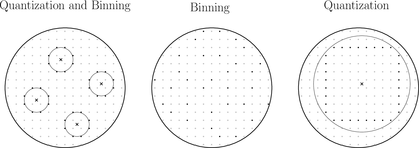
In the previous section, we have linked the DHT reliability function to that of CD. In this section, we derive bounds on the latter using random coding arguments, to wit, choosing of size at random, and analyzing the average error probabilities. To obtain good bounds for the DHT problem, however, the random ensemble should be chosen with some attention. We now list the encoding schemes typically analyzed for DHT systems, and state the corresponding CD ensemble for each of them, allowing a DHT system to be constructed (for vectors of the given input type) via its permutations:
- 1.
Binning - meaning assigning source vectors to bins uniformly at random. This corresponds to an ordinary ensemble, i.e., choosing the codewords uniformly at random over .
- 2.
Quantization - meaning assigning “close” source vectors to the same bin. This corresponds to a conditional ensemble, i.e., choosing the codewords uniformly at random in some given a “cloud center” .
- 3.
Quantization-and-binning which combines both. This corresponds to an hierarchical ensemble - a combination of the ordinary and conditional ensembles - i.e., choosing cloud centers from the ordinary ensemble over uniformly at random, and then draw “satellite” codewords for each center from the conditional ensemble uniformly at random (independently over clouds).
See Fig. 3 for illustration.
In what follows, we will analyze the hierarchical ensemble since, as discussed in the introduction, the best known achievable bounds for DHT systems are obtained via quantization-and-binning-based schemes. Furthermore, it generalizes both the ordinary ensemble and the conditional ensemble. We next rigorously define the specific hierarchical ensemble used:
Definition 7.
A fixed-composition hierarchical ensemble for an input type and rate is defined by a conditional type , where is an auxiliary random variable , a cloud-center rate and a satellite rate , such that . A random codebook from this ensemble is drawn in two stages. First, cloud centers are drawn, independently and uniformly over . Second, for each of the cloud centers , satellites are drawn independently and uniformly over .
Evidently, codewords which pertain to the same cloud are dependent, whereas codewords from different clouds are independent. Further, the ordinary ensemble is obtained as a special case by choosing and , and the conditional ensemble is obtained by setting . Whenever the CD code is to be used as bins of a DHT system for source vectors of type the correspondence between the parameters is as follows: A quantization-and-binning DHT system of rate , binning rate , and quantization rate , requires hierarchical CD codes of rate , cloud-center rate and satellite rate . The cloud centers are the reproduction vectors of the DHT system, where the joint distribution of any source vector and its reproduction vector is exactly , and the choice of the test channel is used to control the distortion of the quantization.99 9 Usually in rate-distortion theory, the test channel is used to control the average distortion for some distortion measure . Here, is always chosen from and therefore the distortion between and is constant depending on .
In this section, it will be more convenient to use the parameter instead of . Using this convention, we will use, e.g., instead of for the Chernoff parameter.
To state a random-coding bound on the reliability of CD codes, we denote
| (53) |
and
| (54) |
as well as
| (55) |
For brevity, when can be understood from context, the dependency on will be omitted. Our random-coding bound is as follows.
Theorem 8.
The infimum CD reliability function is bounded as
| (56) |
The proof of Theorem 8 appears in Appendix C. We make the following comments:
- 1.
Loosely speaking, in (55), the exponent corresponds to the contribution to the error probability from codewords which belong to different cloud centers, whereas the exponent corresponds to the contribution to the error probability from codewords which belong to the same cloud center as the transmitted codeword. Thus, for a given rate , is monotonically nonincreasing with , while is monotonically non-decreasing with (or, monotonically nonincreasing with ). The cloud-center rate and the test channel therefore should be chosen to optimally balance between these two contributions to the error probability.
- 2.
In comparison to [64], we have generalized the random coding analysis of the detection error exponents to hierarchical ensembles, and also obtained simpler expressions using the ensemble average of the exponent of the Chernoff parameter.
- 3.
In fact, a stronger claim than the one appears in Theorem 8 can be made. It can be shown that there exists a single sequence of CD codes such that
(57) simultaneously for all . Thus, when using such a CD code, the operating point along the trade-off curve between the two exponents can be determined solely by the detector, and can be arbitrarily changed from block to block. For details regarding the proof of this claim, see Remark 18.
Next, we state our expurgated exponent, and to this end we denote
| (58) |
Theorem 9.
The infimum CD reliability function is bounded as
| (59) |
The proof appears in Appendix C. We make the following comments:
- 1.
A similar expurgated bound can be derived for hierarchical ensembles. However, when optimizing the rates for this expurgated bound, it turns out that choosing is optimal. Thus, the resulting bound exactly equals the bound of Theorem 9, which corresponds to an ordinary ensemble.
- 2.
Since the expurgated exponent only improves the random-coding exponent of the ordinary ensemble (which is inferior in performance to the hierarchical ensemble), it is anticipated that expurgation does not play a significant role in this problem, compared to the channel coding problem. This might be due to the fact that the aim of expurgation is to remove codewords which have “close” neighbors, while this is not actually required in the DHT problem. This can also be attributed to the bounding technique of the expurgated bound, which is based on pairwise Chernoff parameters.
After deriving the bounds on the reliability of CD, we return to the DHT problem, and conclude the section with a short proof of Theorem 2.
Proof:
Up to the arbitrariness of , Theorem 6 states that
| (60) |
Further, the random-coding bound of Theorem 8 and the expurgated bound of Theorem 9 both imply that
| (61) | ||||
| (62) |
The bound of Theorem 2 is obtained by substituting in (62) in (60), while changing variables from to and from to , as well as using the definitions of (27), (30) and (31). ∎
VI Computational Aspects and a Numerical Example
The bound of Theorem 2 is rather involved, and therefore it is of interest to discuss how to compute it efficiently. Evidently, the main computational task is the computation of and for a given . To this end, it can be seen that the objective functions of both and are convex functions of (and strictly convex, if ).1010 10 Indeed, the divergence terms and are convex in . The term is also convex in , as a composition of a linear function which maps to and the mutual information . The pointwise maximum of two convex functions is also a convex function (note that ). Furthermore, the feasible set of is a convex set (only has linear constraints) and thus the computation of is a convex optimization problem, which can be solved efficiently [12]. However, the feasible set of is not convex, due to the additional constraint beyond the linear constraints. Nevertheless, the value of can be computed efficiently, by only solving convex optimization problems, according to the following algorithm:
- 1.
Solve the optimization problem (28) defining , and let the optimal value be .
- 2.
Solve the optimization problem (29) defining , but without the constraint (this is a convex optimization problem). Let the solution be and the optimal value be . If then set , and otherwise, set .
- 3.
The result is .
The correctness of the algorithm follows from the following argument. It is easily verified that if then the constraint is inactive, and therefore can be omitted. Thus, in this case . However, if this is not the case, then the solution must be on the boundary, i.e., must satisfy . This is because the objective in is a convex function. In the latter case, it can be easily seen that , and as is the minimum between the two, can be set.
Given the value of , the next step is to optimize over and . While this should be done exhaustively,1111 11 Or by any other general-purpose global optimization algorithm. any specific choice of and (or a restricted optimization set for them) leads to an achievable bound on . It should be mentioned, however, that it is not clear to us how to apply standard cardinality-bounding techniques (i.e., those based on the support lemma [18, p. 310]) to bound in this problem. Thus, in principle, the cardinality of is unrestricted, improved bounds are possible. Computing of (30) is a convex optimization problem, over .
Finally, both and should be optimized, which is feasible when is not very large and exhausting the simplex in search of the minimizer is possible. Furthermore, as we have seen in Corollary 4, when only Stein’s exponent is of interest, i.e., , the minimal value in (32) must be attained for . Thus, there is no need to minimize over , but rather only on . We can also set if the weak version (39) of Corollary 4 is used as a bound. More generally, the minimizer of must satisfy , and this can decrease the size of the feasible set of whenever the required is not very large.
A simple example for using the above methods to compute bounds on the DHT reliability function is given as follows.
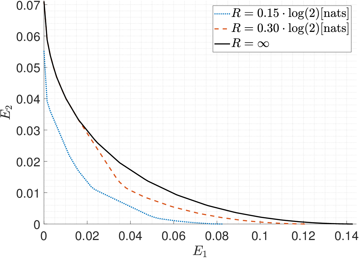
Example 10.
Consider the case , and , where and are binary symmetric channels with crossover probabilities and , respectively. We have used an auxiliary alphabet of size , and due to the symmetry in the problem, we have only optimized over symmetric . The random-coding bounds on the reliability of the DHT is shown in Fig. 4 for two different rates. The convex optimization problems were solved using CVX, a Matlab package for disciplined convex programming [21].
VII Conclusion and Further Research
We have considered the trade-off between the two types of error exponents of a DHT system, with full side information. We have shown that its reliability is intimately related to the reliability of CD, and thus the latter simpler problem should be considered. Achievable bounds on the reliability of CD were derived, under the optimal Neyman-Pearson detector.
There are multiple directions in which our understanding of the problem can be broadened:
- 1.
Variable-rate coding: The DLC reliability may be increased when variable rate is allowed, either with an average rate constraint [13], or under excess-rate exponent constraint [63]. It is interesting to use the techniques developed for the DLC to the DHT problem (see also the discussion in [65, Appendix]).
- 2.
Computation of the bounds: The main challenge in the random-coding bound computation is the optimization over the test channel . First, deriving cardinality bounds on the auxiliary random variable alphabet is of interest. Second, finding an efficient algorithm to optimize the test channel, perhaps an alternating-maximization algorithm in the spirit of the Csiszár-Tusnády [20] and the Blahut-Arimoto algorithms [6, 7, 10]. As was noted in [56, 33], Stein’s exponent in the DHT problem of testing against independence is identical to the information bottleneck problem [57], for which such alternating-maximization algorithm was developed.
- 3.
Converse bounds: We have shown converse bounds on the reliability of DHT systems, it suffices to obtain converse bounds on the reliability of CD codes, no concrete bounds were derived. To obtain converse bounds which explicitly depend on the rate (in contrast to Proposition 1), two challenges are visible. First, it is tempting to conjecture that the Chernoff characterization (10) characterizes the reliability of CD codes, in the sense that1212 12 As usual is the subsequence of blocklength such that is not empty.
(63) just as a similar quantity was used to derive the random-coding and expurgated bounds. Second, even if this conjecture holds, the value of
(64) should be lower bounded for all CD codes whose size is larger than . As this term can be identified as a Rényi divergence [44, 59], the problem of bounding its value is a Rényi divergence characterization. This problem seems formidable, as the methods developed in [4] for the entropy characterization problem rely heavily on the chain rule of mutual information; a property which is not naturally satisfied by Rényi entropies and divergences. Hence, the problem of obtaining a non trivial converse bound for the reliability of DHT systems with general hypotheses and a positive encoding rate remains an elusive open problem.
- 4.
Rate constraint on the side information: The reliability of a DHT systems in which the side-information vector is also encoded at a limited rate should be studied under optimal detection. Such systems will naturally lead to multiple-access CD codes, as studied for ordinary channel coding (see [39, 40] and references therein). However, for such a scenario, it was shown in [25] that the use of linear codes (a-la Körner-Marton coding) dramatically improves performance. Thus, it is of interest to analyze DHT systems with both linear codes and optimal detection. However, it is not yet known how to apply the type-enumeration method, used here for analysis of optimal detection, to linear codes. Hence, either the type-enumeration method should be refined, or an alternative approach should be sought after.
- 5.
Generalized hypotheses: Hypotheses regarding the distributions of continuous random variables, or regarding the distributions of sources with memory can be considered. Furthermore, the case of composite hypotheses, in which the distribution under each hypotheses is not exactly known (e.g., belongs to a subset of a given parametric family), and finding universal detectors which operate as well as the for simple hypotheses can also be considered. For preliminary results along this line see [48, 64].
Acknowledgment
Discussions with N. Merhav, the comments of the associate editor, A. Tchamkerten, and the comments of the anonymous reviewers, are acknowledged with thanks.
Appendix A Proofs of Corollaries to Theorem 2
Proof:
Suppose that the inner minimization in the bound of Theorem 2 is dominated by for all . Then, (32) reads
| (A.1) | ||||
| (A.2) | ||||
| (A.3) | ||||
| (A.4) | ||||
| (A.5) |
where: follows since (see (C.31) in the proof of Lemma 16)
| (A.6) | ||||
| (A.7) |
follows since the objective function is linear in (and hence concave) and convex in , and therefore the minimization and maximization order can be interchanged [51]. Thus, the achievability bound of Theorem 2 coincides with the converse bound of Proposition 1, where the latter is obtained when the rate of the DHT system is not constrained at all, and given by the reliability function of the ordinary HT problem between and . ∎
Proof:
It can be seen that the outermost minimum in (32) must be attained for . Intuitively, since we are only interested in negligible type 1 exponent, any event with has exponentially decaying probability , and does not affect the exponent. More rigorously, if then by taking the objective function becomes unbounded. Hence (38) immediately follows. Further simplifications are possible if the bound is weakened by ignoring the expurgated term, i.e., setting in (31). In this case, since
| (A.8) |
[see (A.7)], and since only multiplies positive terms in the objective functions of [see (28) and (29)], it is evident that the supremum in (38) is obtained as . Hence, the supremum and minimum in (38) can be interchanged to yield the bound
| (A.9) | ||||
| (A.10) |
where follows since
| (A.11) | ||||
| (A.12) | ||||
| (A.13) |
∎
Appendix B Proof of Theorem 6
B-A Proof of the Achievability Part
In the course of the proof , we will use subcodes of CD codes, and would like to claim that the error probabilities of these subcodes is not significantly different than the code itself. The following lemma establish such a property.
Lemma 11.
Let be a CD code, and be a detector. Then, there exists a CD code with which satisfies the following: For any subcode , there exists a of detector such that
| (B.1) |
holds for both .
Proof:
Note that the error probabilities in (44) and (45) are averaged over the transmitted codeword . We first prove that by expurgating enough codewords from a codebook with good average error probabilities, a codebook with maximal (over the codewords) error probabilities can be obtained (for both types of error). The proof follows the standard expurgation argument from average error probability to maximal error probability (which in turn follows from Markov’s inequality). Denoting the conditional type 1 error probability by1313 13 Note that conditioned on , depends on the code only if the detector depends on the code. In this lemma, the detector is arbitrary, and the use of this notation is therefore just for the sake of consistency.
| (B.2) |
we may write
| (B.3) | ||||
| (B.4) |
Thus, at least of the codewords in satisfy
| (B.5) |
Using a similar notation for the conditional type 2 error probability, and repeating the same argument, we deduce that there exists such that and both (B.5) as well as
| (B.6) |
hold for any . Let us now consider any . For the code , the detector is possibly suboptimal, and thus might be improved. Using the standard Neyman-Pearson lemma [42, Prop. II.D.1], one can find a detector (perhaps randomized) to match any prescribed type 1 error probability value, which is optimal in the sense that if any other detector satisfies then . Specifically, let us require that
| (B.7) |
and choose . Then, as (B.5) holds for any ,
| (B.8) | ||||
| (B.9) | ||||
| (B.10) |
and as is optimal in the Neyman-Pearson sense, (B.6) implies that
| (B.11) | ||||
| (B.12) | ||||
| (B.13) |
The result follows from (B.7) and (B.13). Note that is a valid choice. ∎Next, we focus on encoding a single type class of the source, say . Given an optimal sequence of CD codes for the input type , we construct a DHT system which has the same conditional error probabilities (given that ) by permutations of the CD code, as described in Section IV.
Lemma 12.
Let and be given, such that , and let the subsequence of blocklengths such that is not empty. Further, let be a sequence of CD codes of type and rate , and be a sequence of detectors. Then, there exist a sequence of DHT systems of rate such that
| (B.14) |
holds for both .
Proof:
We only need to focus on . For notational simplicity, let us assume that is always such that is not empty. Let us first extract from the sequence of CD codes whose existence is assured by Lemma 11. The rate of is chosen to be larger than (for all sufficiently large ), and for any given codeword, the error probability of each type is assured to be up to a factor of of its average error probability.
Recall the definition of permutation of in (51) and (52). As , clearly so is for any , and thus, there exists a set of permutations such that
| (B.15) |
By a simple counting argument, the minimal number of permutations required is at least . This is achieved when the permuted sets are pairwise disjoint, i.e., , for all . While this property is difficult to assure, Ahlswede’s covering lemma [1, Section 6, Covering Lemma 2] (see also [2, Sec. 3, Covering Lemma]) implies that up to the first order in the exponent, this minimal number can be achieved. In particular, there exists a set of permutations such that
| (B.16) |
for all sufficiently large. Without loss of generality (w.l.o.g.), we assume that is the identity permutation, and thus . Further, for , we let
| (B.17) |
In words, the code is the permutation of the code , excluding codewords which belong to a permutation of with a smaller index. Thus, forms a disjoint partition of . Moreover, Lemma 11 implies that for any given
| (B.18) |
(where is the inverse permutation of ), one can find a detector such that
| (B.19) |
and
| (B.20) |
Now, let
| (B.21) |
Since the hypotheses are memoryless, the permutation does not change the probability distributions. Indeed, for an arbitrary CD code , a detector and a permutation ,
| (B.22) | ||||
| (B.23) | ||||
| (B.24) | ||||
| (B.25) | ||||
| (B.26) | ||||
| (B.27) |
where Hence,
| (B.28) |
and
| (B.29) |
We thus construct as follows. The codes will serve as the bins of , and detectors as the decision function, given that the bin index is . As said above, only will be encoded. More rigorously, the encoding of is given by whenever , and by whenever . Clearly, the rate of the code is less than
| (B.30) |
for all sufficiently large. The detector is given by . The conditional type 1 error probability of this DHT system is given by
| (B.31) | ||||
| (B.32) | ||||
| (B.33) | ||||
| (B.34) | ||||
| (B.35) |
where follows because given the source vector is distributed uniformly over , follows from (B.28), and follows from (B.19). Similarly, the conditional type 2 error probability is upper bounded as
| (B.36) |
The factor in the error probabilities is negligible asymptotically. ∎The DHT system constructed in Lemma 12 achieves asymptotically optimal error probabilities, only conditional on , for a single . To construct a DHT system which achieves unconditional asymptotically optimal error probabilities, one can, in principle, construct a different DHT subsystem for any . Then, the encoder will choose the appropriate system according to the type of , and then inform the detector of the actual system utilized by a short header (for which the required rate is negligible since the number of types only increases polynomially). However, as clearly as , such a method might fail since the convergence of the error probabilities to their exponential bounds, may depend on the type. For example, let be a sequence of types which satisfies and for all . A priori, it might be that the error probabilities of are far from their asymptotic values, for all . In other words, uniform convergence of the error probabilities to their asymptotic exponential bounds is required.
We solve this problem (see also [63, 65]) by defining a finite grid of types for a fixed , and construct DHT subsystems only for , where . As uniform convergence of the error probabilities of for is assured. Now, if the type of belongs to , it can be encoded using . Otherwise, is slightly modified to a different vector , where the type of the latter does belong to . Then, is encoded using the DHT subsystem which pertain to its type. Since the DHT subsystems are designed for , rather than for , the side-information vector is also modified to a vector , using additional information sent from the encoder. To analyze the effect of this modification on the error probabilities, we will need the following partial mismatch lemma.
Lemma 13.
Let be a CD code, and a detector. Also fix which satisfies both and (for example, ) and let
| (B.37) |
and
| (B.38) |
Further, for , assume that is drawn as follows: Given , under both hypotheses, under the hypothesis , and under the hypothesis . Then,
| (B.39) |
and
| (B.40) |
Proof:
We will show that the “wrong” distribution of in the first coordinates does not change likelihoods and probabilities significantly. Indeed, for the type 1 error probability, conditioning on
| (B.41) |
Then, since,
| (B.42) | ||||
| (B.43) | ||||
| (B.44) |
we obtain
| (B.45) | ||||
| (B.46) | ||||
| (B.47) |
The statement regarding the type 2 error probability is similar. ∎We will also use the following lemma whose simple proof is omitted.
Lemma 14.
Let and assume that where . If then
| (B.48) |
We are now ready to prove the achievability part.
Proof:
We will describe the construction of the sequence of DHT systems. Then we will describe the encoder and show that satisfies the rate constraint. Finally, we will describe the detector and show that it satisfies the type 1 error exponent constraint, and prove that the achieved type 2 error exponent is good as the bound stated in the theorem.
Construction of a sequence of DHT systems:
- 1.
Choose a finite grid of types: Given (to be specified later), choose such that for any , where1414 14 If the minimizer is not unique, one of the minimizers can be arbitrarily and consistently chosen.
(B.49) - 2.
Let be given. For any , construct the optimal CD code of rate , and its optimal detector such that
(B.50) where . By definition of the CD reliability function, there exists such that for all
(B.51) - 3.
For any , construct a DHT subsystem such that
(B.52) and
(B.53) for all . The existence of such construction is assured by Lemma 12, using the CD codes .
The encoder operation and rate analysis: Upon observing of type , the encoder:
- 1.
Sends the detector a description of . As , this description requires no more than nats. If then no additional bits are sent (otherwise further bits are sent as follows).
- 2.
Finds and generates with a uniform distribution over the set
(B.54) Note that Lemma 14 assures that this set is not empty, and that if is distributed uniformly over then is distributed uniformly over (due to the permutation symmetry of type classes).
- 3.
Sends to the detector a description of the set . Since , the number possible sets is less than
(B.55) and so sending its description requires no more than nats.
- 4.
Sends the detector the value of for . Each letter can be encoded using nats, and so this requires no more than nats.
- 5.
Sends the message index to the detector. This requires nats.
The required rate is therefore no more than
| (B.56) |
By choosing sufficiently small, the required rate can be made less than for all sufficiently large.
The detector operation and error probability analysis: Upon receiving the message of the encoder and observing the detector:
- 1.
Decodes the type of . If then it decides on the hypothesis based on . Otherwise it continuous.
- 2.
Finds and generates as follows: For all , if then , and if then , where is as chosen in Lemma 13.
- 3.
Decides on the hypothesis as .
Note that the encoder alters to such that has a type which matches one of the subsystems , . Due to this modification, a similar change is made to the side-information vector. The detector generates a proper by using the information sent from the encoder (namely, and the values of on this set). However, for rather than according to the true distribution ( or ) . As we shall see, Lemma 13 assures that this mismatch has small effect on the error probabilities. Let us denote the constructed system by , and analyze the error probabilities for for all .
For the type 1 error exponent, note that
| (B.57) | ||||
| (B.58) | ||||
| (B.59) | ||||
| (B.60) | ||||
| (B.61) | ||||
| (B.62) |
where follows since if the detector can decide on the hypothesis with zero error, follows since and , follows from the definition of the system , follows from Lemma 13, follows from (B.52) and as for all , and follows from the fact that is a continuous function of in , and thus uniformly continuous.
For the type 2 error exponent, first note that, as for the type 1 error probability,
| (B.63) | ||||
| (B.64) |
Now,
| (B.65) | ||||
| (B.66) | ||||
| (B.67) | ||||
| (B.68) | ||||
| (B.69) | ||||
| (B.70) | ||||
| (B.71) |
where follows from Lemma 13 (and the way was generated), follows from (B.53) and as for all . Passage holds for some that satisfies as , and follows from the fact that is a continuous function of over the compact set , and thus uniformly continuous. Finally, by choosing sufficiently small, and then sufficiently small, the loss in exponents can be made arbitrarily small. ∎
B-B Proof of the Converse Part
The proof of the converse part is based upon identifying for any sequence of DHT systems a sequence of bin indices such that the size of is “typical” to , and such that the conditional error probability given is also “typical” to . The sequence of bins corresponds to a sequence of CD codes, and thus clearly cannot have better exponents than the ones dictated by the reliability function of CD codes. This restriction is then translated back to bound the reliability of DHT systems.
Proof:
For a given DHT system , let us denote the (random) bin index by . We will show that the converse hold even if the detector of the DHT systems is aware of the type of . Consequently, as an optimal Neyman-Pearson detector will only average the likelihoods of source vectors from the true type class, it can be assumed w.l.o.g. that each bin contains only sequences from a unique type class.
Recall that is the number of possible bins, and let be the number of bins associated with a specific type class , i.e., where
| (B.72) |
Further, conditioned on the type class (note that is a function of ),
| (B.73) | ||||
| (B.74) | ||||
| (B.75) | ||||
| (B.76) | ||||
| (B.77) |
as for all sufficiently large, , and thus clearly . Hence, for any , Markov’s inequality implies
| (B.78) | ||||
| (B.79) |
Thus, using (B.77), conditioned on
| (B.80) |
with probability larger than . Now, assume by contradiction that the statement of the theorem does not hold. This implies that there exists an increasing subsequence of blocklengths and such that
| (B.81) |
and
| (B.82) |
for all sufficiently large. For brevity of notation, we assume w.l.o.g. that these bounds hold for all sufficiently large, and thus omit the subscript . Let be given. Then, for all sufficiently large [which only depends on ],
| (B.83) |
for all such that is not empty. Indeed, for all sufficiently large, it holds that
| (B.84) | ||||
| (B.85) | ||||
| (B.86) | ||||
| (B.87) |
and (B.83) is obtained by rearranging. Writing
| (B.88) |
Markov’s inequality implies
| (B.89) | ||||
| (B.90) | ||||
| (B.91) |
The same arguments can be applied for the type 2 exponent. Thus, from the above and (B.80), with probability larger than , which is strictly positive for all sufficiently large , the bin index satisfies (B.80),
| (B.92) | ||||
| (B.93) |
as well as
| (B.94) |
Now, let be chosen to achieve up to , i.e., to be chosen such that
| (B.95) |
and let be the subsequence of blocklengths such that is not empty. From the above discussion, there a sequence of bin indices such that (B.80), (B.93) and (B.94) hold for . Consider the sequence of bins to be a sequence of CD codes, whose rate is larger than , its detectors are induced by the DHT system detector as , and such that
| (B.96) |
and
| (B.97) | ||||
| (B.98) |
where the last inequality follows from (B.95). However, this is a contradiction, since whenever (B.96) holds the definition of CD reliability function implies that
| (B.99) |
for all sufficiently large. ∎
Appendix C Proof of Theorems 8 and 9
We will prove the random-coding bound of Theorem 8 by considering CD codes drawn from the fixed-composition hierarchical ensemble defined in Definition 7. In the course of the proof, we shall consider various types of the form and . All of them are assume to have marginal even if it is not explicitly stated. Furthermore, we shall assume that the blocklength is such that is not empty. In this case, the notation for exponential equality (or inequality) needs to be clarified as follows. We will say that if
| (C.1) |
where is the subsequence of blocklengths such that is not empty.
The proof of Theorem 8 relies on the following result, which is stated and proved by means of the type-enumeration method (see [37, Sec. 6.3]). Specifically, for a given , we define type-class enumerators for a random CD code by
| (C.2) |
To wit, counts the random number of codewords whose joint type with their own cloud center and is . To derive a random-coding bound on the achievable CD exponents, we will need to evaluate the exponential order of for an arbitrary sequence of taken from .
The result is summarized in the following proposition, interesting on its own right.
Proposition 15.
Let be given for some , with and . Also let be the subsequence of blocklengths such that and are both not empty, and let satisfy for all . Then, for any
| (C.3) |
where
| (C.4) |
It is interesting to note that the expression (C.3) is not continuous, as, say, . The proof of Proposition 15 is of technical nature, and thus relegated to Appendix D. For the rest of the proof, no knowledge of the type-enumeration method is required.
As described in Section IV the detector of a CD code faces an ordinary HT problem between the and , and therefore the exponents of this HT problem are simply given by (6) and (7) (when letting ). In turn, using the characterization (10), the reliability function can be expressed using the Chernoff parameter between and . We thus next analyze the average exponent of the Chernoff parameter over a random choice of CD codes.
Lemma 16.
Proof:
Let us denote the log-likelihood of by
| (C.6) | ||||
| (C.7) |
and the log-likelihood of by (with replacing ). For any given ,
| (C.8) | ||||
| (C.9) | ||||
| (C.10) | ||||
| (C.11) | ||||
| (C.12) | ||||
| (C.13) | ||||
| (C.14) | ||||
| (C.15) | ||||
| (C.16) |
where follows since by symmetry, the expectation only depends on the type of , and by using the definitions of the enumerators in (C.2), and the log-likelihood in (C.6). After passage and onward, is an arbitrary member of , and the sums and maximization operators are over restricted to the set
| (C.17) |
In the last equality we have implicitly defined and . By defining
| (C.18) |
and using standard arguments (e.g., as in the proof of Sanov’s theorem [14, Theorem 11.4.1]) we get
| (C.19) |
The result (C.5) will follow by minimizing
| (C.20) | ||||
| (C.21) |
over . We now evaluate this expression in three cases, which correspond to the three cases of Proposition 15. In each one, we substitute for the appropriate term,1515 15 In fact, Proposition 15 implies that the limit inferior of this sequence is a proper limit. as follows:
- Case 1.
For ,
(C.22) (C.23) (C.24) where follows from the identity
(C.25) By defining the distribution
(C.26) and observing that
(C.27) (C.28) it is evident that
(C.29) (C.30) (C.31) - Case 2.
- Case 3.
For and
(C.36) (C.37)
Hence, the required bound on the Chernoff parameter is given by
| (C.38) |
Observing (C.37), we note that the third term in (C.38) satisfies
| (C.39) | ||||
| (C.40) |
where in we have removed the constraint in the first term of the outer minimization, since for with the second term will dominate the minimization. Thus, the first term in (C.40) may be unified with the second term of (C.38). Doing so, the constraint may be removed in the second term of (C.38). Consequently, the required bound on the Chernoff parameter is given by
| (C.41) |
The second term in (C.41) corresponds to defined in (53). The third term corresponds to defined in (54), when using , and noting that when , it is equal to
| (C.42) |
Using the definition (55) of as the minimum of the last two cases, (C.5) is obtained. ∎Next, recall that by its definition, a valid CD code of rate is comprised of distinct codewords. However, when the codewords are independently drawn, some of them might be identical. Nonetheless, the next lemma shows that the average number of distinct codewords of a randomly chosen code is asymptotically close to .
Lemma 17.
Let be drawn randomly from the hierarchical ensemble of Definition 7, with conditional distribution , cloud-center rate , and satellite rate (which satisfy ). If then
| (C.43) |
Proof:
Let us enumerate the random cloud centers as and the random satellite codebooks as . For any given
| (C.44) | ||||
| (C.45) | ||||
| (C.46) |
using [53, Lemma 1]. Further, for a random cloud center and
| (C.47) | ||||
| (C.48) | ||||
| (C.49) | ||||
| (C.50) | ||||
| (C.51) |
where is due to symmetry, and the definition
| (C.52) | ||||
| (C.53) |
Therefore, the average number of distinct codewords in the random CD code is lower bounded as
| (C.54) | ||||
| (C.55) | ||||
| (C.56) | ||||
| (C.57) | ||||
| (C.58) | ||||
| (C.59) | ||||
| (C.60) |
where holds since for a given set of pairwise independent events [50, Lemma A.2]
| (C.61) |
The passage follows from the assumptions and . Thus, on the average, a randomly chosen has more than distinct codewords. The results follows since clearly . ∎We are now ready to prove Theorem 8. The main argument is to show that by randomly drawing a set of codewords from the hierarchical ensemble, and then removing its duplicates, i.e., keeping only a single instance of codewords which were drawn more than once (thus making it a valid CD code), may only cause a negligible loss in the achieved exponent.
Proof:
Let be given, let be the achiever of the maximum on the right-hand side of (56), and let and be the achievers of the supremum, up to . As noted in Section IV, given a CD code , the detector faces an ordinary HT problem between the distributions and , and thus the bounds of Section II-B can be used. Specifically, (10) (with ) implies that
| (C.62) | ||||
| (C.63) |
Instead of maximizing over , we use ensemble averages. To this end, let us consider a sequence of conditional type-classes such that as (as the types are dense in the simplex, such a sequence always exists). Furthermore, there exists a sequence with such that where . Then, using Lemma 16 for the hierarchical ensemble defined by rates and types we obtain that
| (C.64) |
and using Lemma 17, we obtain that the average number of distinct codewords in a randomly chosen codebook is . It remains to prove the existence of a CD code, whose codewords are all distinct, and its Chernoff parameter exponent is close to the ensemble average. To this end, consider the events
| (C.65) |
and
| (C.66) |
where, for brevity, we denote . Note that since , for all sufficiently large, the reverse Markov inequality1616 16 The reverse Markov inequality states that if for some . Then, for any , [35, Section 9.3, p. 159] implies that
| (C.67) |
Further, Markov’s inequality implies that for all sufficiently large
| (C.68) |
Then, we note that
| (C.69) | ||||
| (C.70) | ||||
| (C.71) | ||||
| (C.72) |
and thus deduce that there exists a CD code such that and holds for all sufficiently large. Let the CD code obtained after keeping only the unique codewords of be denoted as . It remains to show that the exponent of the Chernoff parameter of is asymptotically equal to that of . Indeed,
| (C.73) | ||||
| (C.74) | ||||
| (C.75) |
where follows since , and follows since , and therefore
| (C.76) |
With the above, the derivation of (C.63) may be continued as
| (C.77) | ||||
| (C.78) |
Now, taking the limit over ’s such that is not empty,
| (C.79) | ||||
| (C.80) | ||||
| (C.81) |
where the first equality follows from the continuity of in (which can be readily verified from (53) and (54)), and the second inequality from the definition of . The proof is completed by taking . ∎
Remark 18.
As mentioned after Theorem 8, the random-coding bound can be achieved by a single sequence of CD codes, simultaneously for all type 1 error exponent constraint . This can be proved by showing that there exists a CD code such that the event defined in (C.68) holds for all . To show the latter, we uniformly quantize the interval to with and a fixed . Then, using the union bound, for all sufficiently large
| (C.82) | ||||
| (C.83) | ||||
| (C.84) |
and this bound can be used in lieu of (C.68) in the proof. This will prove the simultaneous achievability of for all . Then, utilizing the continuity of , by taking to increase sub-exponentially in the same result can be established to the entire interval.
Appendix D The Type-Enumeration Method and the Proof of Proposition 15
We begin with a short review of the type-enumeration method [37, Sec. 6.3]. To begin, let us define type-class enumerators for the cloud centers by
| (D.1) |
To wit, counts the random number of cloud centers which have joint type with . While defined in (C.2) is an enumerator of a hierarchical ensemble, is an enumerator of an ordinary ensemble, and thus simpler to analyze. Furthermore, the analysis of depends on the properties of , and thus we begin by analyzing the latter.
As the cloud centers in the ensemble are drawn independently, is a binomial random variable. It pertains to trials and probability of success of the exponential order of , and consequently, . In the sequel, we will need refined properties of the enumerator, and specifically, its large-deviations behavior and the moments . To this end, we note that as is just an enumerator for a code drawn from an ordinary ensemble, the analysis of [37, Sec. 6.3] [36, Appendix A.2] holds. As was shown there, when , increases exponentially with as , and concentrates double-exponentially rapidly around this average. Specifically, letting
| (D.2) |
then for any sufficiently small
| (D.3) |
When holds, decreases exponentially with as , and almost surely. Furthermore, the probability that even a single codeword has joint type with is exponentially small, and the probability that there is an exponential number of such codewords is double-exponentially small. Specifically, for all sufficiently large
| (D.4) |
and for any given
| (D.5) |
Using the properties above, it can be easily deduced that
| (D.6) |
or, in an equivalent and more compact form,
| (D.7) |
We can now turn to analyze the behavior of the more complicated enumerator . To this end, note that conditioned on the event is a binomial random variable pertaining to trials and probability of success of the exponential order of . Thus,
| (D.8) |
and the conditional large-deviations behavior of is identical to the large-deviations behavior of , with and replacing and , respectively. The next lemma provides an asymptotic expression for the unconditional moments of . It can be easily seen that (D.7) is obtained as a special case, when setting and .
Lemma 19.
For
| (D.9) |
Proof:
Let
| (D.10) |
define the events
| (D.11) |
| (D.12) |
| (D.13) |
and recall the definition of the event in (D.2). We will consider four cases depending on the relations between the rates and mutual information values. For the sake of brevity, only the first case will be analyzed with a strictly positive and then the limit will be taken. In all other three cases, we shall derive the expressions for the moments assuming , with the understanding that upper and lower bounds can be derived in a similar manner to the first case. For notational convenience, when the expressions are derived assuming we will omit from the notation of the events defined above [e.g., ]. We will use the moments (D.6), the strong concentration relation (D.3) and the large-deviations bound (D.4), for both and [when the latter is conditioned on the value of ].
- Case 1.
If and , then for all sufficiently small, and and thus,
(D.14) (D.15) (D.16) Similarly, it can be shown that
(D.17) As is arbitrary, we obtain
(D.18) - Case 2.
If and then
(D.19) (D.20) (D.21) (D.22) (D.23) - Case 3.
If and then
(D.24) (D.25) (D.26) - Case 4.
If and then
(D.27) (D.28) (D.29) (D.30)
Noting that is equivalent to , it is easy to verify that
| (D.31) |
matches all four cases. The final expression is obtained from the identities
| (D.32) | ||||
| (D.33) | ||||
| (D.34) |
where follows from the identity with , follows from the same identity with , and follows from with and . ∎To continue, we will need to separate the analysis according to whether (Lemma 22) or (Lemma 25). In the former case and count codewords which pertain to different cloud centers, and as we shall next see, and are asymptotically uncorrelated. In the later case, these enumerators may count codewords which pertain to the same cloud center, and correlation between and is possible. We will need two auxiliary lemmas.
Lemma 20.
Let be a monotonically non-decreasing function, let and with . Then,
| (D.35) |
Proof:
Let and , independent of . As the sum of independent binomial random variables with the same success probability is also binomially distributed, we have is equal in distribution to . Thus,
| (D.36) | ||||
| (D.37) |
where the inequality holds pointwise for any given , and thus also under expectation. ∎As is well known from the method of types, . The next lemma shows that this probability can be upper bounded asymptotically even when , and the large-deviations behavior does not hold.
Lemma 21.
Let be given such that and . Also let and assume that is distributed uniformly over . Then, for any given there exists such that for all
| (D.38) |
Proof:
Using Robbins’ sharpening of Stirling’s formula (e.g., [18, Problem 2.2]), it can be shown that the size of a type class satisfies
| (D.39) |
Hence,
| (D.40) | ||||
| (D.41) | ||||
| (D.42) |
where holds by symmetry [assuming that is drawn uniformly over ].
Now, by the Kullback-Csiszár-Kemperman-Pinsker inequality [14, Lemma 11.6.1][18, Exercise 3.18]
| (D.43) | ||||
| (D.44) |
and thus for any given
| (D.45) | ||||
| (D.46) |
where . Choose such that for all . We consider two cases:
- Case 1.
If then it is elementary to verify that in this event, as and was assumed,
(D.47) (D.48) and thus (D.42) implies that
(D.49) - Case 2.
If then and
(D.50)
This completes the proof. ∎We are now ready to state and prove the asymptotic uncorrelation lemma for .
Lemma 22.
Let be given such that . Then,
| (D.51) |
Proof:
We begin by lower bounding the correlation. To this end, let us decompose
| (D.52) |
where is the enumerator of to the subcode of of codewords which pertain to half of the cloud centers (say, for cloud centers with odd indices) and is the enumerator pertaining to the rest of the codewords. Note that and are independent for any given . Hence,
| (D.53) | ||||
| (D.54) | ||||
| (D.55) | ||||
| (D.56) |
where follows since enumerators are positive, and follows since and are independent for any given . holds true since () pertain to codebooks of cloud-center size and satellite rate , and thus clearly
To derive an upper bound on the correlation, we first note two properties. First, as the codewords enumerated by necessarily correspond to different cloud centers from the codewords enumerated by , the following Markov relation holds:
| (D.57) |
Second, conditioned on , is a binomial random variable pertaining to trials with a probability of success given by
| (D.58) |
However, this probability is not significantly different than the unconditional probability. More rigorously, for any and all sufficiently large
| (D.59) |
To see this, note that since we must have , and thus Lemma 21 implies that for any and all sufficiently large
| (D.60) | ||||
| (D.61) | ||||
| (D.62) |
and, similarly,
| (D.63) |
Equipped with the Markov relation (D.57) and the bound on the conditional probability (D.59), we can derive an upper bound on the correlation that asymptotically matches the lower bound (D.56), and thus prove the lemma. Indeed,
| (D.64) | ||||
| (D.65) | ||||
| (D.66) | ||||
| (D.67) | ||||
| (D.68) | ||||
| (D.69) |
where and follows from the law of total expectation, and follows from the Markov relation (D.57). To see note that is a non-decreasing function of [see (D.8)]. In addition, conditioned on , is a binomial random variable pertaining to less trials. Thus, follows from Lemma 20. We now note that
| (D.70) |
and
| (D.71) |
are both moments of binomial random variables with the same number of trials, but the former has a success probability
| (D.72) |
and the latter has a success probability
| (D.73) |
However, (D.59) shows that the latter success probability has the same exponential order. In turn, the proof of Lemma 19 shows that the exponential order of this expectation only depends on the exponential order of the success probability. Consequently,
| (D.74) | ||||
| (D.75) |
Using this in (D.69) completes the proof. ∎Next, we move to the case where the cloud centers may be the same, i.e., . In this case, correlation between and is possible even asymptotically. Apparently, this is due to the fact that with high probability whenever , and thus, in this case, with high probability. However, as we will next show, and are asymptotically uncorrelated when conditioned on .
To show this, we first need a result analogous to Lemma 21. To this end, we first need to exclude possible from the discussion. Let us say that is a joint-distribution-dictator (JDD) pair if it determines unambiguously. For example, when , corresponds to a Z-channel and corresponds to an S-channel,1717 17 That is and all other transition probabilities are non-zero. is a JDD pair. Clearly, in this case no exists with the same and marginals, and thus such are of no interest to the current discussion.
By carefully observing the Z-channel/S-channel example above, it is easy to verify if for all either or then is a JDD pair. Therefore, if is not a JDD pair then there must exist such that both and . This property will be used in the proof of the following lemma.
Lemma 23.
Let be given such that , , and is not a JDD pair. Also, let and assume that is distributed uniformly over . Then, for any given there exists such that for all
| (D.76) |
Proof:
Had been distributed uniformly over , the claim would follow directly from Lemma 21, where and there are replaced by and , respectively. However, since is distributed uniformly over the proof is not immediate. Nonetheless, it follows the same lines, and thus we will only highlight the required modifications.
Just as in (D.39), the size of a conditional type class can be shown to satisfy
| (D.77) |
and thus
| (D.78) | ||||
| (D.79) | ||||
| (D.80) |
where
| (D.81) |
Now, suppose that . Then,
| (D.82) | ||||
| (D.83) | ||||
| (D.84) | ||||
| (D.85) |
where follows since for all , and follows since is not a JDD pair, and thus there must exist such that both and (as noted before the statement of the lemma). Thus, when we get
| (D.86) |
The proof then may continue as the proof of Lemma 21. One can find sufficiently small such that any has the same support as (at least conditioned on ). Further, one can find such that
| (D.87) |
and the two cases considered in Lemma 21 can be considered here as well. In the first case, may vanish, but and thus (D.86) holds. In the second case , and thus for any given there exists such that
| (D.88) |
for all . ∎
Lemma 24.
Let be given such that . Then,
| (D.89) |
Proof:
The proof follows the same lines of the proof of Lemma 22, and so we only provide a brief outline. For a lower bound on the conditional correlation, one can decompose
| (D.90) |
where [respectively, ] corresponds to codewords of odd (even) satellite indices (say).
For a asymptotically matching upper bound on the correlation, we note that similarly to (D.59), when is drawn uniformly over ,
| (D.91) |
is close to the unconditional probability, in the sense that for any given ,
| (D.92) |
To prove this, a derivation similar to (D.62) can be used, while noting that is not a JDD pair, and so according to Lemma 23
| (D.93) |
for all sufficiently large. Equipped with these results, we get
| (D.94) | ||||
| (D.95) | ||||
| (D.96) |
where follows from the law of total expectation. For note that conditioned on both , is a binomial random variable pertaining to trials. Thus, is a non-increasing function of [see (D.8)], and follows from Lemma 20. For , we note that from (D.92), the conditioning on does not change the exponential order of the success probability of . As evident from (D.8), this conditioning can be removed without changing the exponential order of the expression. ∎Proceeding with the case of , we next evaluate the expectation over . We show that the asymptotic uncorrelation result of Lemma 22 holds, albeit with a correction term required when .
Lemma 25.
Let , and be given such that . Then,
| (D.97) |
Proof:
We consider two cases separately. First suppose that . In this case, concentrates double-exponentially fast around its expected value, where the latter equals up to the first order in the exponent. Thus, the conditional expectation and the unconditional expectation are equal up to the first order in the exponent. More rigorously, let be given and recall the definition of the event in (D.2). Then,
| (D.98) | ||||
| (D.99) | ||||
| (D.100) |
where follows from the fact decays double-exponentially [see (D.3)], and follows from (D.8). Similarly
| (D.101) |
Thus,
| (D.102) | ||||
| (D.103) | ||||
| (D.104) | ||||
| (D.105) | ||||
| (D.106) | ||||
| (D.107) | ||||
| (D.108) |
where and follow from (D.3), follows from Lemma 24, from (D.8), and from (D.100) and (D.101).
We next address the case . In this case, with high probability, with probability , and with probability double-exponentially small [see (D.4) and (D.5)]. For brevity, we will use the definitions of , and in (D.11)-(D.13). Then,
| (D.109) | ||||
| (D.110) | ||||
| (D.111) |
where for and we apply (D.5) and (D.8), respectively. Similarly,
| (D.112) |
Then,
| (D.113) | ||||
| (D.114) | ||||
| (D.115) |
where follows from a derivation similar to (D.108), and follows from (D.4).
Analogous asymptotic lower bounds on for both cases can be obtained in the same manner, when is replaced by . The proof is then completed by taking . ∎Using all the above, we are now ready to prove Proposition 15.
Proof:
For the first case of (C.3)
| (D.116) |
and the result follows from Lemma 19 with . For the second case, using Lemma 22
| (D.117) |
and the result follows from Lemma 19. Similarly, the third case follows from Lemmas 25 and 19. Specifically, the result is just as in the second case, except for the correction term to the exponent. Standard manipulations lead to the expression shown in the third case. ∎
References
- [1] R. Ahlswede. Coloring hypergraphs: A new approach to multi-user source coding, part II. Journal of Combinatorics, 5:220–268, 1980.
- [2] R. Ahlswede and I. Csiszár. Hypothesis testing with communication constraints. IEEE Transactions on Information Theory, 32(4):533–542, July 1986.
- [3] R. Ahlswede and G. Dueck. Good codes can be produced by a few permutations. IEEE Transactions on Information Theory, 28(3):430–443, May 1982.
- [4] R. Ahlswede, P. Gács, and J. Körner. Bounds on conditional probabilities with applications in multi-user communication. Probability Theory and Related Fields, 34(2):157–177, 1976.
- [5] R. Ahlswede and J. Körner. Source coding with side information and a converse for degraded broadcast channels. IEEE Transactions on Information Theory, 21(6):629–637, November 1975.
- [6] S. Arimoto. An algorithm for computing the capacity of arbitrary discrete memoryless channels. IEEE Transactions on Information Theory, 18(1):14–20, 1972.
- [7] S. Arimoto. Computation of random coding exponent functions. IEEE Transactions on Information Theory, 22(6):665–671, November 1976.
- [8] T. Berger. Decentralized estimation and decision theory. In IEEE Seven Springs Workshop on Information Theory, Mt. Kisco, NY, 1979.
- [9] P. Bergmans. Random coding theorem for broadcast channels with degraded components. IEEE Transactions on Information Theory, 19(2):197–207, March 1973.
- [10] R. E. Blahut. Computation of channel capacity and rate-distortion functions. IEEE Transactions on Information Theory, 18(4):460–473, 1972.
- [11] R. E. Blahut. Hypothesis testing and information theory. IEEE Transactions on Information Theory, 20(4):405–417, July 1974.
- [12] S. P. Boyd and L. Vandenberghe. Convex Optimization. Cambridge university press, Cambridge, U.K., 2004.
- [13] J. Chen, D. He, A. Jagmohan, and L. A. Lastras-Montaño. On the reliability function of variable-rate Slepian-Wolf coding. In Proc. of 45th Annual Allerton Conference Communication, Control, and Computing, September 2007.
- [14] T. M. Cover and J. A. Thomas. Elements of Information Theory (Wiley Series in Telecommunications and Signal Processing). Wiley-Interscience, New York, N.Y., U.S.A., 2006.
- [15] I. Csiszár. The method of types. IEEE Transactions on Information Theory, 44(6):2505–2523, October 1998.
- [16] I. Csiszár and J. Körner. Towards a general theory of source networks. Information Theory, IEEE Transactions on, 26(2):155–165, March 1980.
- [17] I. Csiszár and J. Körner. Graph decomposition: A new key to coding theorems. IEEE Transactions on Information Theory, 27(1):5–12, January 1981.
- [18] I. Csiszár and J. Körner. Information Theory: Coding Theorems for Discrete Memoryless Systems. Cambridge University Press, Cambridge, U.K., 2011.
- [19] I. Csiszár and P. C. Shields. Information Theory and Statistics: A Tutorial. Foundations and Trends in Communications and Information Theory. Now Publishers Inc, 2004.
- [20] I. Csiszár and G. Tusnády. Information Geometry and Alternating Minimization Procedures. Statistics and Decisions, Supplement Issue 1, 1984.
- [21] Inc. CVX Research. CVX: Matlab software for disciplined convex programming, version 2.0. http://cvxr.com/cvx, 2012.
- [22] A. El Gamal and Y. Kim. Network information theory. Cambridge university press, Cambridge, U.K., 2011.
- [23] R. G. Gallager. Source coding with side information and universal coding. LIDS- P-937, M.I.T., 1976. Available online: http://web.mit.edu/gallager/www/papers/paper5.pdf.
- [24] S. I. Gel’fand and M. S. Pinsker. Coding of sources on the basis of observations with incomplete information. Problemy Peredachi Informatsii, 15(2):45–57, 1979.
- [25] E. Haim and Y. Kochman. Binary distributed hypothesis testing via Körner-Marton coding. In Proc. IEEE Information Theory Workshop (ITW), pages 146–150, Septmber 2016.
- [26] T. S. Han. Hypothesis testing with multiterminal data compression. IEEE Transactions on Information Theory, 33(6):759–772, November 1987.
- [27] T. S. Han and S. Amari. Statistical inference under multiterminal data compression. IEEE Transactions on Information Theory, 44(6):2300–2324, October 1998.
- [28] T. S. Han and K. Kobayashi. Exponential-type error probabilities for multiterminal hypothesis testing. IEEE Transactions on Information Theory, 35(1):2–14, January 1989.
- [29] W. Hoeffding. Asymptotically optimal tests for multinomial distributions. The Annals of Mathematical Statistics, pages 369–401, 1965.
- [30] G. Katz, R. Couillet, P. Piantanida, and M. Debbah. On the necessity of binning for the distributed hypothesis testing problem. In Proc. IEEE International Symposium Information Theory (ISIT), pages 2797–2801, June 2015.
- [31] G. Katz, P. Piantanida, and M. Debbah. Collaborative distributed hypothesis testing. arXiv preprint, April 2016. Available online: http://arxiv.org/pdf/1604.01292.pdf.
- [32] G. Katz, P. Piantanida, and M. Debbah. A new approach to distributed hypothesis testing. In Proc. Asilomar Conference on Signals, Systems and Computers, pages 1365–1369, November 2016.
- [33] G. Katz, P. Piantanida, and M. Debbah. Distributed binary detection with lossy data compression. IEEE Transactions on Information Theory, 2017.
- [34] J. Körner and K. Marton. How to encode the modulo-two sum of binary sources (corresp.). IEEE Transactions on Information Theory, 25(2):219–221, March 1979.
- [35] M. Loève. Probability Theory I. Springer, New York, N.Y., U.S.A., 1977.
- [36] N. Merhav. Relations between random coding exponents and the statistical physics of random codes. IEEE Transactions on Information Theory, 55(1):83–92, January 2009.
- [37] N. Merhav. Statistical physics and information theory. Foundations and Trends in Communications and Information Theory, 6(1-2):1–212, 2009.
- [38] M. Mhanna and P. Piantanida. On secure distributed hypothesis testing. In Proc. IEEE International Symposium Information Theory (ISIT), pages 1605–1609, June 2015.
- [39] A. Nazari, A. Anastasopoulos, and S. S. Pradhan. Error exponent for multiple-access channels: Lower bounds. IEEE Transactions on Information Theory, 60(9):5095–5115, September 2014.
- [40] A. Nazari, S. S. Pradhan, and A. Anastasopoulos. Error exponent for multiple-access channels: Upper bounds. IEEE Transactions on Information Theory, 61(7):3605–3621, July 2015.
- [41] Y. Polyanskiy. Hypothesis testing via a comparator. In Proc. IEEE International Symposium Information Theory (ISIT), pages 2206–2210, July 2012. Extended version available online: http://people.lids.mit.edu/yp/homepage/data/htstruct_journal.pdf.
- [42] H. V. Poor. An Introduction to Signal Detection and Estimation. Springer-Verlag, New York, N.Y., U.S.A., 2nd edition, 1994.
- [43] M. S. Rahman and A. B. Wagner. On the optimality of binning for distributed hypothesis testing. IEEE Transactions on Information Theory, 58(10):6282–6303, October 2012.
- [44] A. Rényi. On measures of entropy and information. In Proceedings of the Fourth Berkeley Symposium on Mathematical Statistics and Probability, Volume 1: Contributions to the Theory of Statistics. The Regents of the University of California, 1961.
- [45] W. Rudin. Principles of mathematical analysis. McGraw-Hill, New York, N.Y., U.S.A., 3rd edition, 1976.
- [46] S. Salehkalaibar, M. Wigger, and R. Timo. On hypothesis testing against conditional independence with multiple decision centers. IEEE Transactions on Communications, 66(6):2409–2420, June 2018.
- [47] S. Salehkalaibar, M. Wigger, and L. Wang. Hypothesis testing in multi-hop networks. arXiv preprint, August 2017. Available online: http://arxiv.org/pdf/1708.05198.pdf.
- [48] H. M. H. Shalaby and A. Papamarcou. Multiterminal detection with zero-rate data compression. IEEE Transactions on Information Theory, 38(2):254–267, March 1992.
- [49] H. Shimokawa, T. S. Han, and S. Amari. Error bound of hypothesis testing with data compression. In Proc. IEEE International Symposium Information Theory (ISIT), pages 114–, June 1994.
- [50] N. Shulman. Communication Over an Unknown Channel via Common Broadcasting. PhD thesis, Dept. Electrical Engineering, Tel Aviv University, Tel Aviv, Israel, 2003. http://www.eng.tau.ac.il/~shulman/papers/Nadav_PhD.pdf.
- [51] M. Sion. On general minimax theorems. Pacific Journal of Mathematics, 8(1):171–176, 1958.
- [52] D. Slepian and J. K. Wolf. Noiseless coding of correlated information sources. IEEE Transactions on Information Theory, 19(4):471–480, July 1973.
- [53] A. Somekh-Baruch and N. Merhav. Achievable error exponents for the private fingerprinting game. IEEE Transactions on Information Theory, 53(5):1827–1838, May 2007.
- [54] S. Sreekumar and D. Gündüz. Distributed hypothesis testing over noisy channels. In Proc. IEEE International Symposium Information Theory (ISIT), pages 983–987, June 2017.
- [55] A. Tchamkerten, V. Chandar, and G. W. Wornell. Communication under strong asynchronism. Information Theory, IEEE Transactions on, 55(10):4508–4528, Oct 2009.
- [56] C. Tian and J. Chen. Successive refinement for hypothesis testing and lossless one-helper problem. IEEE Transactions on Information Theory, 54(10):4666–4681, October 2008.
- [57] N. Tishby, F. C. Pereira, and W. Bialek. The information bottleneck method. In Proc. of 37th Annual Allerton Conference Communication, Control, and Computing, September 1999.
- [58] E. Tuncel. On error exponents in hypothesis testing. IEEE Transactions on Information Theory, 51(8):2945–2950, August 2005.
- [59] T. Van Erven and P. Harremos. Rényi divergence and Kullback-Leibler divergence. IEEE Transactions on Information Theory, 60(7):3797–3820, 2014.
- [60] D. Wang, V. Chandar, S. Y. Chung, and G. W. Wornell. Error exponents in asynchronous communication. In Proc. 2011 IEEE International Symposium on Information Theory, pages 1071–1075, 2011.
- [61] S. Watanabe. Neyman-Pearson test for zero-rate multiterminal hypothesis testing. IEEE Transactions on Information Theory, 64(7):4923–4939, July 2018.
- [62] N. Weinberger and N. Merhav. Codeword or noise? exact random coding exponents for joint detection and decoding. IEEE Transactions on Information Theory, 60(9):5077–5094, September 2014.
- [63] N. Weinberger and N. Merhav. Optimum trade-offs between the error exponent and the excess-rate exponent of variable-rate Slepian-Wolf coding. IEEE Transactions on Information Theory, 61(4):2165–2190, April 2015. Extended version available online: http://arxiv.org/pdf/1401.0892v3.pdf.
- [64] N. Weinberger and N. Merhav. Channel detection in coded communication. IEEE Transactions on Information Theory, 63(10):6364–6392, October 2017.
- [65] N. Weinberger and N. Merhav. A large deviations approach to secure lossy compression. IEEE Transactions on Information Theory, 63(4):2533–2559, April 2017.
- [66] A. Wyner and J. Ziv. The rate-distortion function for source coding with side information at the decoder. IEEE Transactions on Information Theory, 22(1):1–10, January 1976.
- [67] Y. Xiang and Y. H. Kim. Interactive hypothesis testing against independence. In Proc. IEEE International Symposium Information Theory (ISIT), pages 2840–2844, July 2013.
- [68] W. Zhao and L. Lai. Distributed testing with zero-rate compression. In Proc. IEEE International Symposium Information Theory (ISIT), pages 2792–2796, June 2015.