HAT-TR-318-007: a double-lined M-dwarf binary with total secondary eclipses discovered by HATNet and observed by K2,
Abstract
We report the discovery by the HATNet survey of HAT-TR-318-007, a d period detached double-lined M-dwarf binary with total secondary eclipses. We combine radial velocity (RV) measurements from TRES/FLWO 1.5 m, and time-series photometry from HATNet, FLWO 1.2 m, BOS 0.8 m and NASA K2 Campaign 5, to determine the masses and radii of the component stars: , , , and . We obtained a FIRE/Magellan near-infrared spectrum of the primary star during a total secondary eclipse, and use this to obtain disentangled spectra of both components. We determine spectral types of and , and effective temperatures of T K and T K, for the primary and secondary star, respectively. We also measure a metallicity of [Fe/H] for the system. We find that the system has a small, but significant, non-zero eccentricity of . The K2 light curve shows a coherent variation at a period of d, which is slightly longer than the orbital period, and which we demonstrate comes from the primary star. We interpret this as the rotation period of the primary. We perform a quantitative comparison between the Dartmouth stellar evolution models and the seven systems, including HAT-TR-318-007, that contain M dwarfs with , have metallicity measurements, and have masses and radii determined to better than 5% precision. Discrepancies between the predicted and observed masses and radii are found for three of the systems.
Subject headings
binaries: eclipsing — stars: individual (HAT-TR-318-007, GSC2.3 N8X5006832) — stars: late-type — stars: fundamental parametersI. Introduction
Detached double-lined eclipsing binary systems are fundamental to our understanding of stellar evolution. By applying simple geometry and orbital mechanics it is possible to measure the masses and radii of the component stars in such a system. Assuming both stars are the same age, one can then test a theoretical model by checking whether there is an age at which the model would predict that two stars with the measured masses would have the measured radii. These models also predict the temperatures (or luminosities) of the stars, and depend on the composition of the stars. A sharper test of the model can be performed if the temperatures and metallicities (a.k.a. atmospheric parameters) of the component stars can be measured spectroscopically.
The double-lined nature of the spectrum, which enables the measurement of the masses of both components of a binary, complicates the measurement of the stellar atmospheric parameters. Although algorithms exist to disentangle the composite spectra into spectra of the individual component stars [82, 38], determining the continuum level of each component is difficult, leading to systematic uncertainties in the depths of the absorption lines, and hence in the atmospheric parameters. In rare cases the primary or secondary eclipse may be total in which case one can obtain an uncontaminated spectrum of one component star during total eclipse, providing an opportunity to cleanly measure the atmospheric parameters of the star. This spectrum also serves as an ideal template for disentangling the out-of-eclipse composite spectra, allowing one to obtain a spectrum for the totally eclipsed star as well. Such a technique was applied by Terrien et al. [87] to the late M-dwarf eclipsing binary system CM Dra. Although this object does not exhibit total eclipses, the eclipses are close enough to totality that it is possible to obtain an effectively uncontaminated spectrum of a single component during eclipse. Terrien et al. [87] measured a subsolar metallicity of [Fe/H] for CM Dra based on these observations. Feiden & Chaboyer [31], however, conclude that CM Dra may have a 0.2 dex enhancement in -elements compared to the Sun, in which case its [Fe/H] metallicity is close to solar.
Another advantage of binaries with total eclipses is that the radii of the component stars can often be measured with greater precision than can be done for grazing systems due to the additional information provided by the times of second and third contact (end of ingress and start of egress, respectively). The contact points can be measured quite precisely due to the sharp change in light curve morphology at these times. Moreover, the determination of the times of contact is relatively insensitive to the presence of spots on one or both of the stars, which may be a significant source of systematic errors in determining the radii of M dwarf stars in grazing eclipsing binaries [65, 92].
Over the past decade there has been a significant observational effort to determine the fundamental parameters of M dwarf stars, which, due to their faintness, have not been well-studied until recently. The first precise determinations of the fundamental parameters for early and mid M dwarfs in the eclipsing systems YY Gem and CU Cnc indicated that the components of these systems have radii that are 10–20% larger than predicted by theoretical models [90, 74], whereas the late M dwarfs in CM Dra appeared to be in agreement with theoretical models [62]. Subsequent M dwarf binary studies appear to have corroborated this effect for mid and early M dwarfs while finding that the late M dwarfs may also be inflated at the few percent level [e.g., 89, 96, 23, and references therein]. These stars also appear to have a temperature discrepancy, whereby the measured effective temperatures are lower than predicted by the models. While it has been speculated that these discrepencies may be due to strong magnetic fields inhibiting convection in the atmospheres of these stars [18, 60, e.g.], no clear observational distinction in radii has been found between stars expected to have strong magnetic activity and stars expected to be less active11 1 One caveat is that the magnetic activity is not measured directly, but rather is assumed to correlate with the rotation period of the star. The latter is measured in some cases, or else assumed to be tidally synchronized to the orbital period for short period systems. [46, 25, e.g.]. Other suggestions include the possibility that the stars have a range of compositions [e.g., 16, who consider the case of brown dwarfs and very low mass stars], that a proper equation of state is not used in generating the models [24, e.g.,], or that there are systematic errors in the measurements due, for example, to spots on the stars [65, 92].
In this paper we report the discovery by the HATNet survey [5] of a detached, double-lined M-dwarf binary with total eclipses. As an M-dwarf system this object is useful for testing theoretical models of low-mass stars. Moreover, we take advantage of the total eclipses to obtain an uncontaminated near-infrared spectrum of the primary star, and a disentangled spectrum of the secondary star, which we use to measure their atmospheric parameters. The eclipse totality also allows us to obtain accurate mass and radius measurements for the system, with systematic errors due to unaccounted-for starspots that are lower than if the system were grazing. Finally, because the system was observed by the NASA K2 mission, we are able to determine precise photometric parameters for the binary system, including a direct measurement of the rotation period for the primary star, which we find to be close to, but clearly not synchronized with, the orbital period of the system.
II. Observations and Reductions
II.1. Photometric Detection

HAT-TR-318-00722 2 Following the convention established in Beatty et al. [9] we adopt the HAT transit candidate identification as the name for this object. Here 318 indicates that the object falls in HAT field 318, while 007 indicates that this was the seventh transiting planet candidate identified in this field. (also known as 2MASS J08503296+1208239, Cl NGC 2682 FBC 6558, GSC2.3 N8X5006832, SDSS J085032.94+120822.8, KIC 6651, 1WGA J0850.5+1208; , ; J2000; mag) was initially detected as a candidate transiting planet system by the HATNet survey. The available HATNet observations of this system are summarized in Table 1, while the combined phase-folded light curve is shown in Figure 1. The data are provided in Table 2.
The HATNet images were processed and reduced to trend-filtered light curves following the procedure described by [6]. Candidate transits were identified using the Box-fitting Least-Squares [52, BLS;] procedure. Typically eclipsing binary systems which show unequal primary and secondary eclipse depths are automatically rejected, however due to the faintness of HAT-TR-318-007, the difference in eclipse depths for this star could not be clearly detected in the HATNet observations. Moreover, an inaccurate reference flux estimate for this star in our image subtraction procedure caused us to grossly underestimate the eclipse depths in some of our light curves. Subsequent photometric follow-up observations discussed in Section II.2 showed clearly that HAT-TR-318-007 is not a transiting planet system, but also revealed the total secondary eclipses, which motivated us to continue studying this object.
Coincidentally HAT-TR-318-007 has a projected separation on the sky of 23 from the center of the open cluster M67. Although this is within the projected tidal radius of the cluster, the apparent magnitude of HAT-TR-318-007 indicates that it is clearly a foreground object, and not a cluster member. Nonetheless, its location on the sky has resulted in this star having calibrated photometry from several surveys of this very well studied open cluster. Table 3 lists the available photometric measurements of the system from the literature.
| Facility | Date(s) | Event(s) | # obs. | Filter | Median Cadence | RMS precision |
|---|---|---|---|---|---|---|
| (s) | (mag) | |||||
| HAT-5/G317 | 2010 Nov.–2011 Apr. | Both | 4167 | 236 | 0.166 | |
| HAT-8/G317 | 2010 Nov.–2011 Apr. | Both | 4289 | 239 | 0.166 | |
| HAT-6/G318 | 2008 Dec.–2009 May | Both | 2972 | 352 | 0.149 | |
| HAT-7/G365 | 2010 Nov.–2011 May | Both | 8115 | 235 | 0.348 | |
| HAT-8/G365 | 2011 Apr.–2011 May | Both | 452 | 232 | 0.348 | |
| HAT-6/G366 | 2010 Nov.–2011 Apr. | Both | 4334 | 236 | 0.142 | |
| HAT-9/G366 | 2010 Nov.–2011 Apr. | Both | 6011 | 230 | 0.142 | |
| FLWO 1.2 m | 2011 Mar. 30 | Secondary | 123 | 133 | 0.005 | |
| FLWO 1.2 m | 2011 Dec. 29 | Secondary | 327 | 59 | 0.006 | |
| FLWO 1.2 m | 2012 Jan. 03 | Primary | 464 | 44 | 0.008 | |
| BOS 0.8 m | 2012 Jan. 03 | Primary | 111 | 140 | 0.013 | |
| K2 C5 11For the K2 Campaign 5 data we list for the precision the point-to-point r.m.s. of the PDC light curve after removing the eclipse events and using a Fourier series to fit and remove the dominant rotational variability signal. The r.m.s. of the residuals is dominated by systematic variations on a time-scale of several hours, likely resulting from inaccuracies in removing the instrumental variations due to the spacecraft roll for a such large amplitude variable star. | 2015 Apr–Jul | Both | 3298 | 1765 | 0.005 |
| Object11Either “HTR318-007” to indicate that this is a measurement for HAT-TR-318-007, or “TFA_?_?” to indicate that this is a measurement for one of the TFA trend vectors. The first digit in names of the form “TFA_?_?” is either 0, 1, or 2 to indicate if it is a trend used for the KeplerCam observations, the BOS observations, or the K2 observations respectively. The second digit indicates which trend vector this measurement is associated with (1-20 for KeplerCam, 1-5 for BOS, or 1-12 for K2). For the K2 observations these trends are the and components of a harmonic series to sixth order with a period equal to the time-spanned by the full quarter. | Facility22Either “kepcam” for KeplerCam observations, “bos” for BOS observations, “K2/Campaign5” for K2, “kepcam_binned” for the time-binned out-of-eclipse KeplerCam observations, or “HAT/G???” to indicate HATNet observations. In the latter case the last three digits in the name indicate the HATNet field from which these observations were obtained. The K2 observations have been cleaned as described in Section II.3. | Filter | BJD33BJD is on the TDB system, and we have corrected the times for the light-travel time effect as described in Appendix A. The uncorrected times can be obtained by request to the authors. | Raw Mag.44For KeplerCam, BOS and K2 observations of HAT-TR-318-007 this is the measured magnitude without application of EPD or TFA. For HATNet this is the magnitude after application of EPD and TFA run in signal-search mode. For TFA trend measurements this is the value of the TFA vector at the specified time. | Err. Mag. | Corr. Mag.55For KeplerCam, BOS and K2 observations of HAT-TR-318-007 this is the magnitude after application of EPD and TFA. For other observations this value is undefined. | 66The time from eclipse center. This is used as an EPD term to second order for the KeplerCam and BOS observations of HAT-TR-318-007. For other observations this value is left undefined. | 77The parameters , and describe the shape of the PSF, and are provided for KeplerCam and BOS observations of HAT-TR-318-007, for which they are used as EPD terms to first order. Here we assume an elliptical Gaussian PSF parameterized by the form: , with and being the distance in pixels from the PSF center. | 77The parameters , and describe the shape of the PSF, and are provided for KeplerCam and BOS observations of HAT-TR-318-007, for which they are used as EPD terms to first order. Here we assume an elliptical Gaussian PSF parameterized by the form: , with and being the distance in pixels from the PSF center. | 77The parameters , and describe the shape of the PSF, and are provided for KeplerCam and BOS observations of HAT-TR-318-007, for which they are used as EPD terms to first order. Here we assume an elliptical Gaussian PSF parameterized by the form: , with and being the distance in pixels from the PSF center. |
|---|---|---|---|---|---|---|---|---|---|---|
| [d] | ||||||||||
| HTR318-007 | bos | i | 1930.780201 | 14.3763 | 0.0146 | 14.3523 | -0.08311 | 0.26320 | -0.00660 | 0.00930 |
| HTR318-007 | bos | i | 1930.781811 | 14.3679 | 0.0128 | 14.3544 | -0.08150 | 0.29080 | 0.00310 | 0.00480 |
| HTR318-007 | bos | i | 1930.783431 | 14.3831 | 0.0133 | 14.3657 | -0.07988 | 0.27920 | -0.00070 | 0.01190 |
| HTR318-007 | bos | i | 1930.785041 | 14.3746 | 0.0135 | 14.3619 | -0.07827 | 0.33410 | 0.00050 | 0.01330 |
| HTR318-007 | bos | i | 1930.786671 | 14.3396 | 0.0147 | 14.3339 | -0.07664 | 0.33640 | 0.00420 | 0.01530 |
| HTR318-007 | bos | i | 1930.788321 | 14.3473 | 0.0132 | 14.3419 | -0.07499 | 0.33640 | -0.00140 | -0.00080 |
| HTR318-007 | bos | i | 1930.789941 | 14.3662 | 0.0144 | 14.3549 | -0.07337 | 0.32710 | -0.00920 | -0.00830 |
| HTR318-007 | bos | i | 1930.791561 | 14.3643 | 0.0142 | 14.3544 | -0.07175 | 0.29770 | -0.00650 | 0.01090 |
| HTR318-007 | bos | i | 1930.793201 | 14.3588 | 0.0132 | 14.3453 | -0.07011 | 0.38650 | -0.01590 | 0.01060 |
| HTR318-007 | bos | i | 1930.794831 | 14.3753 | 0.0119 | 14.3533 | -0.06848 | 0.33170 | -0.00660 | 0.01190 |
Note. — This table is presented in its entirety in the electronic edition of the Journal. A portion is shown here for guidance regarding its form and content.
| Filter | Measurement | Reference |
|---|---|---|
| 17.262 | KIC [14]aaObservations of M67 were carried out as part of calibrating the KIC. HAT-TR-318-007 was serendipitously included in these observations. | |
| 15.780 | KIC | |
| 14.417 | KIC | |
| 13.510 | KIC | |
| DDO-51 | 16.881 | KIC |
| 12.0280.021 | 2MASS [83] | |
| 11.4290.022 | 2MASS | |
| 11.1310.020 | 2MASS | |
| 19.5220.039 | SDSS DR9 [2] | |
| 17.2700.004 | SDSS | |
| 15.8480.003 | SDSS | |
| 14.3530.003 | SDSS | |
| 13.5200.003 | SDSS | |
| 3890 | 18.8450.085 | BATC [29]bbData from the BATC color survey of M67. Values are AB magnitudes within narrow-band filters. The filtername is the center wavelength of the filter in Angstroms. |
| 5795 | 16.0930.016 | BATC |
| 6075 | 16.1180.017 | BATC |
| 6660 | 15.1630.017 | BATC |
| 7215 | 14.6260.015 | BATC |
| 8020 | 13.9280.010 | BATC |
| 8480 | 13.7840.015 | BATC |
| 9190 | 13.2570.014 | BATC |
| 9745 | 13.1090.010 | BATC |
| NUV | 21.570.38 | GALEX DR5 [11] |
| W1 | 11.0420.023 | WISE [93] |
| W2 | 10.8660.021 | WISE |
| W3 | 10.9190.106 | WISE |
| W4 | WISE | |
| 17.450 | NOMAD [94] | |
| 16.130 | NOMAD | |
| 15.260 | NOMAD | |
| Gaia DR1 [34] |
II.2. Ground-Based Photometric Follow-up


Additional photometric light curves of HAT-TR-318-007 covering both primary and secondary eclipses were obtained with the KeplerCam instrument on the FLWO 1.2 m telescope and the CCD imager on the Byrne Observatory at Sedgewick, CA (BOS) 0.8 m telescope. The dates, number of observations gathered, exposure times, and filters used are listed in Table 1. The light curves covering primary eclipse are shown in Figure 2, while those covering secondary eclipse are shown in Figure 3. These observations were reduced to light curves via the aperture photometry procedure described by [6]. As discussed in Section III.2 we applied trend-filtering to the light curves simultaneously with the fitting procedure.
As seen in Figure 2, we obtained two light curves covering primary eclipse on the same night with different facilities. Both of these light curves show a slight brightening in the residuals at the same phase during egress. This is either due to a stellar flare, or spots on the primary star. A similar feature is seen during egress of a secondary eclipse observed on the night of 2011 December 29 (Figure 3), but no such feature is seen during a secondary eclipse observed 274 days earlier. Note that if these features are due to spots we would not expect them to reappear at the same phase after 274 days due to the slight difference between the stellar rotation period(s) and the orbital period of the system (Section III.1).
II.3. K2 Photometry


Due to its propitious location in the field of the open cluster M67, HAT-TR-318-007 was observed by the NASA K2 mission [43] during Campaign 5. A total of 3298 long cadence (29.4 minute) photometric time series observations were collected by the satellite for this source (EPIC 211432946). The observations span 74.8 days from UT 2015 April 26 to UT 2015 July 10, and cover 20 primary eclipse events and 23 secondary events.
Based on the K2 observations Barros et al. [8] have also independently identified EPIC 211432946 as an eclipsing binary system. They included it in a catalog of eclipsing binary candidates providing the period, epoch of eclipse, primary eclipse depth, eclipse and ingress durations, and flags indicating and that there is a definite secondary eclipse present in the data. There is no additional analysis or discussion of this particular object in that publication, and we did not become aware of this independent identification until very shortly before submitting this paper for publication.
We considered three different publicly available reductions of the K2 long cadence observations of HAT-TR-318-007. These include (1) the Data Release 7 K2 long cadence light curve for HAT-TR-318-007 from the Mikulski Archive for Space Telescopes (MAST); (2) the EVEREST pixel-level decorrelated light curve from Luger et al. [58]; and (3) the decorrelated light curve produced by the method of Vanderburg & Johnson [91]. We found that the EVEREST reduction of HAT-TR-318-007 had substantially lower scatter around the astrophysical signal and fewer residual systematic variations associated with the six hour spacecraft roll than the other reductions, and so we adopt the EVEREST light curve for the remainder of the analysis.
Figure 4 shows the original EVEREST light curve of HAT-TR-318-007 in units of flux. In addition to the numerous primary and secondary eclipses visible, there is a periodic variation in the out-of-eclipse light curve that we associate with the rotation of one of the binary components. There is also a significant increasing trend in the flux over the quarter. The trend is correlated with the change in the zodiacal background flux over the quarter, and likely indicates a slight systematic error in subtracting this background from the observations of this faint source. Because both the primary and secondary eclipse depths remain constant in flux over the quarter, this is clearly a change in the background flux level, rather than a variation in the brightness of one or more components in the system. To correct for this we fit the out-of-eclipse points in the flux light curve as a combination of two harmonic series. The first is a sequence of six harmonics with a fundamental period of days, the highest peak in the Lomb-Scargle periodogram (we discuss the photometric rotational variation seen in the K2 light curve in greater detail in Section III.1). This series captures the variation due to the periodic rotation of one of the binary components. The second series that we used was a series of six harmonics with a fundamental period of days which we use to capture the variation in the background flux. We subtract the latter model from the full light curve and convert the corrected fluxes to magnitudes. The choice of days for the background harmonic series is effectively arbitrary. This value is longer than the time-span of the K2 data and was determined by optimizing a fit during a preliminary analysis of the light curve, but was kept fixed during our final analysis.
Upon further inspection we found that there are numerous short-time-scale brightenings in the light curve that may either be due to flaring activity, or result from imperfect removal of systematic artifacts associated with the spacecraft roll for this large amplitude variable star. To deal with these we clipped out-of-eclipse points with residuals less than -0.005 mag from a first iteration model fit to the full light curve. We also restrict the analysis to observations obtained after to avoid large systematic variations seen in the residuals at the start of the time series.
Figure 5 shows the resulting corrected K2 light curve together with our best-fit physical model (Section III.2). Figure 6 show the phase-folded K2 light curve with our full model for the rotational signals of the two component stars subtracted, and zoomed in on the primary and secondary eclipses, respectively. In these same figures we overplot our best-fit model for the eclipse signals, accounting for the 1625.35 sec K2 integration time.
II.4. Spectroscopic Observations
II.4.1 Optical

We obtained optical spectra of HAT-TR-318-007 using the Tillinghast Reflector Echelle Spectrograph (TRES), with the medium-resolution fiber, on the 1.5 m Tillinghast Reflector at FLWO [33]. This instrument and configuration delivers multi-order spectra with a resolution of 44 000 and a wavelength coverage of – Å. A total of 14 spectra were obtained between 2011 Mar. 28 and 2011 Dec. 9. The spectra were extracted and wavelength calibrated using the pipeline of [15]. While the star is too faint for much of the optical spectra to be useful, we clearly detected double H emission lines moving in phase with the photometric ephemeris, and also detect TiO absorption bands from both components. The strength of the H emission line for the primary star appears to vary by % between observations. We used these observations to measure RVs for both of the components with the TwO Dimensional CORrelation [98, TODCOR;] algorithm, using a TRES spectrum of Barnard’s star as a template for both components. The correlation was done over a single order containing TiO lines spanning 7063–7201 Å. In doing this we determine an optical spectroscopic light ratio of from the highest S/N exposures with unblended lines, and used this value in measuring the velocities from all of the spectra. This is similar to the light ratio of determined from the -band light curves. Because the bandpass is broader than the order over which the spectroscopic light ratio is determined, we do not expect these two estimates to be equal. The resulting RVs, measured relative to Barnard’s star, are listed in Table 4, and plotted in Figure 7.
| BJD | RVAaaRVs are measured relative to Barnard’s star. | RVAbbPrimary star RV uncertainties have been scaled by a factor of as determined in Section III.2. | RVBaaRVs are measured relative to Barnard’s star. | RVBccSecondary star RV uncertainties have been scaled by a factor of as determined in Section III.2. | CddNormalized Cross-Correlation Peak Height |
|---|---|---|---|---|---|
| 2455648.7452 | 177.85 | 0.66 | 79.52 | 1.77 | 0.714 |
| 2455662.6386 | 186.50 | 0.76 | 65.06 | 2.03 | 0.623 |
| 2455667.6664 | 93.06 | 0.79 | 216.39 | 2.08 | 0.608 |
| 2455668.6728 | 167.85 | 1.00 | 90.28 | 2.66 | 0.476 |
| 2455672.6665 | 186.85 | 0.66 | 62.07 | 1.76 | 0.718 |
| 2455699.6407 | 177.31 | 0.86 | 81.83 | 2.28 | 0.554 |
| 2455704.6528 | 102.01 | 0.71 | 203.50 | 1.90 | 0.668 |
| 2455888.9826 | 134.62 | 0.64 | 151.02 | 1.69 | 0.747 |
| 2455899.9911 | 187.85 | 0.96 | 64.69 | 2.58 | 0.492 |
| 2455900.9678 | 122.51 | 1.39 | 172.33 | 3.69 | 0.343 |
| 2455901.9759 | 104.17 | 0.87 | 199.50 | 2.32 | 0.545 |
| 2455902.9955 | 182.46 | 0.78 | 68.80 | 2.06 | 0.614 |
| eeThis observation was obtained near eclipse. A separate velocity for the secondary component could not be resolved from the primary velocity.2455903.9885 | 151.06 | 0.60 | 0.792 | ||
| 2455904.9681 | 91.86 | 0.63 | 220.20 | 1.68 | 0.750 |
II.4.2 Near-IR


In order to determine the atmospheric parameters for the individual components of HAT-TR-318-007 we obtained medium-resolution near-IR spectra using the Folded-port InfraRed Echellette (FIRE) spectrograph [81] on the 6.5 m Magellan Baade telescope at Las Campanas Observatory in Chile. Observations were conducted during the last 4 hours before twilight on the UT nights of 09 December 2011, 10 December 2011 and 11 December 2011, with a total secondary eclipse occurring during the night of 10 December 2011. We observed HAT-TR-318-007 continuously over an 83 minute period encompassing the secondary eclipse, and on each of the nights before and after the eclipse. For calibration we also observed a number of M dwarf standard stars. Our observations are summarized in Table 5. In addition to the stars listed therein we also observed GJ 273 and GJ 382, however due to a poor telluric correction the data for these two stars proved to be not useable.
Observations were performed in echelle mode using a 06 slit width (7″ length) with readout performed in the Fowler 1 mode. This setup provides spectra with a resolution of over the –2.51 m wavelength range. To facilitate sky subtraction and flux calibration we performed A–B nodding and observed telluric standards near in time and airmass to each of the targets. To determine the wavelength calibration we obtained ThAr lamp spectra before or after a set of observations for a given science target. We also obtained quartz lamp spectra and observations of the twilight sky to use in tracing the echelle orders and creating a flat-field.
The observations were reduced to flux-calibrated spectra using the FIRE reduction pipeline [81] downloaded May 2012. The reduction was performed using the boxcar extraction mode, with apertures determined automatically, and with the closest associated B (A) nod used to determine the sky subtraction for a given A (B) nod observation.
To extract separate spectra for the primary and secondary star components of HAT-TR-318-007 we performed Fourier-based spectral disentangling using version 3 of the FDBinary program [44]. We fixed the orbital parameters to those determined from fitting the TRES observations as the FIRE observations had poor phase coverage leading to a poor constraint on the parameters. We interpolated all spectra of HAT-TR-318-007 to a common wavelength grid uniformly sampled in , linearly interpolating over the wavelength ranges – m, – m, – m, – m, – m, – m, – m, – m, and – m which have significant telluric contamination. We performed the disentangling separately for the , , and -band regions of the spectra (for the purposes of this paper, these regions correspond to wavelength ranges of – m, – m, – m, and – m, respectively). We excluded spectra obtained during partial eclipse.
The resulting spectra for both the primary and secondary components are shown in Figures 8, together with theoretical templates, which are described further in Appendix C. These spectra are also shown at higher resolution in Figures 21 and 22 in the Appendix. The data are provided in Table 6.
| Object | Date(s) | mag | Spectral Type | Nspectra | Mean | Total S/N |
|---|---|---|---|---|---|---|
| (2011-12-#) | Exp. Time | |||||
| HAT-TR-318-007 | 09,10,11 | 11.13 | M3.6+M5.0 | 21 | 371.4 | 490.2 |
| GJ 205 | 11 | 4.04 | M1.5 | 2 | 1.0 | 169.1 |
| GJ 250 B | 09 | 5.72 | M2.5 | 2 | 1.5 | 204.4 |
| GJ 352 | 10,11 | 5.51 | M3.0 | 3 | 1.0 | 191.9 |
| GJ 285 | 09 | 5.70 | M4.0 | 2 | 1.0 | 224.8 |
| GJ 3348 B | 11 | 8.79 | M4.5 | 2 | 60.0 | 146.1 |
| GJ 283 | 10 | 9.29 | M6.0 | 2 | 60.0 | 161.4 |
| NLTT 15867 | 11 | 10.31 | M6.0 | 2 | 225.0 | 178.6 |
| LHS 2065 | 10 | 9.94 | M9.0 | 2 | 180.0 | 166.8 |
| Wavelength | Pri. FluxaaThe spectra have been flux-calibrated using observations of telluric standards. The fluxes have units of power per wavelength, but are on an arbitrary scale. | Err. Pri. FluxbbUncertainties based on photon-counting statistics for the individual observations of HAT-TR-318-007, propagated through the spectral disentangling procedure via a Monte Carlo simulation. | Sec. Flux | Err. Sec. Flux |
|---|---|---|---|---|
| Å | ||||
| 8321.040 | 3.44391 | 0.05910 | 0.56731 | 0.04367 |
| 8321.390 | 3.45643 | 0.04704 | 0.50339 | 0.03266 |
| 8321.730 | 3.46005 | 0.04686 | 0.56625 | 0.02873 |
| 8322.080 | 3.48033 | 0.04144 | 0.67510 | 0.03531 |
| 8322.430 | 3.55268 | 0.04595 | 0.63200 | 0.03725 |
| 8322.780 | 3.47703 | 0.05433 | 0.67137 | 0.03735 |
| 8323.120 | 3.38021 | 0.04889 | 0.68143 | 0.07494 |
| 8323.470 | 3.40215 | 0.07842 | 0.70101 | 0.05821 |
| 8323.820 | 3.39484 | 0.10027 | 0.66955 | 0.06367 |
| 8324.160 | 3.36470 | 0.06003 | 0.57566 | 0.08180 |
Note. — This table is presented in its entirety in the electronic edition of the Journal. A portion is shown here for guidance regarding its form and content.
III. Analysis
III.1. Stellar Rotation and Activity

We use the EVEREST K2 light curve of HAT-TR-318-007 to characterize the photometric variability of the system due to stellar activity. The light curve shows a clear sinusoidal variation with a period of days, as detected by the Generalized Lomb-Scargle (GLS) periodogram [95]. The value and uncertainty listed are based on our full analysis of the system including rotational variability as discussed in Section III.2. The signal remains coherent over the full 74.8 day time-span. Such a long spot coherence timescale is typical of M dwarf stars with large photometric amplitudes. Based on Figure 8 of Giles et al. [35], who used autocorrelation functions of Kepler light curves to determine the typical spot coherence lifetime as a function of spectral type and light curve r.m.s., an M dwarf star with a Kepler r.m.s. of % has an autocorrelation function that decays with an -folding lifetime of days. This is significantly longer than the time-span of the K2 observations. Figure 9 shows the GLS periodogram of the cleaned and background-corrected K2 light curve after removing points obtained during eclipses.
In order to search for other periodic signals in the light curve, we subtract the best-fit model of the d signal and calculate the GLS periodogram of the residuals. We find a significant peak in the periodogram at a period of days (Fig. 9). Inspection of the residual light curve phase-folded at both this period, and at double the period, indicates that the double-period value is the correct period as the two minima and maxima per cycle have noticeably different depths and heights. Based on the full analysis of Section III.2, we find a period and uncertainty of days for this signal.
A third iteration of GLS yields no additional significant periodic signals (Fig. 9).
Although close to the orbital period of d, the two most signficant periods identified in the out-of-eclipse light curve are definitely not the same as the orbital period, as can be seen by the change in time in the rotational phase at which eclipses are observed. In order to identify which binary star component is giving rise to each of these signals, we make use of the K2 observations obtained near the base of the total secondary eclipses which enable us to cleanly separate the contributions from each component to the total integrated brightness of the system at those moments in time. We take observations having a mid-exposure time within 11 minutes of the center time of a secondary eclipse as providing a measurement of the integrated brightness of the primary star without any contribution from the secondary. We then subtract this flux from the average flux of nearby points that were obtained between 77 minutes and 106 minutes from the center of the eclipse to determine the integrated brightness of the secondary star without any contribution from the primary.


In Figure 10 we show how the primary star brightness values determined directly from the total secondary eclipse observations phase up in excellent agreement with the larger amplitude day out-of-eclipse modulation, where we have subtracted off the average flux contribution from the secondary component in plotting the out-of-eclipse values, and have converted everything to magnitudes in the plot. By contrast, the secondary star brightness values inferred from the secondary eclipse depths do not phase up at all with this periodic out-of-eclipse variation when it is attributed to the secondary star. We conclude that this variability arises from the primary star, and interpret the period as the photometric rotation period of this component.
Similarly in Figure 11 we show how the secondary star brightness values determined directly from the observed secondary eclipse depths compare with the lower amplitude day out-of-eclipse modulation, after subtracting the flux contribution from the primary component, including the larger amplitude day variation. We show the results when we attribute the variation to the primary star, comparing the directly measured primary star brightness (after subtracting the large amplitude day variation) to the out-of-eclipse modulation after subtracting both the large ampliutde day variation, and a constant flux contribution from the secondary component. In this case the scatter in the few observed eclipses is too large to clearly determine which stellar component is giving rise to the day variability. In carrying out the joint analysis (Section III.2) we model the observations both ways, attributing the variability to the secondary component, and attributing it to the primary component. We find that the two scenarios are indistinguishable based on the observations, with between the two best fit models.
We also analyzed the HATNet and ground-based photometric follow-up observations for stellar activity signals. We fit a harmonic signal to the HATNet light curves from each of the four separate fields containing HAT-TR-318-007. In each case we removed observations obtained during eclipse before conducting the fit. Including the correction for dilution, we find the following 95% confidence upper-limits on the semiamplitude of variability: HAT/G317 mag, HAT/G318 mag, HAT/G365 mag, HAT/G366 mag. A combined analysis of the four fields yields an upper limit of mag on the semiamplitude of variability at the K2 period. We conclude that either the signal present during the K2 observations was substantially lower during the time-period of the HATNet observations, and/or that the photometric variations must have a significantly lower amplitude in than was observed by K2 in the bluer Kepler band-pass.
We also checked the HATNet light curves independently for periodic and quasi-periodic variations using the Lomb-Scargle periodogram [56, 78] and the discrete autocorrelation function [27]. No significant signals are identified by either method. When the combined HATNet light curve are searched for periodicity via a discrete Fourier transform analysis, there appears to be a peak in the power spectrum at a period of days. The origin of this signal is unclear, though it may be due to modulation in the background at close to the lunar period.


While the combined KeplerCam -band observations have much sparser time coverage compared to the HATNet and K2 observations, they have sufficient precision to detect the photometric variability in the band-pass. To do this we first perform a combined reduction of all KeplerCam -band observations, including out-of-eclipse observations made on the nights of 2012-03-02 and 2012-03-03. This reduction differs from the reduction used to make the light curves included in our joint fit which was performed independently for each night. The independent reduction produces higher precision light curves, but with differing magnitude zero-points for each night. Figure 12 shows the out-of-eclipse portion of the KeplerCam light curve, together with the rotational signal as determined from the K2 light curves. Overall the KeplerCam -band observations, which were obtained several years before the K2 data, show significantly lower amplitude out-of-eclipse variability than was seen in the Kepler band-pass. The variability that is seen in the KeplerCam data does not phase up with the rotational period, and may be due to systematic errors in the photometry, which are fit for in modelling the individual KeplerCam eclipse observations, but which are not corrected-for in the combined light curve. We conclude that the rotational varaibility in the -band has an amplitude mag. Note that as the time separation of days between the ground-based observations and the K2 observations is much longer than the typical spot coherence time-scale of days for an M dwarf like HAT-TR-318-007A [35], it is not surprising that a coherent signal seen in the K2 data is not observed in the ground-based observations.
III.2. Joint Modeling of the Light Curves and Radial Velocity Curves
To determine the masses and radii of the component stars of HAT-TR-318-007 we conducted a joint modeling of the RV and light curves. We used the JKTEBOP detached eclipsing binary light curve model [84, 85, 69, 28, 67], together with simple Keplerian orbits to describe the RVs. The EBOP model includes the limb darkening, gravity darkening, and “reflection” effects, and also accounts for the tidal distortion of the components by approximating the stars as ellipsoids. We do not include Doppler boosting in our light curve model as we estimate an amplitude of [80, e.g.,], which is within the photometric noise.
To account for the starspot modulation in the light curves we followed a method similar to that of Irwin et al. [46], where instead of attempting to model individual spots on the surface of each component, we instead assume that the full surface brightness of each component varies following a harmonic series, and use this this to adjust the surface brightness ratio input to the EBOP model at each time step.
The assumed Fourier series has the form:
| (1) |
and
| (2) |
where is the luminosity of star (primary or secondary) in filter at time , and the average luminosity of the star is . The free parameters in the model are the rotation period of the star , the amplitude of the fundamental mode of the harmonic series in filter , the phase of the fundamental mode , and the relative amplitudes and relative phases of the higher harmonics. We adopt which provides a good fit to the K2 out-of-eclipse variability. Note that parameterizing it this way, using the relative amplitudes and phases for the higher harmonics, ensures that the shape of the signal is the same in all bandpasses, while the overall amplitude may vary between the bandpasses. It also has the benefit of removing the large correlation between and which would be present if the phases rather than relative phases of the harmonics were used in the fit.
We then scale in filter by , and adjust the stellar luminosities and third light contribution input into EBOP, for that time-step, as well. Note that the limb darkening coefficients are kept fixed at each time step in this analysis, so changes in the central surface brightness of the star lead to proportial changes in the integrated light from that source.
Our treatment differs from Irwin et al. [46] in two ways. The first difference is our use of a higher order Fourier series, compared to a simple sinusoidal modulation considered by Irwin et al. [46]. The higher order series is necessary in our case to represent the more complicated shape of the K2 out-of-eclipse variations seen in HAT-TR-318-007. The second difference is in the technical details of how we apply the time-varying surface brightness into the output light curve model. Irwin et al. [46] indicate that they modulate the out-of-eclipse and eclipsed light values computed by JKTEBOP. This yields the same result as our approach of varying the input values, while also adjusting the total luminosities of the components.
To allow for the possibility that some of the spotted regions on the primary are not eclipsed, we added an additional harmonic series to the flux which does not enter into the eclipse model. Namely we use:
| (3) |
with
| (4) |
and using the primary star rotation period . This is similar to the method of Irwin et al. [46], except in this case we allow both the signal shape and amplitude of the uneclipsed modulation to be independent from the shape and amplitude of the eclipsed modulation. An additional constant third light parameter is incorporated as well into the model.
This treatment of the spot modulation clearly is simplistic as it ignores the detailed inhomogenous brightness distribution on the surface. However, a more detailed modeling of the spotted surfaces of the star is beyond the scope of this work. Moreover, as shown by Irwin et al. [46], the simple model is quite flexible in describing the light curve shape, and accurately captures the resulting uncertainties in the estimated stellar radii. We also note that we are assuming here that there is no evolution in time in the dominant rotational modulation (no significant evolution is seen over the K2 observations, but the -band and -band observations were obtained many years earlier and there may have been significant spot evolution in the intervening period). This is necessary because the high precision -band observations do not have significant out-of-eclipse phase coverage, and we are unable to determine the shape of the rotational signal independently from those observations.
Each KeplerCam and BOS eclipse light curve was treated as an independent time-series in the fit, while we also fit each of the four different HATNet light curves and the full K2 light curve independently. To account for the long integration time of K2, we evaluated the full model for the K2 light curve at several points within a 30 min time-bin centered on the BJD time of the observation and averaged these model flux values.
In order to limit the amplitude of the -band out-of-eclipse variability due to spots, we also included a time-binned version of the combined KeplerCam light curve shown in Fig. 12, excluding observations taken during the eclipses. Note that this light curve is based on a joint reduction of all of the KeplerCam data and thus contains information about the relative change in brightness between nights which is not included in the independently reduced KeplerCam light curves that we use to model the eclipses. The joint KeplerCam light curve also includes observations from nights where no eclipse was observed. We perform the time-binning to reduce the extent to which we are fitting the same information twice (i.e., the out-of-eclipse variations that occur at short time-scales). Also note that when we do not include this latter light curve in the fit the model converges to a very large -band spot variability amplitude of 0.14 mag, which is inconsistent with the out-of-eclipse observations. Most of the parameters, however, are insensitive to the inclusion of this light curve in the modeling. Exceptions are the -band primary star limb darkening coefficients and the -band magnitude difference between the primary and secondary stars, which differ by more than , and the orbital inclination and -band surface brightness ratio which differ by more than .
We searched our own KeplerCam observations and the Gaia catalog for any resolved neighbors which might contaminate the photometry, finding no such neighbors down to and mag.
Our method for optimizing the parameters in our fit and estimating the uncertainties is similar to that used by Irwin et al. [46]. We used a Differential Evolution Markov Chain [86, 26] to explore the posterior parameter distributions, assuming uniform priors on the adjusted variables. The resulting parameters and 1 uncertainties (15.85% to 84.15% confidence region) that we find for HAT-TR-318-007 are listed in Table 7. Below we discuss a few additional details that are relevant to the modeling of this system.
III.2.1 Trend-Filtering and Error Scaling
We extended our physical light curve model with a model for systematic variations due to instrumental or atmospheric effects following the approach of Bakos et al. [6]. The model magnitude for light curve at time is given by:
| (5) |
where is the physical model for light curve , there are sets of external parameters to decorrelate (EPD) against for light curve , each of which has value , and template light curves used to model additional trends (this is the Trend Filtering Algorithm, or TFA, due to 51). These templates have value at time for light curve . The parameters and are linear coefficients which are optimized in our fit.
For KeplerCam and BOS, the external parameters that we decorrelate against include the hour angle of the observations (to second order) and three parameters describing the shape of the point spread function (each to first order). We use a set of 20 TFA template light curves for the KeplerCam observations, and a separate set of five template light curves for the BOS observations.
For K2 we use a set of 12 vectors which define a 6-harmonic Fourier series with a period equal to the time-span of the data. This accounts for any additional variation in the background or other long time-scale systematics in the EVEREST K2 light curve. While in principle the pixel-level decorrelation of the variations due to the spacecraft roll should be applied simultaneously to the fitting of this large amplitude variable star, the development of a method to carry out such an analysis is beyond the scope of this paper. We note that the consistency of the eclipsing system model parameters estimated solely from the K2 observations with those estimated solely from the KeplerCam observations indicates that the K2 light curves being analyzed here have not been significantly distorted by the detrending process.
We include the HATNet observations in our modeling as well, but in this case do not include the EPD or TFA terms. For the HATNet observations we include a dilution factor to account for blending from poorly resolved neighbors and/or effective dilution due to application of TFA before fitting a model.
Because the photometric and RV uncertainties are underestimated, we include scaling factors applied to the errors. These are varied in the fit following the method of Gregory [37]. We note that the most likely values yield a reduced of one, but allowing these to vary rather than adopting the optimal values ensures that the uncertainty in these parameters also contributes to the uncertainties in the other physical parameters.
III.2.2 Limb Darkening
For the HATNet -band observations we assume a linear limb darkening law and fix the coefficients to the values given in Table 7, which are taken from the Claret [20] tabulations. For the higher-precision K2 and -band observations we fit for the limb darkening coefficients. We try both a linear limb darkening law, and a square-root law. For the square-root law we use parameters and , which are related to the traditional parameters and by:
| (6) | |||||
| (7) |
for a limb darkening law of the form
| (8) |
with , where is the angle between the line of sight and the normal to the stellar surface. This parameterization has the advantage that and are not strongly correlated, whereas and are. When fitting the square-root law we find that is much more tightly constrained than is , for both the K2 and ground-based -band observations. We also find that there is no significant difference in between the two classes of models, and that differences in the estimated physical parameters of the binary are unaffected by the choice of limb darkening law. For this reason our adopted solution is for the linear limb-darkening law, though we list the fitted parameters for the square-root law as well. There is no significant difference in the other parameters between the two classes of model.
III.2.3 Light Travel-Time Effect
There are two light travel-time effects that are of potential significance to the analysis of this system. These are in addition to the standard barycentric corrections that are applied to the times of observation and RVs to account for the motion of the Earth about the center of the Solar System. The first effect is due to the orbits of the two components of HAT-TR-318-007 about their own center of mass [48, 49, see]. The orbit of the secondary star has a larger semi-major axis about the center of mass than does that of the primary. As a result, primary eclipses are observed to occur slightly earlier, and secondary eclipses slightly later, than would be predicted if the light travel time were neglected. The observed time difference between primary and secondary eclipses places a strong constraint on , so that neglecting the light travel-time may lead to an incorrect eccentricity measurement. Based on the system parameters determined for HAT-TR-318-007, we expect a correction of s to the difference between the times of primary and secondary eclipses due to this effect. Since this is comparable to the precision with which this time difference is constrained based on our observations (our final uncertainty on Tc is s) we cannot neglect the effect. We discuss in detail our procedure for accounting for it in Appendix A.
The second light travel-time effect of potential significance is a small correction to the orbital period due to the recessional velocity of the system. Based on the TRES RVs we measure a systemic velocity of which means that HAT-TR-318-007 recedes from the Solar System by 29 light seconds every orbital cycle. Correcting for this effect, the true orbital period of the system is d rather than the observed value d. This 0.01% correction to the period results in proportional corrections to the masses, radii and semimajor axis. As this is approximately two orders of magnitude smaller than the uncertainties on these same parameters, which are currently dominated by uncertainties in the RV semiamplitudes, we do not apply this correction to the parameters listed in Table 7.
| Parameter | Value | Parameter | Value |
|---|---|---|---|
| Light Curve Parameters | Atmospheric Parameters | ||
| (days) . | Primary Spectral TypeeeBased on the NIR H2OK spectral index using the calibration by Rojas-Ayala et al. [76]. . | ||
| ()a,ba,bfootnotemark: . | Secondary Spectral Type . | ||
| ccImpact parameter during primary eclipse relative to the sum of the radii of the two stars. . | Teff,AffBased on cross-correlating NIR spectra against BT Settl synthetic templates. . | ||
| (deg) . | Teff,B . | ||
| . | [Fe/H]eff,AggBased on averaging the and -band spectral index-based metallicities using the Terrien et al. [88] calibration. . | ||
| . | [Fe/H]eff,B . | ||
| ( band) . | |||
| ( band) . | Orbital Parameters | ||
| ( band) . | |||
| () . | |||
| Assumed Limb Darkening CoefficientsbbEpoch of primary eclipse. | () . | ||
| . | |||
| Linear Law | . | ||
| Primary -band . | . | ||
| Secondary -band . | . | ||
| ()hh is the systemic radial velocity relative to the solar system barycenter assuming a RV for Barnard’s star of from Chubak et al. [19]. This velocity has not been corrected for gravitational redshifts or convective blueshifts. The radial velocity relative to Barnard’s star is . . | |||
| Fitted Limb Darkening Coefficients | |||
| Physical Parameters | |||
| Linear Law | |||
| Primary -band . | () . | ||
| Secondary -band . | () . | ||
| Primary -band . | () . | ||
| Secondary -band . | () . | ||
| Square-root Law | (cgs) . | ||
| Primary -band . | (cgs) . | ||
| Primary -band . | () . | ||
| Secondary -band . | () . | ||
| Secondary -band . | ()iiCalculated from the measured stellar radius and spectroscopically determined effective temperature; assumes a solar effective temperature of T K. . | ||
| Primary -band . | () . | ||
| Primary -band . | (AU) . | ||
| Secondary -band . | (mag) . | ||
| Secondary -band . | (mag) . | ||
| (mag) . | |||
| (pc)jjBased on the Delfosse et al. [21] Mass–MK relation for M dwarfs, together with the measured masses of the component stars and the 2MASS magnitude of the system; this leads to a lower uncertainty on the distance than using the empirically measured luminosities. . | |||
III.2.4 Errors Due to Unmodelled Time-Correlated Variations
The light curve residuals in Figures 2–7 show variations that appear to be correlated in time. These variations may be due to spots, stellar flares, or instrumental artifacts that are not accounted for by the trend-filtering model. In recent years it has become common practice to account for correlated noise using the Gaussian Process Regression method, but an inspection of the moving mean and standard deviation of the light curve residuals shows that the noise in this case is non-stationary, with sharp variations in the residuals that are likely due to flares and other stellar activity phenomena, and would not be well described with commonly used Gaussian Process kernels. In order to estimate the contributions to the parameter uncertainties due to correlated variations that are not accounted for in the model, we carried out a prayer-bead analysis as follows:
- 1.
For each light curve and RV curve we subtract the best-fit model to produce residual light curves and RV curves.
- 2.
For each of the residual light curves we determine the time boundaries for all primary and secondary eclipses observed in that light curve. For each eclipse covered in the light curve we then choose at random one of the observed time steps in that eclipse and set the residual , and the observational uncertainty , for the first time step in that eclipse equal to the residual , and observational uncertainty , from the chosen time step. We then set , , , and so on, cycling back to , when , with being the number of points in the eclipse. We perform a similar random shift of the residuals for all of the out-of-eclipse observations in that light curve. We treat the eclipses and out-of-eclipse observations independently as we found that systematic variations in the residuals tend to be more pronounced in the eclipses, with differences between the primary and secondary eclipses. While this may introduce an artificial discontinuity in the correlation structure at the edge of the eclipse, treating the eclipses and out-of-eclipse data in a single prayer-bead will tend to produce simulated observations with smaller in-eclipse residuals on average than the actual data, leading to underestimated parameter uncertainties.
- 3.
For the primary and secondary star RV curves we randomly shift the residuals in time in a similar manner. We treat the two stars independently.
- 4.
We then add the best-fit models that were subtracted from the data back to the shifted residual curves and fit a full model to the simulated data using the downhill simplex algorithm to find the maximum likelihood solution.
We repeat this simulation 1000 times. We then take the standard deviation of the resulting set of parameter values to estimate the systematic uncertainties due to unmodelled systematic variations in the light curves and RV measurements. These errors are then added in quadrature to the uncertainties based on the MCMC analysis to determine the final parameter uncertainties that are listed in Table 7.
III.3. Atmospheric Parameters
We use the near-IR spectra described in Section II.4.2 to determine the metallicity and effective temperature of the components of HAT-TR-318-007. We apply two methods to determine these parameters: using empirically calibrated spectral indices, and cross-correlating against theoretical spectral templates. We discuss the results from each method in turn below, with additional details provided in Appendices B and C.
III.3.1 Spectral Indices
Rojas-Ayala et al. [75, hereafter R10 and R12], Rojas-Ayala et al. [76, hereafter R10 and R12] and Terrien et al. [88, hereafter T12] have determined empirical relations to measure the spectral types and metallicities of M dwarfs using K- and H-band spectral indices. We follow these methods, as described in detail in Appendix B, to determine spectral types for the primary and secondary stars of, and , respectively. These are based on our disentangled spectra. The spectral type determined for the primary star based on the three spectra obtained during total eclipse is . Using the relation between spectral type and effective temperature given in Bessell [10], we estimate effective temperatures of the component stars of T K, and T K. We also determined separate metallicities for the primary and secondary star [Fe/H] and [Fe/H], respectively, which are consistent to within 2. Assuming both components have the same metallicity, we take the weighted mean of the individual metallicities to estimate a system metallicity of [Fe/H]. Systematic uncertainties are included in all of the parameter uncertainties listed here.
III.3.2 Cross-Correlation Against Theoretical Spectral Templates
As an alternative method to determine the stellar atmospheric parameters we compare our disentangled NIR spectra to model spectra from the BT-Settl grid [3] computed using the Asplund et al. [4] solar abundances. The details of our method are described in Appendix C. For HAT-TR-318-007A and HAT-TR-318-007B we find effective temperatures of T K and T K, respectively, from cross-correlation, and metallicities of [Fe/H] and [Fe/H], respectively. Combining the metallicities of the primary and secondary components yields a metallicity for the system of [Fe/H], which is consistent with the system metallicity determined from the spectral indices.
The effective temperatures may be combined with the measured stellar radii to determine the stellar luminosities and bolometric magnitudes of: L , L , M mag, and M mag, where we assume a solar effective temperature of T K, and bolometric magnitude of M mag.
III.4. Space Velocity
HAT-TR-318-007 does not have a reliable proper motion measurement listed in any of the available catalogs. We therefore determine its proper motion using our KeplerCam observations from 2011 and 2012 together with archival measurements given in the USNO A2.0 catalog [64, circa 1951;], the 2MASS catalog [83, 1997;], and the SDSS DR7 primary photometric catalog [1, 2005;]. The epochs and measured positions (in the J2000 equinox) are collected in Table 8. Figure 13 shows the change in RA and Dec over time, together with our best-fit model. From these observations we measure a proper motion of mas yr-1 and mas yr-1, where we follow the convention that the change in the RA coordinate is given by . We also determine a reference position of RA, Dec (Equinox J2000, Epoch J2000). We note that the observational precision is insufficient to determine the parallax. When we try to fit for the parallax we find mas, whereas the expected value is mas. We therefore fix the parallax to zero in fitting for the proper motion. We expect the parallax of this system to be determined in the next year with the release of Gaia DR2.
We use the measured proper motion, together with the RV and distance from our best-fit model, to determine the UVW space motion of HAT-TR-318-007 following Johnson & Soderblom [47]. We find , , and , with the convention that increases toward the Galactic center. Based on the SDSS DR7 kinematic model for the Galaxy [13], 99.5% of stars with the Galactic position and velocity of HAT-TR-318-007 are members of the disk. The classification of HAT-TR-318-007 as a member of the Galactic disk is consistent with the high metallicity measured for the system.
| JD | RA (deg, J2000) | Dec (deg, J2000) | RA Error (mas) | Dec Error (mas) | Source |
|---|---|---|---|---|---|
| USNO A2.0 | |||||
| 2MASS | |||||
| SDSS | |||||
| KeplerCam | |||||
| KeplerCam | |||||
| KeplerCam |

IV. Discussion
IV.1. Significance of Total Eclipses
The presence of total eclipses in this system provides multiple benefits. In addition to facilitating the disentanglement of the spectra for both component stars (Section II.4.2), it also allows many of the light curve parameters to be measured with significantly better precision than would be possible for a grazing system. Although a thorough demonstration of this is beyond the scope of this paper, we carried out a few tests based on a preliminary analysis that considered only the ground-based observations (this work was done prior to the K2 observations). We injected simulated grazing eclipses into the residual light curves from our best-fit model. For the grazing model we adopted the parameters for our best-fit model of HAT-TR-318-007, except we set the impact parameter to . We then used the DEMC method to fit a model to the simulated data and to determine the resulting parameter uncertainties. We found that for the simulated grazing system , , and had statistical uncertainties that were , and times larger than the statistical uncertainties for these same parameters when fitting the actual system with total eclipses. We also found that the limb darkening coefficients for the primary star could be determined to much better precision when total eclipses are present. Assuming a linear limb darkening law, the statistical uncertainty on the limb darkening coefficient for the primary and secondary stars were and times higher for the grazing system than for the total eclipsing system. The only parameter which we found would be determined with better precision in the grazing system is in the -band, which has a precision for the grazing system that is times that of the precision for the total eclipsing system.
While including the K2 observations and accounting for the starspot modulation would affect the relative uncertainties from a grazing vs. total-eclipsing system, we still expect that the total eclilpsing system would generally have lower uncertainties than the grazing system.
IV.2. Asynchronous Rotation
We find that the photometric rotation period of the primary star, d, is slightly longer than the orbital period of the system, d. A similar slight difference from synchronous rotation was also observed for at least one of the M dwarf components in the binary LP 661-13 discovered by Dittmann et al. [23]. More generally, Balaji et al. [7] analyzed a sample of 414 short-period, near-contact and contact binaries observed by Kepler, and found that at least 50% of these systems exhibit star-spot rotation that is not exactly synchronized with the orbital periods. One possible explanation for the close, but not exact, synchronization is differential rotation. As shown by Scharlemann [79], the tidal forces that lead to sychronization are insufficient to suppress differential rotation within the star. Stars will have a co-rotating latitude, with rotation that is slower than the orbital period above that latitude and rotation that is faster than the orbital period below that latitude. The observations by Balaji et al. [7] appear to be consistent with this picture. They find that the differences between the observed spin periods of close binary components and the orbital periods are consistent with being the result of modest differential rotation on these stars, with a differential rotation parameter that is lower on average by a factor of compared to what is found for isolated stars. For our observations of HAT-TR-318-007A, the relative difference in frequency between the rotation and orbit is well within the range of found for isolated Kepler stars by Reinhold et al. [73].
In addition to differential rotation, another potential source of asychronous rotation is a magnetized wind carrying angular momentum away from the system. As discussed by Keppens [50], magnetized winds will cause main sequence stars in close binaries to have rotation periods that are slightly slower than the orbital period. In effect the wind applies a torque which acts to spin down the star and may balance the tidal torque which decreases as the system approaches synchronization. The amplitude of this effect depends on the wind strength, magnetic field strength, their dependence on rotation period, and the tidal dissipation rate, none of which are well determined for M dwarf stars.
Interestingly the orbital period of the system is very close to the mean of the two additionals periods d and d identified in the K2 light curve. As shown in Section III.1 we cannot determine unambiguously whether the shorter period signal d arises on the primary or secondary star. If it arises on the primary star, then the existence of two rotation signals from this star with periods spanning the orbital period would be consistent with the differential rotation scenario, where the star has two active latitudes above and below the co-rotation latitude.
IV.3. Comparison with Other M Dwarf Systems and Theoretical Models


There are 22 other M dwarf stars in eclipsing binaries with masses between and , and with masses and radii measured to better than 5% precision. These are collected in Table 12. Although Ramón Iglesias-Marzoa et al. [72] report parameters for the star T-Cyg-12664B that pass these cuts, we exclude it from this table as Han et al. [39], who make use of RVs measured for both the primary and secondary stars, find higher uncertainty values that differ substantially from those of Ramón Iglesias-Marzoa et al. [72]. Figures 14, 15, and 16 show the mass-radius, mass-Teff and mass-luminosity diagrams for these objects, respectively. Overplotted on these are isochrones from the Dartmouth theoretical stellar evolution models [24]. While the observed radii are generally above the [Fe/H], age Gyr isochrone, they are mostly below, or consistent with, the [Fe/H], age Gyr isochrone. This indicates that most objects can be explained by these models if they are old and/or metal rich. While the masses and radii may be consistent with these models, the observed effective temperatures are systematically lower than the models. The luminosities, which are computed from the effective temperatures and radii, are also lower than the models.
For systems with an observed metallicity we can provide a more quantitative comparison to the models as follows. To compare the model to the observed parameters for a system (e.g. the masses, radii, and metallicity), we make use of the following likelihood function:
| (9) |
where is a vector consisting of the observations (e.g. two masses, two radii, and the system metallicity), is a vector of the mean values for these parameters, and is the covariance matrix between these parameters (for systems taken from the literature we assume none of the parameters are correlated). For HAT-TR-318-007 we determine this from the MCMC chains produced in fitting the light curves and RV data, for other objects we assume uncorrelated errors between the parameters and use the errors presented in their papers. To fit the model to the data we interpolate within a precomputed grid of isochrones to determine the radii for each trial set of parameters. The grid is calculated using the Dartmouth web interface33 3 http://stellar.dartmouth.edu/models/grid.html assuming [/Fe] for [Fe/H], and [/Fe] for [Fe/H]. We restrict the parameter search to [Fe/H] and 1 Gyrage13.8 Gyr, where the upper limit on the age is taken to be the age of the universe based on Planck results [68]. We carry out a DEMC analysis to determine the parameters and their uncertainties.
Note that here we often treat directly observed parameters, such as the metallicity or mass of each star, as free parameters in the model that are optimized in the process. Doing this accounts for the uncertainties in the observed values, and the contribution of these uncertainties to the values predicted by the model for other parameters, such as the stellar radii or effective temperatures.
We applied this analysis to HAT-TR-318-007, and to each of the six systems in Table 12 with measured metallicities. For PTFEB132.707+19.810 we analyze both the parameters from Kraus et al. [54], and those from Gillen et al. [36]. The results are given in Table 13 for HAT-TR-318-007, CM Dra, Kepler-16 and LP 661-13, in Table 14 for WOCS 23009 and KOI-126, and in Table 15 for PTFEB132.707+19.810.
HAT-TR-318-007: To fit the Dartmouth model to the data for HAT-TR-318-007 we vary four parameters: the masses of the two stars, the age of the system, and the metallicity of the system, fitting these to the observed masses and radii of the components, and the observed metallicity of the system. The resulting radii are within of the measured values. The best-fit model has , and as there is one degree of freedom in this fit, this indicates an excellent fit. We conclude that the masses, radii, and metallicity of HAT-TR-318-007 are consistent with the Dartmouth model. This modelling yields a 95% confidence lower limit on the age of Gyr. While the Dartmouth model reproduces the masses and radii of the stars, it predicts somewhat hotter temperatures for both components (T K, and T K) than what we infer from the spectra (T K and T K). If we include the temperatures as additional observables to be fit by the model we find a minimum , with three degrees of freedom. In other words the data and model are still consistent when the effective temperatures are included in the fit, but the quality of the fit is somewhat poorer. In this case the 95% confidence lower limit on the age is Gyr.
CM Dra: Fitting the model without including the temperatures yields [Fe/H] and age. A high metallicity is required to fit the relatively large radii of these stars, but this is inconsistent with the observed value of [Fe/H]. The model radii are and smaller (0.7% and 1%) than the measured radii of the primary and secondary, respectively. The resulting for the best-fit model is which has a probability of occuring by chance when there is one degree of freedom. If the metallicity is fixed to [Fe/H], then the model radii are and (3.4% and 4.0%) too small. The model temperatures ( K and K) are also somewhat larger than the observed values ( K and K). Including the temperatures as observables in the fit yields a similar result. We note that Feiden & Chaboyer [31] find that the Darmouth evolution models and observations can be reconciled for CM Dra by invoking a dex -element enhancement, near solar-metallicity, and an age (based partly on the cooling age of the white dwarf companion) of Gyr.
WOCS 23009: This long period single-lined binary is a member of the open cluster NGC 6819. The color-magnitude diagrams for the cluster, together with multiple eclipsing binaries, enable a precise determination of the cluster age of Gyr. Additionally the metallicity has been precisely determined to be [Fe/H]. [77] have previously shown that the Dartmouth models are consistent with the observed properties of WOCS 23009. We repeat this comparison but within the framework presented in this section to allow a fair quantitative comparison with the other systems. In this case we treat the following parameters as observables to be matched by the model: the effective temperature of the primary T K, the semi-amplitude of the primary star’s RV orbit , the ratio of the radii , the sum of the radii relative to the semimajor axis , the metallicity [Fe/H], and the age of the cluster Gyr. We vary the masses of the two component stars, and the age and metallicity of the isochrones in our fit. We find that the best-fit model has , which given that there are two degrees of freedom, indicates that the model is in excellent agreement with the observations.
KOI-126: This is a triply eclipsing hierarchical triple system discovered by Kepler [17]. [32] have previously shown that the Dartmouth models are in good agreement with the observed masses and radii. As for WOCS 23009 we perform our own modeling of this system using the framework presented here. In this case the observed parameters are the masses and radii of the three component stars, the temperature of the primary star, and the metallicity of the system. These parameters are taken from Carter et al. [17]. The free parameters in the model are the masses of the three component stars, the metallicity, and the age. The best-fit model has with three degrees of freedom, indicating a good fit to the observations.
Kepler-16: This is an eclipsing binary system with a transiting circumbinary planet discovered by Doyle et al. [25]. The transiting planet allows the masses and radii of both stars to be determined with high precision from the light curve alone. Additionally the temperature and metallicity of the primary star, which dominates the light of the system, have been determined spectroscopically. The observables that we attempt to fit are: , , , , T K, and [Fe/H][M/H]. The free parameters in the model are the masses of the two stars, and the age and metallicity of the system. The best-fit model has with two degrees of freedom. The probability that such a high value of is found by chance is only , so the model does not provide a good fit to the observations within the errors. The model can match the observed masses and radii of the system to within , but it requires a metallicity that is ( dex) too high to do so. If we fix the metallicity to the predicted radius of the primary is too high by (0.5%) while the predicted radius of the secondary is too low by (2.1%). The model temperature of the primary is also too high by (7%). The high values for the radius and temperature of the primary are due to the model choosing a large age of Gyr to better match the radius of the secondary. If an age is adopted that fits the primary mass and radius, then the secondary radius is too large by (5%).
LP 661-13: This is a double-lined M dwarf eclipsing binary system discovered by Dittmann et al. [23]. The parameters for the primary component are listed in Table 12, while the secondary component has a mass of , and a radius of . We find that a relatively large age ( Gyr), and super-solar metallicity ( dex) are required to fit the observed masses and radii. This modelling yields radii for the primary and secondary components that are too small by (2.4%) and by (0.4%), respectively. The resulting for the best-fit model is 7.7 with one degree of freedom, indicating a marginally acceptable fit (5% probability of occurring by chance). When the metallicity is fixed to observed the value of dex, then the resulting radii are too small by (3.2%) and (1.5%), respectively.
PTFEB132.707+19.810: This is a double-lined M dwarf eclipsing binary system in the Praesepe cluster discovered by Kraus et al. [54], and independently by Gillen et al. [36]. We first fit the parameters from Kraus et al. [54] for the system in a similar manner as for CM Dra, but in this case we fix the age to 1.0 Gyr, the minimum age tabulated in the Dartmouth isochrones, given the estimated age of 600–800 Myr for the cluster. Fitting the model without including the temperatures yields a radius for the primary star that is larger than the measured radius, and a radius for the secondary star that is smaller than the measured radius. The resulting for the best-fit model is 69.3 with two degrees of freedom, indicating a very poor fit ( probability of occurring by chance). The model yields temperatures of K and K for the primary and secondary stars that are too large by 2.8 and , respectively. While the 1.0 Gyr Dartmouth isochrone clearly provides a poor fit to the observed properties of this binary system, we caution that the secondary component may still be contracting onto the main sequence at the younger age of the Praesepe cluster, which may explain the discrepancy. If we instead use the parameters from Gillen et al. [36], which are based on the same K2 light curve, but different spectroscopy, and exclude the effective temperatures, we find excellent agreement with the models with for the best-fit model. MacDonald & Mullan [61] also conclude that the Gillen et al. [36] values are in better agreement with models than the Kraus et al. [54] parameters.
To summarize the results of our comparison with the Dartmouth models, we find that the masses, radii, metallicities, and ages (when independently known) of the stars in HAT-TR-318-007, WOCS 23009, and KOI-126 are well matched by these models, while those of Kepler-16 are not. For CM Dra the results are not consistent if we assume a subsolar [Fe/H] as reported by Terrien et al. [88] (see however 31), while the Kraus et al. [54] parameters for PTFEB132.707+19.810 are inconsistent with the models, but the Gillen et al. [36] values are in agreement with the models. The observations of LP 661-13 are in slight disagreement with the models at the level. We note that the three systems that are in agreement with the models are older than 1 Gyr (or at least do not have independent age determinations indicating that they are younger than this), and have super-solar metallicities. The other systems either have sub-solar metallicities (CM Dra, Kepler-16 and LP 661-13) or are younger than 1 Gyr (PTFEB132.707+19.810), and in two cases have conflicting parameter values, some of which are consistent with the models, and some of which are not (CM Dra, PTFEB132.707+19.810).
A similar conclusion that sub-solar metallicity stars are not well-matched by the Dartmouth models, at least for fully convective stars, was reached by Feiden & Chaboyer [30] in the context of testing magnetic models. It is not clear if the agreement with the models for the higher metallicity systems is fortuitous. Since both increased age and enhanced metallicity tend to allow for larger radii, if these binary components are actually inflated due to stellar activity, then perhaps we should expect to see better agreement with the models for metal-rich stars, especially when they are allowed to have old ages. If that is the case, then we should not expect the age inferred for HAT-TR-318-007 to be accurate. While the radii of the high metallicity stars are in agreement with the models, the temperatures are systematically too low. This is also seen for other stars where the metallicities have not been determined. While the measured masses and radii are largely model independent44 4 That is they depend only on very well understood and accepted Keplerian physics., the measured temperatures depend on theoretical atmosphere models. Therefore we cannot say whether the disagreement between the measured and expected temperatures is due to errors in the stellar evolution models, in the atmosphere and spectral synthesis models used in measuring the temperatures, or both.
IV.4. Summary
In this paper we have presented the discovery of a new double-lined M dwarf binary with total secondary eclipses. The results can be summarized as follows:
- 1.
By combining optical radial velocity measurements for both components with photometric observations of the eclipses, we measure the masses and radii of both stars to be , , , and .
- 2.
We find that the system has a small, but significant, non-zero eccentricity of .
- 3.
The K2 observations show a strikingly coherent nearly sinusoidal variation with a period of d, which is slightly longer than the orbital period. We demonstrate that the signal is due to the primary star, and interpret it as the rotation period of this component. The slight asynchronicity might be due to differential rotation, or a magnetized wind which balances the torque from tides. Ground-based -band and -band light curves obtained many years before K2 show no evidence of this variation, with limits on the amplitude that are several times lower what was seen in K2 (by nearly a factor of 10 in the case of the HATNet -band).
- 4.
The K2 observations show an additional modulation at a period of d (with two peaks per cycle, or a near sinusoidal variation at half this value). We cannot determine whether the signal is due to the primary or secondary component.
- 5.
We obtained near infrared spectra of the system during total eclipse, and near both quadrature phases, and used these observations to disentangle the spectra of the two components.
- 6.
Based on the disentagled spectra we measure metallicities and effective temperatures for the two components of T K, T K, [Fe/H], and [Fe/H], or a metallicity of [Fe/H] for the system if we assume the two stars have the same abundances. We find consistent results when using empricially calibrated spectral indices, and when cross-correlating the spectra against BT-Settl synthetic templates.
- 7.
The space velocity of the system indicates that it is a member of the Galactic disk.
- 8.
We carried out tests which indicate that the total-eclipsing nature of this system significantly improves the accuracy with which the parameters may be measured.
- 9.
We find that the masses and radii of the stars in this system are well-matched by the Dartmouth stellar evolution models for a system age of Gyr. We also find that these same models reproduce M dwarfs in two other systems (WOCS 23009B and KOI-126B+C) in the mass range with well measured masses and radii, and supersolar metallicities, but do not match two other systems with subsolar metallicity stars (Kepler-16B, LP 661-13A). There are two systems with conflicting sets of measured parameters, some of which are in agreement with the models, and some of which are not (CM Dra, PTFEB132.707+19.810).
Further improvement in the precision of the parameter estimates for this system will require higher precision RV measurements. At mag, the star is quite faint, and pushes the limits of the FLWO 1.5 m telescope used to obtain the RVs presented here. More precise measurements will require a larger telescope. The treatment of starspots could also be improved. In particular, the K2 light curve may allow spots to be mapped on the surfaces of the component stars.
References
- [1] Abazajian, K. N., Adelman-McCarthy, J. K., Agüeros, M. A., et al. 2009, ApJS, 182, 543
- [2] Ahn, C. P., Alexandroff, R., Allende Prieto, C., et al. 2012, ApJS, 203, 21
- [3] Allard, F., Homeier, D., & Freytag, B. 2011, in Astronomical Society of the Pacific Conference Series, Vol. 448, 16th Cambridge Workshop on Cool Stars, Stellar Systems, and the Sun, ed. C. Johns-Krull, M. K. Browning, & A. A. West, 91
- [4] Asplund, M., Grevesse, N., Sauval, A. J., & Scott, P. 2009, ARA&A, 47, 481
- [5] Bakos, G., Noyes, R. W., Kovács, G., et al. 2004, PASP, 116, 266
- [6] Bakos, G. Á., Torres, G., Pál, A., et al. 2010, ApJ, 710, 1724
- [7] Balaji, B., Croll, B., Levine, A. M., & Rappaport, S. 2015, MNRAS, 448, 429
- [8] Barros, S. C. C., Demangeon, O., & Deleuil, M. 2016, A&A, 594, A100
- [9] Beatty, T. G., Fernández, J. M., Latham, D. W., et al. 2007, ApJ, 663, 573
- [10] Bessell, M. S. 1991, AJ, 101, 662
- [11] Bianchi, L., Herald, J., Efremova, B., et al. 2011, Ap&SS, 335, 161
- [12] Birkby, J., Nefs, B., Hodgkin, S., et al. 2012, MNRAS, 426, 1507
- [13] Bond, N. A., Ivezić, Ž., Sesar, B., et al. 2010, ApJ, 716, 1
- [14] Brown, T. M., Latham, D. W., Everett, M. E., & Esquerdo, G. A. 2011, AJ, 142, 112
- [15] Buchhave, L. A., Bakos, G. Á., Hartman, J. D., et al. 2010, ApJ, 720, 1118
- [16] Burrows, A., Heng, K., & Nampaisarn, T. 2011, ApJ, 736, 47
- [17] Carter, J. A., Fabrycky, D. C., Ragozzine, D., et al. 2011, Science, 331, 562
- [18] Chabrier, G., Gallardo, J., & Baraffe, I. 2007, A&A, 472, L17
- [19] Chubak, C., Marcy, G., Fischer, D. A., et al. 2012, ArXiv e-prints
- [20] Claret, A. 2004, A&A, 428, 1001
- [21] Delfosse, X., Forveille, T., Ségransan, D., et al. 2000, A&A, 364, 217
- [22] Dittmann, J. A., Irwin, J. M., Charbonneau, D., & Newton, E. R. 2016, ApJ, 818, 153
- [23] Dittmann, J. A., Irwin, J. M., Charbonneau, D., et al. 2017, ApJ, 836, 124
- [24] Dotter, A., Chaboyer, B., Jevremović, D., et al. 2008, ApJS, 178, 89
- [25] Doyle, L. R., Carter, J. A., Fabrycky, D. C., et al. 2011, Science, 333, 1602
- [26] Eastman, J., Gaudi, B. S., & Agol, E. 2013, PASP, 125, 83
- [27] Edelson, R. A., & Krolik, J. H. 1988, ApJ, 333, 646
- [28] Etzel, P. B. 1981, in Photometric and Spectroscopic Binary Systems, ed. E. B. Carling & Z. Kopal, 111
- [29] Fan, X., Burstein, D., Chen, J.-S., et al. 1996, AJ, 112, 628
- [30] Feiden, G. A., & Chaboyer, B. 2013, in EAS Publications Series, Vol. 64, EAS Publications Series, ed. K. Pavlovski, A. Tkachenko, & G. Torres, 127–130
- [31] Feiden, G. A., & Chaboyer, B. 2014, A&A, 571, A70
- [32] Feiden, G. A., Chaboyer, B., & Dotter, A. 2011, ApJ, 740, L25
- [33] Fűrész, G. 2008, PhD thesis, Univ. of Szeged, Hungary
- [34] Gaia Collaboration, Brown, A. G. A., Vallenari, A., Prusti, T., de Bruine, J. H.J., Mignard, F., Drimmel, R., Babusiaux, C., Balier-Jones, C. A. L., Bastian, U., et al. 2016, A&A, 595, A2
- [35] Giles, H. A. C., Collier Cameron, A., & Haywood, R. D. 2017, MNRAS, 472, 1618
- [36] Gillen, E., Hillenbrand, L. A., David, T. J., et al. 2017, ApJ, 849, 11
- [37] Gregory, P. C. 2005, ApJ, 631, 1198
- [38] Hadrava, P. 1995, A&AS, 114, 393
- [39] Han, E., Muirhead, P. S., Swift, J. J., et al. 2017, AJ, 154, 100
- [40] Hartman, J. D., & Bakos, G. Á. 2016, Astronomy and Computing, 17, 1
- [41] Hartman, J. D., Bakos, G. Á., Noyes, R. W., et al. 2011, AJ, 141, 166
- [42] Hilditch, R. W. 2001, An Introduction to Close Binary Stars
- [43] Howell, S. B., Sobeck, C., Haas, M., et al. 2014, PASP, 126, 398
- [44] Ilijic, S., Hensberge, H., Pavlovski, K., & Freyhammer, L. M. 2004, in Astronomical Society of the Pacific Conference Series, Vol. 318, Spectroscopically and Spatially Resolving the Components of the Close Binary Stars, ed. R. W. Hilditch, H. Hensberge, & K. Pavlovski, 111–113
- [45] Irwin, J., Charbonneau, D., Berta, Z. K., et al. 2009, ApJ, 701, 1436
- [46] Irwin, J. M., Quinn, S. N., Berta, Z. K., et al. 2011, ApJ, 742, 123
- [47] Johnson, D. R. H., & Soderblom, D. R. 1987, AJ, 93, 864
- [48] Kaplan, D. L. 2010, ApJ, 717, L108
- [49] Kaplan, D. L., Marsh, T. R., Walker, A. N., et al. 2014, ApJ, 780, 167
- [50] Keppens, R. 1997, A&A, 318, 275
- [51] Kovács, G., Bakos, G., & Noyes, R. W. 2005, MNRAS, 356, 557
- [52] Kovács, G., Zucker, S., & Mazeh, T. 2002, A&A, 391, 369
- [53] Kraus, A. L., Tucker, R. A., Thompson, M. I., Craine, E. R., & Hillenbrand, L. A. 2011, ApJ, 728, 48
- [54] Kraus, A. L., Douglas, S. T., Mann, A. W., et al. 2017, ArXiv e-prints
- [55] Kurtz, M. J., & Mink, D. J. 1998, PASP, 110, 934
- [56] Lomb, N. R. 1976, Ap&SS, 39, 447
- [57] Lopez-Morales, M., Orosz, J. A., Shaw, J. S., et al. 2006, ArXiv Astrophysics e-prints
- [58] Luger, R., Kruse, E., Foreman-Mackey, D., Agol, E., & Saunders, N. 2017, ArXiv e-prints
- [59] Luhman, K. L., Stauffer, J. R., Muench, A. A., et al. 2003, ApJ, 593, 1093
- [60] MacDonald, J., & Mullan, D. J. 2012, MNRAS, 421, 3084
- [61] —. 2017, ArXiv e-prints
- [62] Metcalfe, T. S., Mathieu, R. D., Latham, D. W., & Torres, G. 1996, ApJ, 456, 356
- [63] Mohr, P. J., Newell, D. B., & Taylor, B. N. 2016, Reviews of Modern Physics, 88, 035009
- [64] Monet, D. G. 1998, in Bulletin of the American Astronomical Society, Vol. 30, American Astronomical Society Meeting Abstracts, #120.03
- [65] Morales, J. C., Gallardo, J., Ribas, I., et al. 2010, ApJ, 718, 502
- [66] Morales, J. C., Ribas, I., Jordi, C., et al. 2009, ApJ, 691, 1400
- [67] Nelson, B., & Davis, W. D. 1972, ApJ, 174, 617
- [68] Planck Collaboration, Ade, P. A. R., Aghanim, N., et al. 2013, ArXiv e-prints
- [69] Popper, D. M., & Etzel, P. B. 1981, AJ, 86, 102
- [70] Prša, A., Harmanec, P., Torres, G., et al. 2016, AJ, 152, 41
- [71] Rajpurohit, A. S., Reylé, C., Allard, F., et al. 2013, A&A, 556, A15
- [72] Ramón Iglesias-Marzoa, R., López-Morales, M., Arévalo, M. J., Coughlin, J. L., & Lázaro, C. 2017, ArXiv e-prints
- [73] Reinhold, T., Reiners, A., & Basri, G. 2013, A&A, 560, A4
- [74] Ribas, I. 2003, A&A, 398, 239
- [75] Rojas-Ayala, B., Covey, K. R., Muirhead, P. S., & Lloyd, J. P. 2010, ApJ, 720, L113
- [76] —. 2012, ApJ, 748, 93
- [77] Sandquist, E. L., Mathieu, R. D., Brogaard, K., et al. 2013, ApJ, 762, 58
- [78] Scargle, J. D. 1982, ApJ, 263, 835
- [79] Scharlemann, E. T. 1982, ApJ, 253, 298
- [80] Shporer, A. 2017, PASP, 129, 072001
- [81] Simcoe, R. A., Burgasser, A. J., Schechter, P. L., et al. 2013, PASP, 125, 270
- [82] Simon, K. P., & Sturm, E. 1994, A&A, 281, 286
- [83] Skrutskie, M. F., Cutri, R. M., Stiening, R., et al. 2006, AJ, 131, 1163
- [84] Southworth, J., Maxted, P. F. L., & Smalley, B. 2004a, MNRAS, 351, 1277
- [85] Southworth, J., Zucker, S., Maxted, P. F. L., & Smalley, B. 2004b, MNRAS, 355, 986
- [86] ter Braak, C. J. F. 2006, Statistics and Computing, 16, 239
- [87] Terrien, R. C., Fleming, S. W., Mahadevan, S., et al. 2012a, ApJ, 760, L9
- [88] Terrien, R. C., Mahadevan, S., Bender, C. F., et al. 2012b, ApJ, 747, L38
- [89] Torres, G. 2013, Astronomische Nachrichten, 334, 4
- [90] Torres, G., & Ribas, I. 2002, ApJ, 567, 1140
- [91] Vanderburg, A., & Johnson, J. A. 2014, PASP, 126, 948
- [92] Windmiller, G., Orosz, J. A., & Etzel, P. B. 2010, ApJ, 712, 1003
- [93] Wright, E. L., Eisenhardt, P. R. M., Mainzer, A. K., et al. 2010, AJ, 140, 1868
- [94] Zacharias, N., Monet, D. G., Levine, S. E., et al. 2004, in Bulletin of the American Astronomical Society, Vol. 36, American Astronomical Society Meeting Abstracts, 1418
- [95] Zechmeister, M., & Kürster, M. 2009, A&A, 496, 577
- [96] Zhou, G., Bayliss, D., Hartman, J. D., et al. 2014, MNRAS, 437, 2831
- [97] —. 2015, MNRAS, 451, 2263
- [98] Zucker, S., & Mazeh, T. 1994, ApJ, 420, 806
| Target | EW | EW | EW | EW | H2OH | H2OK | [Fe/H]H | [Fe/H]K |
|---|---|---|---|---|---|---|---|---|
| GJ 205 | ||||||||
| GJ 250 B | ||||||||
| GJ 283 | ||||||||
| GJ 285 | ||||||||
| GJ 3348 B | ||||||||
| GJ 352 | ||||||||
| LHS 2065 | ||||||||
| NLTT 15867 | ||||||||
| HAT-TR-318-007 AaaTimes given here, and throughout the paper, are in Barycentric Julian Date (BJD) on the TDB system. Time conversions from UTC to BJD-TDB for the ground-based observations are performed using Vartools [40]. | ||||||||
| HAT-TR-318-007 AbbBased on the disentangled primary and secondary spectra. | ||||||||
| HAT-TR-318-007 BbbBased on the disentangled primary and secondary spectra. |
| Target | EW | EW | H2OK | Spec. Type | [Fe/H] | [M/H] |
|---|---|---|---|---|---|---|
| GJ 205 | M | |||||
| GJ 250 B | M | |||||
| GJ 283 | M | |||||
| GJ 285 | M | |||||
| GJ 3348 B | M | |||||
| GJ 352 | M | |||||
| LHS 2065 | M | |||||
| NLTT 15867 | M | |||||
| HAT-TR-318-007 AaaBased on the combined spectrum obtained during total secondary eclipse. | M | |||||
| HAT-TR-318-007 AbbBased on the disentangled primary and secondary spectra. | M | |||||
| HAT-TR-318-007 BbbBased on the disentangled primary and secondary spectra. | M |
| Target | Teff | [Fe/H] |
|---|---|---|
| (K) | ||
| GJ 205 | ||
| GJ 250 B | ||
| GJ 283 | ||
| GJ 285 | ||
| GJ 3348 B | ||
| GJ 352 | ||
| LHS 2065 | ||
| NLTT 15867 | ||
| HAT-TR-318-007 AaaBased on the combined spectrum obtained during total secondary eclipse. | ||
| HAT-TR-318-007 AbbPTFEB132.707+19.810 is a member of the Praesepe open cluster, and the adopted metallicity is the value for the cluster. Note that Gillen et al. [36] independently identified this is a binary, which they label AD 3814. They measure masses of and , and radii of and for the primary and secondary stars, respectively. | ||
| HAT-TR-318-007 BbbPTFEB132.707+19.810 is a member of the Praesepe open cluster, and the adopted metallicity is the value for the cluster. Note that Gillen et al. [36] independently identified this is a binary, which they label AD 3814. They measure masses of and , and radii of and for the primary and secondary stars, respectively. |
| Star | Mass | Radius | Teff | [Fe/H] | Reference(s) |
|---|---|---|---|---|---|
| () | () | (K) | |||
| MG1-646680 A | [53] | ||||
| NSVS 01031772 B | [57] | ||||
| WTS 19b-2-01387 A | [12] | ||||
| MG1-78457 B | [53] | ||||
| WTS19b-2-01387B | [12] | ||||
| MG1-2056316A | [53] | ||||
| WOCS 23009 BaaWOCS 23009 B is the secondary component of a single-lined binary system with a evolved primary star. This binary system is a member of the open cluster NGC 6819. The listed [Fe/H] is the value for the cluster. | [77] | ||||
| MG1-646680B | [53] | ||||
| CU Cnc A | [74] | ||||
| CU Cnc B | [74] | ||||
| PTFEB132.707+19.810 AbbPTFEB132.707+19.810 is a member of the Praesepe open cluster, and the adopted metallicity is the value for the cluster. Note that Gillen et al. [36] independently identified this is a binary, which they label AD 3814. They measure masses of and , and radii of and for the primary and secondary stars, respectively. | [54] | ||||
| LSPM J1112+7626 A | [46] | ||||
| MG1-2056316 B | [53] | ||||
| GJ 3236 A | [45] | ||||
| LP 661-13 AccThe metallicity of the LP 661-13 eclipsing binary system was not determined spectroscopically, but was estimated using the absolute magnitude and the broad-band color following Dittmann et al. [22]. | [23] | ||||
| LSPM J1112+7626 B | [46] | ||||
| 1RXS J154727.5+450803 B | [41] | ||||
| 1RXS J154727.5+450803 A | [41] | ||||
| HATS551-027 A | [97] | ||||
| KOI 126 BddWe fixed the limb darkening coefficients to linear law values from the Claret [20] tabulations for the HATNet -band light curves. For the higher precision follow-up -band light curves, we allowed the coefficients to vary, trying both a linear and a square-root law. Parameters adopted in the table are for the linear law. | [17] | ||||
| CM Dra AeeFeiden & Chaboyer [31] argue that CM Dra has [Fe/H] dex and [/Fe] dex. | [66, 88] | ||||
| CM Dra BeeFeiden & Chaboyer [31] argue that CM Dra has [Fe/H] dex and [/Fe] dex. | [66, 88] | ||||
| KOI 126 CddKOI-126 B and KOI-126 C are components of a triply eclipsing hierarchical triple system. The primary star has a mass of . Only light from the primary star has been detected in the spectrum. The listed [Fe/H] is the value determined spectroscopically for the primary. The triple eclipses, together with the RVs for the primary star, enable a determination of the masses and radii of both stars that is independent of stellar evolution models. | [17] | ||||
| PTFEB132.707+19.810 BbbPTFEB132.707+19.810 is a member of the Praesepe open cluster, and the adopted metallicity is the value for the cluster. Note that Gillen et al. [36] independently identified this is a binary, which they label AD 3814. They measure masses of and , and radii of and for the primary and secondary stars, respectively. | [54] | ||||
| Kepler-16 BffKepler-16 B is the secondary component of a binary system with a primary star. Light from the secondary star has not been detected within the spectrum, however there is a transiting circumbinary planet whose transits around each stellar component, in conjunction with the observed RVs for the primary star, allow a determination of the masses and radii of both stars that is independent of stellar evolution models. The listed [Fe/H] is the [M/H] value determined spectroscopically for the primary. | [25] |
| Parameter | Observed Value | Model ValueaaThe optimized value and uncertainty for this parameter that comes from the analysis in Section IV.3. The uncertainties do not include any systematic errors in the stellar evolution models. | bbDifference between the observed parameter value and the model value, divided by the observational uncertainty. | ccDifference between the observed parameter value and the model value, expressed as a percentage of the observed parameter value. |
|---|---|---|---|---|
| HAT-TR-318-007 | ||||
| () | ||||
| () | ||||
| () | ||||
| () | ||||
| (K) | ||||
| (K) | ||||
| Age⋆ (Gyr) | ||||
| Fe/H (dex) | ||||
| (DOF)ddThe for the best-fit model. The number of degrees of freedom in the analysis is listed in parentheses following the value. | (1) | |||
| CM Dra | ||||
| () | ||||
| () | ||||
| () | ||||
| () | ||||
| (K) | ||||
| (K) | ||||
| Age⋆ (Gyr) | ||||
| Fe/H (dex) | ||||
| (DOF) | (1) | |||
| Kepler-16 | ||||
| () | ||||
| () | ||||
| () | ||||
| () | ||||
| (K) | ||||
| (K) | ||||
| Age⋆ (Gyr) | ||||
| Fe/H (dex) | ||||
| (DOF) | (2) | |||
| LP 661-13 | ||||
| () | ||||
| () | ||||
| () | ||||
| () | ||||
| (K) | ||||
| (K) | ||||
| Age⋆ (Gyr) | ||||
| Fe/H (dex) | ||||
| (DOF) | (1) | |||
| Parameter | Observed Value | Model ValueaaThe optimized value and uncertainty for this parameter that comes from the analysis in Section IV.3. The uncertainties do not include any systematic errors in the stellar evolution models. | bbDifference between the observed parameter value and the model value, divided by the observational uncertainty. | ccDifference between the observed parameter value and the model value, expressed as a percentage of the observed parameter value. |
|---|---|---|---|---|
| WOCS 23009 ccDifference between the observed parameter value and the model value, expressed as a percentage of the observed parameter value. | ||||
| () | ||||
| () | ||||
| () | ||||
| () | ||||
| (K) | ||||
| (K) | ||||
| () | ||||
| Age⋆,† (Gyr) | ||||
| Fe/H (dex) | ||||
| (DOF)eeThe for the best-fit model. The number of degrees of freedom in the analysis is listed in parentheses following the value. | (2) | |||
| KOI-126 | ||||
| () | ||||
| () | ||||
| () | ||||
| () | ||||
| () | ||||
| () | ||||
| (K) | ||||
| (K) | ||||
| (K) | ||||
| Age⋆ (Gyr) | ||||
| Fe/H (dex) | ||||
| (DOF) | (3) | |||
| Parameter | Observed Value | Model ValueaaThe optimized value and uncertainty for this parameter that comes from the analysis in Section IV.3. The uncertainties do not include any systematic errors in the stellar evolution models. | bbDifference between the observed parameter value and the model value, divided by the observational uncertainty. | ccDifference between the observed parameter value and the model value, expressed as a percentage of the observed parameter value. |
|---|---|---|---|---|
| PTFEB132.707+19.810, Kraus et al. [54] parameters | ||||
| () | ||||
| () | ||||
| () | ||||
| () | ||||
| () | ||||
| () | ||||
| (K) | ||||
| (K) | ||||
| Age (Gyr) | ddWOCS 23009 is a single-lined eclipsing binary system, but a member of the open cluster NGC 6819. The published masses and radii of the components of this system are inferred from the Dartmouth isochrones, so we do not list these as “observed” values. | |||
| Fe/H (dex) | ||||
| (DOF)eeThe for the best-fit model. The number of degrees of freedom in the analysis is listed in parentheses following the value. | (2) | |||
| PTFEB132.707+19.810, Gillen et al. [36] parameters | ||||
| () | ||||
| () | ||||
| () | ||||
| () | ||||
| () | ||||
| (K) | ||||
| (K) | ||||
| Age (Gyr) | fffootnotemark: | |||
| Fe/H (dex) | ||||
| (DOF) | (2) | |||
Appendix A A. Correcting for Light Travel-Time Within the HAT-TR-318-007 system
The light travel-time correction for a star to the center-of-mass of the system is given by
| (A1) |
where is the line-of-sight component of the star’s barycentric orbit and is the speed of light. Following Hilditch [42] this can be expressed in terms of the eccentric anomaly via
| (A2) |
where is the semimajor axis of the star’s orbit about the center-of-mass of the system, and a factor of appears in front of the right-hand-side of the equation for the secondary star. The relation between the time of observation from the Solar-System barycenter and the appropriate to use for describing a star’s position is given by Kepler’s equation corrected for :
| (A3) |
where the reference time is the time of periastron passage in the system barycenter frame, and is the orbital period. Given a value of we solve for using a Newton-Raphson procedure. The radial velocities for stars 1 and 2 at time are then determined from and using standard formulae.
Given anomalies the sky-projected and positions for star and are then determined from:
| (A4) | |||||
| (A5) |
where and are related via
| (A6) | |||||
| (A7) |
The sky-projected separation between the two stars at observed time is then given by
| (A8) |
The observed flux for the system can be determined at time by finding time such that the and using as input to the JKTEBOP routine. Here is the sky-projected separation calculated without accounting for intra-system light travel-time. Note that the time-correction is not properly handled for proximity effects such as tidal distortion or the reflection effect, however these effects are negligible for the well-detached HAT-TR-318-007 system.
For our analysis we determine the values one time for all photometric observations of HAT-TR-318-007 and then use these as the fixed times of observation throughout our fitting procedure. While a proper treatment would determine a new set of values for each set of system parameters in the Markov Chain, in practice the uncertainties on due to uncertainties in the system parameters are much less than our timing precision for the system, so this level of complexity, which substantially slows the analysis, is not required.
Appendix B B. Details of Spectral Index Calculations
Spectral types for both components of HAT-TR-318-007 were determined using the H2O-K index following Rojas-Ayala et al. [76]. When applied to the disentangled spectra this yields spectral types of and for the primary and secondary stars, respectively. When the index is calculated on the three spectra obtained during total eclipse, the resulting spectral type is . The uncertainties here include a systematic uncertainty of as given by Rojas-Ayala et al. [76], and an uncertainty in our measurement of the index as described below. As a validation of our spectral type estimates, we also obtained FIRE observations for a number of M dwarf spectral standards. Figure 17 compares the spectral types estimated from our FIRE observations of these stars to the literature values, demonstrating agreement to spectral types over the range from M1 to M9. Using the relation between spectral type and effective temperature given in Bessell [10], we estimate effective temperatures of the component stars of T K, and T K.
Between T12 and R12 there are four separate NIR metallicity indicators. These include the T12 H-band and K-band [Fe/H] indicators ([Fe/H]H,T12 and [Fe/H]K,T12, respectively), and the R12 K-band [Fe/H] and [M/H] indicators ([Fe/H]R12 and [M/H]R12). The [Fe/H]K,T12, [Fe/H]R12 and [M/H]R12 are not independent indicators in the sense that they make use of the same spectral features; [Fe/H]H,T12, on the other hand, is independent of the other three indicators. We calculated each of these metallicity indicators for each of our spectra.
To determine the uncertainties on these indices we first estimated formal errors for each index by propagating the uncertinaties in the spectra based on photon counting statistics through the index calculations. For each index we then determined a systematic error in precision using a likelihood function of the form
| (B1) |
(i.e., we assume a standard Gaussian probability distribution) where the sum on is over stars, the sum on is over individual measurements for each star, is the systematic uncertainty for the index, is the formal uncertainty for the th observation of the th star, is the measured value of the index, and is the estimated value for star . We carry out an MCMC analysis varying and to determine optimal values and uncertainties for these parameters. The value of , determined in this manner, represents the excess scatter in the measurements for an individual star beyond what is expected based on the formal errors. In addition to this, there are possible errors in comparing our indices to those given by T12 and R12 (and thus in using our indices directly in their relations), and there are additional systematic errors in the relations given by T12 and R12 in going from spectral metallicity indices to physical metallicities.
There are a total of three objects with metallicities given in either of these catalogs for which we have obtained observations (two of the objects are in both T12 and R12, while one object is in R12 only). Due to this small number of calibrators, we do not attempt to derive an independent metallicity calibration from our observations. Figure 18 compares the metallicity indices for these stars from our observations to those given in T12 and R12. We find that an additional scatter in the metallicity indices of dex must be added in quadrature to the formal uncertainties such that per degree of freedom is unity. On top of this T12 and R12 give estimates of the uncertainties in the physical metallicities inferred from these indices of dex for [Fe/H]H,T12, dex for [Fe/H]K,T12, dex for [Fe/H]R12, and dex for [M/H]R12.
From our disentangled spectra of HAT-TR-318-007 we measure [Fe/H], [Fe/H], [Fe/H], and [M/H] for the primary star, and [Fe/H], [Fe/H], [Fe/H], and [M/H] for the secondary star. The error estimates given here include all the sources of uncertainty discussed above. For reference, using the four spectra obtained during totality, we measure [Fe/H], [Fe/H], [Fe/H], and [M/H] for the primary. To obtain final estimates for each star we take the weighted mean of the [Fe/H]H,T12 and [Fe/H]K,T12 measurements55 5 The [Fe/H]K,T12, [Fe/H]R12 and [M/H]R12 indices are determined from the same spectral features and are thus not independent measurements. We adopt the [Fe/H]K,T12 index to avoid mixing [M/H] and [Fe/H], and because [Fe/H]K,T12 has a lower uncertainty than [Fe/H]R12 for most of our stars., finding [Fe/H] and [Fe/H], which are consistent to within 2. Assuming both components have the same metallicity, we take the weighted mean of the individual metallicities to estimate a system metallicity of [Fe/H].
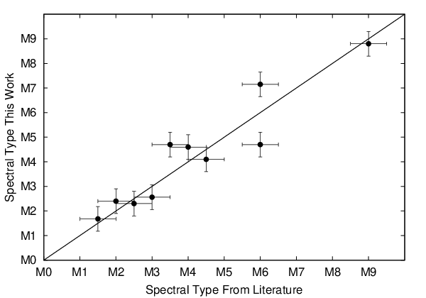

Appendix C C. Details of Cross-Correlation Against Theoretical Spectral Templates
As an alternative method to determine the stellar atmospheric parameters we compare our disentangled NIR spectra to model spectra from the BT-Settl grid [3] computed using the Asplund et al. [4] solar abundances. The models have temperatures between 2600 K and 4000 K in steps of 100 K, and have [Fe/H] metallicities between dex and dex in dex increments. A metallicity of [Fe/H] dex is also included. The models assume solar-scaled abundances with -enhancement for sub-solar metallicities such that [/Fe] for [Fe/H], and [/Fe] for [Fe/H]. We only considered templates with .
The model spectra are broadened to the resolution of our observations and then cross-correlated using the XCSAO routine, which is part of the RVSAO package [55]. We ignore rotational and turbulent broadening which are both much lower than the instrumental resolution (the expected projected rotation speeds are and for the primary and secondary stars, respectively). The correlation is performed separately for the , , , and -bands.
We first determine effective temperatures for each of the stars as follows. The normalized cross-correlation peak-height is recorded for each model in the grid, and we fit a paraboloid to values near the peak that is a function of [Fe/H] and Teff. The Teff value at the peak location is recorded for each band. We then determine best-estimates of the Teff, and uncertainties, for each star, still analyzing each bandpass separately, using a similar technique to what was done for the spectroscopic indices. We conducted an MCMC analysis to explore a likelihood function as in equation B1, with now being the effective temperature, and replacing with . Here is an additional free parameter and is the median S/N ratio for spectrum of star . This results in Teff measurements and uncertainties for each star, in each of the four bandpasses. We then combine the four separate bandpasses by using another MCMC and a similar likelihood function. In this case the index enumerates the different bands, and we use , as the uncertainty for band of star , rather than . We do this rather than simply taking the weighted average of the four bandpasses as we found that the scatter between bands exceeded the measurement uncertainties, and this is a straightforward method to account for the additional systematic error. The resulting effective temperatures have uncertainties of K.
Figure 19 compares the effective temperatures estimated in this manner to the spectral types estimated using the H2OK indices. In this plot we also show the relations from Bessell [10], Luhman et al. [59], and Rajpurohit et al. [71]. We find that our effective temperatures and spectral types are in good agreement with the Rajpurohit et al. [71] relation, in which effective temperatures are determined by cross-correlating optical spectra against BT-Settl synthetic templates.
Having determined the effective temperature for each star, we next determine the [Fe/H] metallicity. We do this in a similar manner to the effective temperatures, except we fix the temperature to the best-estimated value for each star when finding a [Fe/H] value that maximizes the correlation for a given spectrum and band. We exclude the -band which we found to yield [Fe/H] values that are systematically lower than the other three bands by dex. This band also generally has a lower cross-correlation peak-height than the other bands indicating systematic differences between the models and observations in this wavelength range. The resulting [Fe/H] values have uncertainties of dex66 6 If we do not fix the temperature in finding the [Fe/H] values, the results have much larger scatter ( to dex) and do not correlate with the metallicities based on the spectroscopic indices.. Figure 20 compares the [Fe/H] values so-determined to the values based on the Terrien et al. [88] - and -band indices. The two methods yield metallicities that, aside from one significant outlier in NLTT 15867, are fairly consistent. If we remove NLTT 15867, then the cross-correlation-based metallicities are dex lower than the T12 metallicities. A difference on this order is not surprising given the different assumed solar abundance patterns on which each metallicity system is based. Comparing to metallicities based on the Rojas-Ayala et al. [76] indices yields similar results.
For HAT-TR-318-007A and HAT-TR-318-007B we find effective temperatures of T K and T K, respectively, from cross-correlation, and metallicities of [Fe/H] and [Fe/H], respectively. Combining the metallicities of the primary and secondary components yields a metallicity for the system of [Fe/H], which is consistent with the system metallicity determined from the T12 indicators.


